Asymptotically optimal, sequential, multiple testing procedures with prior information on the number of signals

Abstract

Assuming that data are collected sequentially from independent streams, we consider the simultaneous testing of multiple binary hypotheses under two general setups; when the number of signals (correct alternatives) is known in advance, and when we only have a lower and an upper bound for it. In each of these setups, we propose feasible procedures that control, without any distributional assumptions, the familywise error probabilities of both type I and type II below given, user-specified levels. Then, in the case of i.i.d. observations in each stream, we show that the proposed procedures achieve the optimal expected sample size, under every possible signal configuration, asymptotically as the two error probabilities vanish at arbitrary rates. A simulation study is presented in a completely symmetric case and supports insights obtained from our asymptotic results, such as the fact that knowledge of the exact number of signals roughly halves the expected number of observations compared to the case of no prior information.

and

1 Introduction

Multiple testing, that is the simultaneous consideration of $K$ hypothesis testing problems, $H_{0}^{k}$ versus $H_{1}^{k}$, $1\leq k\leq K$, is one of the oldest, yet still very active areas of statistical research. The vast majority of work in this area assumes a fixed set of observations and focuses on testing procedures that control the familywise type I error (i.e., at least one false positive), as in Marcus, Eric and Gabriel (1976); Holm (1979); Hommel (1988), or less stringent metrics of this error, as in Benjamini and Hochberg (1995) and Lehmann and Romano (2005).

The multiple testing problem has been less studied under the assumption that observations are acquired sequentially, in which case the sample size is random. The sequential setup is relevant in many applications, such as multichannel signal detection (Mei, 2008; Dragalin, Tartakovsky and Veeravalli, 1999), outlier detection (Li, Nitinawarat and Veeravalli, 2014), clinical trials with multiple end-points (Bartroff and Lai, 2008), ultra high throughput mRNA sequencing data (Bartroff and Song, 2013), in which it is vital to make a quick decision in real time, using the smallest possible number of observations.

Bartroff and Lai (2010) were the first to propose a sequential test that controls the familywise error of type I. De and Baron (2012a, b) and Bartroff and Song (2014) proposed universal sequential procedures that control simultaneously the familywise errors of both type I and type II, a feature that is possible due to the sequential nature of sampling. The proposed sequential procedures in these works were shown through simulation studies to offer substantial savings in the average sample size in comparison to the corresponding fixed-sample size tests.

A very relevant problem to multiple testing is the classification problem, in which there are $M$ hypotheses, $H_{1},\ldots,H_{M}$, and the goal is to select the correct one among them. The classification problem has been studied extensively in the literature of sequential analysis, see e.g. Sobel and Wald (1949); Armitage (1950); Lorden (1977); Tartakovsky (1998); Dragalin, Tartakovsky and Veeravalli (1999, 2000), generalizing the seminal work of Wald (1945) on binary testing $(M=2)$. Dragalin, Tartakovsky and Veeravalli (2000) considered the multiple testing problem as a special case of the classification problem under the assumption of a single signal in $K$ independent streams, and focused on procedures that control the probability of erroneously claiming the signal to be in stream $i$ for every $1\leq i\leq M=K$. In this framework, they proposed an asymptotically optimal sequential test as all these error probabilities go to 0. The same approach of treating the multiple testing problem as a classification problem has been taken by Li, Nitinawarat and Veeravalli (2014) under the assumption of an upper bound on the number of signals in the $K$ independent streams, and a single control on the maximal mis-classification probability.

We should stress that interpreting multiple testing as a classification problem does not generally lead to feasible procedures. Consider, for example, the case of no prior information, which is the default assumption in the multiple testing literature. Then, multiple testing becomes a classification problem with $M=2^{K}$ categories and a brute-force implementation of existing classification procedures becomes infeasible even for moderate values of $K$, as the number of statistics that need to be computed sequentially grows exponentially with $K$. Independently of feasibility considerations, to the best of our knowledge there is no optimality theory regarding the expected sample size that can be achieved by multiple testing procedures, with or without prior information, that control the familywise errors of both type I and type II. Filling this gap was one of the motivations of this paper.

The main contributions of the current work are the following: first of all, assuming that the data streams that correspond to the various hypotheses are independent, we propose feasible procedures that control the familywise errors of both type I and type II below arbitrary, user-specified levels. We do so under two general setups regarding prior information; when the true number of signals is known in advance, and when there is only a lower and an upper bound for it. The former setup includes the case of a single signal considered in Dragalin, Tartakovsky and Veeravalli (1999, 2000), whereas the latter includes the case of no prior information, which is the underlying assumption in De and Baron (2012a, b); Bartroff and Song (2014). While we provide universal threshold values that guarantee the desired error control in the spirit of the above works, we also propose a Monte Carlo simulation method based on importance sampling for the efficient calculation of non-conservative thresholds in practice, even for very small error probabilities. More importantly, in the case of independent and identically distributed (i.i.d.) observations in each stream, we show that the proposed multiple testing procedures attain the optimal expected sample size, for any possible signal configuration, to a first-order asymptotic approximation as the two error probabilities go to zero in an arbitrary way. Our asymptotic results also provide insights about the effect of prior information on the number of signals, which are corroborated by a simulation study.

The remainder of the paper is organized as follows. In Section 2 we formulate the problem mathematically. In Section 3 we present the proposed procedures and show how they can be designed to guarantee the desired error control. In Section 4 we propose an efficient Monte Carlo simulation method for the determination of non-conservative critical values in practice. In Section 5 we establish the asymptotic optimality of the proposed procedures in the i.i.d. setup. In Section 6 we illustrate our asymptotic results with a simulation study. In Section 7 we conclude and discuss potential generalizations of our work. Finally, we present two useful lemmas for our proofs in an Appendix.

2 Problem formulation

Consider $K$ independent streams of observations, $X^{k}:=\{X_{n}^{k}:n\in\mathbb{N}\}$, $k\in[K]$, where $[K]:=\{1,\ldots,K\}$ and $\mathbb{N}:=\{1,2,\ldots\}$. For each $k\in[K]$, let ${\sf P}^{k}$ be the distribution of $X^{k}$, for which we consider two simple hypotheses,

$$H_{0}^{k}:\;{\sf P}^{k}={\sf P}_{0}^{k}\;\text{ versus }\;H_{1}^{k}:\;{\sf P}^{k}={\sf P}_{1}^{k},$$

where ${\sf P}_{0}^{k}$ and ${\sf P}_{1}^{k}$ are distinct probability measures on the canonical space of $X^{k}$. We will say that there is “noise” in the $k^{th}$ stream under ${\sf P}_{0}^{k}$ and “signal” under ${\sf P}_{1}^{k}$. Our goal is to simultaneously test these $K$ hypotheses when data from all streams become available sequentially and we want to make a decision as soon as possible.

Let $\mathcal{F}_{n}$ be the $\sigma$-field generated by all streams up to time $n$, i.e., $\mathcal{F}_{n}=\sigma(X_{1},\ldots,X_{n})$, where $X_{n}=(X_{n}^{1},\ldots,X_{n}^{K})$. We define a sequential test for the multiple testing problem of interest to be a pair $(T,d)$ that consists of an $\{\mathcal{F}_{n}\}$-stopping time, $T$, at which we stop sampling in all streams, and an $\mathcal{F}_{T}$-measurable decision rule, $d=(d^{1},\ldots,d^{K})$, each component of which takes values in $\{0,1\}$. The interpretation is that we declare upon stopping that there is signal (resp. noise) in the $k^{th}$ stream when $d^{k}=1$ (resp. $d^{k}=0$). With an abuse of notation, we will also use $d$ to denote the subset of streams in which we declare that signal is present, i.e., $\{k\in[K]:\;d^{k}=1\}$.

For any subset $\mathcal{A}\subset[K]$ we define the probability measure

$${\sf P}_{\mathcal{A}}:=\bigotimes_{k=1}^{K}{\sf P}^{k};\qquad\;{\sf P}^{k}=\begin{cases}{\sf P}_{0}^{k},\qquad\text{ if }k\notin\mathcal{A}\\ {\sf P}_{1}^{k},\qquad\text{ if }k\in\mathcal{A}\end{cases},$$

such that the distribution of $\{X_{n},n\in\mathbb{N}\}$ is ${\sf P}_{\mathcal{A}}$ when $\mathcal{A}$ is the true subset of signals, and for an arbitrary sequential test $(T,d)$ we set:

$$\{\mathcal{A}\lesssim d\} :=\{(d\setminus\mathcal{A})\neq\emptyset\}=\bigcup_{j\not\in\mathcal{A}}\{d^{j}=1\},$$

$$\{d\lesssim\mathcal{A}\} :=\{(\mathcal{A}\setminus d)\neq\emptyset\}=\bigcup_{k\in\mathcal{A}}\{d^{k}=0\}.$$

Then, ${\sf P}_{\mathcal{A}}(\mathcal{A}\lesssim d)$ is the probability of at least one false positive (familywise type I error) and ${\sf P}_{\mathcal{A}}\left(d\lesssim\mathcal{A}\right)$ the probability of at least one false negative (familywise type II error) of $(T,d)$ when the true subset of signals is $\mathcal{A}$.

In this work we are interested in sequential tests that control these probabilities below user-specified levels $\alpha$ and $\beta$ respectively, where $\alpha,\beta\in(0,1)$, for any possible subset of signals. In order to be able to incorporate prior information, we assume that the true subset of signals is known to belong to a class $\mathcal{P}$ of subsets of $[K]$, not necessarily equal to the powerset, and we focus on sequential tests in the class

$$\Delta_{\alpha,\beta}(\mathcal{P}):=\left\{(T,d):{\sf P}_{\mathcal{A}}(\mathcal{A}\lesssim d)\leq\alpha\;\;\text{and}\;\;{\sf P}_{\mathcal{A}}\left(d\lesssim\mathcal{A}\right)\leq\beta\;\;\text{for every}\;\;\mathcal{A}\in\mathcal{P}\right\}.$$

We consider, in particular, two general cases for class $\mathcal{P}$. In the first one, it is known that there are exactly $m$ signals in the $K$ streams, where $1\leq m\leq K-1$. In the second, it is known that there are at least $\ell$ and at most $u$ signals, where $0\leq\ell<u\leq K$. In the former case we write $\mathcal{P}=\mathcal{P}_{m}$ and in the latter $\mathcal{P}=\mathcal{P}_{\ell,u}$, where

$$\mathcal{P}_{m}:=\left\{\mathcal{A}\subset[K]:|\mathcal{A}|=m\right\},\quad\mathcal{P}_{\ell,u}:=\left\{\mathcal{A}\subset[K]:\ell\leq|\mathcal{A}|\leq u\right\}.$$

When $\ell=0$ and $u=K$, the class $\mathcal{P}_{\ell,u}$ is the powerset of $[K]$, which corresponds to the case of no prior information regarding the multiple testing problem.

Our main focus is on multiple testing procedures that not only belong to $\Delta_{\alpha,\beta}(\mathcal{P})$ for a given class $\mathcal{P}$, but also achieve the minimum possible expected sample size, under each possible signal configuration, for small error probabilities. To be more specific, let $\mathcal{P}$ be a given class of subsets and let $(T^{*},d^{*})$ be a sequential test that can designed to belong to $\Delta_{\alpha,\beta}(\mathcal{P})$ for any given $\alpha,\beta\in(0,1)$. We say that $(T^{*},d^{*})$ is asymptotically optimal with respect to class $\mathcal{P}$, if for every $\mathcal{A}\in\mathcal{P}$ we have as $\alpha,\beta\to 0$

$${\sf E}_{\mathcal{A}}\left[T^{*}\right]\sim\inf_{(T,d)\in\Delta_{\alpha,\beta}(\mathcal{P})}{\sf E}_{\mathcal{A}}\left[T\right],$$

where ${\sf E}_{\mathcal{A}}$ refers to expectation under ${\sf P}_{\mathcal{A}}$ and $x\sim y$ means that $x/y\rightarrow 1$. The ultimate goal of this work is to propose feasible sequential tests that are asymptotically optimal with respect to classes of the form $\mathcal{P}_{m}$ and $\mathcal{P}_{\ell,u}$.

2.1 Assumptions and notations

Before we continue with the presentation and analysis of the proposed multiple testing procedures, we will introduce some additional notation, and impose some minimal conditions on the distributions in each stream, which we will assume to hold throughout the paper.

First of all, for each stream $k\in[K]$ and time $n\in\mathbb{N}$ we assume that the probability measures ${\sf P}_{0}^{k}$ and ${\sf P}_{1}^{k}$ are mutually absolutely continuous when restricted to the $\sigma$-algebra $\mathcal{F}_{n}^{k}=\sigma(X_{1}^{k},\ldots,X_{n}^{k})$, and we denote by

$$\lambda^{k}(n):=\log\frac{d{\sf P}_{1}^{k}}{d{\sf P}_{0}^{k}}(\mathcal{F}_{n}^{k})$$ (1)

the cumulative log-likelihood ratio at time $n$ based on the data in the $k^{th}$ stream. Moreover, we assume that for each stream $k\in[K]$ the probability measures ${\sf P}_{0}^{k}$ and ${\sf P}_{1}^{k}$ are singular on $\mathcal{F}_{\infty}^{k}:=\sigma(\cup_{n\in\mathbb{N}}\mathcal{F}_{n}^{k})$, which implies that

$${\sf P}_{0}^{k}\left(\lim_{n\to\infty}\lambda^{k}(n)=-\infty\right)={\sf P}_{1}^{k}\left(\lim_{n\to\infty}\lambda^{k}(n)=\infty\right)=1.$$ (2)

Intuitively, this means that as observations accumulate, the evidence in favor of the correct hypothesis becomes arbitrarily strong. The latter assumption is necessary in order to design procedures that terminate almost surely under every scenario. We do not make any other distributional assumption until Section 5.

We use the following notation for the ordered, local, log-likelihood ratio statistics at time $n$:

$$\lambda^{(1)}(n)\geq\ldots\geq\lambda^{(K)}(n),$$

and we denote by $i_{1}(n),\ldots,i_{K}(n)$ the corresponding stream indices, i.e.,

$$\lambda^{(k)}(n)=\lambda^{i_{k}(n)}(n),\text{ for every }k\in[K].$$

Moreover, for every $n\in\mathbb{N}$ we denote by $p(n)$ the number of positive log-likelihood ratio statistics at time $n$, i.e.,

$$\lambda^{(1)}(n)\geq\ldots\geq\lambda^{(p(n))}(n)>0\geq\lambda^{(p(n)+1)}(n)\geq\ldots\geq\lambda^{(K)}(n).$$

For any two subsets $\mathcal{A},\mathcal{C}\subset[K]$ we denote by $\lambda^{\mathcal{A},\mathcal{C}}$ the log-likelihood ratio process of ${\sf P}_{\mathcal{A}}$ versus ${\sf P}_{\mathcal{C}}$, i.e.,

$$\lambda^{\mathcal{A},\mathcal{C}}(n) :=\log\frac{d{\sf P}_{\mathcal{A}}}{d{\sf P}_{\mathcal{C}}}(\mathcal{F}_{n})=\sum_{k\in\mathcal{A}\setminus\mathcal{C}}\lambda^{k}(n)-\sum_{k\in\mathcal{C}\setminus\mathcal{A}}\lambda^{k}(n),\quad n\in\mathbb{N}.$$ (3)

Finally, we use $|\cdot|$ to denote set cardinality, for any two real numbers $x,y$ we set $x\wedge y=\min\{x,y\}$ and $x\vee y=\max\{x,y\}$, and for any measurable event $\Gamma$ and random variable $Y$ we use the following notation

$${\sf E}_{\mathcal{A}}[Y;\Gamma]:=\int_{\Gamma}Yd{\sf P}_{\mathcal{A}}.$$

3 Proposed sequential multiple testing procedures

In this section we present the proposed procedures and show how they can be designed in order to guarantee the desired error control.

3.1 Known number of signals

In this subsection we consider the setup in which the number of signals is known to be equal to $m$ for some $1\leq m\leq K-1$, thus, $\mathcal{P}=\mathcal{P}_{m}$. Without loss of generality, we restrict ourselves to multiple testing procedures $(T,d)$ such that $|d|=m$. Thus, the class of admissible sequential tests takes the form

$$\Delta_{\alpha,\beta}(\mathcal{P}_{m})=\left\{(T,d):\;{\sf P}_{\mathcal{A}}(d\neq\mathcal{A})\leq\alpha\wedge\beta\,\;\text{for every}\;\mathcal{A}\in\mathcal{P}_{m}\right\},$$

since for any $\mathcal{A}\in\mathcal{P}_{m}$ and $(T,d)$ such that $|d|=m$ we have

$$\{\mathcal{A}\lesssim d\}\;=\;\{d\lesssim\mathcal{A}\}\;=\;\{d\neq\mathcal{A}\}.$$

In this context, we propose the following sequential scheme: stop as soon as the gap between the $m$-th and $(m+1)$-th ordered log-likelihood ratio statistics becomes larger than some constant $c>0$, and declare that signal is present in the $m$ streams with the top log-likelihood ratios at the time of stopping. Formally, we propose the following procedure, to which we refer as “gap rule”:

$$\begin{split}T_{G}&:=\inf\left\{n\geq 1:\lambda^{(m)}(n)-\lambda^{(m+1)}(n)\geq c\right\},\\ d_{G}&:=\{i_{1}(T_{G}),\ldots,i_{m}(T_{G})\}.\end{split}$$ (4)

Here, we suppress the dependence of $(T_{G},d_{G})$ on $m$ and $c$ to lighten the notation. The next theorem shows how to select threshold $c$ in order to guarantee the desired error control.

Theorem 3.1.

Suppose that assumption (2) holds. Then, for any $\mathcal{A}\in\mathcal{P}_{m}$ and $c>0$ we have ${\sf P}_{A}(T_{G}<\infty)=1$ and

$${\sf P}_{\mathcal{A}}\left(d_{G}\neq\mathcal{A}\right)\leq m(K-m)e^{-c}.$$ (5)

Consequently, $(T_{G},d_{G})\in\Delta_{\alpha,\beta}(\mathcal{P}_{m})$ when threshold $c$ is selected as

$$c=|\log(\alpha\wedge\beta)|+\log(m(K-m)).$$ (6)

Proof.

Fix $\mathcal{A}\in\mathcal{P}_{m}$ and $c>0$. We observe that $T_{G}\leq T_{G}^{\prime}$, where

$$\begin{split}T^{\prime}_{G}&=\inf\left\{n\geq 1:\lambda^{(m)}(n)-\lambda^{(m+1)}(n)\geq c,\;i_{1}(n)\in\mathcal{A},\ldots,i_{m}(n)\in\mathcal{A}\right\}\\ &=\inf\left\{n\geq 1:\lambda^{k}(n)-\lambda^{j}(n)\geq c\;\;\text{for every}\,k\in\mathcal{A}\;\text{and}\;j\notin\mathcal{A}\right\}.\end{split}$$ (7)

Due to condition (2), it is clear that ${\sf P}_{\mathcal{A}}(T_{G}^{\prime}<\infty)=1$, which proves that $T_{G}$ is also almost surely finite under ${\sf P}_{\mathcal{A}}$. We now focus on proving (5). The gap rule makes a mistake under ${\sf P}_{\mathcal{A}}$ if there exist $k\in\mathcal{A}$ and $j\notin\mathcal{A}$ such that the event $\Gamma_{k,j}=\left\{\lambda^{j}(T_{G})-\lambda^{k}(T_{G})\geq c\right\}$ occurs. In other words,

$$\left\{d_{G}\neq\mathcal{A}\right\}=\bigcup_{k\in\mathcal{A},j\notin\mathcal{A}}\Gamma_{k,j},$$

and from Boole’s inequality we have

$${\sf P}_{\mathcal{A}}(d_{G}\neq\mathcal{A})\leq\sum_{k\in\mathcal{A},j\notin\mathcal{A}}{\sf P}_{\mathcal{A}}(\Gamma_{k,j}).$$

Fix $k\in\mathcal{A},j\notin\mathcal{A}$ and set $\mathcal{C}=\mathcal{A}\cup\{j\}\setminus\{k\}$. Then, from (3) we have that $\lambda^{\mathcal{A},\mathcal{C}}=\lambda^{k}-\lambda^{j}$ and from Wald’s likelihood ratio identity it follows that

$$\begin{split}{\sf P}_{\mathcal{A}}(\Gamma_{k,j})&={\sf E}_{\mathcal{C}}\left[\exp\{\lambda^{\mathcal{A},\mathcal{C}}(T_{G})\};\Gamma_{k,j}\right]\\ &={\sf E}_{\mathcal{C}}\left[\exp\{\lambda^{k}(T_{G})-\lambda^{j}(T_{G})\};\Gamma_{k,j}\right]\leq e^{-c},\end{split}$$ (8)

where the last inequality holds because $\lambda^{j}(T_{G})-\lambda^{k}(T_{G})\geq c$ on $\Gamma_{k,j}$. Since $|\mathcal{A}|=m$ and $|\mathcal{A}^{c}|=K-m$, from the last two inequalities we obtain (5), which completes the proof. ∎

3.2 Lower and upper bounds on the number of signals

In this subsection, we consider the setup in which we know that there are at least $\ell$ and at most $u$ signals for some $0\leq\ell<u\leq K$, that is, $\mathcal{P}=\mathcal{P}_{\ell,u}$. In order to describe the proposed procedure, it is useful to first introduce the “intersection rule”, $(T_{I},d_{I})$, according to which we stop sampling as soon as all log-likelihood ratio statistics are outside the interval $(-a,b)$, and at this time we declare that signal is present (resp. absent) in those streams with positive (resp. negative) log-likelihood ratio, i.e.,

$$\begin{split}T_{I}&:=\inf\left\{n\geq 1:\lambda^{k}(n)\not\in(-a,b)\;\;\text{for every}\;k\in[K]\right\},\\ d_{I}&:=\{i_{1}(T_{I}),\ldots,i_{p(T_{I})}(T_{I})\},\end{split}$$ (9)

recalling that $p(n)$ is the number of positive log-likelihood ratios at time $n$. This procedure was proposed by De and Baron (2012a), where it was also shown that when the thresholds are selected as

$$a=|\log\beta|+\log K,\quad b=|\log\alpha|+\log K,$$ (10)

the familywise type-I and type-II error probabilities are bounded by $\alpha$ and $\beta$ for any possible signal configuration, i.e., $(T_{I},d_{I})\in\Delta_{\alpha,\beta}(\mathcal{P}_{0,K})$.

A straightforward way to incorporate the prior information of at least $\ell$ and at most $u$ signals in the intersection rule is to modify the stopping time in (9) as follows:

$$\tau_{2} :=\inf\left\{n\geq 1:\ell\leq p(n)\leq u\;\text{and}\;\lambda^{k}(n)\not\in(-a,b)\;\text{for every}\;k\in[K]\right\},$$ (11)

while keeping the same decision rule as in (9). Indeed, stopping according to $\tau_{2}$ guarantees that the number of null hypotheses rejected upon stopping will be between $\ell$ and $u$. However, as we will see in Subsection 5.3, this rule will not in general achieve asymptotic optimality in the boundary cases of exactly $\ell$ and exactly $u$ signals. In order to obtain an asymptotically optimal rule, we need to be able to stop faster when there are exactly $\ell$ or $u$ signals, which can be achieved by stopping at

$$\tau_{1} :=\inf\left\{n\geq 1:\lambda^{(\ell+1)}(n)\leq-a,\;\lambda^{(\ell)}(n)-\lambda^{(\ell+1)}(n)\geq c\right\},$$

$$\quad\text{and}\quad\tau_{3} :=\inf\left\{n\geq 1:\lambda^{(u)}(n)\geq b,\;\lambda^{(u)}(n)-\lambda^{(u+1)}(n)\geq d\right\},$$

respectively. Here, $c$ and $d$ are additional positive thresholds that will be selected, together with $a$ and $b$, in order to guarantee the desired error control.

We can think of $\tau_{1}$ as a combination of the intersection rule and the gap rule that corresponds to the case of exactly $\ell$ signals. Indeed, $\tau_{1}$ stops when $K-\ell$ log-likelihood ratio statistics are simultaneously below $-a$, but unlike the intersection rule it does not wait for the remaining $\ell$ statistics to be larger than $b$; instead, similarly to the gap-rule in (4) with $m=\ell$, it requires the gap between the top $\ell$ and the bottom $K-\ell$ statistics to be larger than $c$. In a similar way, $\tau_{3}$ is a combination of the intersection rule and the gap rule that corresponds to the case of exactly $u$ signals.

Based on the above discussion, when we know that there are at least $\ell$ and at most $u$ signals, we propose the following procedure, to which we refer as “gap-intersection” rule:

$$T_{GI} :=\min\{\tau_{1},\tau_{2},\tau_{3}\},\quad d_{GI}:=\{i_{1}(T_{GI}),\ldots,i_{p^{\prime}}(T_{GI})\},$$ (12)

where $p^{\prime}:=(p(T_{GI})\wedge\ell)\vee u$ is a truncated version of the number of positive log-likelihood ratios at $T_{GI}$, i.e., if $p^{\prime}=\ell$ when $p(T_{GI})\leq\ell$, $p^{\prime}=u$ when $p(T_{GI})\geq u$ and $p^{\prime}=p(T_{GI})$ otherwise. In other words, we stop sampling as soon as one of the stopping criterion in $\tau_{1}$, $\tau_{2}$ or $\tau_{3}$ is is satisfied, and we reject upon stopping the null hypotheses in the $p^{\prime}$ streams with the highest log-likelihood ratio values at time $T_{GI}$.

As before, we suppress the dependence on $\ell,u$ and $a,b,c,d$ in order to lighten the notation. Moreover, we set $\lambda^{(0)}(n)=-\infty$ and $\lambda^{(K+1)}(n)=\infty$ for every $n\in\mathbb{N}$, which implies that if $\ell=0$, then $\tau_{1}=\infty$, and if $u=K$, then $\tau_{3}=\infty$. When in particular $\ell=0$ and $u=K$, that is the case of no prior information, $T_{GI}=\tau_{2}$ and $(T_{GI},d_{GI})$ reduces to the intersection rule, $(T_{I},d_{I})$, defined in (9).

The following theorem shows how to select thresholds $a,b,c,d$ in order to guarantee the desired error control for the gap-intersection rule.

Theorem 3.2.

Suppose that assumption (2) holds. For any subset $\mathcal{A}\in\mathcal{P}_{\ell,u}$ and positive thresholds $a,b,c,d$, we have ${\sf P}_{A}(T_{GI}<\infty)=1$ and

$$\begin{split}{\sf P}_{\mathcal{A}}(\mathcal{A}\lesssim d_{GI})&\,\leq|\mathcal{A}^{c}|\,\left(e^{-b}+|\mathcal{A}|\,e^{-c}\right),\\ {\sf P}_{\mathcal{A}}(d_{GI}\lesssim\mathcal{A})&\,\leq|\mathcal{A}|\,\left(e^{-a}+|\mathcal{A}^{c}|\,e^{-d}\right).\end{split}$$ (13)

In particular, $(T_{GI},d_{GI})\in\Delta_{\alpha,\beta}(\mathcal{P}_{\ell,u})$ when the thresholds $a,b,c,d$ are selected as follows:

$$\begin{split}a&=|\log\beta|+\log K,\quad d=|\log\beta|+\log(uK),\\ b&=|\log\alpha|+\log K,\quad c=|\log\alpha|+\log((K-\ell)K).\end{split}$$ (14)

Proof.

Fix $\mathcal{A}\in\mathcal{P}_{\ell,u}$ and $a,b,c,d>0$. Observe that $T_{GI}\leq\tau_{2}\leq\tau_{2}^{\prime}$, where

$$\tau_{2}^{\prime}=\inf\{n\geq 1:-\lambda^{j}(n)\geq a,\;\lambda^{k}(n)\geq b\;\;\text{for every}\;k\in\mathcal{A},j\notin\mathcal{A}\}.$$ (15)

Due to assumption (2), ${\sf P}_{\mathcal{A}}(\tau_{2}^{\prime}<\infty)=1$, which proves that $T_{GI}$ is also almost surely finite under ${\sf P}_{\mathcal{A}}$. We now focus on proving the bound in (13) for the familywise type-II error probability, since the corresponding result for the familywise type-I error can be shown similarly. From Boole’s inequality we have

$${\sf P}_{\mathcal{A}}(d_{GI}\lesssim\mathcal{A})={\sf P}_{\mathcal{A}}\left(\bigcup_{k\in\mathcal{A}}\{d_{GI}^{k}=0\}\right)\leq\sum_{k\in\mathcal{A}}{\sf P}_{\mathcal{A}}\left(d_{GI}^{k}=0\right).$$ (16)

Fix $k\in\mathcal{A}$. Whenever the gap-intersection rule mistakenly accepts $H_{0}^{k}$, either the event $\Gamma_{k}:=\{\lambda^{k}(T_{GI})\leq-a\}$ occurs (which is the case when stopping at $\tau_{1}$ or $\tau_{2}$), or there is at least one $j\notin\mathcal{A}$ such that the event $\Gamma_{k,j}:=\{\lambda^{j}(T_{GI})-\lambda^{k}(T_{GI})\geq d\}$ occurs (which is the case when stopping at $\tau_{3}$). Therefore,

$$\{d_{GI}^{k}=0\}\subset\Gamma_{k}\cup(\cup_{j\notin\mathcal{A}}\Gamma_{k,j}),$$

and from Boole’s inequality we have

$${\sf P}_{\mathcal{A}}(d_{GI}^{k}=0)\leq{\sf P}_{\mathcal{A}}(\Gamma_{k})+\sum_{j\notin\mathcal{A}}{\sf P}_{\mathcal{A}}\left(\Gamma_{k,j}\right).$$

Identically to (8) we can show that for every $j\notin\mathcal{A}$ we have ${\sf P}_{\mathcal{A}}\left(\Gamma_{k,j}\right)\leq e^{-d}.$ Moreover, if we set $\mathcal{C}=A\setminus\{k\}$ (note that $C\notin\mathcal{P}_{\ell,u}$, but this does not affect our argument), then $\lambda^{\mathcal{A},\mathcal{C}}=\lambda^{k}$ and from Wald’s likelihood ratio identity we have

$${\sf P}_{\mathcal{A}}(\Gamma_{k}) ={\sf E}_{\mathcal{C}}\left[\exp\{\lambda^{\mathcal{A},\mathcal{C}}(T_{GI})\};\Gamma_{k}\right]={\sf E}_{\mathcal{C}}\left[\exp\{\lambda^{k}(T_{GI})\};\Gamma_{k}\right]\leq e^{-a}.$$

Thus,

$${\sf P}_{\mathcal{A}}(d^{k}_{GI}=0)\leq e^{-a}+(K-|\mathcal{A}|)e^{-d},$$

which together with (16) yields

$${\sf P}_{\mathcal{A}}(d_{GI}\lesssim\mathcal{A}) \,\leq|\mathcal{A}|(e^{-a}+|\mathcal{A}^{c}|e^{-d})\leq\frac{|\mathcal{A}|}{K}(Ke^{-a})+\frac{|\mathcal{A}^{c}|}{K}(uKe^{-d}).$$

Therefore, if the thresholds are selected according to (14), then $Ke^{-a}=\beta$ and $uKe^{-d}=\beta,$ which implies that

$${\sf P}_{\mathcal{A}}(d_{GI}\lesssim\mathcal{A})\leq\frac{|\mathcal{A}|}{K}\beta+\frac{|\mathcal{A}^{c}|}{K}\beta=\beta,$$

and the proof is complete. ∎

4 Computation of familywise error probabilities via importance sampling

The threshold specifications in (6) and (14) guarantee the desired error control for the gap rule and gap-intersection rule respectively, however they can be very conservative. In practice, it is preferable to use Monte Carlo simulation to determine the thresholds that equate (at least, approximately) the maximal familywise type I and type II error probabilities to the corresponding target levels $\alpha$ and $\beta$, respectively. Note that this needs to be done offline, before the implementation of the procedure.

When $\alpha$ and $\beta$ are very small, the corresponding errors are “rare events” and plain Monte Carlo will not be efficient. For this reason, in this section we propose a Monte Carlo approach based on importance sampling for the efficient computation of the familywise error probabilities of the proposed multiple testing procedures.

To be more specific, let $\mathcal{A}\subset[K]$ be the true subset of signals and consider the computation of the familywise type I error probability, ${\sf P}_{\mathcal{A}}(\mathcal{A}\lesssim d)$, of an arbitrary multiple testing procedure, $(T,d)$. The idea of importance sampling is to find a probability measure ${\sf P}_{\mathcal{A}}^{*}$, under which the stopping time $T$ is finite almost surely, and compute the desired probability by estimating (via plain Monte Carlo) the expectation in the right-hand side of the following identity:

$${\sf P}_{\mathcal{A}}(\mathcal{A}\lesssim d)={\sf E}^{*}_{\mathcal{A}}\left[(\Lambda^{*}_{\mathcal{A}})^{-1};\mathcal{A}\lesssim d\right],$$

which is obtained by an application of Wald’s likelihood ratio identity. Here, we denote by $\Lambda_{\mathcal{A}}^{*}$ the likelihood ratio of ${\sf P}^{*}_{\mathcal{A}}$ against ${\sf P}_{\mathcal{A}}$ at time $T$, i.e.,

$$\Lambda^{*}_{\mathcal{A}}=\frac{d{\sf P}^{*}_{\mathcal{A}}}{d{\sf P}_{\mathcal{A}}}(\mathcal{F}_{T}),$$

and by ${\sf E}^{*}_{\mathcal{A}}$ the expectation under ${\sf P}^{*}_{\mathcal{A}}$. The proposal distribution ${\sf P}^{*}_{\mathcal{A}}$ should be selected such that $\Lambda^{*}_{\mathcal{A}}$ is “large” on the event $\{\mathcal{A}\lesssim d\}$ and “small” on its complement. This intuition will guide us in the selection of ${\sf P}^{*}_{\mathcal{A}}$ for the proposed rules.

For the gap rule $(T_{G},d_{G})$ we suggest the proposal distribution to be a uniform mixture over $\{{\sf P}_{\mathcal{A}\cup\{j\}\setminus\{k\}},k\in\mathcal{A},j\notin\mathcal{A}\}$, i.e.,

$${\sf P}^{G}_{\mathcal{A}}:=\frac{1}{|\mathcal{A}|\,|\mathcal{A}^{c}|}\sum_{k\in\mathcal{A}}\sum_{j\notin\mathcal{A}}{\sf P}_{\mathcal{A}\cup\{j\}\setminus\{k\}},$$ (17)

whose likelihood ratio against ${\sf P}_{\mathcal{A}}$ at time $T_{G}$ is

$$\Lambda^{G}_{\mathcal{A}} :=\frac{1}{|\mathcal{A}|\,|\mathcal{A}^{c}|}\sum_{k\in\mathcal{A}}\sum_{j\notin\mathcal{A}}\exp\{\lambda^{j}(T_{G})-\lambda^{k}(T_{G})\}.$$

Then, on the event $\{\mathcal{A}\lesssim d_{G}\}$ there exists some $k\in\mathcal{A}$ and $j\notin\mathcal{A}$ such that $\lambda^{j}(T_{G})-\lambda^{k}(T_{G})\geq c$, which leads to a large value for $\Lambda^{G}_{\mathcal{A}}$. On the other hand, on the complement of $\{\mathcal{A}\lesssim d_{G}\}$, $\{d_{G}=\mathcal{A}\}$, we have $\lambda^{j}(T_{G})-\lambda^{k}(T_{G})\leq-c$ for every $k\in\mathcal{A},j\notin\mathcal{A}$, which leads to a value of $\Lambda^{G}_{\mathcal{A}}$ close to 0.

For the intersection rule $(T_{I},d_{I})$ we suggest the proposal distribution to be a uniform mixture over $\{{\sf P}_{\mathcal{A}\cup\{j\}},j\notin\mathcal{A}\}$, i.e.,

$${\sf P}_{\mathcal{A}}^{I}:=\frac{1}{|\mathcal{A}^{c}|}\sum_{j\notin\mathcal{A}}{\sf P}_{\mathcal{A}\cup\{j\}},$$ (18)

whose likelihood ratio against ${\sf P}_{\mathcal{A}}$ at time $T_{I}$ takes the form

$$\Lambda^{I}_{\mathcal{A}}:=\frac{1}{|\mathcal{A}^{c}|}\sum_{j\notin\mathcal{A}}\exp\{\lambda^{j}(T_{I})\}.$$

Note that on the event $\{\mathcal{A}\lesssim d_{I}\}$ there exists some $j\notin A$ such that $\lambda^{j}(T_{I})\geq b$, which results in a large value for $\Lambda^{I}_{\mathcal{A}}$. On the other hand, on the complement of $\{\mathcal{A}\lesssim d_{I}\}$ we have $\lambda^{j}(T_{I})\leq-a$ for every $j\notin\mathcal{A}$, which results in a value of $\Lambda^{I}_{\mathcal{A}}$ close to 0.

Finally, for the gap-intersection rule we suggest to use ${\sf P}_{\mathcal{A}}^{I}$, the same proposal distribution as in the intersection rule, when $\ell<|\mathcal{A}|<u$. In the boundary case, i.e. $|\mathcal{A}|=\ell$ or $|\mathcal{A}|=u$, we propose the following mixture of ${\sf P}_{\mathcal{A}}^{G}$ and ${\sf P}_{\mathcal{A}}^{I}$:

$${\sf P}^{GI}_{\mathcal{A}}:=\frac{|\mathcal{A}|}{1+|\mathcal{A}|}\,{\sf P}_{\mathcal{A}}^{G}+\frac{1}{1+|\mathcal{A}|}\,{\sf P}_{\mathcal{A}}^{I}.$$

In Section 6 we apply the proposed simulation approach for the specification of non-conservative thresholds in the case of identical, symmetric hypotheses with Gaussian i.i.d. data. We also refer to Song and Fellouris (2016) for an analysis of these importance sampling estimators.

5 Asymptotic optimality in the i.i.d. setup

From now on, we assume that, for each stream $k\in[K]$, the observations $\{X_{n}^{k},n\in\mathbb{N}\}$ are independent random variables with common density $f_{i}^{k}$ with respect to a $\sigma$-finite measure $\mu^{k}$ under ${\sf P}_{i}^{k}$, $i=0,1$, such that the Kullback––Leibler information numbers

$$D_{0}^{k}:=\int\log\left(\frac{f_{0}^{k}}{f_{1}^{k}}\right)f_{0}^{k}d\mu^{k},\quad D_{1}^{k}:=\int\log\left(\frac{f_{1}^{k}}{f_{0}^{k}}\right)f_{1}^{k}d\mu^{k}$$

are both positive and finite. As a result, for each $k\in[K]$ the log-likelihood ratio process in the $k^{th}$ stream, defined in (1), takes the form

$$\lambda^{k}(n)=\sum_{j=1}^{n}\log\frac{f_{1}^{k}(X_{j}^{k})}{f_{0}^{k}(X_{j}^{k})},\quad n\in\mathbb{N},$$

and it is a random walk with drift $D_{1}^{k}$ under ${\sf P}_{1}^{k}$ and $-D_{0}^{k}$ under ${\sf P}_{0}^{k}$.

Our goal in this section is to show that the proposed multiple testing procedures in Section 3 are asymptotically optimal. Our strategy for proving this is first to establish a non-asymptotic lower bound on the minimum possible expected sample size in $\Delta_{\alpha,\beta}(\mathcal{P})$ for some arbitrary class $\mathcal{P}$, and then show that this lower bound is attained by the gap rule when $\mathcal{P}=\mathcal{P}_{m}$ and by the gap-intersection rule when $\mathcal{P}=\mathcal{P}_{\ell,u}$ as $\alpha,\beta\rightarrow 0$.

5.1 A lower bound on the optimal performance

In order to state the lower bound on the optimal performance, we introduce the function

$$\varphi(x,y):=x\log\left(\frac{x}{1-y}\right)+(1-x)\log\left(\frac{1-x}{y}\right),\quad x,y\in(0,1),$$ (19)

and for any subsets $\mathcal{C},\mathcal{A}\subset[K]$ such that $\mathcal{C}\neq\mathcal{A}$ we set

$$\gamma_{\mathcal{A},\mathcal{C}}(\alpha,\beta):=\begin{cases}\varphi(\alpha,\beta),\quad&\text{ if }\mathcal{C}\setminus\mathcal{A}\neq\emptyset,\;\mathcal{A}\setminus\mathcal{C}=\emptyset,\\ \varphi(\beta,\alpha),&\text{ if }\mathcal{C}\setminus\mathcal{A}=\emptyset,\;\mathcal{A}\setminus\mathcal{C}\neq\emptyset,\\ \varphi(\alpha,\beta)\vee\varphi(\beta,\alpha),\quad&\text{ otherwise}.\end{cases}$$

Theorem 5.1.

For any class $\mathcal{P}$, $\mathcal{A}\in\mathcal{P}$ and $\alpha,\beta\in(0,1)$ such that $\alpha+\beta<1$ we have

$$\inf_{(T,d)\in\Delta_{\alpha,\beta}(\mathcal{P})}{\sf E}_{\mathcal{A}}[T]\geq\max_{\mathcal{C}\in\mathcal{P},\mathcal{C}\not=\mathcal{A}}\,\frac{\gamma_{\mathcal{A},\mathcal{C}}(\alpha,\beta)}{\sum_{k\in\mathcal{A}\setminus\mathcal{C}}D_{1}^{k}+\sum_{k\in\mathcal{C}\setminus\mathcal{A}}D_{0}^{k}}.$$ (20)

Proof.

Fix $(T,d)\in\Delta_{\alpha,\beta}(\mathcal{P})$ and $\mathcal{A}\in\mathcal{P}$. Without loss of generality, we assume that ${\sf E}_{\mathcal{A}}[T]<\infty$. For any $\mathcal{C}\in\mathcal{P}$ such that $\mathcal{C}\neq\mathcal{A}$, the log-likelihood ratio process $\lambda^{\mathcal{A},\mathcal{C}}$, defined in (3), is a random walk under ${\sf P}_{\mathcal{A}}$ with drift equal to

$${\sf E}_{\mathcal{A}}[\lambda^{\mathcal{A},\mathcal{C}}(1)]=\sum_{k\in\mathcal{A}\setminus\mathcal{C}}D_{1}^{k}+\sum_{k\in\mathcal{C}\setminus\mathcal{A}}D_{0}^{k},$$

since each $\lambda^{k}$ is a random walk with drift $D_{1}^{k}$ under ${\sf P}_{1}^{k}$ and $-D_{0}^{k}$ under ${\sf P}_{0}^{k}$. Thus, from Wald’s identity it follows that

$${\sf E}_{\mathcal{A}}[T]=\frac{{\sf E}_{\mathcal{A}}[\lambda^{\mathcal{A},\mathcal{C}}(T)]}{\sum_{k\in\mathcal{A}\setminus\mathcal{C}}D_{1}^{k}+\sum_{k\in\mathcal{C}\setminus\mathcal{A}}D_{0}^{k}},$$

and it suffices to show that for any $\mathcal{C}\in\mathcal{P}$ such that $\mathcal{C}\neq\mathcal{A}$ we have

$${\sf E}_{\mathcal{A}}[\lambda^{\mathcal{A},\mathcal{C}}(T)]\geq\gamma_{\mathcal{A},\mathcal{C}}(\alpha,\beta).$$ (21)

Suppose that $\mathcal{C}\setminus\mathcal{A}\neq\emptyset$ and let $j\in\mathcal{C}\setminus\mathcal{A}$. Then, from Lemma A.1 in the Appendix we have

$${\sf E}_{\mathcal{A}}\left[\lambda^{\mathcal{A},\mathcal{C}}(T)\right] ={\sf E}_{\mathcal{A}}\left[\log\frac{d{\sf P}_{\mathcal{A}}}{d{\sf P}_{\mathcal{C}}}(\mathcal{F}_{T})\right]\geq\varphi\left({\sf P}_{\mathcal{A}}(d^{j}=1),{\sf P}_{\mathcal{C}}(d^{j}=0)\right).$$

By the definition of $\Delta_{\alpha,\beta}(\mathcal{P})$, we have ${\sf P}_{\mathcal{A}}(d^{j}=1)\leq\alpha$ and ${\sf P}_{\mathcal{C}}(d^{j}=0)\leq\beta$. Since the function $\varphi(x,y)$ is decreasing on the set $\{(x,y):x+y\leq 1\}$, and by assumption $\alpha+\beta\leq 1$, we conclude that if $\mathcal{C}\setminus\mathcal{A}\neq\emptyset$, then

$${\sf E}_{\mathcal{A}}[\lambda^{\mathcal{A},\mathcal{C}}(T)]\geq\varphi(\alpha,\beta).$$

With a symmetric argument we can show that if $\mathcal{A}\setminus\mathcal{C}\neq\emptyset$, then

$${\sf E}_{\mathcal{A}}[\lambda^{\mathcal{A},\mathcal{C}}(T)]\geq\varphi(\beta,\alpha).$$

The two last inequalities imply (21), and this completes the proof. ∎

Remark 5.1.

By the definition of $\varphi$ in (19), we have

$$\varphi(\alpha,\beta)=|\log\beta|\,(1+o(1)),\quad\varphi(\beta,\alpha)=|\log\alpha\,|(1+o(1))$$ (22)

as $\alpha,\beta\to 0$ at arbitrary rates.

5.2 Asymptotic optimality of the proposed schemes

In what follows, we assume that for each stream $k\in[K]$ we have:

$$\int\left(\log\left(\frac{f_{0}^{k}}{f_{1}^{k}}\right)\right)^{2}f_{i}^{k}d\mu^{k}<\infty,\quad i=0,1.$$ (23)

Although this assumption is not necessary for the asymptotic optimality of the proposed rules to hold, it will allow us to use Lemma A.2 in the Appendix and obtain valuable insights regarding the effect of prior information on the optimal performance. Moreover, for each subset $\mathcal{A}\subset[K]$ we set:

$$\eta_{1}^{\mathcal{A}}:=\min_{k\in\mathcal{A}}D_{1}^{k},\qquad\eta_{0}^{\mathcal{A}}:=\min_{j\notin\mathcal{A}}D_{0}^{j},$$

and, following the convention that the minimum over the empty set is $\infty$, we define: $\eta_{1}^{\emptyset}=\eta_{0}^{[K]}:=\infty$.

5.2.1 Known number of signals

We will first show that the gap rule, defined in (4), is asymptotically optimal with respect to class $\mathcal{P}_{m}$, where $1\leq m\leq K-1$. In order to do so, we start with an upper bound on the expected sample size of this procedure.

Lemma 5.2.

Suppose that assumption  (23) holds. Then, for any $\mathcal{A}\in\mathcal{P}_{m}$, as $c\to\infty$ we have

$${\sf E}_{\mathcal{A}}[T_{G}]\leq\frac{c}{\eta_{1}^{\mathcal{A}}+\eta_{0}^{\mathcal{A}}}+O\left(m(K-m)\sqrt{c}\right).$$

Proof.

Fix $\mathcal{A}\in\mathcal{P}_{m}$. For any $c>0$ we have $T_{G}\leq T_{G}^{\prime}$, where $T_{G}^{\prime}$ is defined in (7), and it is the first time that all $m(K-m)$ processes of the form $\lambda^{k}-\lambda^{j}$ with $k\in\mathcal{A}\;\text{and}\;j\notin\mathcal{A}$ exceed $c$. Due to condition (23), each $\lambda^{k}-\lambda^{j}$ with $k\in\mathcal{A}\;\text{and}\;j\notin\mathcal{A}$ is a random walk under ${\sf P}_{\mathcal{A}}$ with positive drift $D_{1}^{k}+D_{0}^{j}$ and finite second moment. Therefore, from Lemma A.2 it follows that as $c\to\infty$:

$${\sf E}_{\mathcal{A}}[T_{G}^{\prime}]\leq c\left(\min_{k\in\mathcal{A},j\notin\mathcal{A}}(D_{1}^{k}+D_{0}^{j})\right)^{-1}+O\left(m(K-m)\sqrt{c}\right),$$

and this completes the proof, since $\min_{k\in\mathcal{A},j\notin\mathcal{A}}(D_{1}^{k}+D_{0}^{j})=\eta_{1}^{\mathcal{A}}+\eta_{0}^{\mathcal{A}}$. ∎

The next theorem establishes the asymptotic optimality of the gap rule.

Theorem 5.3.

Suppose assumption (23) holds and let the threshold $c$ in the gap rule be selected according to (6). Then for every $\mathcal{A}\in\mathcal{P}_{m}$, we have as $\alpha,\beta\to 0$

$${\sf E}_{\mathcal{A}}[T_{G}]\;\sim\;\frac{|\log(\alpha\wedge\beta)|}{\eta_{1}^{\mathcal{A}}+\eta_{0}^{\mathcal{A}}}\;\sim\;\inf_{(T,d)\in\Delta_{\alpha,\beta}(\mathcal{P}_{m})}{\sf E}_{\mathcal{A}}[T].$$

Proof.

Fix $\mathcal{A}\in\mathcal{P}_{m}$. If thresholds are selected according to  (6), then from Lemma 5.2 it follows that as $\alpha,\beta\to 0$

$${\sf E}_{\mathcal{A}}[T_{G}]\leq\frac{|\log(\alpha\wedge\beta)|}{\eta_{1}^{\mathcal{A}}+\eta_{0}^{\mathcal{A}}}+O\left(m(K-m)\sqrt{|\log(\alpha\wedge\beta)|}\right).$$ (24)

Therefore, it suffices to show that the lower bound in Theorem 5.1 agrees with the upper bound in (24) in the first-order term as $\alpha,\beta\to 0$. To see this, note that for any $\mathcal{C}\in\mathcal{P}_{m}$ such that $\mathcal{C}\neq\mathcal{A}$ we have $\mathcal{C}\setminus\mathcal{A}\neq\emptyset$ and $\mathcal{A}\setminus\mathcal{C}\neq\emptyset$, and consequently

$$\gamma_{\mathcal{A},\mathcal{C}}(\alpha,\beta)=\varphi(\alpha,\beta)\vee\varphi(\beta,\alpha).$$

This means that the numerator in (20) does not depend on $\mathcal{C}$. Moreover, if we restrict our attention to subsets in $\mathcal{P}_{m}$ that differ from $\mathcal{A}$ in two streams, i.e., subsets of the form $\mathcal{C}=\mathcal{A}\cup\{j\}\setminus\{k\}$ for some $k\in\mathcal{A}$ and $j\notin\mathcal{A}$, for which

$$\sum_{i\in\mathcal{A}\setminus\mathcal{C}}D_{1}^{i}+\sum_{i\in\mathcal{C}\setminus\mathcal{A}}D_{0}^{i}=D_{1}^{k}+D_{0}^{j},$$

then we have

$$\min_{\mathcal{C}\in\mathcal{P}_{m},\mathcal{C}\neq\mathcal{A}}\left[\sum_{i\in\mathcal{A}\setminus\mathcal{C}}D_{1}^{i}+\sum_{i\in\mathcal{C}\setminus\mathcal{A}}D_{0}^{i}\right] \leq\min_{k\in\mathcal{A},j\notin\mathcal{A}}\,\left[D_{1}^{k}+D_{0}^{j}\right]=\eta_{1}^{\mathcal{A}}+\eta_{0}^{\mathcal{A}}.$$

By the last inequality and Theorem 5.1 we obtain the following non-asymptotic lower bound, which holds for any $\alpha,\beta$ such that $\alpha+\beta<1$:

$$\inf_{(T,d)\in\Delta_{\alpha,\beta}(\mathcal{P}_{m})}{\sf E}_{\mathcal{A}}[T]\geq\frac{\max\{\varphi(\alpha,\beta),\varphi(\beta,\alpha)\}}{\eta_{1}^{\mathcal{A}}+\eta_{0}^{\mathcal{A}}}.$$

By (22), we have as $\alpha,\beta\rightarrow 0$

$$\max\{\varphi(\alpha,\beta),\varphi(\beta,\alpha)\}=|\log(\alpha\wedge\beta)|\,(1+o(1)).$$

Consequently,

$$\inf_{(T,d)\in\Delta_{\alpha,\beta}(\mathcal{P}_{m})}{\sf E}_{\mathcal{A}}\left(T\right)\geq\frac{|\log(\alpha\wedge\beta)|}{\eta_{1}^{\mathcal{A}}+\eta_{0}^{\mathcal{A}}}\,(1+o(1)),$$

which completes the proof. ∎

Remark 5.2.

It is interesting to consider the special case of identical hypotheses, in which $f_{1}^{k}=f_{1}$ and $f_{0}^{k}=f_{0}$, and consequently $D_{1}^{k}=D_{1}$ and $D_{0}^{k}=D_{0}$ for every $k\in[K]$. Then, $\eta_{1}^{\mathcal{A}}=D_{1}$ and $\eta_{0}^{\mathcal{A}}=D_{0}$ for every $\mathcal{A}\subset[K]$, and from Theorem 5.3 it follows that the first-order asymptotic approximation to the expected sample size of the gap rule (as well as to the optimal expected sample size within $\Delta_{\alpha,\beta}(\mathcal{P}_{m})$), $|\log(\alpha\wedge\beta)|/(D_{1}+D_{0})$, is independent of the number of signals, $m$. We should stress that this does not mean that the actual performance of the gap rule is independent of $m$. Indeed, the second term in the right-hand side of (24) suggests that the smaller $m(K-m)$ is, i.e., the further away the proportion of signals $m/K$ is from $1/2$, the smaller the expected sample size of the gap rule will be. This intuition will be corroborated by the simulation study in Section 6 (see Fig. 2).

5.2.2 Lower and upper bounds on the number of signals

We will now show that the gap-intersection rule, defined in (12), is asymptotically optimal with respect to class $\mathcal{P}_{\ell,u}$ for some $0\leq\ell<u\leq K$. As before, we start with establishing an upper bound on the expected sample size of this rule.

Lemma 5.4.

Suppose that assumption (23) holds. Then, for any $\mathcal{A}\in\mathcal{P}_{\ell,u}$ we have as $a,b,c,d\to\infty$

$${\sf E}_{\mathcal{A}}[T_{GI}]\leq\begin{cases}\max\left\{a/\eta_{0}^{\mathcal{A}}\;,\;c/(\eta_{0}^{\mathcal{A}}+\eta_{1}^{\mathcal{A}})\right\}(1+o(1))\;&\text{ if }\;|\mathcal{A}|=\ell\\ \max\left\{a/\eta_{0}^{\mathcal{A}}\;,\;b/\eta_{1}^{\mathcal{A}}\right\}+O(K\sqrt{a\vee b})\;&\text{ if }\;\ell<|\mathcal{A}|<u\\ \max\left\{b/\eta_{1}^{\mathcal{A}}\;,\;d/(\eta_{0}^{\mathcal{A}}+\eta_{1}^{\mathcal{A}})\right\}(1+o(1))\;&\text{ if }\;|\mathcal{A}|=u\end{cases}$$

Furthermore, if $c-a=O(1)$ and $d-b=O(1)$, then

$${\sf E}_{\mathcal{A}}[T_{GI}]\leq\begin{cases}a/\eta_{0}^{\mathcal{A}}+O((K-\ell)\sqrt{a})\quad&\text{ if }\;|\mathcal{A}|=\ell\\ b/\eta_{1}^{\mathcal{A}}+O(u\sqrt{b})\quad&\text{ if }\;|\mathcal{A}|=u\end{cases}$$ (25)

Proof.

Fix $\mathcal{A}\in\mathcal{P}_{\ell,u}$. By the definition of the stopping time $T_{GI}$,

$${\sf E}_{\mathcal{A}}[T_{GI}]\leq\min\left\{{\sf E}_{\mathcal{A}}[\tau_{1}],{\sf E}_{\mathcal{A}}[\tau_{2}],{\sf E}_{\mathcal{A}}[\tau_{3}]\right\}.$$

Suppose first $\ell<|\mathcal{A}|<u$ and observe that $\tau_{2}\leq\tau_{2}^{\prime}$, where $\tau_{2}^{\prime}$ is defined in (15). Under condition (23), for every $k\in\mathcal{A}$ and $j\notin\mathcal{A}$, $-\lambda^{j}$ and $\lambda^{k}$ are random walks with finite second moments and positive drifts $D_{0}^{j}$ and $D_{1}^{k}$, respectively. Therefore, from Lemma A.2 we have that

$${\sf E}_{\mathcal{A}}[\tau^{\prime}_{2}]\leq\max\left\{a/\eta_{0}^{\mathcal{A}}\;,\;b/\eta_{1}^{\mathcal{A}}\right\}+O(K\sqrt{a\vee b}).$$

Suppose now that $|\mathcal{A}|=\ell$ and observe that $\tau_{1}\leq\tau_{1}^{\prime}$, where

$$\tau_{1}^{\prime}:=\inf\{n\geq 1:-\lambda^{j}(n)\geq a,\;\lambda^{k}(n)-\lambda^{j}(n)\geq c\;\;\text{for every}\;k\in\mathcal{A},j\notin\mathcal{A}\},$$

where $-\lambda^{j}$ and $\lambda^{k}-\lambda^{j}$ are random walks with finite second moments and positive drifts $D_{0}^{j}$ and $D_{1}^{k}+D_{0}^{j}$, respectively. The result follows again from an application of Lemma A.2. If in addition we have that $c-a=O(1)$, then $\tau_{1}\leq\tau_{1}^{\prime\prime}$, where

$$\tau_{1}^{\prime\prime}:=\inf\{n\geq 1:-\lambda^{j}(n)\geq a,\;\lambda^{k}(n)\geq c-a\;\;\text{for every}\;k\in\mathcal{A},j\notin\mathcal{A}\}.$$

Therefore, the second part of the lemma follows again from an application of Lemma A.2. ∎

The next theorem establishes the asymptotic optimality of the gap-intersection rule.

Theorem 5.5.

Suppose that assumption (23) holds and let the thresholds in the gap-intersection rule be selected according to (14). Then for any $\mathcal{A}\in\mathcal{P}_{\ell,u}$, we have as $\alpha,\beta\to 0$

$${\sf E}_{\mathcal{A}}[T_{GI}]\; \sim\;\inf_{(T,d)\in\Delta_{\alpha,\beta}(\mathcal{P}_{\ell,u})}{\sf E}_{\mathcal{A}}[T]$$

$$\sim\;\begin{cases}\max\left\{|\log\beta|/\eta_{0}^{\mathcal{A}}\;,\;|\log\alpha|/(\eta_{0}^{\mathcal{A}}+\eta_{1}^{\mathcal{A}})\right\}\quad&\text{ if }\;|\mathcal{A}|=\ell\\ \max\left\{|\log\beta|/\eta_{0}^{\mathcal{A}}\;,\;|\log\alpha|/\eta_{1}^{\mathcal{A}}\right\}\quad&\text{ if }\;\ell<|\mathcal{A}|<u\\ \max\left\{|\log\alpha|/\eta_{1}^{\mathcal{A}}\;,\;|\log\beta|/(\eta_{0}^{\mathcal{A}}+\eta_{1}^{\mathcal{A}})\right\}\quad&\text{ if }\;|\mathcal{A}|=u\end{cases}.$$

Proof.

Fix $\mathcal{A}\in\mathcal{P}_{\ell,u}$. We will prove the result only in the case that $|\mathcal{A}|=\ell$, as the other two cases can be proved similarly. If thresholds are selected according to (14), then from Lemma 5.4 it follows that

$${\sf E}_{\mathcal{A}}[T_{GI}]\leq\max\left\{\frac{|\log\beta|}{\eta_{0}^{\mathcal{A}}}\;,\;\frac{|\log\alpha|}{\eta_{0}^{\mathcal{A}}+\eta_{1}^{\mathcal{A}}}\right\}\,(1+o(1)).$$

Thus, it suffices to show that this asymptotic upper bound agrees asymptotically, up to a first order, with the lower bound in Theorem 5.1. Indeed, if $\mathcal{C}$ is a subset in $\mathcal{P}_{\ell,u}$ that has one more stream than $\mathcal{A}$, i.e., $\mathcal{C}=\mathcal{A}\cup\{j\}$ for some $j\notin\mathcal{A}$, then

$$\frac{\gamma_{\mathcal{A},\mathcal{C}}(\alpha,\beta)}{\sum_{i\in\mathcal{A}\setminus\mathcal{C}}D_{1}^{i}+\sum_{i\in\mathcal{C}\setminus\mathcal{A}}D_{0}^{i}}=\frac{\varphi(\alpha,\beta)}{D_{0}^{j}}.$$

Further, consider $\mathcal{C}=\mathcal{A}\cup\{j\}/\{k\}\in\mathcal{P}_{\ell,u}$ for some $k\in\mathcal{A}$ and $j\notin\mathcal{A}$, then

$$\frac{\gamma_{\mathcal{A},\mathcal{C}}(\alpha,\beta)}{\sum_{i\in\mathcal{A}\setminus\mathcal{C}}D_{1}^{i}+\sum_{i\in\mathcal{C}\setminus\mathcal{A}}D_{0}^{i}}=\frac{\max\{\varphi(\alpha,\beta),\varphi(\beta,\alpha)\}}{D_{1}^{k}+D_{0}^{j}}.$$

Therefore, from (5.1) it follows that for every $\alpha,\beta$ such that $\alpha+\beta<1$

$$\inf_{(T,d)\in\Delta_{\alpha,\beta}(\mathcal{P}_{\ell,u})}{\sf E}_{\mathcal{A}}[T] \geq\max_{k\in\mathcal{A},j\notin\mathcal{A}}\max\left\{\frac{\varphi(\alpha,\beta)}{D_{0}^{j}}\;,\;\frac{\max\{\varphi(\alpha,\beta),\varphi(\beta,\alpha)\}}{D_{1}^{k}+D_{0}^{j}}\right\}$$

$$=\max\left\{\frac{\varphi(\alpha,\beta)}{\eta_{0}^{\mathcal{A}}},\;\frac{\varphi(\beta,\alpha)}{\eta_{1}^{\mathcal{A}}+\eta_{0}^{\mathcal{A}}}\right\}.$$

From (22) it follows that as $\alpha,\beta\to 0$

$$\inf_{(T,d)\in\Delta_{\alpha,\beta}(\mathcal{P}_{l,u})}{\sf E}_{\mathcal{A}}[T]\geq\max\left\{\frac{|\log\beta|}{\eta_{0}^{\mathcal{A}}},\;\frac{|\log\alpha|}{\eta_{1}^{\mathcal{A}}+\eta_{0}^{\mathcal{A}}}\right\}\,(1+o(1)),$$

which completes the proof. ∎

5.3 The case of no prior information

Recall that when we set $\ell=0$ and $u=K$, the gap-intersection rule reduces to the intersection rule, defined in (9). Therefore, setting $\ell=0$ and $u=K$ in Theorem 5.5 we immediately obtain that the intersection rule is asymptotically optimal in the case of no prior information, i.e., with respect to class $\mathcal{P}_{0,K}$; this is itself a new result to the best of our knowledge. However, a more surprising corollary of Theorem 5.5 is that the intersection rule, which does not use any prior information, is asymptotically optimal even if bounds on the number of signals are available, when the following conditions are satisfied:

1. the error probabilities are of the same order of magnitude, in the sense that $|\log\alpha|\sim|\log\beta|$,

2. the hypotheses are identical and symmetric, in the sense that $D_{1}^{k}=D_{0}^{k}=D$ for every $k\in[K]$.

On the other hand, a comparison with Theorem 5.3 reveals that, even in this special case, the intersection rule is never asymptotically optimal when the exact umber of signals is known in advance, in which case it requires roughly twice as many observations on average as the gap rule for the same precision level. The following corollary summarizes these observations.

Corollary 5.6.

Suppose that assumption (23) holds and that the thresholds in the intersection rule are selected according to (10). Then, for any $\mathcal{A}\subset[K]$ we have as $\alpha,\beta\rightarrow 0$

$${\sf E}_{\mathcal{A}}[T_{I}]\leq\max\left\{\frac{|\log\alpha|}{\eta_{1}^{\mathcal{A}}},\frac{|\log\beta|}{\eta_{0}^{\mathcal{A}}}\right\}+O(K\sqrt{|\log(\alpha\wedge\beta)|}).$$ (26)

Further, the intersection rule is asymptotically optimal in the class $\Delta_{\alpha,\beta}(\mathcal{P}_{0,K})$, i.e., as $\alpha,\beta\to 0$

$${\sf E}_{\mathcal{A}}[T_{I}]\;\sim\;\max\left\{\frac{|\log\alpha|}{\eta_{1}^{\mathcal{A}}},\frac{|\log\beta|}{\eta_{0}^{\mathcal{A}}}\right\}\;\sim\;\inf_{(T,d)\in\Delta_{\alpha,\beta}(\mathcal{P}_{0,K})}{\sf E}_{\mathcal{A}}[T].$$

In the special case that $|\log\alpha|\sim|\log\beta|$ and $D_{1}^{k}=D_{0}^{k}=D$ for every $k\in[K]$,

$${\sf E}_{\mathcal{A}}[T_{I}] \sim\;\frac{|\log\alpha|}{D}\;\sim\;\inf_{(T,d)\in\Delta_{\alpha,\beta}(\mathcal{P}_{\ell,u})}{\sf E}_{\mathcal{A}}[T]\quad\text{for every}\;\mathcal{A}\in\mathcal{P}_{\ell,u},$$

$${\sf E}_{\mathcal{A}}[T_{I}] \sim\;\frac{|\log\alpha|}{D}\;\sim\;2\,\inf_{(T,d)\in\Delta_{\alpha,\beta}(\mathcal{P}_{m})}{\sf E}_{\mathcal{A}}[T]\quad\text{for every}\;\mathcal{A}\in\mathcal{P}_{m},$$

for every $0\leq\ell<u\leq K$ and $1\leq m\leq K-1$.

Remark 5.3.

Corollary 5.6 implies that, in the special symmetric case that $|\log\alpha|\sim|\log\beta|$ and $D_{1}^{k}=D_{0}^{k}=D$, prior lower and upper bounds on the true number of signals do not improve the optimal expected sample size up to a first-order asymptotic approximation. However, a comparison between the second-order terms in (25) and (26) suggests that such prior information does improve the optimal performance, an intuition that will be corroborated by the simulation study in Section 6 (see Fig. 2).

Remark 5.4.

In addition to the intersection rule, De and Baron (2012a) proposed the “incomplete rule”, $(T_{\max},d_{\max})$, which is defined as

$$T_{\max}:=\max\{\sigma_{1},\ldots,\sigma_{K}\}\;\text{ and }\;d_{\max}:=(d_{\max}^{1},\ldots,d_{\max}^{K}),$$

where for every $k\in[K]$ we have

$$\sigma_{k} :=\inf\left\{n\geq 1:\lambda^{k}(n)\not\in(-a,b)\right\},\quad d_{\max}^{k}:=\begin{cases}1,\quad\text{ if }\lambda^{k}(\sigma_{k})\geq b\\ 0,\quad\text{ if }\lambda^{k}(\sigma_{k})\leq-a\end{cases}.$$ (27)

According to this rule, each stream is sampled until the corresponding test statistic exits the interval $(-a,b)$, independently of the other streams. It is clear that, for the same thresholds $a$ and $b$, $T_{\max}\leq T_{I}$. Moreover, with a direct application of Boole’s inequality, as in De and Baron (2012a), it follows that selecting the thresholds according to (10) guarantees the desired error control for the incomplete rule. Therefore, Corollary 5.6 remains valid if we replace the intersection rule with the incomplete rule.

6 Simulation study

6.1 Description

In this section we present a simulation study whose goal is to corroborate the asymptotic results and insights of Section 5 in the symmetric case described in Corollary 5.6. Thus, we set $K=10$ and let $f_{i}^{k}=\mathcal{N}(\theta_{i},1)$ for each $k\in[K]$, $i=0,1$, where $\theta_{0}=0,\theta_{1}=0.5$, in which case $D_{0}^{k}=D_{1}^{k}=D=(1/2)(\theta_{1})^{2}=1/8$, and the distribution of $\lambda^{k}$ under $H_{1}^{k}$ is the same as $-\lambda^{k}$ under $H_{0}^{k}$. Furthermore, we set $\alpha=\beta$. This is a convenient setup for simulation purposes, since the expected sample size and the two familywise errors of each proposed procedure are the same for all scenarios with the same number of signals, i.e. for all $\mathcal{A}$’s with the same size.

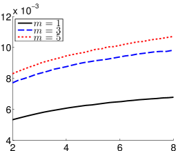
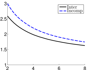
For any user specified level $\alpha$, we have two ways to determine the critical value of each procedure. First, we can use upper bound on the error probability to compute conservative threshold ((6) for the gap rule, and (14) for the gap-intersection rule). Second, we can apply the importance sampling technique of Section 4 to determine non-conservative threshold, such that the maximal familywise type I error probability is controlled exactly at level $\alpha$. As we see in Fig. 1, the relative errors of the proposed Monte Carlo estimators, even for error probabilities of the order $10^{-8}$, are smaller than $1.5\%$ for the gap rule, $8\%$ for the gap-intersection rule, $1\%$ for the intersection rule.

(a) Gap rule

(b) Gap-intersection rule

(c) Intersection rule

Figure 1: The x-axis is $|\log_{10}({\sf P}_{\mathcal{A}}(\mathcal{A}\lesssim d))|$. The y-axis is the relative error of the estimate of the familywise type-I error, ${\sf P}_{\mathcal{A}}(\mathcal{A}\lesssim d)$, that is the ratio of the standard deviation of the estimate over the estimate itself. Each curve is computed based on $100,000$ realizations.

6.1.1 Gap rule

First, we consider the case in which the number of signals is known to be equal to $m$ $(\mathcal{P}=\mathcal{P}_{m})$ for $m\in\{1,\ldots,9\}$, and we can apply the corresponding gap rule, defined in (4). Due to the symmetry of our setup, the expected sample size ${\sf E}_{\mathcal{A}}[T_{G}]$ and the error probability ${\sf P}_{\mathcal{A}}(d_{G}\neq\mathcal{A})$ are the same for $\mathcal{A}\in\mathcal{P}_{m}$ and $\mathcal{A}\in\mathcal{P}_{K-m}$; thus, it suffices to consider $m$ in $\{1,\ldots,5\}$ , and an arbitrary $\mathcal{A}\in\mathcal{P}_{m}$ for fixed $m$.

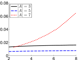
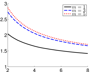
We start with non-conservative critical value determined by Monte Carlo method. For each $m\in\{1,3,5\}$ and some $\mathcal{A}\in\mathcal{P}_{m}$, we consider $\alpha$’s ranging from $10^{-2}$ to $10^{-8}$. For each such $\alpha$, we compute the threshold $c$ in the gap-rule that guarantees $\alpha={\sf P}_{\mathcal{A}}(d_{G}\neq\mathcal{A})$, and then the expected sample size ${\sf E}_{\mathcal{A}}[T_{G}]$ that corresponds to this threshold. In Fig. 2a we plot ${\sf E}_{\mathcal{A}}[T_{G}]$ against $|\log_{10}(\alpha)|$ when $m=1,3,5$. In Table 1a we present the actual numerical results for $c=10$.

In Fig. 2a we also plot the first-order asymptotic approximation to the optimal expected sample size obtained in Theorem 5.3, which in this particular symmetric case takes the form $|\log\alpha|/(2D)=4|\log\alpha|$. From our asymptotic theory we know that the ratio of ${\sf E}_{\mathcal{A}}[T_{G}]$ over this quantity goes to 1 as $\alpha\rightarrow 0$, and this convergence is illustrated in Fig. 2b.

Further, in Fig. 3a we present for the case $\mathcal{P}=\mathcal{P}_{3}$ the expected sample size of the gap rule when its threshold is given by the explicit expression in (6), and compare it with the corresponding expected sample size that is obtained with the sharp threshold, which is computed via simulation.

6.1.2 Gap-intersection rule

Second, we consider the case in which the number of signals is known to be between 3 and 7 ($\mathcal{P}=\mathcal{P}_{\ell,u}=\mathcal{P}_{3,7}$), and we can apply the gap-intersection rule, defined in (12). Due to the symmetry of the setup and Lemma 3.2, we set $a=b$ and $c=d=b+\log(u)=b+\log(7)$.

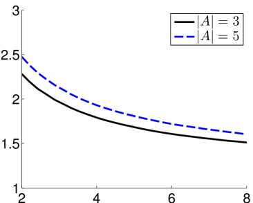
As before, we consider $\alpha$’s ranging from $10^{-2}$ to $10^{-8}$. For each such $\alpha$, we obtain the threshold $b$ such that $\max_{\mathcal{A}}{\sf P}_{\mathcal{A}}(\mathcal{A}\lesssim d_{GI})=\alpha$, where the maximum is taken over $\mathcal{A}\in\mathcal{P}_{\ell,u}$, and then compute the corresponding expected sample size ${\sf E}_{\mathcal{A}}[T_{GI}]$ for every $\mathcal{A}\in\mathcal{P}_{\ell,u}$. In Fig. 2c we plot ${\sf E}_{\mathcal{A}}[T_{GI}]$ against $|\log_{10}(\alpha)|$ for $|\mathcal{A}|=3$ and $5$, since by symmetry ${\sf E}_{\mathcal{A}}[T_{GI}]$ is the same for $|\mathcal{A}|=k$ and $10-k$, and the results for $|\mathcal{A}|=4$ and $5$ were too close. This is also evident from Table 1b, where we present the numerical results for $b=10$. In the same graph we also plot the first-order asymptotic approximation to the optimal performance obtained in Theorem 5.5, which in this case is $|\log\alpha|/D=8|\log\alpha|$. By Theorem 5.5, we know that the ratio of ${\sf E}_{\mathcal{A}}[T_{GI}]$ over $8|\log\alpha|$ goes to 1 as $\alpha\rightarrow 0$, which is corroborated in Fig. 2d.

6.1.3 Intersection versus incomplete rule

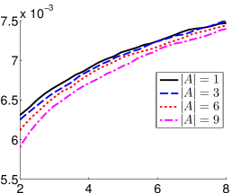
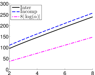
Finally, we consider the case of no prior information ($\mathcal{P}=\mathcal{P}_{0,10}$), in which we compare the intersection rule with the incomplete rule. This is a special case of the previous setup with $\ell=0$ and $u=K$, but now the expected sample size (for both schemes) is the same for every subset of signals $\mathcal{A}$, which allows us to plot only one curve for each scheme in Fig. 2e (non-conservative critical value is used). In the same graph we also plot the first-order approximation to the optimal performance, $|\log\alpha|/D=8|\log\alpha|$, whereas in Fig. 2f. we plot the corresponding normalized version.

Further, in Fig. 3b we present the expected sample size of the intersection rule when its threshold is given by the explicit expression in  (14), and compare it with the corresponding expected sample size that is obtained with the sharp threshold, which is computed via simulation.

6.2 Results

There are a number of conclusions that can be drawn from the presented graphs. First of all, from Fig. 2a it follows that the gap rule performs the best when there are exactly $m=1$ or $9$ signals, whereas its performance is quite similar for $m=3,4,5$. As we mentioned before, this can be explained by the fact that the second term in the right-hand side in (24) grows with $m(K-m)$.

Second, from Fig. 2c we can see that the gap-intersection rule performs better in the boundary cases that there are exactly 3 or 7 signals than in the case of 5 signals, which can be explained by the second order term in (25).

Third, from Fig. 2e we can see that the intersection rule is always better than the incomplete rule, although they share the same prior information.

Fourth, from the graphs in the second column of Fig. 2 we can see that all curves approach 1, as expected from our asymptotic results; however, the convergence is relatively slow. This is reasonable, as we do not divide the expected sample sizes by the optimal performance in each case, but with a strict lower bound on it instead.

Fifth, comparing Fig. 2a with Fig. 2c and 2e, we verify that knowledge of the exact number of signals roughly halves the required expected sample size in comparison to the case that we only have a lower and an upper bound on the number of signals.

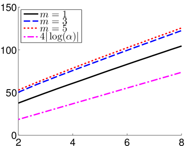
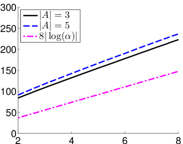
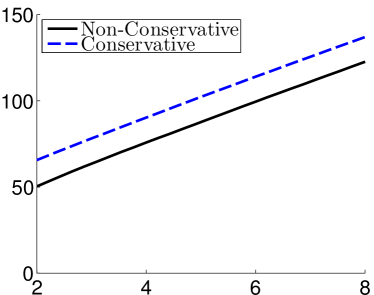
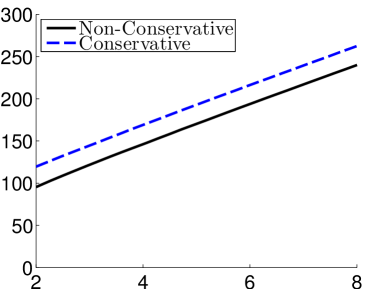
Finally, we see by Tables 1a and 1b that the upper bounds (5) and (13) on the error probabilities are very crude. Nevertheless, from Fig. 3a and 3b, we observe that using these conservative thresholds in the design of the proposed procedures leads to bounded performance loss as the error probabilities go to 0 relative to the case of sharp thresholds, obtained via Monte Carlo simulation. This is expected, as the expected sample size scales with the logarithm of the error probabilities.

(a) Gap rule: $\mathcal{P}=\mathcal{P}_{m}$, $m=1,3,5$

(b) Normalized by $4|\log(\alpha)|$

(c) Gap-intersection rule: $\mathcal{P}=\mathcal{P}_{3,7}$

(d) Normalized by $8|\log(\alpha)|$

(e) Intersection vs Incomplete: $\mathcal{P}=\mathcal{P}_{0,10}$

(f) Normalized by $8|\log(\alpha)|$

Figure 2: The x-axis in all graphs is $|\log_{10}(\alpha)|$. In the first column, the y-axis denotes the expected sample size under ${\sf P}_{\mathcal{A}}$ that is required in order to control the maximal familywise type I error probability exactly at level $\alpha$. The dash-dot lines in each plot correspond to the first-order approximation, which is also a lower bound, to the optimal expected sample size for the class $\Delta_{\alpha,\alpha}(\mathcal{P})$; due to symmetry, this lower bound does not depend on $|\mathcal{A}|$ in each setup. In the second column, we normalize each curve by its corresponding lower bound.

Table 1: The standard error of the estimate is included in the parenthesis. The upper bound is on the error control given by (5) for the first table and by (13) for the second.

$m$	${\sf P}_{\mathcal{A}}(d_{G}\neq\mathcal{A})$	${\sf E}_{\mathcal{A}}(T_{G})$	Upper bound
1	5.041E-05 (3.101E-07)	64.071 (0.157)	4.086E-4
3	6.034E-05 (5.343E-07)	78.386 (0.157)	9.534E-4
5	6.145E-05 (5.859E-07)	81.070 (0.156)	1.135E-3

(a) $\mathcal{P}=\mathcal{P}_{m}$. $(T_{G},d_{G})$ with $c=10$.

$|A|$	${\sf P}_{\mathcal{A}}(\mathcal{A}\lesssim d_{GI})$	${\sf E}_{\mathcal{A}}(T_{GI})$	Upper bound
3	3.653E-05 (5.447E-07)	142.173 (0.264)	4.540E-04
4	3.144E-05 (2.189E-07)	152.873 (0.264)	4.281E-04
5	2.621E-05 (1.825E-07)	152.895 (0.263)	3.891E-04
7	3.104E-07 (1.340E-08)	142.363 (0.270)	2.724E-04

(b) $\mathcal{P}=\mathcal{P}_{3,7}$. $(T_{GI},d_{GI})$ with $b=10$.

(a) Gap rule: $\mathcal{P}=\mathcal{P}_{3}$

(b) Intersection rule: $\mathcal{P}=\mathcal{P}_{0,10}$

Figure 3: The x-axis is $|\log_{10}(\alpha)|$, where $\alpha$ is user-specified level. The y-axis is the expected sample size. The dashed line uses the upper bound on the error probability to get conservative critical value, while the solid line uses the Monte Carlo approach to determine non-conservative threshold such that the maximal familywise type I error is controlled exactly at level $\alpha$.

7 Conclusions

We considered the problem of simultaneously testing multiple simple null hypotheses, each of them against a simple alternative, in a sequential setup. That is, the data for each testing problem are acquired sequentially and the goal is to stop sampling as soon as possible, simultaneously in all streams, and make a correct decision for each individual testing problem. The main goal of this work was to propose feasible, yet asymptotically optimal, procedures that incorporate prior information on the number of signals (correct alternatives), and also to understand the potential gains in efficiency by such prior information.

We studied this problem under the assumption that the data streams for the various hypotheses are independent. Without any distributional assumptions on the data that are acquired in each stream, we proposed procedures that control the probabilities of at least one false positive and at least one false negative below arbitrary user-specified levels. This was achieved in two general cases regarding the available prior information: when the exact number of signals is known in advance, and when we only have an upper and a lower bound for it. Furthermore, we proposed a Monte Carlo simulation method, based on importance sampling, that can facilitate the specification of non-conservative critical values for the proposed multiple testing procedures in practice. More importantly, in the special case of i.i.d. data in each stream, we were able to show that the proposed multiple testing procedures are asymptotically optimal, in the sense that they require the minimum possible expected sample size to a first-order asymptotic approximation as the error probabilities vanish at arbitrary rates.

These asymptotic optimality results have some interesting ramifications. First of all, they imply that any refinements of the proposed procedures, for example using a more judicious choice of alpha-spending and beta-spending functions, cannot reduce the expected sample size to a first-order asymptotic approximation. Second, they imply that bounds on the number of signals do not improve the minimum possible expected sample size to a first-order asymptotic approximation, apart from a very special case. On the other hand, knowledge of the exact number of signals does reduce the minimum possible expected sample size to a first order approximation, roughly by a factor of 2. These insights were corroborated by a simulation study, which however also revealed the limitations of a first-order asymptotic analysis and emphasized the importance of second-order terms.

To our knowledge, these are the first results on the asymptotic optimality of multiple testing procedures, with or without prior information, that control the familywise error probabilities of both types. However, there are still some important open questions that remain to be addressed. Do the proposed procedures attain, in the i.i.d. setup, the optimal expected sample size to a second-order asymptotic approximation as well? Does the first-order asymptotic optimality property remain valid for more general, non-i.i.d. data in the streams? While we conjecture that the answer to both these questions is affirmative, we believe that the corresponding proofs require different techniques from the ones we have used in the current paper.

There are also interesting generalizations of the setup we considered in this paper. For example, it is interesting to consider the sequential multiple testing problem when the goal is to control generalized error rates, such as the false discovery rate (Bartroff and Song, 2013), instead of the more stringent familywise error rates. Another interesting direction is to allow the hypotheses in the streams to be specified up to an unknown parameter, or to consider a non-parametric setup similarly to Li, Nitinawarat and Veeravalli (2014). Finally, it is still an open problem to design asymptotically optimal multiple testing procedures that incorporate prior information on the number of signals when it is possible and desirable to stop sampling at different times in the various streams.

Appendix A Two lemmas

A.1 An information-theoretic inequality

In the proof of Theorem 5.1 we use the following, well-known, information-theoretic inequality, whose proof can be found, e.g., in Tartakovsky, Nikiforov and Basseville (2014) (Chapter 3.2).

Lemma A.1.

Let ${\sf Q},{\sf P}$ be equivalent probability measures on a measurable space $(\Omega,\mathcal{G})$ and recall the function $\varphi$ defined in (19). Then, for every $A\in\mathcal{G}$ we have

$${\sf E}_{{\sf Q}}\left[\log\frac{d{\sf Q}}{d{\sf P}}\right]\geq\varphi\left(Q(A),{\sf P}(A^{c})\right).$$

A.2 A lemma on multiple random walks

For the proof of Lemmas 5.2 and 5.4 we need an upper bound on the expectation of the first time that multiple random walks, not necessarily independent, are simultaneously above given thresholds. We state here the corresponding result in some generality.

Thus, let $L\geq 2$ and suppose that for each $l\in[L]$ we have a sequence of i.i.d. random variables, $\{\xi_{n}^{l},n\in\mathbb{N}\}$, such that $\mu_{l}={\sf E}[\xi_{1}^{l}]>0$ and $\text{Var}[\xi_{1}^{l}]<\infty$. For each $l\in[L]$, let

$$S_{n}^{l}=\sum_{i=1}^{n}\xi_{i}^{l},\quad n\in\mathbb{N}$$

be the corresponding random walk. Here, no assumption is made on the dependence structure among these random walks. For an arbitrary vector $(a_{1},\ldots,a_{L})$, consider the stopping time

$$T=\inf\left\{n\geq 1\;:\;S_{n}^{l}\geq a_{l}\text{ for every }l\in[L]\right\}.$$

The following lemma provides an upper bound on the expected value of $T$. The proof is identical to the one in Theorem 2 in Mei (2008); thus we omit it. We stress that although the theorem in the reference assumes independent random walks, exactly the same proof applies to the case of dependent random walks.

Lemma A.2.

As $a_{1},\ldots,a_{L}\to\infty$,

$${\sf E}[T]\leq\max_{l\in[L]}\left(\frac{a_{l}}{\mu_{l}}\right)+O\left(\sum_{l\in[L]}\sqrt{\frac{a_{l}}{\mu_{l}}}\right)\leq\max_{l\in[L]}\left(\frac{a_{l}}{\mu_{l}}\right)+O\left(L\sqrt{\max_{l\in[L]}\{a_{l}\}}\right).$$

References

- Armitage (1950) {barticle}[author] \bauthor\bsnmArmitage, \bfnmP.\binitsP. (\byear1950). \btitleSequential Analysis with More than Two Alternative Hypotheses, and its Relation to Discriminant Function Analysis. \bjournalJournal of the Royal Statistical Society. Series B (Methodological) \bvolume12 \bpages137-144. \endbibitem
- Bartroff and Lai (2008) {barticle}[author] \bauthor\bsnmBartroff, \bfnmJay\binitsJ. and \bauthor\bsnmLai, \bfnmTze Leung\binitsT. L. (\byear2008). \btitleGeneralized likelihood ratio statistics and uncertainty adjustments in efficient adaptive design of clinical trials. \bjournalSequential Analysis \bvolume27 \bpages254–276. \endbibitem
- Bartroff and Lai (2010) {barticle}[author] \bauthor\bsnmBartroff, \bfnmJay\binitsJ. and \bauthor\bsnmLai, \bfnmTze Leung\binitsT. L. (\byear2010). \btitleMultistage tests of multiple hypotheses. \bjournalCommunications in Statistics–Theory and Methods \bvolume39 \bpages1597–1607. \endbibitem
- Bartroff and Song (2013) {barticle}[author] \bauthor\bsnmBartroff, \bfnmJ.\binitsJ. and \bauthor\bsnmSong, \bfnmJ.\binitsJ. (\byear2013). \btitleSequential Tests of Multiple Hypotheses Controlling False Discovery and Nondiscovery Rates. \bjournalarXiv:1311.3350 [stat.ME]. \endbibitem
- Bartroff and Song (2014) {barticle}[author] \bauthor\bsnmBartroff, \bfnmJay\binitsJ. and \bauthor\bsnmSong, \bfnmJinlin\binitsJ. (\byear2014). \btitleSequential tests of multiple hypotheses controlling type I and II familywise error rates. \bjournalJournal of statistical planning and inference \bvolume153 \bpages100–114. \endbibitem
- Benjamini and Hochberg (1995) {barticle}[author] \bauthor\bsnmBenjamini, \bfnmYoav\binitsY. and \bauthor\bsnmHochberg, \bfnmYosef\binitsY. (\byear1995). \btitleControlling the false discovery rate: a practical and powerful approach to multiple testing. \bjournalJournal of the Royal Statistical Society. Series B (Methodological) \bpages289–300. \endbibitem
- De and Baron (2012a) {barticle}[author] \bauthor\bsnmDe, \bfnmShyamal K\binitsS. K. and \bauthor\bsnmBaron, \bfnmMichael\binitsM. (\byear2012a). \btitleSequential Bonferroni methods for multiple hypothesis testing with strong control of family-wise error rates I and II. \bjournalSequential Analysis \bvolume31 \bpages238–262. \endbibitem
- De and Baron (2012b) {barticle}[author] \bauthor\bsnmDe, \bfnmShyamal K\binitsS. K. and \bauthor\bsnmBaron, \bfnmMichael\binitsM. (\byear2012b). \btitleStep-up and step-down methods for testing multiple hypotheses in sequential experiments. \bjournalJournal of Statistical Planning and Inference \bvolume142 \bpages2059–2070. \endbibitem
- Dragalin, Tartakovsky and Veeravalli (1999) {barticle}[author] \bauthor\bsnmDragalin, \bfnmVladimir P\binitsV. P., \bauthor\bsnmTartakovsky, \bfnmAlexander G\binitsA. G. and \bauthor\bsnmVeeravalli, \bfnmVenugopal V\binitsV. V. (\byear1999). \btitleMultihypothesis sequential probability ratio tests. I. Asymptotic optimality. \bjournalInformation Theory, IEEE Transactions on \bvolume45 \bpages2448–2461. \endbibitem
- Dragalin, Tartakovsky and Veeravalli (2000) {barticle}[author] \bauthor\bsnmDragalin, \bfnmVladimir P\binitsV. P., \bauthor\bsnmTartakovsky, \bfnmAlexander G\binitsA. G. and \bauthor\bsnmVeeravalli, \bfnmVenugopal V\binitsV. V. (\byear2000). \btitleMultihypothesis sequential probability ratio tests. II. Accurate asymptotic expansions for the expected sample size. \bjournalInformation Theory, IEEE Transactions on \bvolume46 \bpages1366–1383. \endbibitem
- Holm (1979) {barticle}[author] \bauthor\bsnmHolm, \bfnmSture\binitsS. (\byear1979). \btitleA simple sequentially rejective multiple test procedure. \bjournalScandinavian journal of statistics \bpages65–70. \endbibitem
- Hommel (1988) {barticle}[author] \bauthor\bsnmHommel, \bfnmGerhard\binitsG. (\byear1988). \btitleA stagewise rejective multiple test procedure based on a modified Bonferroni test. \bjournalBiometrika \bvolume75 \bpages383–386. \endbibitem
- Lehmann and Romano (2005) {barticle}[author] \bauthor\bsnmLehmann, \bfnmE. L.\binitsE. L. and \bauthor\bsnmRomano, \bfnmJoseph P.\binitsJ. P. (\byear2005). \btitleGeneralizations of the familywise error rate. \bjournalAnn. Statist. \bvolume33 \bpages1138–1154. \bdoi10.1214/009053605000000084 \endbibitem
- Li, Nitinawarat and Veeravalli (2014) {binproceedings}[author] \bauthor\bsnmLi, \bfnmYun\binitsY., \bauthor\bsnmNitinawarat, \bfnmSirin\binitsS. and \bauthor\bsnmVeeravalli, \bfnmVenugopal V\binitsV. V. (\byear2014). \btitleUniversal sequential outlier hypothesis testing. In \bbooktitleInformation Theory (ISIT), 2014 IEEE International Symposium on \bpages3205–3209. \bpublisherIEEE. \endbibitem
- Lorden (1977) {barticle}[author] \bauthor\bsnmLorden, \bfnmGary\binitsG. (\byear1977). \btitleNearly-optimal sequential tests for finitely many parameter values. \bjournalAnn. Statist. \bpages1–21. \endbibitem
- Marcus, Eric and Gabriel (1976) {barticle}[author] \bauthor\bsnmMarcus, \bfnmRuth\binitsR., \bauthor\bsnmEric, \bfnmPeritz\binitsP. and \bauthor\bsnmGabriel, \bfnmK Ruben\binitsK. R. (\byear1976). \btitleOn closed testing procedures with special reference to ordered analysis of variance. \bjournalBiometrika \bvolume63 \bpages655–660. \endbibitem
- Mei (2008) {barticle}[author] \bauthor\bsnmMei, \bfnmYajun\binitsY. (\byear2008). \btitleAsymptotic optimality theory for decentralized sequential hypothesis testing in sensor networks. \bjournalInformation Theory, IEEE Transactions on \bvolume54 \bpages2072–2089. \endbibitem
- Sobel and Wald (1949) {barticle}[author] \bauthor\bsnmSobel, \bfnmMilton\binitsM. and \bauthor\bsnmWald, \bfnmAbraham\binitsA. (\byear1949). \btitleA Sequential Decision Procedure for Choosing One of Three Hypotheses Concerning the Unknown Mean of a Normal Distribution. \bjournalAnn. Math. Statist. \bvolume20 \bpages502–522. \bdoi10.1214/aoms/1177729944 \endbibitem
- Song and Fellouris (2016) {binproceedings}[author] \bauthor\bsnmSong, \bfnmY.\binitsY. and \bauthor\bsnmFellouris, \bfnmG.\binitsG. (\byear2016). \btitleLogarithmically efficient simulation for misclassification probabilities in sequential multiple testing. In \bbooktitleProceedings of the Winter Simulation Conference. \bnote(accepted). \endbibitem
- Tartakovsky (1998) {barticle}[author] \bauthor\bsnmTartakovsky, \bfnmAlexander G\binitsA. G. (\byear1998). \btitleAsymptotic Optimality of Certain Multihypothesis Sequential Tests: Non-iid Case. \bjournalStatistical Inference for Stochastic Processes \bvolume1 \bpages265–295. \endbibitem
- Tartakovsky, Nikiforov and Basseville (2014) {bbook}[author] \bauthor\bsnmTartakovsky, \bfnmAlexander\binitsA., \bauthor\bsnmNikiforov, \bfnmIgor\binitsI. and \bauthor\bsnmBasseville, \bfnmMichèle\binitsM. (\byear2014). \btitleSequential analysis: Hypothesis testing and changepoint detection. \bpublisherCRC Press. \endbibitem
- Wald (1945) {barticle}[author] \bauthor\bsnmWald, \bfnmAbraham\binitsA. (\byear1945). \btitleSequential tests of statistical hypotheses. \bjournalThe Annals of Mathematical Statistics \bvolume16 \bpages117–186. \endbibitem