APCTP Pre2016-007
DESY 16-043
UT-16-12
Structure of Kähler potential
for
-term inflationary attractor models
Kazunori Nakayama(a,b), Ken’ichi Saikawa(c,d),
Takahiro Terada(a,e),
and Masahide Yamaguchi(d)
| a | Department of Physics, Faculty of Science, |
|---|---|
| The University of Tokyo, Bunkyo-ku, Tokyo 133-0033, Japan | |
| b | Kavli IPMU (WPI), UTIAS, |
| The University of Tokyo, Kashiwa, Chiba 277-8583, Japan | |
| c | Deutsches Elektronen-Synchrotron DESY, |
| Notkestrasse 85, 22607 Hamburg, Germany | |
| d | Department of Physics, Tokyo Institute of Technology, |
| Ookayama, Meguro-ku, Tokyo 152-8551, Japan | |
| e | Asia Pacific Center for Theoretical Physics (APCTP), |
| 67 Cheongam-ro, Nam-gu, Pohang 37673, South Korea |
Minimal chaotic models of -term inflation predicts too large primordial tensor perturbations. Although it can be made consistent with observations utilizing higher order terms in the Kähler potential, expansion is not controlled in the absence of symmetries. We comprehensively study the conditions of Kähler potential for -term plateau-type potentials and discuss its symmetry. They include the -attractor model with a massive vector supermultiplet and its generalization leading to pole inflation of arbitrary order. We extend the models so that it can describe Coulomb phase, gauge anomaly is cancelled, and fields other than inflaton are stabilized during inflation. We also point out a generic issue for large-field -term inflation that the masses of the non-inflaton fields tend to exceed the Planck scale.
1 Introduction
Inflation in the early universe is not only indispensable to explain horizon and longevity problems (see recent review, e.g. [1]) but also is strongly supported by the observations of cosmic microwave background anisotropies [2, 3, 4, 5]. The position of the first peak of the temperature-temperature correlations suggests spatially flat Universe as predicted by inflation, and the large scale anti-correlations in the temperature-E mode correlations implies the superhorizon epoch of primordial curvature perturbations, which can be naturally realized by inflation. Unfortunately, primordial tensor perturbations have not yet been found, which strongly constrains inflation model building. Actually, the recent results of the PLANCK collaboration place constraint on the tensor-to-scalar ratio as (95% CL, Planck TT+lowP) at , and when combined with BICEP2/Keck-Array, (95% CL, Planck TT+lowP+BKP) at the same pivot scale [4, 5]. This almost ruled out chaotic inflation models with quadratic and higher power-law potential. Instead, cosmological attractor models [6, 7, 8, 9, 10, 11, 12, 13] including conformal attractor model [14] and its extension to -attractor models [15, 16, 17, 18] have recently been getting more attention because they can easily fit the observed spectral index of the primordial curvature perturbations and accommodate observable tensor-to-scalar ratio rather arbitrarily. In Ref. [12], it became manifest that pole structure of order 2 in a kinetic term is important to realize this kind of -attractor models. This idea is further extended to pole inflation#1#1#1This terminology should not be confused with the pole-law inflation [19] proposed decades ago. [12, 20, 21], in which, around a pole of arbitrary order in the kinetic term, the potential becomes effectively flat after canonical normalization of the kinetic term.
On the other hand, in order to realize inflation including the above attractor models, supersymmetry (SUSY) is desired, which can control radiative corrections to the inflaton field to preserve the flatness of its potential. However, if one introduces local SUSY or supergravity,#2#2#2 For recent reviews of inflation in supergravity, see Refs. [22, 23, 24] we encounter difficulties again as corrections of order of the Hubble scale to the inflaton mass in -term inflation models [25]. This is because positive vacuum energy during inflation breaks SUSY and its effect as a SUSY breaking mass is in general transmitted to scalar fields including the inflaton. One way to circumvent this difficulty is to introduce a symmetry such as a shift symmetry [26, *Kawasaki:2000ws] to protect the flatness of the potential if one does not wish to adopt ad-hoc Kähler potential [28]. Another interesting possibility is to consider -term inflation [29, 30], which is free from the above problem thanks to the absence of the Hubble scale correction. The original -term inflation was proposed as hybrid inflation and later was extended to chaotic inflation [31, 32, 33]. However, as the observations are getting more and more precise, the predictions of simple models of -term inflation tend to conflict with the observational data unfortunately. Of course, as explicitly given in Sec. 2, if we take higher order terms of Kähler potential into account, such -term inflation models can still fit the observational data. But, such higher order terms are uncontrollable without symmetry. Then, instead, we revisit the attractor models in the context of -term inflation, which were discussed in the context of a massive vector supermultiplet [16, 34] and a Dirac-Born-Infeld action [35]. In this paper, we derive general conditions of Kähler potential necessary to realize -term inflationary attractor models in the context of pole inflation. Along the way, we point out a generic issue in large-field -term inflation to stabilize additional matter fields without knowledge of quantum gravity.
The paper is organized as follows. In the next section, we briefly review -term inflation models in supergravity and discuss the conflict of their predictions of simple models with the current data. As a simple extension, we take into account higher order corrections in Kähler potential and show how well such corrections improve the fit to the data. In Sec. 3, we revisit the -attractor models for -term inflation and extend the theory to the symmetric phase of gauge symmetry as well. We give a concrete workable example, in which the theory is well-defined almost everywhere on the field space and fields required for anomaly cancellation are stabilized during inflation. We also elucidate symmetries guaranteeing the (approximate) flatness of the -term potential. In Sec. 4, we generalize these results and derive a generic condition for Kähler potential to realize -term inflationary attractor models in the context of pole inflation. Final section is devoted to conclusion and discussions.
2 Large field -term inflation
In this section we briefly review large field -term inflation models and their problems. Hereafter, we take the reduced Planck unit unless otherwise stated. For the Kähler potential , the superpotential and the gauge kinetic function , the supergravity Lagrangian for the scalar field in the Einstein frame is
| (2.1) |
The scalar potential consists of -term and -term potential,
| (2.2) | |||
| (2.3) | |||
| (2.4) |
where is the inverse matrix of the Kähler metric , is the Kähler covariant derivative, and is the Killing vector of the Kähler manifold, which is in the case of linearly transforming fields under the U(1) symmetry with being the U(1) charge of . In this case, the -term potential reduces to the usual form,
| (2.5) |
Here, we do not consider the possibility of field-independent Fayet-Iliopoulos (FI) term or gauged U(1) -symmetry for simplicity.
2.1 -term inflation with monomial/polynomial potential
For simplicity, we consider a setup with two superfields and charged under U(1) gauge symmetry with charge and , respectively. Note that this is a minimal setup to avoid the gauge anomaly. Later we regard as an inflaton.#3#3#3All the following discussions do not change if we regard , instead of , as an inflaton. We also introduce a gauge-singlet superfield to stabilize fields other than the inflaton.#4#4#4Note that it may be possible that there is a non-trivial inflationary trajectory in a field space spanned by and without introducing any other stabilization term. For example, inflation can happen while and are rolling down toward the -flat direction. In this paper, we want to restrict ourselves to the case of exact single-field inflation as a first step to the model building, in which either or is responsible for inflation and other fields are heavy enough to be integrated out. In the case of -term models with stabilizer superfield whose -term component breaks SUSY during inflation, we can introduce a higher dimensional term like where is a field we want to stabilize during inflation. This generates a SUSY breaking mass term for . In our case of -term SUSY breaking during inflation, it is difficult to emulate this mechanism because the superfield acquiring -term is the gauge (vector) superfield, whose interaction is completely determined by the gauge symmetry. After all, this kind of coupling is just a part of -term potential. Therefore, we introduce a superpotential to stabilize additional fields. We assume the superpotential of the form
| (2.6) |
This can be viewed as a -dependent mass term for and . Then, for and , the -term potential is exactly flat for any . Hereafter we consider this configuration. Stability against and directions will be discussed in Sec. 2.2. We also take , with being a gauge coupling constant, in the following.
First of all, let us consider the minimal Kähler potential:
| (2.7) |
The kinetic term is canonical and the -term potential for is given by [33]
| (2.8) |
Therefore, we obtain a simple quartic inflaton potential and inflation occurs for .#5#5#5The angular component of is a Goldstone mode and does not affect the inflaton dynamics. This is a simple realization of model for chaotic inflation, but it contradicts with observations [5] since it predicts too large tensor-to-scalar ratio with being the -folding number after the observable scale exits the horizon. Typically we have depending on the thermal history after inflation.
One may extend the minimal model to include higher order terms in the Kähler potential:
| (2.9) |
We take to make () canonically normalized in the small field limit . The -term potential for with is given by
| (2.10) |
To be concrete, we assume the hierarchy and neglect terms with . Then the kinetic term is given by
| (2.11) |
and the -term potential is given by
| (2.12) |
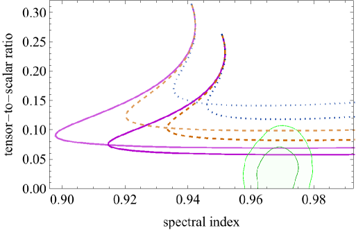
As shown in Refs. [36, 37, *Nakayama:2013txa], this kind of modification of the inflaton potential from the monomial to polynomial significantly changes the prediction of and we can make the fit to the observation better. In contrast to Refs. [36, 37, *Nakayama:2013txa], both the kinetic term (2.11) and potential (2.12) are determined solely by the Kähler potential and hence the structure of the potential in the canonical basis is more complicated. We assume in the following to improve the fit to observation. Note that we need the following condition if we require that for all ,
| (2.13) |
We can calculate the spectral index and tensor-to-scalar ratio by using the method given in Appendix A. The result is shown in Fig. 1. By choosing the parameter, we can make the prediction consistent with the Planck observation [5]. The overall magnitude of the density perturbation is reproduced for , hence this U(1) group cannot be identified with the subgroup of the standard model gauge group.
Another model is given in Appendix B, in which Kähler potential is expanded in terms of logarithm of inflaton field rather than the inflaton field itself. Due to this change, expansion of the canonical inflaton potential starts with lower powers than the quartic. Similarly to the above example, it is possible for its prediction to lie within the Planck contour by utilizing higher order terms in the Kähler potential.
Although it is possible to construct a model consistent with observations as above, it has several drawbacks. First, the Kähler potential is not controlled by any symmetry, hence there is no reason to expect that higher-order terms do not make comparable contributions to the results, which poses some doubts about the predictability of the model. Second, our calculation so far is based on an assumption that and are stabilized at . However, this assumption is not always justified, as we will see below.
2.2 Stabilization of other fields
Because of the structure of the -term potential (2.5), the oppositely charged field has a tachyonic mass during inflation,
| (2.14) |
where the subscript () represents the fact that these masses are obtained from -term (-term) potential, and denotes the Hubble parameter. In order to avoid such a tachyonic instability, we need to introduce the -term potential, which gives positive masses squared for and . With the superpotential (2.6), kinetic terms and -term potential for and during inflation are given by
| (2.15) | |||
| (2.16) |
where we have assumed that Kähler metric is diagonal around . This scalar potential to stabilize and is actually so steep that their masses easily exceed the Planck scale due to the large exponential factor . If we demand that their masses are larger than the Hubble scale at the end of inflation, their masses at the -folding is exponentially larger than the Hubble scale during inflation, which is typically much larger than the Planck scale. It means that quantum gravity effects may become important for inflationary region and the validity of the calculation is lost. This may be a general feature of large field -term inflation models in which fields other than the inflaton is strongly stabilized during inflation.#6#6#6Note that all the mass scales in the -term potential, including minimal SUSY standard model sector and SUSY breaking sector, are exponentially enhanced during inflation. While it is possible that there are no mass scales during inflation except for the -term potential in the inflaton sector, we stress that it might be non-trivial to have successful reheating and realistic SUSY model in such a setup.
This problem may be avoided by extending the structure of the Kähler potential for and . For example, let us take the following Kähler potential:
| (2.17) |
where is a constant. The addition of the last two terms does not affect the inflaton potential at . Then the physical -term masses of and in the canonical basis are
| (2.18) |
Note that and are almost identical during inflation since we can replace the factor in Eq. (2.3) with for . Therefore large exponential dependence is cancelled out with this kind of ad-hoc assumption on the Kähler potential and hence we can avoid the problem of too large masses for these fields. On the other hand, -term masses for and are given by
| (2.19) |
Therefore, we need , which implies , in order to stabilize at the origin during inflation.
3 Revisiting -term -attractor model
3.1 -term -attractor demystified and its symmetry
The -term -attractor model [16] had been constructed before the (-term) superconformal -attractor was discovered [17], but subsequent discussions of inflationary attractor models were mainly on -term models. Later, attractor models were understood as theories with second order pole in the kinetic term [12], which was further extended to arbitrary order poles [12, 20, 21]. So, let us tentatively pretend as if we do not know about the original -term attractor model, and consider its possibility in the perspective of general attractor or pole inflation context.
As repeatedly mentioned, the essence of the -attractor or more generally pole inflation is the presence of a pole in the kinetic term of the inflaton field before canonical normalization. With this in mind, a naive gauge-invariant choice for a possible -term attractor-type model would be
| (3.1) |
where is the inflaton field charged under U(1) symmetry, for simplicity, and other possible charged fields are neglected at this stage. This Kähler manifold has a curvature
| (3.2) | ||||
| (3.3) |
and leads to a second order pole in the kinetic term at ,
| (3.4) |
This apparently perfectly matches the requirement of pole inflation, and indeed this Kähler potential is used for -term -attractor models [17], though the appearance of the pole in the factor of scalar potential is cancelled out by the suitable choice of superpotential. There is another kind of difficulty in -term cases because not only the kinetic term but also the -term potential is determined by Kähler potential. When the Kähler metric has a second order pole, the -term potential, which contains , also has a second order pole generically. For the above Kähler potential, the scalar potential is
| (3.5) |
where is the canonical inflaton field. Thus, after canonical normalization, we obtain an exponentially steep function. Although a suitable choice of gauge kinetic function might in general rescue this situation like superpotential in -term cases, it is unlikely in our minimal setup because SUSY and gauge invariance require , and this reduces to a constant in our configuration . Exponential stretching due to canonical normalization is still valid, but the value of the potential grows rapidly near the pole, so the exponential flattening is not realized. This is because of the presence of the second order pole in the original scalar potential [21].
The -attractor model in the -term case was first discussed as an example of massive vector (or tensor) supermultiplet models [16]. In this approach, a U(1) vector supermultiplet and a chiral supermultiplet corresponding to a Higgs/Nambu-Goldstone field are introduced. Instead of taking Wess-Zumino gauge, gauge is chosen so that the chiral multiplet becomes trivial leading to the theory of a massive vector multiplet. This is just a SUSY description of the Higgs mechanism.
Here, we take Wess-Zumino gauge as usual, and retain a chiral superfield. Then, the -term model corresponding to the -attractor potential is given by [16]#7#7#7 Equation (4.31) of Ref. [16] contains a typo: either the term inside the logarithm or the second term should be multiplied by minus one. ,
| (3.6) |
where , . transforms nonlinearly like axion under the U(1) transformation, i.e. where is the transformation parameter, and the Killing vector is now given by with some constant . The field may be related to the usual U(1) charged field as , and is interpreted as the U(1) charge of . Inflation occurs in the large-field region of , and the imaginary part is absorbed by the gauge field due to the Higgs mechanism. It should be noted that the inflaton is not the shift symmetric direction in this case in contrast to the standard lore [26, *Kawasaki:2000ws, 39, 40]#8#8#8 It is possible to rewrite Eq. (3.6) in such a way that shift symmetry of the superfield corresponds to the shift symmetry of the canonical inflaton up to Kähler transformation, (3.7) In this expression, each of the first two terms is not gauge invariant, but it is when added up. . Note that the shift symmetry of in Eq. (3.6) becomes U(1) symmetry of in the Kähler potential
| (3.8) |
This kind of change of variables was discussed in the context of -term inflation [41]. In this parametrization of the field space, is defined only in . Inflation happens at large , and the phase component is absorbed by the Higgs mechanism. According to the general discussion of pole inflation [12, 20], which includes -attractor, potential can be flattened by a pole of the coefficient of kinetic term. To compare it with this notion, it may be useful to redefine the field ,
| (3.9) |
In this parametrization, is defined only in , and inflation occurs near .
Let us see how this model circumvents the issue discussed above. The Kähler metric following from Eq. (3.9) has a second order pole multiplied by logarithmic singularity, so the kinetic term is
| (3.10) |
Actually, the first derivative of the Kähler potential has a pole of first order, but it is cancelled by the Killing vector [cf. Eq. (2.4)] because the pole is at the origin,
| (3.11) |
Of course, we cannot simply take . Although the first order pole is cancelled similarly, the Kähler metric vanishes.
The canonical inflaton is
| (3.12) |
and the potential becomes
| (3.13) |
As is clear from this potential, for this approaches to the quadratic chaotic inflation model. For , on the other hand, this shows the attractor behavior:
| (3.14) |
We clarify an approximate global symmetry hidden in the Kähler potential (3.8) or (3.9). First, note that, in the plateau-type potentials, which asymptotes to a constant in the large field limit, canonical inflaton has an approximate shift symmetry where is a transformation parameter. In the case of -term attractor, , so the shift symmetry of the canonical inflaton corresponds to scale symmetry of , i.e. . In this respect of scale symmetry in -attractor, see Ref. [13]. This in turn implies that the inflaton part of the theory has a symmetry under the “power transformation”
| (3.15) |
where . This symmetry is respected by the inflaton kinetic and potential terms, but not necessarily respected by other fields. By the power transformation (3.15), the form of the Kähler potential (3.8) changes as
| (3.16) |
That is, this is a Kähler transformation and rescaling of . The constant Kähler transformation does not affect the inflaton Lagrangian. Let us separately consider the inflaton kinetic term and potential. The kinetic term depends only on the term proportional to because is a sum of (anti)holomorphic terms. Thus, the kinetic term is invariant. The dominant contribution to the inflaton potential comes from the term proportional to . The rescaling of is compensated by the rescaling of U(1) charge of the inflaton due to Eq. (3.15). Thus, the dominant (constant) term in the potential is invariant. Alternatively, one can define the accompanying transformation of vector superfield , so that the gauge invariant combination transforms covariantly like . In this case, the U(1) charge of the inflaton is not changed, but the normalization of gauge kinetic term changes as . Because of this rescaling of the gauge coupling (combined with the rescaling of in the Kähler potential), the resultant -term is invariant. The term proportional to breaks the symmetry softly to make a non-trivial (non-constant) inflationary potential.
As a final remark on the -term -attractor model, we comment on the connection to FI term. Explicitly writing the vector superfield, we can rewrite the Kähler potential (3.8) as
| (3.17) |
As the last term implies, it is as if we have an FI term proportional to . This explains why we can have a constant in the -term potential. However, it is accompanied by the term, and the Kähler potential itself is gauge invariant. This combination does not cause the problem of gauge non-invariant supercurrent supermultiplet, which is characteristic of an FI term [42, *Komargodski:2010rb] (see also Ref. [44]). Another way to see similarity to FI term is to apply Kähler transformation. Suppose there is a nonzero superpotential. By Kähler transformation, we can transfer the second term in (3.8) into the superpotential,
| (3.18) |
This is the same form as a gauged U(1) -symmetric theory with a field-independent FI term proportional to . However, as discussed e.g. in Refs. [45, 46], this is an imposter of field-independent FI term due to the Kähler transformation, because the original Kähler potential and superpotential are separately gauge invariant and the constant term is originated from the term in the -term potential. In this sense, this is classified as a “field-dependent” FI term although it is actually constant (field-independent). On the other hand, the exponential term in the canonical inflaton potential is originated from the term dependent on in the Kähler potential, which has a very similar form to the case of the standard field-dependent FI term [47]. Usually, the modulus field on which the FI term depends is supposed to be stabilized by some mechanism to make the FI term effectively constant (but it is a nontrivial task, see e.g. Refs. [45, 48]). In the case of -term attractor model, such stabilization is no longer required because there is a truly constant term separately and the modulus is identified as the inflaton which slowly rolls down the potential.
3.2 Modification of -term -attractor model
If we identify as a usual chiral superfield charged under U(1) symmetry, we want to be able to describe not only the Higgs phase (in which U(1) symmetry is spontaneously broken) but also the Coulomb phase (in which U(1) symmetry is unbroken). In the Coulomb phase, the value of charged fields vanish. In Ref. [16], it was called de-Higgsed phase, and it was only recovered when . To enlarge the field space to include the Coulomb phase, we modify Eq. (3.8),
| (3.19) |
For example, consider the case . Now, the field is defined everywhere (including ) as long as is finite. Inflationary dynamics is unchanged because inflation happens at . Alternatively, one has
| (3.20) |
where and is defined everywhere except .
We can understand the validity of the above modification by looking back the structure of the kinetic term (3.10) and the potential (3.11) for before the modification, i.e. . The kinetic term of has a pole at the origin as well as , but inflation occurs at large . Since the form of the kinetic term is the same as , and the potential is similar to that of , similar flattening happens also for . Although we cannot extend the field domain of to without affecting the pole at , we can extend the field domain of to by adding a parameter as in Eq. (3.19) to remove the pole at , since the pole at does not do any essential role for flattening of the potential. In this way, we can have an example of -term attractor models which is also defined at the Coulomb phase.
For completeness, we introduce other fields to cancel gauge anomaly, and demonstrate stabilization of these fields during inflation. We will rewrite and introduce an oppositely charged field and a neutral superfield . The stabilization of these additional fields turns out to be tricky, which will be discussed separately in Sec. 3.3.
Now, let us discuss the properties of the generalized -term attractor models and their predictions of . For completeness, we also consider possibilities other than . The Kähler potential is given by
| (3.21) |
for real and positive constants of , and a real constant . We consider the region where otherwise the Kähler potential (3.21) becomes complex (except for even ). Writing , we obtain the following kinetic term and -term potential:
| (3.22) | |||
| (3.23) |
The potential becomes flat for . Although the kinetic term also approaches to , the dependence on is rather weak due to the term with , and actually we can realize a successful inflation. There are some noticeable features in this model.
-
•
For , both the kinetic term and potential positively diverge at where
(3.24) The region of and are separated by the infinite potential barrier. The potential has a minimum with vanishing cosmological constant at where
(3.25) Since both and are positive, we always have , and the potential becomes flat for . Depending on parameters, there may be additional extremal points of the potential. The equation which specifies such points is the same as one that determines the points where the kinetic term coefficient vanishes, namely
(3.26) For sufficiently small for fixed (or large for fixed ), there are no solutions to the above equation in the region . Then, we do not have additional minima or maxima of the potential, and also the kinetic term has the physical sign. In this case, slow-roll inflation is possible in the plateau region which is smoothly connected to the vacuum at .
-
•
For , it is similar to the case, but the kinetic term is positive definite. There is a minimum of the potential at with , and the potential asymptotes to a positive constant at the large field region. However, there are no additional extrema for any and in this case.
-
•
For , becomes and the potential at has a finite value . The kinetic term also remains finite at that point. The potential minimum is still given by (3.25). This is a symmetry-breaking type potential.
-
•
For , there are two potential minima at and with , which are separated by a finite potential barrier whose maximum is at . Here, is determined as a solution to Eq. (3.26). At this point, the kinetic term vanishes. Since the kinetic term becomes negative for , we must be careful about the dynamics after inflation. Indeed, the height of the potential barrier satisfies , which never exceeds the vacuum energy during inflation if . In such a case the inflaton field climbs over the potential barrier to enter the range after inflation, taking a wrong sign of the kinetic term. This problem can be avoided if and is sufficiently close to #9#9#9 Alternatively, this may be solved by introducing an -term potential for inflaton since it contains the inverse of Kähler metric, which becomes infinitely large as . .
-
•
For , the kinetic term is regular in all the field space and there is only one minimum of the potential at with . In the large limit, the potential in terms of the canonical field is approximated as that of the minimal model, , in the leading order of expansion.
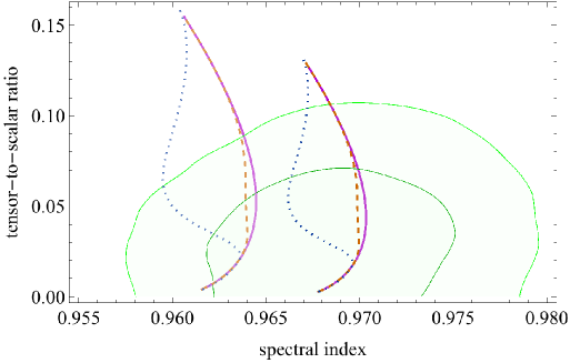
Using the method described in Appendix A, we calculated the prediction of , which is shown in Fig. 2. We see that the predicted values for and nicely fit the observational results, especially for . Let us discuss a limiting case with , and . In this limit the canonical field is given by
| (3.27) |
In terms of the canonical field, the potential reduces to Eq. (3.13) and hence the same prediction (3.14) is recovered. The field value of at the -folding number is given by
| (3.28) |
For consistency of the approximation, we should have
| (3.29) |
When these conditions are not satisfied, e.g. with large and nonzero , there are sizable corrections to the above potential. An example of prediction for such a case with is shown in Fig. 2.
Let us comment on the meaning of the parameters and curvature of the Kähler manifold specified by eq. (3.19). parametrizes deformation from the original -term attractor model (3.8). In the absence of , defines the curvature of the Kähler manifold (3.2), and controls the way the inflaton is normalized. This, in turn, determines the slope of the potential and hence the tensor-to-scalar ratio. Meanwhile, controls the overall normalization of the potential. In the presence of , the Kähler curvature now depends on the field value as well as the parameters , , and . The exact expression is too long to be displayed here, but we can discuss some limits. First of all, the limit or reduces to the undeformed result, . This reflects the fact that the effects of the deformation is minor in the large field limit. The opposite limit leads to . However, in this limit, the tensor-to-scalar ratio is approximately independent of , as discussed above. Thus, with general , the Kähler curvature is not directly related to the inflationary observables.
3.3 Stabilization of other fields
As mentioned before, there are additional fields and , which must be stabilized during inflation. Here, we consider the following superpotential,
| (3.30) |
The masses of and in the canonical basis during inflation are given by [see Eq. (2.18)]
| (3.31) |
If we naively extend the Kähler potential (3.21) by introducing additional fields,
| (3.32) |
masses of and become
| (3.33) |
Here and hereafter, our main interest is the attractor regime, so we have neglected and assumed . Note that in the non-canonical basis, exponentially grows as as seen from Eq. (3.28). Thus we find that
| (3.34) |
It means that their masses become at least times larger during the last -foldings, and that they easily exceed the Planck scale. This situation is similar to that of the polynomial models described in Sec. 2.
The difficulty described above can be alleviated if we introduce the following terms in addition to Eq. (3.32),
| (3.35) |
In this case, masses from -term potential read
| (3.36) |
Note that the exponentially large factor is canceled by . In order to avoid the appearance of super-Planckian masses before the end of inflation, we require the following condition,
| (3.37) |
It is also necessary to check that the -term masses (3.36) actually stabilize and against a negative contribution from -term potential and the Hubble friction. Due to the additional terms in Eqs. (3.32) and (3.35), the -term potential is modified as follows,
| (3.38) |
which leads to the following masses for and in the canonical basis,
| (3.39) |
Two fields are stabilized if the total masses and remain larger than during inflation. Since the negative contribution dominates over for , it is sufficient to require that . From this condition, we find
| (3.40) |
Furthermore, some parameters are constrained by the requirement that they explain the amplitude of the observed power spectrum of the curvature perturbation [5],
| (3.41) |
Combining Eqs. (3.37), (3.40) and (3.41), we obtain
| (3.42) |
where .
The condition (3.42) is easily satisfied for . On the other hand, if the power exponent of in Eq. (3.35) is some integer, the value of is constrained, and its smallest value is . In this case, larger values for and/or smaller values for are required in order to satisfy the condition (3.41), but cannot be arbitrarily large since it easily conflicts with the constraint (3.42). Furthermore, a larger value of leads to a large tensor to scalar ratio [see Eq. (3.14)], which also conflicts with observational results.
4 Kähler potential for -term pole inflation
The -attractor is characterized by a second order pole in the coefficient of the inflaton kinetic term [12]. Its prediction is and . This is generalized to poles of arbitrary order [12, 20, 21]. When the inflaton field has a pole of order in the kinetic term, we redefine the origin of the field so that the pole coincides with the origin. Then, we have the following inflaton Lagrangian,
| (4.1) |
For the sign of the kinetic term to be physical, with even has to be positive. For odd , if is negative, we redefine and , and drop the primes. Thus, without loss of generality, we can assume and . The parameter of the -attractor is related to as . If the potential has a positive finite value at its origin and is smoothly connected to a vacuum,#10#10#10 For more general cases in which the potential also has a pole at , the canonical potential becomes an exponential term (power-law inflation) or monomial (chaotic inflation) [49, 21]. In this paper, we are mainly interested in plateau-type potentials, and do not consider singular potentials. See Sec. 4.1, however, for a pole with a small coefficient as a small shift-symmetry breaking effect. the spectral index and tensor-to-scalar ratio are given by [12]
| (4.2) |
where is rescaled by the ratio of the constant and linear terms in , (see Eq. (4.6) below where and are introduced).
In this section, we derive the form of Kähler potential leading to pole inflation of order in the case of -term inflation. In Ref. [20], the form of Kähler potential is studied for with higher order pole corrections. We discuss general , and derive the Kähler potential in terms of the ordinary U(1) charged field . We investigate effects of higher order poles in the next subsection.
Using the general prescription given in Ref. [16], we can construct any monotonically increasing potential. The canonical inflaton potential for pole inflation is known [20], so we can construct Kähler potential leading to the potential. Though equivalent, we focus in the following analysis more on the variable having a pole in the kinetic term because it is the essence of pole inflation.
To derive the conditions on the Kähler potential, it is useful to deal with a shift-symmetric field because derivative of with respect to and its conjugate are same,
| (4.3) |
Similar relations hold for higher derivatives. We therefore introduce a real variable as in Ref. [16], and the Kähler potential is effectively a function of a single variable, .
This does not necessarily coincide with introduced above, so . The coefficient of the kinetic term is given by the Kähler metric, so we require
| (4.4) |
where prime denotes differentiation with respect to . Since transforms by a constant shift under U(1) transformation, the -term potential is given by
| (4.5) |
Therefore, should be a regular function of at the origin. Expanding it up to a first order, we obtain
| (4.6) |
The relative sign of and should be negative because otherwise inflaton keeps roll down to the origin, and inflation does not end. Combining Eqs. (4.4) and (4.6), we obtain
| (4.7) |
where we neglect an integration constant which can be absorbed by the shift of . Integrating the above equation, we find the following form for the Kähler potential,
| (4.8) |
where , and is an integration constant. For , we reproduce Eqs. (3.8) or (3.9) depending on the sign of (or ) with identification , , and .
Although we can define the transformation of or corresponding to the shift of canonical inflaton , we do not find a simple formula or interpretation for the cases with .
As demonstrated in Sec. 2.2 and Sec. 3.3, we can introduce fields for anomaly cancellation and stabilize them during inflation. It is a straightforward generalization, so we do not repeat it here.
4.1 Symmetry breaking effects
Next, we consider effects of higher order poles as symmetry breaking effects [20],
| (4.9) |
where without loss of generality, and we assume during inflation because otherwise the effect of pole of order can be negligible and the previous discussion applies with substitution . We treat the term as a perturbation. The observational effect on due to this perturbation is given by the following shifts [20]
| (4.10) | ||||
| (4.11) |
where and .
Due to the existence of higher order poles, Eq. (4.4) is replaced with
| (4.12) |
Up to the first order in , the additional term in the Kähler potential is
| (4.13) |
In the case of -attractor (), this reduces to
| (4.14) |
Thus, higher order terms with respect to in the Kähler potential can be interpreted as symmetry breaking terms.
One may also consider a pole in the potential suppressed by a small number as another source of shift symmetry breaking. In this case, Eq. (4.6) is replaced with
| (4.15) |
where we assume the first term is subdominant to the second term during observable length of inflation. This leads to -th and -th order poles in the potential at the first order of . The latter is subdominant assuming the term is dominant in Eq. (4.15) during inflation. Such a term affects and [21],
| (4.16) | ||||
| (4.17) |
where measures the relative magnitude of the singular term in the potential. Combining Eq. (4.15) with Eq. (4.4), we can similarly obtain the correction to the Kähler potential up to a first order in ,
| (4.18) |
In the case of -attractor (), this reduces to
| (4.19) |
These are also higher order terms in . The similarity to the case of a higher order pole in the kinetic term can be understood as follows. In Eq. (4.15), one can redefine the field as . This eliminates the pole in the potential, but it induces a pole in the kinetic term. Thus, to the first order of , one can map the Lagrangian to the form of Eq. (4.9). In this way, small perturbation as a form of higher order terms in the Kähler potential are equivalent to the shift symmetry breaking effect in terms of the canonical inflaton field , which can be interpreted either as an additional pole in the kinetic term or as a pole in the potential in terms of an intermediate field .
5 Conclusion and discussions
In this paper we have tried to construct a concrete model of -term inflation based on attractor models. First, we have shown that simple models of -term chaotic inflation do not fit the current data, unfortunately. In addition, we have pointed out that the effective masses of and during inflation is exponentially large and typically beyond the Planck scale, which might destroy the validity of the calculations due to quantum gravity effects. As shown explicitly, higher order corrections to the Kähler potential improve the fit to the data and succeed in suppressing masses of the additional fields adequately. However, without symmetry reason, these corrections are uncontrollable.
Then, we have revisited the -term inflationary attractor models in this paper. These attractor models can be realized in the context of pole inflation with a second order pole in the kinetic term. However, we have seen the limitation on the structure of Kähler potential for -term inflationary attractor models. Actually, it is not automatically guaranteed that a sufficiently flat potential is obtained even if one specifies a Kähler potential which leads to a second order pole in the kinetic term. This is because the -term potential is also determined by the Kähler potential. We have extended the models in order to construct a workable example, in which Kähler potential is defined in Coulomb phase as well as in Higgs phase, gauge anomaly is cancelled and other required fields including the stabilizer field are stabilized during inflation. These can be viewed as a first step of UV completing the -term attractor models. For these models with plateau type potentials, understanding the origin of shift symmetry for canonical inflaton is important. We pointed out that it is a symmetry under the transformation for the -attractor (pole inflation with ) case.
Finally let us discuss the reheating of the universe in our model (3.21). In particular, let us consider the case of , in which the global potential minimum is given by (3.25) and .#11#11#11At the potential minimum, the Kähler metric becomes zero and the physical mass of diverges. To avoid this, we may introduce a small correction, e.g., . Although it can mildly affect the Kähler potential (3.35) required for safely stabilizing the inflationary path, the qualitative discussion remains intact. After inflation, inflaton begins to oscillate around the minimum of the potential. The inflaton and gauge boson masses around the potential minimum are given by
| (5.1) |
Since SUSY is preserved at the minimum, the masses of the inflaton and the gauge boson, which are both members of a massive gauge supermultiplet, are same. Inflaton does not decay into gauge bosons or gauginos for the kinematical reason. To reheat the standard model sector, we may introduce a (small) kinetic mixing between the gauge bosons of the U(1) and the standard model hypercharge U(1)Y. Then the inflaton or hidden gauge bosons decay into the standard model U(1)Y gauge boson pair through the mixing. The case of is similar, but the cosmic string may be formed. When , the inflaton is massless at the vacuum, and reheating becomes nontrivial.
Acknowledgments
We would like to thank J. Yokoyama for his collaboration and useful comments at the initial stage of the present work. This work was supported by the Grant-in-Aid for Scientific Research on Scientific Research (No. 2610619 [TT]), Scientific Research A (No.26247042 [KN]), Young Scientists B (No.26800121 [KN]), Innovative Areas (No.26104009 [KN], No.15H05888 [KN, MY]), Scientific Research Nos. 25287054[MY], 26610062[MY]. KS and TT are also supported by the Grant-in-Aid for JSPS Fellows.
Appendix A Slow-roll inflation in non-canonical basis
Let us consider the Lagrangian with a non-canonical scalar field
| (A.1) |
The canonical field is
| (A.2) |
but often this integral cannot be analytically performed. Thus it may be convenient to consider the inflaton dynamics in a non-canonical basis.
The equation of motion is
| (A.3) |
The subscript denotes the derivative with respect to . The Friedmann equation is
| (A.4) |
In the slow-roll limit, we have
| (A.5) | |||
| (A.6) |
The slow-roll consistency conditions are
| (A.7) |
where
| (A.8) |
The slow-roll equation is rewritten in terms of the -folding as
| (A.9) |
so is calculated as
| (A.10) |
where and are the field values at the end of inflation and at -foldings before that. According to the formalism [50, *Sasaki:1995aw, *Sasaki:1998ug, *Lyth:2004gb], the curvature perturbation is evaluated as
| (A.11) |
Note that it is the canonical field , not , that obtains long wave quantum fluctuation of during inflation:
| (A.12) |
Then we obtain the dimensionless power spectrum of the curvature perturbation as
| (A.13) |
The scalar spectral index is given by
| (A.14) |
The tensor-to-scalar ratio is given by
| (A.15) |
Appendix B Generic scalar potential in -term inflation
In this section we explicitly construct a “generic scalar potential” as an explicit realization of Ref. [16] in terms of Higgs fields and . In contrast to the original model, it is well-defined at and . Let us consider the following Kähler potential
| (B.1) |
In the small field limit , this is expanded as , but in the large field limit the behavior is significantly modified. From this Kähler potential we obtain
| (B.2) | |||
| (B.3) |
Note that the Kähler metric is regular at for . The fields are canonically normalized in the limit for . The -term potential for with is given by
| (B.4) |
Let us consider the limit . If are non-zero, it is easy to see that the canonical field becomes . Actually for , the kinetic term becomes
| (B.5) |
Therefore we have . Then from Eq. (B.4) we obtain the -term potential just as polynomial of ,
| (B.6) |
where we assumed and neglected with and . Thus we obtain a polynomial type potential. It is obvious that we can also obtain more general form by choosing appropriately.
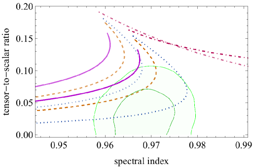
To illustrate impacts of this type of model, we solved the dynamics of assuming . For numerical calculation we take , and . The result is shown in Fig. 3 for , and . For each line, we varied within the range satisfying for the whole last 60 -foldings.
The stability of and during inflation is a nontrivial issue also in this model, but we can arrange the superpotential and Kähler potential so that they are stabilized at the origin while avoiding too large masses in a similar fashion to that of Sec. 2.2.
References
- [1] K. Sato and J. Yokoyama, “Inflationary cosmology: First 30+ years,” Int. J. Mod. Phys. D24 no. 11, (2015) 1530025.
- [2] WMAP Collaboration, C. L. Bennett et al., “Nine-Year Wilkinson Microwave Anisotropy Probe (WMAP) Observations: Final Maps and Results,” Astrophys. J. Suppl. 208 (2013) 20, arXiv:1212.5225 [astro-ph.CO].
- [3] WMAP Collaboration, G. Hinshaw et al., “Nine-Year Wilkinson Microwave Anisotropy Probe (WMAP) Observations: Cosmological Parameter Results,” Astrophys. J. Suppl. 208 (2013) 19, arXiv:1212.5226 [astro-ph.CO].
- [4] Planck Collaboration, P. A. R. Ade et al., “Planck 2015 results. XIII. Cosmological parameters,” arXiv:1502.01589 [astro-ph.CO].
- [5] Planck Collaboration, P. A. R. Ade et al., “Planck 2015 results. XX. Constraints on inflation,” arXiv:1502.02114 [astro-ph.CO].
- [6] R. Kallosh, A. Linde, and D. Roest, “Universal Attractor for Inflation at Strong Coupling,” Phys. Rev. Lett. 112 no. 1, (2014) 011303, arXiv:1310.3950 [hep-th].
- [7] C. Pallis, “Linking Starobinsky-Type Inflation in no-Scale Supergravity to MSSM,” JCAP 1404 (2014) 024, arXiv:1312.3623 [hep-ph].
- [8] G. F. Giudice and H. M. Lee, “Starobinsky-like inflation from induced gravity,” Phys. Lett. B733 (2014) 58–62, arXiv:1402.2129 [hep-ph].
- [9] C. Pallis, “Induced-Gravity Inflation in no-Scale Supergravity and Beyond,” JCAP 1408 (2014) 057, arXiv:1403.5486 [hep-ph].
- [10] R. Kallosh, A. Linde, and D. Roest, “Large field inflation and double -attractors,” JHEP 08 (2014) 052, arXiv:1405.3646 [hep-th].
- [11] R. Kallosh, A. Linde, and D. Roest, “The double attractor behavior of induced inflation,” JHEP 09 (2014) 062, arXiv:1407.4471 [hep-th].
- [12] M. Galante, R. Kallosh, A. Linde, and D. Roest, “Unity of Cosmological Inflation Attractors,” Phys. Rev. Lett. 114 no. 14, (2015) 141302, arXiv:1412.3797 [hep-th].
- [13] J. J. M. Carrasco, R. Kallosh, A. Linde, and D. Roest, “Hyperbolic geometry of cosmological attractors,” Phys. Rev. D92 no. 4, (2015) 041301, arXiv:1504.05557 [hep-th].
- [14] R. Kallosh and A. Linde, “Universality Class in Conformal Inflation,” JCAP 1307 (2013) 002, arXiv:1306.5220 [hep-th].
- [15] J. Ellis, D. V. Nanopoulos, and K. A. Olive, “Starobinsky-like Inflationary Models as Avatars of No-Scale Supergravity,” JCAP 1310 (2013) 009, arXiv:1307.3537 [hep-th].
- [16] S. Ferrara, R. Kallosh, A. Linde, and M. Porrati, “Minimal Supergravity Models of Inflation,” Phys. Rev. D88 no. 8, (2013) 085038, arXiv:1307.7696 [hep-th].
- [17] R. Kallosh, A. Linde, and D. Roest, “Superconformal Inflationary -Attractors,” JHEP 11 (2013) 198, arXiv:1311.0472 [hep-th].
- [18] J. J. M. Carrasco, R. Kallosh, and A. Linde, “-Attractors: Planck, LHC and Dark Energy,” JHEP 10 (2015) 147, arXiv:1506.01708 [hep-th].
- [19] M. D. Pollock and D. Sahdev, “Pole Law Inflation in a Theory of Induced Gravity,” Phys. Lett. B222 (1989) 12.
- [20] B. J. Broy, M. Galante, D. Roest, and A. Westphal, “Pole inflation – Shift symmetry and universal corrections,” JHEP 12 (2015) 149, arXiv:1507.02277 [hep-th].
- [21] T. Terada, “Generalized Pole Inflation: Hilltop, Natural, and Chaotic Inflationary Attractors,” arXiv:1602.07867 [hep-th].
- [22] A. Mazumdar and J. Rocher, “Particle physics models of inflation and curvaton scenarios,” Phys. Rept. 497 (2011) 85–215, arXiv:1001.0993 [hep-ph].
- [23] M. Yamaguchi, “Supergravity based inflation models: a review,” Class. Quant. Grav. 28 (2011) 103001, arXiv:1101.2488 [astro-ph.CO].
- [24] T. Terada, Inflation in Supergravity with a Single Superfield. PhD thesis, Tokyo U., 2015. arXiv:1508.05335 [hep-th]. http://inspirehep.net/record/1388860/files/arXiv:1508.05335.pdf.
- [25] E. J. Copeland, A. R. Liddle, D. H. Lyth, E. D. Stewart, and D. Wands, “False vacuum inflation with Einstein gravity,” Phys. Rev. D49 (1994) 6410–6433, arXiv:astro-ph/9401011 [astro-ph].
- [26] M. Kawasaki, M. Yamaguchi, and T. Yanagida, “Natural chaotic inflation in supergravity,” Phys. Rev. Lett. 85 (2000) 3572–3575, arXiv:hep-ph/0004243 [hep-ph].
- [27] M. Kawasaki, M. Yamaguchi, and T. Yanagida, “Natural chaotic inflation in supergravity and leptogenesis,” Phys. Rev. D63 (2001) 103514, arXiv:hep-ph/0011104 [hep-ph].
- [28] H. Murayama, H. Suzuki, T. Yanagida, and J. Yokoyama, “Chaotic inflation and baryogenesis in supergravity,” Phys. Rev. D50 (1994) 2356–2360, arXiv:hep-ph/9311326 [hep-ph].
- [29] P. Binetruy and G. R. Dvali, “D term inflation,” Phys. Lett. B388 (1996) 241–246, arXiv:hep-ph/9606342 [hep-ph].
- [30] E. Halyo, “Hybrid inflation from supergravity D terms,” Phys. Lett. B387 (1996) 43–47, arXiv:hep-ph/9606423 [hep-ph].
- [31] K. Kadota and M. Yamaguchi, “D-term chaotic inflation in supergravity,” Phys. Rev. D76 (2007) 103522, arXiv:0706.2676 [hep-ph].
- [32] T. Kawano, “Chaotic D-term inflation,” Prog. Theor. Phys. 120 (2008) 793–795, arXiv:0712.2351 [hep-th].
- [33] K. Kadota, T. Kawano, and M. Yamaguchi, “New D-term chaotic inflation in supergravity and leptogenesis,” Phys. Rev. D77 (2008) 123516, arXiv:0802.0525 [hep-ph].
- [34] S. Ferrara, R. Kallosh, A. Linde, and M. Porrati, “Higher Order Corrections in Minimal Supergravity Models of Inflation,” JCAP 1311 (2013) 046, arXiv:1309.1085 [hep-th].
- [35] H. Abe, Y. Sakamura, and Y. Yamada, “Massive vector multiplet inflation with Dirac-Born-Infeld type action,” Phys. Rev. D91 no. 12, (2015) 125042, arXiv:1505.02235 [hep-th].
- [36] C. Destri, H. J. de Vega, and N. G. Sanchez, “MCMC analysis of WMAP3 and SDSS data points to broken symmetry inflaton potentials and provides a lower bound on the tensor to scalar ratio,” Phys. Rev. D77 (2008) 043509, arXiv:astro-ph/0703417 [astro-ph].
- [37] K. Nakayama, F. Takahashi, and T. T. Yanagida, “Polynomial Chaotic Inflation in the Planck Era,” Phys. Lett. B725 (2013) 111–114, arXiv:1303.7315 [hep-ph].
- [38] K. Nakayama, F. Takahashi, and T. T. Yanagida, “Polynomial Chaotic Inflation in Supergravity,” JCAP 1308 (2013) 038, arXiv:1305.5099 [hep-ph].
- [39] R. Kallosh and A. Linde, “New models of chaotic inflation in supergravity,” JCAP 1011 (2010) 011, arXiv:1008.3375 [hep-th].
- [40] R. Kallosh, A. Linde, and T. Rube, “General inflaton potentials in supergravity,” Phys. Rev. D83 (2011) 043507, arXiv:1011.5945 [hep-th].
- [41] T. Li, Z. Li, and D. V. Nanopoulos, “Helical Phase Inflation and Monodromy in Supergravity Theory,” Adv. High Energy Phys. 2015 (2015) 397410, arXiv:1412.5093 [hep-th].
- [42] Z. Komargodski and N. Seiberg, “Comments on the Fayet-Iliopoulos Term in Field Theory and Supergravity,” JHEP 06 (2009) 007, arXiv:0904.1159 [hep-th].
- [43] Z. Komargodski and N. Seiberg, “Comments on Supercurrent Multiplets, Supersymmetric Field Theories and Supergravity,” JHEP 07 (2010) 017, arXiv:1002.2228 [hep-th].
- [44] K. R. Dienes and B. Thomas, “On the Inconsistency of Fayet-Iliopoulos Terms in Supergravity Theories,” Phys. Rev. D81 (2010) 065023, arXiv:0911.0677 [hep-th].
- [45] P. Binetruy, G. Dvali, R. Kallosh, and A. Van Proeyen, “Fayet-Iliopoulos terms in supergravity and cosmology,” Class. Quant. Grav. 21 (2004) 3137–3170, arXiv:hep-th/0402046 [hep-th].
- [46] F. Catino, G. Villadoro, and F. Zwirner, “On Fayet-Iliopoulos terms and de Sitter vacua in supergravity: Some easy pieces,” JHEP 01 (2012) 002, arXiv:1110.2174 [hep-th].
- [47] M. Dine, N. Seiberg, and E. Witten, “Fayet-Iliopoulos Terms in String Theory,” Nucl. Phys. B289 (1987) 589.
- [48] C. Wieck and M. W. Winkler, “Inflation with Fayet-Iliopoulos Terms,” Phys. Rev. D90 no. 10, (2014) 103507, arXiv:1408.2826 [hep-th].
- [49] M. Rinaldi, L. Vanzo, S. Zerbini, and G. Venturi, “Inflationary quasiscale-invariant attractors,” Phys. Rev. D93 no. 2, (2016) 024040, arXiv:1505.03386 [hep-th].
- [50] A. A. Starobinsky, “Multicomponent de Sitter (Inflationary) Stages and the Generation of Perturbations,” JETP Lett. 42 (1985) 152–155. [Pisma Zh. Eksp. Teor. Fiz.42,124(1985)].
- [51] M. Sasaki and E. D. Stewart, “A General analytic formula for the spectral index of the density perturbations produced during inflation,” Prog. Theor. Phys. 95 (1996) 71–78, arXiv:astro-ph/9507001 [astro-ph].
- [52] M. Sasaki and T. Tanaka, “Superhorizon scale dynamics of multiscalar inflation,” Prog. Theor. Phys. 99 (1998) 763–782, arXiv:gr-qc/9801017 [gr-qc].
- [53] D. H. Lyth, K. A. Malik, and M. Sasaki, “A General proof of the conservation of the curvature perturbation,” JCAP 0505 (2005) 004, arXiv:astro-ph/0411220 [astro-ph].