On the inconsistency of $\ell_{1}$-penalised sparse precision matrix estimation

Abstract

Various $\ell_{1}$-penalised estimation methods such as graphical lasso and CLIME are widely used for sparse precision matrix estimation. Many of these methods have been shown to be consistent under various quantitative assumptions about the underlying true covariance matrix. Intuitively, these conditions are related to situations where the penalty term will dominate the optimisation. In this paper, we explore the consistency of $\ell_{1}$-based methods for a class of sparse latent variable -like models, which are strongly motivated by several types of applications. We show that all $\ell_{1}$-based methods fail dramatically for models with nearly linear dependencies between the variables. We also study the consistency on models derived from real gene expression data and note that the assumptions needed for consistency never hold even for modest sized gene networks and $\ell_{1}$-based methods also become unreliable in practice for larger networks.

1 INTRODUCTION

Estimating the sparse precision matrix, i.e. the inverse covariance matrix, from data is a very widely used method for exploring the dependence structure of continuous variables. The motivation for the approach stems from the fact that for a Gaussian Markov random field model, zeros in the precision matrix translate exactly to absent edges in the corresponding undirected Gaussian graphical model, thus being informative about the marginal and conditional independence relationships among the variables.

The full $p$-dimensional covariance matrix contains $p(p+1)/2$ parameters, making its accurate estimation from limited data difficult. Additionally, the structure learning requires the inverse of the covariance, and matrix inversion is in general a very fragile operation. To make the problem tractable, some form of regularisation is typically needed. Direct optimisation of the sparse structure would easily lead to very difficult combinatorial optimisation problems. To avoid these computational difficulties, several convex $\ell_{1}$-penalty-based approaches have been proposed. Popular examples include $\ell_{1}$-penalised maximum likelihood estimation (Meinshausen and Bühlmann, 2006), which also forms the basis for the highly popular graphical lasso (glasso) algorithm (Friedman et al., 2008). $\ell_{1}$ regularisation has also been used for example in a non-probabilistic alternative with linear-programming-based constrained $\ell_{1}$ minimisation (CLIME) algorithm of Cai et al. (2011).

At the heart of the optimisation problems considered by all these methods is a term depending on the $\ell_{1}$ norm of the estimated precision matrix. $\ell_{1}$-penalisation-based approaches such as lasso are popular for sparse regression, but they have a known weakness: in addition to promoting sparsity they also push true non-zero elements toward zero (Zhao and Yu, 2006). In the context of precision matrix estimation this effect would be expected to be especially strong when some elements of the precision matrix are large, which happens for scaled covariance matrices when the covariance matrix becomes ill-conditioned. This phenomenon occurs frequently under the circumstances where some of the variables are nearly linearly dependent.

In this paper we demonstrate a drastic failure of the $\ell_{1}$ penalised sparse covariance estimation methods for a class of models that have a linear latent variable structure where some variables depend linearly on others. For such models even in the limit of infinite data, popular $\ell_{1}$ penalised methods cannot yield results that are significantly better than based on random guessing on any setting of the regularisation parameter. Yet these models have a very clear sparse structure that becomes obvious from the empirical precision matrix with an increasing $n$.

Given the huge popularity and success of linear models in modelling data, structures like the one considered in our work are natural for various real world data sets. Motivated by our discovery, we also explore the inconsistency of $\ell_{1}$ penalised methods on models derived from real gene expression data and find them poorly suited for such applications.

2 STRUCTURE LEARNING OF GAUSSIAN GRAPHICAL MODELS

2.1 BACKGROUND

We start with a quick recap on the basics of Gaussian graphical models in order to formulate the problem of structure learning. For a more comprehensive treatment of the subject, we refer to (Whittaker 1990; Lauritzen 1996). Let $\mathbf{X}=(X_{1},\ldots,X_{p})^{\prime}$ denote a random vector following a multivariate normal distribution with zero mean and a covariance matrix $\mathbf{\Sigma}$, $\mathbf{X}\sim N_{p}(\mathbf{0},\mathbf{\Sigma})$. Let $G=(V,E)$ be an undirected graph, where the $V=\{1,\ldots,p\}$ is the set of nodes and $E\subset V\times V$ stands for the set of edges. The nodes in the graph represent the random variables in the vector $\mathbf{X}$ and absences of the edges in the graph correspond conditional independence assertions between these variables. More in detail, we have that $(i,j)\not\in E$ and $(j,i)\not\in E$ if and only if $X_{i}$ is conditionally independent of $X_{j}$ given the remaining variables in $\mathbf{X}$.

In the multivariate normal setting, there is a one-to-one correspondence between the missing edges in the graph and the off-diagonal zeros of the precision matrix $\mathbf{\Omega}=\mathbf{\Sigma}^{-1}$, that is, $\omega_{ij}=0\Leftrightarrow X_{i}\mathchoice{\mathrel{\hbox to0.0pt{$\displaystyle\perp$\hss}\mkern 2.0mu{\displaystyle\perp}}}{\mathrel{\hbox to0.0pt{$\textstyle\perp$\hss}\mkern 2.0mu{\textstyle\perp}}}{\mathrel{\hbox to0.0pt{$\scriptstyle\perp$\hss}\mkern 2.0mu{\scriptstyle\perp}}}{\mathrel{\hbox to0.0pt{$\scriptscriptstyle\perp$\hss}\mkern 2.0mu{\scriptscriptstyle\perp}}}X_{j}\ |\mathbf{X}\setminus\{X_{i},X_{j}\}$ (see, for instance, Lauritzen 1996, p. 129). Given an undirected graph $G$, a Gaussian graphical model is defined as the collection of multivariate normal distributions for $\mathbf{X}$ satisfying the conditional independence assertions implied by the graph $G$.

Assume we have a complete (no missing observations) i.i.d. sample $\mathbf{x}=(\mathbf{x}_{1},\ldots,\mathbf{x_{n}})$ from the distribution $N_{p}(\mathbf{0},\mathbf{\Sigma})$. Based on the sample $\mathbf{x}$, our goal in structure learning is to find the graph $G$, or equivalently, learn the zero-pattern of $\mathbf{\Omega}$. The usual assumption is that the underlying graph is sparse. A naive estimate for $\mathbf{\Omega}$ by inverting the sample covariance matrix is practically never truly sparse for any real data. Furthermore, if $n<p$ the sample covariance matrix is rank-deficient and thus not even invertible.

One common approach to overcome these problems is to impose an additional $\ell_{1}$-penalty on the elements of $\mathbf{\Omega}$ when estimating it. This kind of regularisation effectively forces some of the elements of $\mathbf{\Omega}$ to zero, thus resulting in sparse solutions. In the context of regression models, this method applied on the regression coefficients goes by the name of lasso (Tibshirani, 1996). There exists a wide variety of methods making use of $\ell_{1}$-regularisation in the setting of Gaussian graphical model structure learning (Yuan and Lin 2007; Meinshausen and Bühlmann 2006; Banerjee et al. 2008; Friedman et al. 2008; Peng et al. 2009; Cai et al. 2011; Hsieh et al. 2014).

2.2 $\ell_{1}$-REGULARISED METHODS

In this section we provide a brief review of selected examples of different types of $\ell_{1}$-penalised methods.

2.2.1 Glasso

We begin with the widely used graphical lasso-algorithm (glasso) by Friedman et al. (2008). Glasso-method maximises an objective function consisting of the Gaussian log-likelihood and an $\ell_{1}$-penalty:

$$\log\det(\mathbf{\Omega})-\textnormal{trace}(\mathbf{\Omega S})-\lambda||\mathbf{\Omega}||_{1},$$ (1)

where $\mathbf{S}$ denotes the sample covariance matrix and $\lambda>0$ is the regularisation parameter controlling the sparsity of the solution. The $\ell_{1}$ penalty, $||\boldsymbol{\Omega}||_{1}=\sum_{i,j}|\omega_{ij}|$, is applied on all the elements of $\boldsymbol{\Omega}$, but the variant where the diagonal elements are omitted is also common. The objective function (1) is maximised over all positive definite matrices $\mathbf{\Omega}$ and the optimisation is carried out in practice using a block-wise coordinate descent.

2.2.2 CLIME

Cai et al. (2011) approach the problem of sparse precision matrix estimation from a slightly different perspective. Their CLIME-method (Constrained $\ell_{1}$-minimisation for Inverse Matrix Estimation) seeks matrices $\boldsymbol{\Omega}$ with a minimal $\ell_{1}$-norm under the following constraint

$$|\mathbf{S}\boldsymbol{\Omega}-\mathbf{I}|_{\infty}\leq\lambda,$$ (2)

where $\lambda$ is the tuning parameter and $|\mathbf{A}|_{\infty}=\max_{i,j}|a_{ij}|$ is the element-wise maximum. The optimisation problem $\min_{\boldsymbol{\Omega}}||\boldsymbol{\Omega}||_{1}$ subject to the constraint (2) does not explicitly force the solution to be symmetric, which is resolved by picking from estimated values $\omega_{ij}$ and $\omega_{ji}$ the one with a smaller magnitude into the final solution. In practice, the optimisation problem is decomposed over variables into $p$ sub-problems which are then efficiently solved using linear programming.

2.2.3 SCIO

Liu and Luo (2015) introduced recently a method called Sparse Column-wise Inverse Operator (SCIO). The SCIO-method decomposes the estimation of $\boldsymbol{\Omega}$ into a following smaller problems

$$\min_{\boldsymbol{\beta}_{i}\in\mathbb{R}^{p}}\left\{\frac{1}{2}\boldsymbol{\beta}_{i}^{T}\mathbf{S}\boldsymbol{\beta}_{i}-\textbf{e}_{i}^{T}\boldsymbol{\beta}_{i}+\lambda||\boldsymbol{\beta}_{i}||_{1}\right\},$$

where $\mathbf{S}$ and $\lambda$ are defined as before and $\textbf{e}_{i}$ is an $i$:th standard unit vector. The regularisation parameter $\lambda$ can in general vary with $i$ but this is omitted in our notation. The solutions $\hat{\boldsymbol{\beta}}_{i}$ form the columns for the estimate of $\boldsymbol{\Omega}$. Also for SCIO, the symmetry of the resulting precision matrix must be forced, and this is done as described in the case of CLIME.

2.3 ALTERNATIVE METHODS

2.3.1 The naive approach

In addition to the above-mentioned $\ell_{1}$-penalised methods, we consider two alternative approaches. In a ”naive” approach, we simply take the sample covariance matrix, invert it, and then threshold the resulting matrix to obtain a sparse estimate for the precision matrix. The threshold value is chosen using the ground truth graph so that the naive estimator will have as many non-zero entries as there are edges in the true graph. Setting the threshold value according to the ground truth is of course unrealistic, however, it is nevertheless interesting to compare the accuracy of this simple procedure to the performance of the more refined $\ell_{1}$-methods, when also their tuning parameters are chosen in a similar fashion.

2.3.2 FMPL

Lastly, we consider a Bayesian approach which is based on finding a graph with a highest fractional marginal pseudo-likelihood (FMPL) by Leppä-aho et al. (2016). The fractional marginal pseudo-likelihood is an approximation of the marginal likelihood and it has been shown to be a consistent scoring function in the sense that the true graph maximises it as the sample size tends to infinity, under the assumption that data are generated from a multivariate normal distribution. The FMPL-score decomposes over variables and in practice, the method identifies optimal Markov blankets for each of the variables, which are then combined into a proper undirected graph using any of the three different schemes commonly employed in graphical model learning: OR, AND and HC.

2.4 MODEL SELECTION CONSISTENCY

The assumptions required for a consistent model selection with an $\ell_{1}$-penalised Gaussian log-likelihood have been studied, for instance, in Ravikumar et al. (2011). The authors provide a number of conditions in the multivariate normal model that are sufficient for the recovery of the zero pattern of the true precision matrix $\boldsymbol{\Omega}^{*}$ with a high probability when the sample size is large. For our purposes, the most relevant condition is the following:

Assumption 1.

There exists $\alpha\in(0,1],$ such that

$$\gamma:=||\Gamma_{S^{C}S}{(\Gamma_{SS})}^{-1}||_{\infty}\leq 1-\alpha.$$ (3)

Here $S\subset V\times V$ is a set defining the support of $\boldsymbol{\Omega}^{*}$, that is, the non-zero elements of $\boldsymbol{\Omega}^{*}$ (diagonal and the elements corresponding to the edges in the graphical model) and $S^{C}$ refers to the complement of $S$ in $V\times V$. The $\Gamma$ term is defined via Kronecker product $\otimes$ as $\Gamma=(\boldsymbol{\Omega}^{*})^{-1}\otimes(\boldsymbol{\Omega}^{*})^{-1}\in\mathbb{R}^{p^{2}\times p^{2}}$ and $\Gamma_{AB}$ refers to the specific rows and columns of $\Gamma$ indexed by $A\subset V\times V$ and $B\subset V\times V$, respectively. The norm in the equation is defined as $||A||_{\infty}=\max_{j}\sum_{i}|a_{ij}|$.

The above result applies to glasso. However, a quite similar result was presented for SCIO in Liu and Luo (2015):

Assumption 2.

There exists $\alpha\in(0,1),$ such that

$$\max_{1\leq i\leq p}||\boldsymbol{\Sigma}^{*}_{\textbf{s}_{i}^{C}\textbf{s}_{i}}{(\boldsymbol{\Sigma}^{*}_{\textbf{s}_{i}\textbf{s}_{i}})}^{-1}||_{\infty}\leq 1-\alpha.$$

Here $\boldsymbol{\Sigma}^{*}=(\boldsymbol{\Omega}^{*})^{-1}$ and $\textbf{s}_{i}=\{j\in\{1,\ldots,p\}\ |\ (\boldsymbol{\Omega}^{*})_{ij}\neq 0\}$. Assumption 2 under the multivariate normality guarantees that the support of $\boldsymbol{\Omega}^{*}$ is recovered by SCIO with a high probability as the sample size gets large.

3 LATENT VARIABLE LIKE MODELS INDUCE INCONSISTENCY WITH $\ell_{1}$-PENALISATION

Methods for sparse precision matrix estimation generally depend on an objective function (such as log-likelihood) and a penalty function or regulariser, which in a Bayesian setting is usually represented by the prior. The ideal penalty function for many problems would be the $\ell_{0}$ “norm” counting the number of non-zero elements: $||x||_{0}=\#\{i|x_{i}\neq 0\}$. This $\ell_{0}$ function is not a proper norm, but it provides a very intuitive notion of sparsity. The main problem with its use is computational: using $\ell_{0}$-penalisation leads to very difficult non-convex combinatorial optimisation problems. The most common approach to avoid the computational challenges is to use $\ell_{1}$-penalisation as a convex relaxation of $\ell_{0}$. As mentioned above this works well in many cases but it comes with a price, since in addition to providing the sparsity, $\ell_{1}$ also regularises large non-zero values. Depending on the problem, as we demonstrate here, this effect can be substantial and may cause $\ell_{1}$-regularised methods to return totally meaningless results.

Intuitively, $\ell_{1}$-regularised methods are expected to fail when some elements of the true precision matrix become so large that their contribution to the penalty completely overwhelms the other parts of the objective and the penalty. One example where this happens is when some set of variables depends linearly on another set of variables. In such situation the covariance matrix can become ill-conditioned and the elements of its inverse, the precision matrix, grow. One example of when this happens is models with a linear latent variable structure.

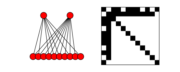
Figure 1: Left: Graphical representation of a latent variable model as an undirected graphical model for a case with somewhat sparse $\mathbf{A}$. Right: The adjacency matrix of the graph showing the sparse pattern of non-zero elements in the corresponding precision matrix.

Let us consider a model for $\mathbf{x}\in\mathbb{R}^{d_{1}},\mathbf{y}\in\mathbb{R}^{d_{2}}$, where $\mathbf{y}=\mathbf{A}\mathbf{x}+\epsilon$. The graphical structure of the model and the corresponding precision matrix structure are illustrated in Fig. 1. Assuming $\mathbf{x}\sim\mathcal{N}(0,\sigma_{x}^{2}I),\epsilon\sim\mathcal{N}(0,\sigma_{\epsilon}^{2}I)$, the covariance of the concatenated vectors $(\mathbf{x}^{T},\mathbf{y}^{T})^{T}$ is given by the block matrix

$$\mathrm{Cov}((\mathbf{x}^{T},\mathbf{y}^{T})^{T})=\mathbf{C}=\sigma_{x}^{2}\begin{pmatrix}I&\mathbf{A}^{T}\\ \mathbf{A}&\mathbf{A}\mathbf{A}^{T}+\sigma_{\epsilon}^{2}I\end{pmatrix}.$$ (4)

The covariance matrix has an analytical block matrix inverse (Lu and Shiou, 2002)

$$\mathbf{C}^{-1}=\sigma_{x}^{-2}\begin{pmatrix}I+\sigma_{\epsilon}^{-2}\mathbf{A}^{T}\mathbf{A}&-\sigma_{\epsilon}^{-2}\mathbf{A}^{T}\\ -\sigma_{\epsilon}^{-2}\mathbf{A}&\sigma_{\epsilon}^{-2}I\end{pmatrix}.$$ (5)

This precision matrix recapitulates the conditional independence result for Gaussian Markov random fields: the lower right block is diagonal because the variables in $\mathbf{y}$ are conditionally independent of each other given $\mathbf{x}$. The matrix is clearly sparse, so we would intuitively assume sparse precision matrix estimation methods should be able to recover it. The non-zero elements do, however, depend on $\sigma_{\epsilon}^{-2}$ which can make them very large if the noise $\sigma_{\epsilon}^{2}$ is small.

It is possible to evaluate and bound the different terms of Eq. (1) evaluated at the ground truth for these models:

$$\log\det(\mathbf{C}^{-1}) =-d_{2}\log\sigma_{\epsilon}^{2}$$

$$-\textnormal{trace}(\mathbf{C}\mathbf{C}^{-1}) =-(d_{1}+d_{2})$$

$$-\lambda||\mathbf{C}^{-1}||_{1} <-\lambda\sigma_{\epsilon}^{-2}(d_{2}+2||\mathbf{A}||_{1}).$$

The magnitude of the last penalty term clearly grows very quickly as $\sigma_{\epsilon}^{2}$ decreases. Clearly the magnitude of the two first log-likelihood terms grows much more slowly as they only depend on $\log\sigma_{\epsilon}^{2}$. Thus the total value of Eq. (1) decreases without bound as $\sigma_{\epsilon}^{2}$ decreases.

Forgetting the ground truth, it is easy to see that one can construct an estimate $\mathbf{\Omega}$ for which the objective remains bounded. If we assume all values of $\mathbf{C}$ to be $\leq 1$ (after normalisation),

$$\textnormal{trace}(\mathbf{C}\mathbf{\Omega})\leq||\mathbf{\Omega}||_{1}.$$

As the other terms only depend on $\mathbf{\Omega}$ it is easy to choose $\mathbf{\Omega}$ so that they remain bounded. The estimate $\mathbf{\Omega}$ that yields these values will in many cases not have anything to do with $\mathbf{C}^{-1}$, as seen in the experiments below.

4 EXPERIMENTS

We tested the performance of glasso, SCIO and CLIME as well as FMPL using the model structure introduced in Sec. 3. The performance of the methods was investigated by varying the noise variance $\sigma_{\epsilon}^{2}$, and the sample size $n$. The model matrix $\mathbf{A}$ was created as a $(d_{2},d_{1})$-array of independent normal random variables with mean $0$ and variance $1$. The majority of the tests were run using input dimensionality $d_{1}=2$, output dimensionality $d_{2}=10$ and noise variance $\sigma_{\epsilon}^{2}=0.1^{2}$ but we also tested varying these settings. For each individual choice of noise and sample size, $k=50$ different matrices $\mathbf{A}$ were generated and the results were averaged.

Generating $n$ samples using model described, data were normalised and analysed using the five different methods. We calibrated the methods in a way that number of edges in the resulting graph would match the true number. Similarly, we thresholded the naive method by taking inverse matrix directly to output the correct number of edges. The FMPL method has no direct tuning parameters so we used its OR mode results as such. Similar tuning is not possible in a real problem where the true number of edges is now known. The tuning represents the best possible results the methods could obtain with an oracle that provides an optimal regularisation parameter.

We evaluated the results using the Hamming distance between the ground truth and the inferred sparsity pattern, i.e. the number of incorrect edges and non-edges which were treated symmetrically. For methods returning the correct number of edges, this value is directly related to the precision $pr$ through

$$d_{\text{Hamming}}=2(1-pr)N_{\text{true positives}}$$

or conversely

$$pr=1-\frac{d_{\text{Hamming}}}{2N_{\text{true positives}}}.$$

We will nevertheless use the Hamming distance as it enables fair comparison with FMPL that sometimes returns a different number of edges.

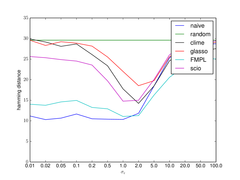
Figure 2: Performances of different methods on latent variable like model with 100 samples. (Lower values are better.)

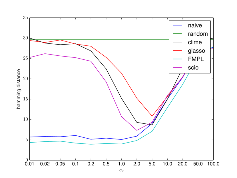
Figure 3: Performances of different methods on latent variable like model with 1000 samples. (Lower values are better.)

Figs. 2 and 3 show the Hamming distance obtained by the different methods as a function of the noise level when using 100 and 1000 samples, respectively. The results show that especially for low but also for high noise levels, the $\ell_{1}$-based methods all perform very poorly with especially glasso and CLIME performing very close to random guessing level for low noise levels $\sigma_{\epsilon}\leq 0.1$. The naive inverse and FMPL work much better up to moderate noise levels of $\sigma_{\epsilon}\approx 2$ after which the noise starts to dominate the signal and the performance of all methods starts to drop. SCIO is a little better than the other $\ell_{1}$-based methods but clearly worse than FMPL and naive in the low noise regime.

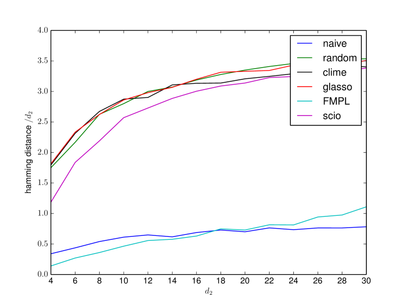
Figure 4: Performances of different methods on latent variable like model with varying output dimensionality. (Lower values are better.)

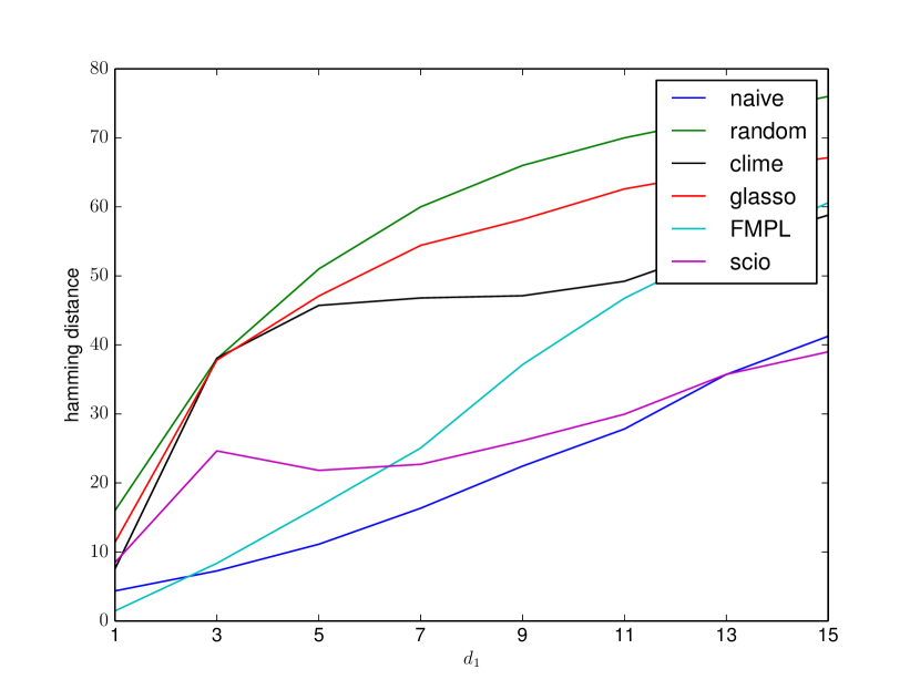
Figure 5: Performances of different methods on latent variable like model with varying input dimensionality. (Lower values are better.)

Fig. 4 shows the results when changing the output dimensionality $d_{2}$ from 10. The results show that the performance of all $\ell_{1}$-based methods is very poor across all $d_{2}$. Glasso performance is close to random guessing level across the entire range considered, while CLIME is slightly better for $d_{2}\geq 18$ and SCIO slightly better across the entire range. Both FMPL and naive are significantly better than any of the $\ell_{1}$-based methods.

Fig. 5 shows the corresponding result when changing the input dimensionality $d_{1}$. The results are now quite different as all methods are better than random especially for larger values. SCIO still outperforms CLIME which outperforms glasso. FMPL is really accurate for small $d_{1}$ but degrades for larger $d_{1}$ while the naive method is the most accurate in almost all cases.

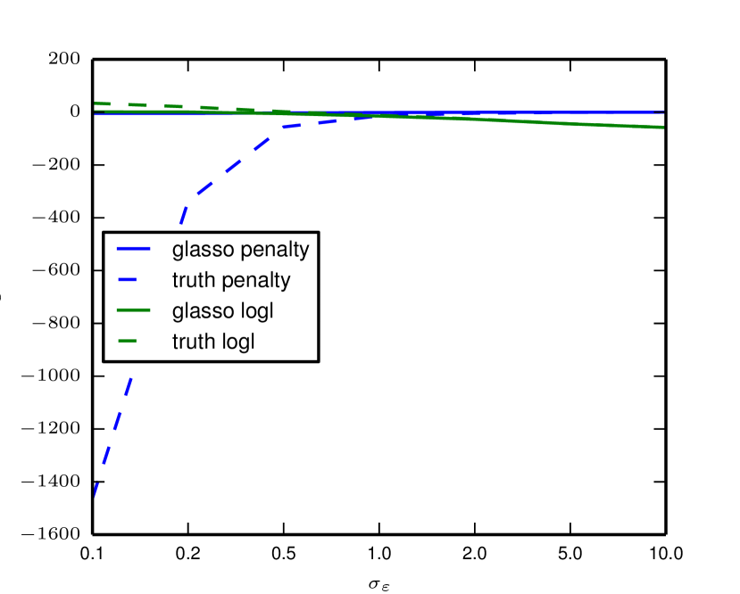
Figure 6: Contributions of the different terms of the glasso objective (1) for latent variable like model with 1000 samples. The green curves show the contributions of the first two terms of Eq. (1) and the blue curves show the contributions of the last penalty term. Solid lines show the result of the glasso optimal solution while dashed lines show the result for the true solution.

To further illustrate the behaviour of glasso on these examples, Fig. 6 shows the contributions of the different parts of the glasso objective function (1) as a function of the noise level both for the true solution (“truth”) as well as the glasso solution. The results show that for low noise levels the penalty incurred by the true solution becomes massive. The glasso solution has a much lower log-likelihood (“logl”) than ground truth but this is amply compensated by the significantly smaller penalty. As the noise increases, the penalty of the true solution decreases and the glasso solution converges to similar values.

4.1 NECESSITY OF ASSUMPTION 1

It can be checked that the norm $\gamma$ in Assumption 1 and Eq. (3) for latent-variable-like models depends on the scale of $\mathbf{A}$. We took advantage of this by creating examples with different values of $\gamma$ and testing the precision of glasso using the true covariance which corresponds to infinite data limit. The results of this experiment are shown in Fig. 7. The results verify that glasso consistently yields perfect results when $\gamma<1$ which is a part of the sufficient conditions for consistency of glasso. As $\gamma$ grows and the sufficient conditions are no longer satisfied, it is clearly seen that the accuracy of glasso starts to deteriorate rapidly. This suggests that the sufficient condition of Assumption 1 is in practice also necessary to ensure consistence.

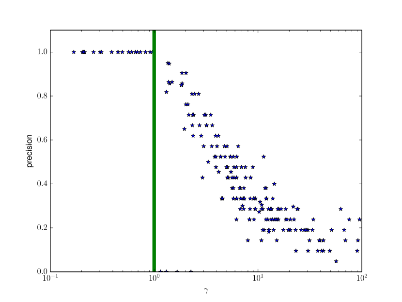
Figure 7: Precision of glasso on infinite data as a function of the norm $\gamma$ of Assumption 1 and Eq. (3). Values to the left of the green vertical line satisfy this condition while values to the right violate it. (Higher values are better.)

5 INCONSISTENCY FOR MODELS OF REAL GENE EXPRESSION DATA

We tested how often the problems presented above appear in real data using the “TCGA breast invasive carcinoma (BRCA) gene expression by RNAseq (IlluminaHiSeq)” data set (Cancer Genome Atlas Network, 2012) downloaded from https://genome-cancer.ucsc.edu/proj/site/hgHeatmap/. The data set contains gene expression measurements for 20530 genes for $n=1215$ samples. After removing genes with a constant expression across all samples there are $p=20252$ genes remaining.

In order to test the methods we randomly sampled subsets of $d$ genes and considered the correlation matrix $\mathbf{C}_{0}$ over that subset. We generated sparse models with known ground truth by computing the corresponding precision matrix $\boldsymbol{\Lambda}_{0}$ from the empirical correlation matrix, setting elements with absolute values below chosen cutoff $\delta=0.1$ to 0 to obtain

$$\boldsymbol{\Lambda}_{ij}=\begin{cases}(\boldsymbol{\Lambda}_{0})_{ij}\quad&\text{if }|(\boldsymbol{\Lambda}_{0})_{ij}|>\delta\\ 0\quad&\text{otherwise}\end{cases}$$ (6)

and the testing covariance matrix $\mathbf{C}=\boldsymbol{\Lambda}^{-1}$. The cutoff lead to networks that were sparse with on average 60% zeros in the precision matrix.

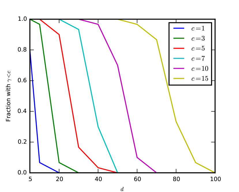
Figure 8: Testing the condition of Assumption 1 of Ravikumar et al. (2011) in Eq. (3) on real gene expression data showing the fraction of random subsets of $d$ genes that fulfil the requirement and various relaxations. The condition (3) requires $\gamma<1$, but the figure shows results also for larger $\gamma$ cutoffs.

Fig. 8 shows the fraction of covariances derived from random subsets of $d$ genes that satisfy the Assumption 1 of Ravikumar et al. (2011) ($c=1$) as well as the fraction of values below more relaxed bounds. The figure shows that the assumption is reliably satisfied only for very small $d$ while for $d\geq 20$, the assumption is essentially never satisfied. Based on the results of Fig. 7 it is likely that glasso results will degrade significantly by for $\gamma>10$ and beyond which are very common for large networks.

We further studied how accurately glasso can recover the graphical structures when the data were generated using the precision matrices described above. We used a similar thresholding with a cut-off value of $0.1$ in order to first form sparse precision matrices for a random subset of genes with given dimension. These matrices were then inverted to obtain covariance matrices. We checked that the resulting matrices were positive definite and then used them to sample multivariate normal data with zero mean with different sample sizes.

The obtained data sets were centred and scaled before computing the sample covariance which was used as input to the glasso algorithm. The regularisation parameter was chosen with the aid of the ground truth graph, so that the the graph identified by glasso would contain as many edges as there were in the real graph. Results are shown in Figure 9. The results show that glasso performance decreases as the network size increases and is approaching that of random guessing for the largest networks considered here.

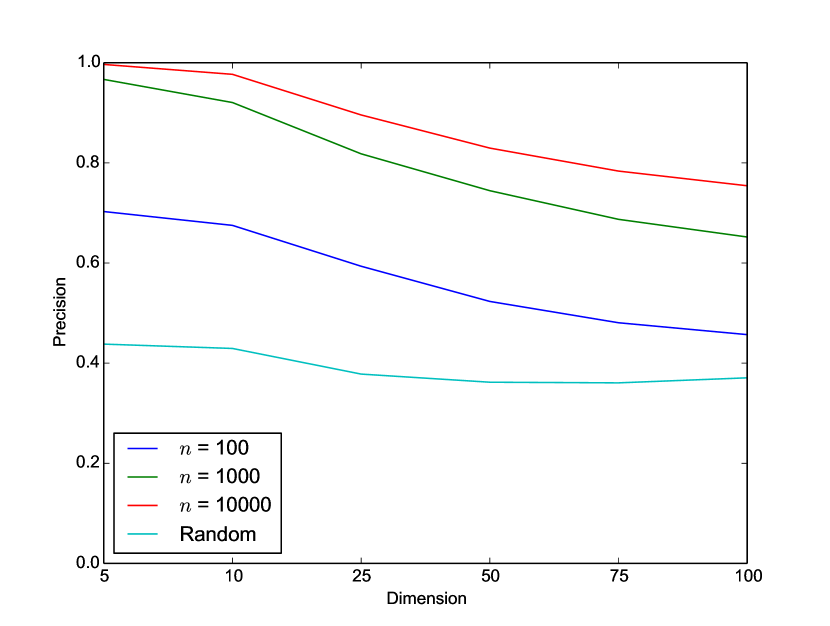
Figure 9: Average precisions for glasso with different dimensions and sample sizes of the real gene expression data, higher values are better. The precision obtained by random guessing is also illustrated.

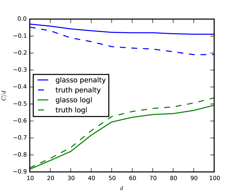
Figure 10: Average contributions of the different terms of the glasso objective function (1) on real gene expression data over random subsets of $d$ genes. The values are shown for the $\ell_{1}$ penalty term as well as the unnormalised log-likelihood, divided by $d$ to make them comparable. Solid lines show the values for glasso result while dashed lines show the result for ground truth.

Fig. 10 shows the contributions of different parts of the glasso objective function (1) as a function of the number of genes $d$. The regularisation parameter $\lambda$ of glasso was tuned to return a solution with the same number of edges as in the true solution. We used the glasso implementation of scikit-learn (Pedregosa et al., 2011), which ignores the diagonal terms of $\boldsymbol{\Omega}$ when computing the penalty. The figure shows clearly how the penalty term for the true solution increases superlinearly as a function of $d$. (A linear increase would correspond to a horizontal line.) The result is even more striking given that the optimal $\lambda$ decreases slightly as $d$ increases. The penalty contribution for glasso solution increases much more slowly. The excess loss in log-likelihood from glasso solution increases as $d$ increases, but this is compensated by a larger saving in the penalty. Together these suggest that glasso solutions are likely to remain further away from ground truth as $d$ increases.

6 DISCUSSION

The class of latent variable like models presented in Sec. 3 is an interesting example of models that have a very clear sparse structure, which all $\ell_{1}$-penalisation-based methods seem unable to recover even in the limit of infinite data. This class complements the previously considered examples of models where glasso is inconsistent including the “two neighbouring triangles” model of Meinshausen (2008) and the star graph of Ravikumar et al. (2011), the latter of which can be seen as a simple special case of our example.

An important question arising from our investigation is how significant the discovered limitation to inferring sparse covariance matrices is in practice, i.e. how common are the latent variable like structures in real data sets. Given the popularity and success of linear models in diverse applications it seems plausible such structures could often exist in real data sets, either as an intrinsic property or as a result of some human intervention, e.g. through inclusion of partly redundant variables.

The gene expression data set is a natural example of an application where graphical model structure learning has been considered. The original glasso paper (Friedman et al., 2008) contained an example on learning gene networks, although from proteomics data. Other authors (e.g. Ma et al., 2007) have applied Gaussian graphical models and even glasso (e.g. Menéndez et al., 2010) to gene network inference from expression data. Our experiments on the TCGA gene expression data suggest that in such applications it is advisable to consider the conditions for the consistency of $\ell_{1}$ penalised methods very carefully when planning to apply those.

Previous publications presenting new methods for sparse precision matrix have typically tested the method on synthetic examples where the true precision matrix is specified to contain mostly small values. Specifying the precision matrix provides a convenient way to generate test cases as the sparsity pattern can be defined very naturally through it. At the same time, this excludes any models that have an ill-conditioned covariance. As shown by our example, such ill-conditioned covariances arise very naturally from model structures that are plausible from the application perspective.

Ultimately, our results suggest that users of the numerous $\ell_{1}$ penalised methods should be much more careful about checking whether the conditions of consistency for precision matrix estimation are likely to be fulfilled in the application area of interest.

Acknowledgements

This work was supported by the Academy of Finland [259440 to A.H., 251170 to J.C.] and the European Research Council [239784 to J.C.].

References

- Banerjee et al. (2008) O. Banerjee, L. El Ghaoui, and A. d’Aspremont. Model selection through sparse maximum likelihood estimation for multivariate Gaussian or binary data. Journal of Machine Learning Research, 9:485–516, June 2008.
- Cai et al. (2011) T. Cai, W. Liu, and X. Luo. A constrained minimization approach to sparse precision matrix estimation. Journal of the American Statistical Association, 106(494):594–607, Jun 2011.
- Cancer Genome Atlas Network (2012) Cancer Genome Atlas Network. Comprehensive molecular portraits of human breast tumours. Nature, 490(7418):61–70, Oct 2012.
- Friedman et al. (2008) J. Friedman, T. Hastie, and R. Tibshirani. Sparse inverse covariance estimation with the graphical lasso. Biostatistics, 9(3):432–441, Jul 2008.
- Hsieh et al. (2014) C. Hsieh, M. A. Sustik, I. S. Dhillon, and P. D. Ravikumar. QUIC: quadratic approximation for sparse inverse covariance estimation. Journal of Machine Learning Research, 15(1):2911–2947, 2014.
- Lauritzen (1996) S. Lauritzen. Graphical Models. Clarendon Press, 1996. ISBN 9780191591228.
- Leppä-aho et al. (2016) J. Leppä-aho, J. Pensar, T. Roos, and J. Corander. Learning Gaussian graphical models with fractional marginal pseudo-likelihood. arXiv:1602.07863, 2016.
- Liu and Luo (2015) W. Liu and X. Luo. Fast and adaptive sparse precision matrix estimation in high dimensions. Journal of Multivariate Analysis, 135:153 – 162, 2015.
- Lu and Shiou (2002) T.-T. Lu and S.-H. Shiou. Inverses of block matrices. Computers & Mathematics with Applications, 43(1-2):119–129, Jan 2002.
- Ma et al. (2007) S. Ma, Q. Gong, and H. J. Bohnert. An Arabidopsis gene network based on the graphical Gaussian model. Genome Res, 17(11):1614–1625, Nov 2007.
- Meinshausen (2008) N. Meinshausen. A note on the Lasso for Gaussian graphical model selection. Statistics & Probability Letters, 78(7):880–884, May 2008.
- Meinshausen and Bühlmann (2006) N. Meinshausen and P. Bühlmann. High-dimensional graphs and variable selection with the lasso. The Annals of Statistics, 34(3):1436–1462, Jun 2006.
- Menéndez et al. (2010) P. Menéndez, Y. A. I. Kourmpetis, C. J. F. ter Braak, and F. A. van Eeuwijk. Gene regulatory networks from multifactorial perturbations using Graphical Lasso: application to the DREAM4 challenge. PLoS One, 5(12):e14147, 2010.
- Pedregosa et al. (2011) F. Pedregosa, G. Varoquaux, A. Gramfort, V. Michel, B. Thirion, O. Grisel, M. Blondel, P. Prettenhofer, R. Weiss, V. Dubourg, J. Vanderplas, A. Passos, D. Cournapeau, M. Brucher, M. Perrot, and E. Duchesnay. Scikit-learn: Machine learning in Python. Journal of Machine Learning Research, 12:2825–2830, 2011.
- Peng et al. (2009) J. Peng, P. Wang, N. Zhou, and J. Zhu. Partial correlation estimation by joint sparse regression models. Journal of the American Statistical Association, 104(486):735–746, 2009.
- Ravikumar et al. (2011) P. Ravikumar, M. J. Wainwright, G. Raskutti, and B. Yu. High-dimensional covariance estimation by minimizing -penalized log-determinant divergence. Electronic Journal of Statistics, 5:935–980, 2011.
- Tibshirani (1996) R. Tibshirani. Regression shrinkage and selection via the lasso. Journal of the Royal Statistical Society, Series B, 58:267–288, 1996.
- Whittaker (1990) J. Whittaker. Graphical Models in Applied Multivariate Statistics. John Wiley & Sons, 1990.
- Yuan and Lin (2007) M. Yuan and Y. Lin. Model selection and estimation in the Gaussian graphical model. Biometrika, 94(1):19–35, 2007.
- Zhao and Yu (2006) P. Zhao and B. Yu. On model selection consistency of lasso. Journal of Machine Learning Research, 7:2541–2563, 2006.