Nested sampling, statistical physics and the Potts model

Manuel J. Pfeifenberger Erich Schmid Institute of Materials Science, Austrian Academy of Sciences, 8700 Leoben, Austria manuel.pfeifenberger@oeaw.ac.at Michael Rumetshofer Wolfgang von der Linden Institute of Theoretical and Computational Physics, Graz University of Technology, 8010 Graz, Austria
Abstract

We present a systematic study of the nested sampling algorithm based on the example of the Potts model. This model, which exhibits a first order phase transition for q>4๐‘ž4q>4, exemplifies a generic numerical challenge in statistical physics: The evaluation of the partition function and thermodynamic observables, which involve high dimensional sums of sharply structured multi-modal density functions. It poses a major challenge to most standard numerical techniques, such as Markov Chain Monte Carlo. In this paper we will demonstrate that nested sampling is particularly suited for such problems and it has a couple of advantages. For calculating the partition function of the Potts model with N๐‘N sites: a) one run stops after Oโ€‹(N)๐‘‚๐‘O(N) moves, so it takes Oโ€‹(N2)๐‘‚superscript๐‘2O(N^{2}) operations for the run, b) only a single run is required to compute the partition function along with the assignment of confidence intervals, c) the confidence intervals of the logarithmic partition function decrease with 1/N1๐‘1/\sqrt{N} and d) a single run allows to compute quantities for all temperatures while the autocorrelation time is very small, irrespective of temperature. Thermodynamic expectation values of observables, which are completely determined by the bond configuration in the representation of Fortuin and Kasteleyn, like the Helmholtz free energy, the internal energy as well as the entropy and heat capacity, can be calculated in the same single run needed for the partition function along with their confidence intervals. In contrast, thermodynamic expectation values of magnetic properties like the magnetization and the magnetic susceptibility require sampling the additional spin degree of freedom. Results and performance are studied in detail and compared with those obtained with multi-canonical sampling. Eventually the implications of the findings on a parallel implementation of nested sampling are outlined.

keywords:
Nested sampling , Potts model , Magnetic susceptibility , Parallel nested sampling , Partition function , Statistical physics

1 Introduction

Monte Carlo (MC) simulations are the most important instrument for the evaluation of integrals or sums in a high dimensional phase space. When it comes to the computation of partition functions there are only very few reliable techniques, such as simulated tempering [1], multi-canonical sampling (MUCA) [2, 3], or multi-bondic cluster algorithms (MUBO) [4] available that guarantee perfect mixing. Skilling, however, gave an example, where also MUCA would fail [5]. Basically, these algorithms are trying to enhance the efficiency of the MC algorithm by flattening the probability distribution. A conceptual completely different approach, named nested sampling (NESA), has been suggested by Skilling [5]. It is a promising way for estimating high dimensional, multi-modal integrals or sums and is based on a mapping to a Lebesgue integral along with a novel sampling technique. Since its development it has already found its way into various fields of research. Especially in statistics and Bayesian inference various applications already exist [6, 7, 8, 9, 10]. Furthermore, for atomistic modelling and materials simulations NESA has proven to be an highly efficient algorithm [11, 12, 13]. A first, though incomplete, application in the field of statistical physics, in particular for the Potts model, has been presented by Murray et al.[14]. The Potts model provides, despite of its simple structure, a wide variety of interesting physical properties and the availability of exact results for certain quantities of the two dimensional model makes it an optimal playground for testing new approaches in simulation techniques. For parameters, where the model exhibits a first order phase transition, the numerical evaluation of the partition function poses a severe difficulty for standard MC algorithms, because at first order phase transitions the autocorrelation times can become huge. Moreover, such systems are characterized by a double-peak structure in the probability density for the energy with a pronounced minimum in between, which is exponentially suppressed due to the interface tension. This causes severe mixing problems in standard Monte Carlo techniques [15]. In this case two or more well separated phase space regions need to be explored. Transitions between these regions are possible but very improbable and therefore the relative weights of the maxima will not be sampled correctly. Multi-canonical sampling (MUCA) and multi-bondic sampling (MUBO) are particularly tailored to overcome this barrier [2, 3, 4]. A detailed analysis and comparison is given by Janke [16].

In the present work the implementation of nested sampling for evaluating the partition function and thermodynamic expectation values of the Potts model and its accuracy are significantly improved as compared to that in [14] and in particular, no additional thermodynamic integration is required. We compute thermodynamic expectation values like the internal energy, the entropy, the magnetization and the magnetic susceptibility along with confidence intervals applying NESA, discuss the results and compare to MUCA, theoretical values and limiting cases. Moreover, the performance of NESA is thoroughly investigated and compared with the performance of MUCA. Already in his original paper [5] Skilling mentioned the possibility of a faster exploration of the phase space via a parallel implementation of nested sampling. This idea has recently been picked up in various publications ([7, 17, 18, 19]). In this paper we will explore the capability of parallel nested sampling.

The paper is organized as follows: In Sec. 2 the Potts model is introduced. The MC methods employed by us to compute the partition function of the Potts model, namely multi-canonical simulation and nested sampling are described in Sec. 3.1 and Sec. 3.2, respectively. Being in the focus of our investigation, NESA is treated in a more elaborate way. Results for the Potts model are compiled in Sec. 4. A performance comparison of NESA and MUCA is shown in Sec. 4.8. Furthermore, it is presented how thermodynamic variables can be evaluated from a single nested sampling run. Consequences for a parallel implementation are discussed in Sec. 4.9. Finally the results are discussed and potential generalizations are outlined.

2 Potts model

One of the most investigated models in statistical physics is the Potts model [20]. The corresponding Hamiltonian, without external fields, reads

Hโ€‹(๐ฌ)๐ป๐ฌ\displaystyle H(\mathbf{s}) =โˆ’Jโ€‹โˆ‘โŸจi,jโŸฉ(ฮดsi,sjโˆ’1)=โˆ’Jโ€‹(Neqโ€‹(๐ฌ)โˆ’Np).absent๐ฝsubscript๐‘–๐‘—subscript๐›ฟsubscript๐‘ ๐‘–subscript๐‘ ๐‘—1๐ฝsubscript๐‘eq๐ฌsubscript๐‘p\displaystyle=-J\>\sum_{\left\langle i,j\right\rangle}\big{(}\delta_{s_{i},s_{j}}-1\big{)}=-J\big{(}N_{\text{eq}}(\mathbf{s})-N_{\text{p}}\big{)}\;. (1)

The dynamic variables sisubscript๐‘ ๐‘–s_{i} of the model, referred to as spin or color, can assume the integer values between 1 and q๐‘žq. The term Neqโ€‹(๐ฌ)=โˆ‘โŸจi,jโŸฉฮดsi,sjsubscript๐‘eq๐ฌsubscript๐‘–๐‘—subscript๐›ฟsubscript๐‘ ๐‘–subscript๐‘ ๐‘—N_{\text{eq}}(\mathbf{s})=\sum_{\left\langle i,j\right\rangle}\delta_{s_{i},s_{j}} is the number of nearest neighbour pairs with equal spin, and Npsubscript๐‘pN_{\text{p}} is the total number of nearest neighbour pairs in the lattice under consideration. Here the exchange coupling J๐ฝJ is positive and site independent. The lattice indices are denoted by i๐‘–i and j๐‘—j, ranging from 1 to the number of sites N๐‘N. The sum only includes nearest neighbour interactions which is denoted by โŸจi,jโŸฉ๐‘–๐‘—\left\langle i,j\right\rangle. The sought-for partition function reads

ZPโ€‹(๐•“)subscript๐‘P๐•“\displaystyle Z_{\text{P}}(\mathbbm{b}) =โˆ‘๐ฌe๐•“โ€‹โˆ‘โŸจi,jโŸฉ(ฮดsi,sjโˆ’1),absentsubscript๐ฌsuperscript๐‘’๐•“subscript๐‘–๐‘—subscript๐›ฟsubscript๐‘ ๐‘–subscript๐‘ ๐‘—1\displaystyle=\sum_{\mathbf{s}}e^{\mathbbm{b}\>\sum_{\left\langle i,j\right\rangle}\big{(}\delta_{s_{i},s_{j}}-1\big{)}}\;, (2)

with the abbreviation ๐•“=ฮฒโ€‹J๐•“๐›ฝ๐ฝ\mathbbm{b}=\beta J. Two limiting cases can easily be determined

Zโ€‹(๐•“)๐‘๐•“\displaystyle Z(\mathbbm{b}) โŸถ๐•“โ†’0โ€‹qN,Zโ€‹(๐•“)โ€‹โŸถ๐•“โ†’โˆžโ€‹q,โ†’๐•“0โŸถsuperscript๐‘ž๐‘๐‘๐•“โ†’๐•“โŸถ๐‘ž\displaystyle\underset{\mathbbm{b}\to 0}{\longrightarrow}q^{N}\;,\qquad Z(\mathbbm{b})\underset{\mathbbm{b}\to\infty}{\longrightarrow}q\;, (3)

which will be of interest later on. In the first case (high temperature limit), the Boltzmann factor is one for all spin configurations while in the second (low temperature limit) only those configurations contribute, where all spins have the same value. Our investigations are restricted to 2d square lattices with periodic boundary conditions. The infinite square lattice exhibits for qโ‰ค4๐‘ž4q\leq 4 (q>4๐‘ž4q>4) a second (first) order phase transition. The exact critical inverse temperature for the Potts model on a two dimensional infinite square lattice follows from self-duality of the low and high temperature region [21]

๐•“c=lnโก(1+q).subscript๐•“๐‘1๐‘ž\displaystyle\mathbbm{b}_{c}=\ln(1+\sqrt{q}). (4)

3 Evaluation of the partition function

Quite generally, the partition function Z๐‘Z, associated to the thermodynamic potential (Helmholtz free energy), contains the entire thermodynamic information of a system in the canonical ensemble. It can be expressed as

Z=โˆ‘โˆซ๐ฑโกLโ€‹(๐ฑ)โ€‹ฯ€โ€‹(๐ฑ),๐‘subscript๐ฑ๐ฟ๐ฑ๐œ‹๐ฑ\displaystyle Z=\operatorname*{\mathchoice{\ooalign{$\displaystyle\sum$\cr$\displaystyle\int$\cr}}{\ooalign{\raisebox{0.14pt}{\scalebox{0.7}{$\textstyle\sum$}}\cr$\textstyle\int$\cr}}{\ooalign{\raisebox{0.2pt}{\scalebox{0.6}{$\scriptstyle\sum$}}\cr$\scriptstyle\int$\cr}}{\ooalign{\raisebox{0.2pt}{\scalebox{0.6}{$\scriptstyle\sum$}}\cr$\scriptstyle\int$\cr}}}\limits_{\mathbf{x}}\>L(\mathbf{x})\>\pi(\mathbf{x}), (13)

where ๐ฑ๐ฑ\mathbf{x} describes a point in a multidimensional phase space, which can either be continuous or discrete. In the following Lโ€‹(๐ฑ)๐ฟ๐ฑL(\mathbf{x}) is denoted as likelihood function and ฯ€โ€‹(๐ฑ)๐œ‹๐ฑ\pi(\mathbf{x}) as prior probability. Assuming the likelihood function Lโ€‹(๐ฑ)๐ฟ๐ฑL(\mathbf{x}) shows a strong variation, then a classical Markov Chain MC needs a huge sample size to yield reasonable variances [22]. For the evaluation of Z special methods exist. Two of them will be presented in the following subsections.

3.1 Multi-canonical simulation and the partition function

Multi-canonical simulation (MUCA) is a method introduced by Berg and Neuhaus [23, 24] and thoroughly investigated by Janke [25, 15]. The underlying idea is briefly as follows. We start out from the Boltzmann distribution

pcanโ€‹(๐ฑ)=1Zโ€‹eโˆ’๐•“โ€‹Eโ€‹(๐ฑ),subscript๐‘can๐ฑ1๐‘superscript๐‘’๐•“๐ธ๐ฑ\displaystyle p_{\text{can}}(\mathbf{x})=\frac{1}{Z}e^{-\mathbbm{b}E(\mathbf{x})}\;, (14)

where energies are measured in units of J๐ฝJ. For the multi-canonical probability distribution an additional weight function wโ€‹(E):=eโˆ’gโ€‹(E)assign๐‘ค๐ธsuperscript๐‘’๐‘”๐ธw(E):=e^{-g(E)} is introduced that defines a new probability distribution

pmucaโ€‹(๐ฑ)=pcanโ€‹(๐ฑ)โ€‹wโ€‹(Eโ€‹(๐ฑ)),subscript๐‘muca๐ฑsubscript๐‘can๐ฑ๐‘ค๐ธ๐ฑ\displaystyle p_{\text{muca}}(\mathbf{x})=p_{\text{can}}(\mathbf{x})w(E(\mathbf{x})), (15)

which is used in the MC simulation. The goal of MUCA is to choose the additional weights such that the resulting density of energy states is almost flat, i.e.

โˆ‘๐’™wโ€‹(Eโ€‹(๐’™))โ€‹ฮดโ€‹(Eโˆ’Eโ€‹(๐’™))subscript๐’™๐‘ค๐ธ๐’™๐›ฟ๐ธ๐ธ๐’™\displaystyle\sum_{\boldsymbol{x}}w(E(\boldsymbol{x}))\delta(E-E(\boldsymbol{x})) โ‰ˆconst,absentconst\displaystyle\approx\text{const}\;, (16)

within a relevant energy window. In other words, the inverse of wโ€‹(E)๐‘ค๐ธw(E) is a rough approximation of the density of states ฯโ€‹(E)๐œŒ๐ธ\rho(E). This guarantees better mixing for systems with pronounced multi-modal structures. In principle, a flat density can also be strived for other parameters, e.g. magnetization. The weight wโ€‹(Eโ€‹(๐ฑ))๐‘ค๐ธ๐ฑw(E(\mathbf{x})) is not known in the beginning, otherwise we would already know ฯโ€‹(E)๐œŒ๐ธ\rho(E) and a direct evaluation of Z๐‘Z as sum over energies would be an easy task. It is generally iteratively determined by repeated simulations. More details can be found in [25, 2, 3]. Apart from a yet unknown normalization constant Zwsubscript๐‘๐‘คZ_{w}, we define a new probability density function (PDF) for a configuration ๐ฑ๐ฑ\mathbf{x} as p(0)โ€‹(๐ฑ)=wโ€‹(Eโ€‹(๐ฑ))/Zwsuperscript๐‘0๐ฑ๐‘ค๐ธ๐ฑsubscript๐‘๐‘คp^{(0)}(\mathbf{x})=w(E(\mathbf{x}))/Z_{w}. The partition function can then be expressed as

Z๐•“subscript๐‘๐•“\displaystyle Z_{\mathbbm{b}} =Zwโ€‹โˆ‘๐ฑeโˆ’๐•“โ€‹Eโ€‹(๐ฑ)+gโ€‹(Eโ€‹(๐ฑ))โ€‹p(0)โ€‹(Eโ€‹(๐ฑ)).absentsubscript๐‘๐‘คsubscript๐ฑsuperscript๐‘’๐•“๐ธ๐ฑ๐‘”๐ธ๐ฑsuperscript๐‘0๐ธ๐ฑ\displaystyle=Z_{w}\sum_{\mathbf{x}}\;{e^{-\mathbbm{b}E(\mathbf{x})+g(E(\mathbf{x}))}\;p^{(0)}(E(\mathbf{x}))}\;. (17)

MUCA uses p(0)superscript๐‘0p^{(0)} to guide the random walk and it yields a sample of configurations ๐ฑ๐ฑ\mathbf{x} of size L๐ฟL, say. We can then estimate the partition function by

Z๐•“subscript๐‘๐•“\displaystyle Z_{\mathbbm{b}} =ZwLโ€‹โˆ‘n=1Leโˆ’๐•“โ€‹Eโ€‹(๐ฑn)+gโ€‹(Eโ€‹(๐ฑn))=Zwโ€‹โˆ‘Eeโˆ’๐•“โ€‹E+gโ€‹(E)โ€‹hโ€‹(E),absentsubscript๐‘๐‘ค๐ฟsuperscriptsubscript๐‘›1๐ฟsuperscript๐‘’๐•“๐ธsubscript๐ฑ๐‘›๐‘”๐ธsubscript๐ฑ๐‘›subscript๐‘๐‘คsubscript๐ธsuperscript๐‘’๐•“๐ธ๐‘”๐ธโ„Ž๐ธ\displaystyle=\frac{Z_{w}}{L}\sum_{n=1}^{L}\;e^{-\mathbbm{b}E(\mathbf{x}_{n})+g(E(\mathbf{x}_{n}))}=Z_{w}\sum_{E}\;e^{-\mathbbm{b}E+g(E)}\;h(E)\;, (18)

where hโ€‹(E)โ„Ž๐ธh(E) is the relative frequency of the occurrence of energy E๐ธE in the Markov chain. Similarly for the internal energy we obtain

U๐•“MUCAsubscriptsuperscript๐‘ˆMUCA๐•“\displaystyle U^{\text{MUCA}}_{\mathbbm{b}} =โˆ‘EEโ€‹eโˆ’๐•“โ€‹E+gโ€‹(E)โ€‹hโ€‹(E)โˆ‘Eeโˆ’๐•“โ€‹E+gโ€‹(E)โ€‹hโ€‹(E).absentsubscript๐ธ๐ธsuperscript๐‘’๐•“๐ธ๐‘”๐ธโ„Ž๐ธsubscript๐ธsuperscript๐‘’๐•“๐ธ๐‘”๐ธโ„Ž๐ธ\displaystyle=\frac{\sum_{E}\;E\;e^{-\mathbbm{b}E+g(E)}\;h(E)}{\sum_{E}\;e^{-\mathbbm{b}E+g(E)}\;h(E)}\;. (19)

For the partition function we still need the normalization Zwsubscript๐‘๐‘คZ_{w}. It can be determined via the exact limiting case ๐•“=0๐•“0\mathbbm{b}=0, or ๐•“โ†’โˆžโ†’๐•“\mathbbm{b}\to\infty. To this end we consider

Z๐•“Z๐•“โ€ฒsubscript๐‘๐•“subscript๐‘superscript๐•“โ€ฒ\displaystyle\frac{Z_{\mathbbm{b}}}{Z_{\mathbbm{b}^{\prime}}} =โˆ‘Eeโˆ’๐•“โ€‹E+gโ€‹(E)โ€‹p(0)โ€‹(E)โˆ‘Eeโˆ’๐•“โ€ฒโ€‹E+gโ€‹(E)โ€‹p(0)โ€‹(E).absentsubscript๐ธsuperscript๐‘’๐•“๐ธ๐‘”๐ธsuperscript๐‘0๐ธsubscript๐ธsuperscript๐‘’superscript๐•“โ€ฒ๐ธ๐‘”๐ธsuperscript๐‘0๐ธ\displaystyle=\frac{\sum_{E}e^{-\mathbbm{b}E+g(E)}p^{(0)}(E)}{\sum_{E}e^{-\mathbbm{b}^{\prime}E+g(E)}p^{(0)}(E)}\;. (20)

For the two limiting cases we have according to Eq.โ€‰(3) Z๐•“=0=qNsubscript๐‘๐•“0superscript๐‘ž๐‘Z_{\mathbbm{b}=0}=q^{N} and Z๐•“โ†’โˆž=qsubscript๐‘โ†’๐•“๐‘žZ_{\mathbbm{b}\to\infty}=q and the MUCA estimate yields

Z๐•“subscript๐‘๐•“\displaystyle Z_{\mathbbm{b}} =qNโ€‹โˆ‘Eeโˆ’๐•“โ€‹E+gโ€‹(E)โ€‹hโ€‹(E)โˆ‘Eegโ€‹(E)โ€‹hโ€‹(E)absentsuperscript๐‘ž๐‘subscript๐ธsuperscript๐‘’๐•“๐ธ๐‘”๐ธโ„Ž๐ธsubscript๐ธsuperscript๐‘’๐‘”๐ธโ„Ž๐ธ\displaystyle=q^{N}\;\frac{\sum_{E}e^{-\mathbbm{b}E+g(E)}h(E)}{\sum_{E}e^{g(E)}h(E)}\; (high temperature limit)high temperature limit\displaystyle(\text{\it high temperature limit}) (21a)
Z๐•“subscript๐‘๐•“\displaystyle Z_{\mathbbm{b}} =qโ€‹โˆ‘Eeโˆ’๐•“โ€‹(Eโˆ’E0)+gโ€‹(E)โ€‹hโ€‹(E)egโ€‹(E0)โ€‹hโ€‹(E0)absent๐‘žsubscript๐ธsuperscript๐‘’๐•“๐ธsubscript๐ธ0๐‘”๐ธโ„Ž๐ธsuperscript๐‘’๐‘”subscript๐ธ0โ„Žsubscript๐ธ0\displaystyle=q\;\frac{\sum_{E}e^{-\mathbbm{b}(E-E_{0})+g(E)}h(E)}{e^{g(E_{0})}h(E_{0})}\; (low temperature limit),low temperature limit\displaystyle(\text{\it low temperature limit})\;, (21b)

where E0subscript๐ธ0E_{0} is the lowest energy of the model.

3.2 Nested sampling

The goal is again the numerical evaluation of the partition function in Eq.โ€‰(13) Later on we will present adequate terms for likelihood and prior in case of the Potts model. Skilling [5] proposed to express Z๐‘Z as Lebesgue integral

Z=โˆซXโ€‹(L)โ€‹๐‘‘L,๐‘๐‘‹๐ฟdifferential-d๐ฟ\displaystyle Z=\int\>X(L)\,dL\;, (22)

where the integral runs over the likelihood values L๐ฟL and Xโ€‹(L)๐‘‹๐ฟX(L) stands for the prior mass

Xโ€‹(L)๐‘‹๐ฟ\displaystyle X(L) =โˆ‘โˆซxโกฯ€โ€‹(๐’™)โ€‹ฮธโ€‹(Lโ€‹(๐’™)>L).absentsubscript๐‘ฅ๐œ‹๐’™๐œƒ๐ฟ๐’™๐ฟ\displaystyle=\operatorname*{\mathchoice{\ooalign{$\displaystyle\sum$\cr$\displaystyle\int$\cr}}{\ooalign{\raisebox{0.14pt}{\scalebox{0.7}{$\textstyle\sum$}}\cr$\textstyle\int$\cr}}{\ooalign{\raisebox{0.2pt}{\scalebox{0.6}{$\scriptstyle\sum$}}\cr$\scriptstyle\int$\cr}}{\ooalign{\raisebox{0.2pt}{\scalebox{0.6}{$\scriptstyle\sum$}}\cr$\scriptstyle\int$\cr}}}\limits_{x}\;\pi(\boldsymbol{x})\;\theta\big{(}L(\boldsymbol{x})>L\big{)}\;. (31)

Equivalently, the partition function can then be expressed as

Z=โˆซ01๐‘‘Xโ€‹โ„’โ€‹(X).๐‘superscriptsubscript01differential-d๐‘‹โ„’๐‘‹\displaystyle Z=\int_{0}^{1}\>dX\,{\cal L}(X)\;. (32)

The derivation of the last three equations can be found in the appendix 6.1. Some minor modifications in the derivation are due in the case of a discrete configuration space. They are outlined in section 6.2. Additional information can be found in [26]. Finally, the integral in Eq.โ€‰(22) is approximated by a Riemann sum

Z=โˆ‘n=0โˆžโ„’(Xn)ฮ”Xn,ฮ”Xn=Xnโˆ’Xn+1.\displaystyle Z=\sum_{n=0}^{\infty}\>{\cal L}(X_{n})\Delta X_{n}\quad,\quad\Delta X_{n}=X_{n}-X_{n+1}\;. (33)

Because the likelihood is a monotonically decreasing function of the prior mass, Eq.โ€‰(33) represents a lower bound of the integral. Replacing โ„’โ€‹(Xn)โ„’subscript๐‘‹๐‘›{\cal L}(X_{n}) by โ„’โ€‹(Xn+1)โ„’subscript๐‘‹๐‘›1{\cal L}(X_{n+1}) yields an upper bound. It is needless to say that the computation of โ„’โ€‹(X)โ„’๐‘‹{\cal L}(X) is as complicated as the original evaluation of Z๐‘Z, but due to Skilling [5], an algorithm can be constructed that avoids the actual knowledge of โ„’โ€‹(X)โ„’๐‘‹{\cal L}(X). The pseudo code is given in 3.2.

{pseudocode}

[ruled]NESA algorithm{ฮป^*_n},n_max input parameters: K,k,ฯต_ฮป

initialize ฮป^*_0=0,โ€… n=0,

draw K configurationsโ€… {x_i}โ€… at random from ฯ€(xโ€‰โ€”โ€‰ฮป^*_0)

sort likelihood values ฮปi=โ„’โ€‹(xi)subscript๐œ†๐‘–โ„’subscript๐‘ฅ๐‘–\lambda_{i}={\cal L}(x_{i}) in increasing order

determine the kthsuperscript๐‘˜thk^{\text{th}} smallest likelihood, denoted by ฮป^*

set ฮป^*_n=1:= ฮป^*

\WHILE

ฮป^*_n+1-ฮป^*_n โ€… ยฟ โ€… ฯต_ฮป \DO\BEGINn \GETSn+1

discard configurations with ฮป_iโ‰คฮป^*_n

replace them by new configurations as follows:

parallel\BEGINstart thread j=1,2,โ€ฆ,k๐‘—12โ€ฆ๐‘˜j=1,2,...,k

draw โ€… x_n^jโ€… from ฯ€(xโ€‰โ€”โ€‰ฮป^*_n)

\END

determine the kthsuperscript๐‘˜thk^{\text{th}} smallest likelihood ฮปโˆ—superscript๐œ†\lambda^{*} of all walkers

set ฮป^*_n+1=ฮป^* \END

set nmax=nsubscript๐‘›max๐‘›n_{\text{max}}=n

\RETURN

{ ฮป^*_n},n_max

In the initialization it is assumed that likelihood values are not negative (hence ฮป0โˆ—=0subscriptsuperscript๐œ†00\lambda^{*}_{0}=0), which will be the case for the Potts model. During the NESA simulation K๐พK configurations ๐ฑ๐ฑ\mathbf{x} (walkers) are treated simultaneously. In each step k๐‘˜k of the walkers, those with the smallest likelihood values, are replaced by new configurations, drawn from the prior subject to the constraint Lโ€‹(๐ฑ)>ฮปnโˆ—๐ฟ๐ฑsubscriptsuperscript๐œ†๐‘›L(\mathbf{\boldsymbol{x}})>\lambda^{*}_{n}. The replacement of k๐‘˜k walkers is ideally suited for parallelization (see Sec. 4.9). The nested sampling moves in configuration space ensure that even well separated peaks of the likelihood function in configuration space are sampled correctly (see [26]). The crucial step for the nested sampling algorithm is to draw from the constrained prior probability

ฯ€โ€‹(๐ฑ|ฮปnโˆ’1โˆ—)=ฯ€โ€‹(๐ฑ)Xโ€‹(ฮปnโˆ’1โˆ—)โ€‹ฮ˜โ€‹(Lโ€‹(๐ฑ)>ฮปnโˆ’1โˆ—),๐œ‹conditional๐ฑsubscriptsuperscript๐œ†๐‘›1๐œ‹๐ฑ๐‘‹subscriptsuperscript๐œ†๐‘›1ฮ˜๐ฟ๐ฑsubscriptsuperscript๐œ†๐‘›1\displaystyle\pi(\mathbf{x}\,\boldsymbol{|}\,\lambda^{*}_{n-1})=\frac{\pi(\mathbf{x})}{X(\lambda^{*}_{n-1})}\>\Theta(L(\mathbf{x})\>>\>\lambda^{*}_{n-1})\;, (34)

which represents the normalized prior restricted to areas, where Lโ€‹(๐ฑ)๐ฟ๐ฑL(\mathbf{x}) exceeds the ฮป๐œ†\lambda threshold. There exist various ways to draw random configurations from this prior. In the approach employed here, new walkers are determined by choosing k๐‘˜k of the remaining Kโˆ’k๐พ๐‘˜K-k walkers at random, since they already represent a valid sample of the constraint prior, and to modify them by suitabel MC steps. Given the likelihood minima ฮปnโˆ—subscriptsuperscript๐œ†๐‘›\lambda^{*}_{n}, the Riemann sum in Eq.โ€‰(33) is estimated by

ZNESA=โˆ‘n=1โˆžฮปnโˆ—โ€‹ฮ”โ€‹Xn.subscript๐‘NESAsuperscriptsubscript๐‘›1subscriptsuperscript๐œ†๐‘›ฮ”subscript๐‘‹๐‘›\displaystyle Z_{\text{NESA}}=\sum_{n=1}^{\infty}\>\lambda^{*}_{n}\Delta{X}_{n}. (35)

We assume that the likelihood has an upper limit ฮปmax=max๐’™โกLโ€‹(๐’™)subscript๐œ†maxsubscript๐’™๐ฟ๐’™\lambda_{\text{max}}=\max_{\boldsymbol{x}}L(\boldsymbol{x}), which will be the case for the Potts model, and which will be reached at step n=nmax๐‘›subscript๐‘›maxn=n_{\text{max}}. Then we can stop the nested sampling run and proceed as follows

ZNESAsubscript๐‘NESA\displaystyle Z_{\text{NESA}} =โˆ‘n=0nmaxโˆ’1ฮปnโˆ—โ€‹ฮ”โ€‹XnโŸ=ZNESA1+ฮปmaxโˆ—โ€‹โˆ‘n=nmaxโˆžฮ”โ€‹Xn.absentsubscriptโŸsuperscriptsubscript๐‘›0subscript๐‘›max1subscriptsuperscript๐œ†๐‘›ฮ”subscript๐‘‹๐‘›absentsuperscriptsubscript๐‘NESA1subscriptsuperscript๐œ†maxsuperscriptsubscript๐‘›subscript๐‘›maxฮ”subscript๐‘‹๐‘›\displaystyle=\underbrace{\sum_{n=0}^{n_{\text{max}}-1}\lambda^{*}_{n}\Delta X_{n}}_{\color[rgb]{0,0,1}=Z_{\text{NESA}}^{1}}+\lambda^{*}_{\text{max}}\sum_{n=n_{\text{max}}}^{\infty}\Delta X_{n}\;. (36)

The second term yields

โˆ‘n=nmaxโˆžฮ”โ€‹Xnsuperscriptsubscript๐‘›subscript๐‘›maxฮ”subscript๐‘‹๐‘›\displaystyle\sum_{n=n_{\text{max}}}^{\infty}\Delta X_{n} =Xnmax,absentsubscript๐‘‹subscript๐‘›max\displaystyle=X_{n_{\text{max}}}\;, (37)

and we eventually have

ZNESAsubscript๐‘NESA\displaystyle Z_{\text{NESA}} =ZNESA1+ฮปmaxโˆ—โ€‹Xnmax.absentsuperscriptsubscript๐‘NESA1subscriptsuperscript๐œ†maxsubscript๐‘‹subscript๐‘›max\displaystyle=Z_{\text{NESA}}^{1}+\lambda^{*}_{\text{max}}\;X_{n_{\text{max}}}\;. (38)

Based on the construction of the threshold values ฮปnโˆ—subscriptsuperscript๐œ†๐‘›\lambda^{*}_{n} according to the pseudo code 3.2, it has been shown by Skilling that the corresponding prior masses have a simple and universal probability distribution111 Details are outlined in [26] and in appendix 6.1 and 6.2. First of all, the prior masses can be expressed as

Xnsubscript๐‘‹๐‘›\displaystyle X_{n} =โˆฮฝ=1nฮธฮฝ,absentsuperscriptsubscriptproduct๐œˆ1๐‘›subscript๐œƒ๐œˆ\displaystyle=\prod_{\nu=1}^{n}\theta_{\nu}\;, (39)

where the shrinkage factors ฮธฮฝsubscript๐œƒ๐œˆ\theta_{\nu} are iid random variables. The PDF pโ€‹(ฮธฮฝ)=pโ€‹(ฮธ1)๐‘subscript๐œƒ๐œˆ๐‘subscript๐œƒ1p(\theta_{\nu})=p(\theta_{1}) is the k๐‘˜k-th order statistic of the uniform PDF and is therefore a beta distribution,

pโ€‹(ฮธ1)๐‘subscript๐œƒ1\displaystyle p(\theta_{1}) =(ฮธ1)Kโˆ’kโ€‹(1โˆ’ฮธ1)kโˆ’1Bโ€‹(k,Kโˆ’k+1).absentsuperscriptsubscript๐œƒ1๐พ๐‘˜superscript1subscript๐œƒ1๐‘˜1๐ต๐‘˜๐พ๐‘˜1\displaystyle=\frac{\big{(}\theta_{1}\big{)}^{K-k}\big{(}1-\theta_{1}\big{)}^{k-1}}{B(k,K-k+1)}\;. (40)

For notational ease we have suppressed the explicit mention that pโ€‹(ฮธ1)๐‘subscript๐œƒ1p(\theta_{1}) depends on k๐‘˜k and K๐พK. We can easily compute the mean of the prior masses Xnsubscript๐‘‹๐‘›X_{n}

โŸจXnโŸฉdelimited-โŸจโŸฉsubscript๐‘‹๐‘›\displaystyle\left\langle X_{n}\right\rangle =โˆฮฝโŸจฮธฮฝโŸฉ=ฮพn,withย โ€‹ฮพ:=KK+k.formulae-sequenceabsentsubscriptproduct๐œˆdelimited-โŸจโŸฉsubscript๐œƒ๐œˆsuperscript๐œ‰๐‘›assignwithย ๐œ‰๐พ๐พ๐‘˜\displaystyle=\prod_{\nu}\left\langle\theta_{\nu}\right\rangle=\xi^{n}\;,\qquad\text{with }\;\xi:=\frac{K}{K+k}\;. (41)

and the increments

ฮ”โ€‹Xnฮ”subscript๐‘‹๐‘›\displaystyle\Delta X_{n} =Xnโˆ’Xn+1=โˆฮฝ=1nฮธฮฝโ€‹(1โˆ’ฮธn+1),absentsubscript๐‘‹๐‘›subscript๐‘‹๐‘›1superscriptsubscriptproduct๐œˆ1๐‘›subscript๐œƒ๐œˆ1subscript๐œƒ๐‘›1\displaystyle=X_{n}-X_{n+1}=\prod_{\nu=1}^{n}\theta_{\nu}\bigg{(}1-\theta_{n+1}\bigg{)}\;, (42)
or rather the logarithm of it
logโก(ฮ”โ€‹Xn)ฮ”subscript๐‘‹๐‘›\displaystyle\log(\Delta X_{n}) =โˆ‘ฮฝ=1nlogโก(ฮธฮฝ)+logโก(1โˆ’ฮธn+1).absentsuperscriptsubscript๐œˆ1๐‘›subscript๐œƒ๐œˆ1subscript๐œƒ๐‘›1\displaystyle=\sum_{\nu=1}^{n}\log(\theta_{\nu})+\log\big{(}1-\theta_{n+1}\big{)}\;. (43)

It will turn out that the logarithmic shrinkage factor lฮฝ=l1=โˆ’lnโก(ฮธ1)subscript๐‘™๐œˆsubscript๐‘™1subscript๐œƒ1l_{\nu}=l_{1}=-\ln(\theta_{1}) plays a crucial role. Its PDF follows directly from Eq.โ€‰(40) and is simply an exponential for k=1๐‘˜1k=1

pโ€‹(l1)๐‘subscript๐‘™1\displaystyle p(l_{1}) =Kโ€‹eโˆ’Kโ€‹l1(forย โ€‹k=1).absent๐พsuperscript๐‘’๐พsubscript๐‘™1forย ๐‘˜1\displaystyle=Ke^{-Kl_{1}}\;\qquad(\text{for }k=1)\;. (44)

Mean and variance are (see e.g. [17])

โŸจl1โŸฉdelimited-โŸจโŸฉsubscript๐‘™1\displaystyle\langle\>l_{1}\>\rangle =\displaystyle= โˆ‘n=0kโˆ’11Kโˆ’n=k~Ksuperscriptsubscript๐‘›0๐‘˜11๐พ๐‘›~๐‘˜๐พ\displaystyle\sum_{n=0}^{k-1}\frac{1}{K-n}\;=\frac{\tilde{k}}{K} (45a)
withk~with~๐‘˜\displaystyle\text{with}\quad\tilde{k} :=assign\displaystyle:= โˆ‘n=0kโˆ’111โˆ’n/K,superscriptsubscript๐‘›0๐‘˜111๐‘›๐พ\displaystyle\sum_{n=0}^{k-1}\frac{1}{1-n/K}, (45b)
โŸจ(ฮ”โ€‹l1)2โŸฉdelimited-โŸจโŸฉsuperscriptฮ”subscript๐‘™12\displaystyle\langle(\Delta l_{1})^{2}\rangle =\displaystyle= โˆ‘n=0kโˆ’11(Kโˆ’n)2=k~โ€ฒK2superscriptsubscript๐‘›0๐‘˜11superscript๐พ๐‘›2superscript~๐‘˜โ€ฒsuperscript๐พ2\displaystyle\sum_{n=0}^{k-1}\frac{1}{(K-n)^{2}}\;=\frac{\tilde{k}^{\prime}}{K^{2}} (45c)
withk~โ€ฒwithsuperscript~๐‘˜โ€ฒ\displaystyle\text{with}\quad\tilde{k}^{\prime} :=assign\displaystyle:= โˆ‘n=0kโˆ’11(1โˆ’n/K)2.superscriptsubscript๐‘›0๐‘˜11superscript1๐‘›๐พ2\displaystyle\sum_{n=0}^{k-1}\frac{1}{(1-n/K)^{2}}\;. (45d)

For kโ‰ชKmuch-less-than๐‘˜๐พk\ll K, which is in most circumstances a reasonable setting, we have k~=k~โ€ฒ=k~๐‘˜superscript~๐‘˜โ€ฒ๐‘˜\tilde{k}=\tilde{k}^{\prime}=k. This is also valid for k=1๐‘˜1k=1, irrespective of K๐พK.

As argued by Skilling, a special treatment is necessary, when Z๐‘Z becomes extreme large. This is in particular the case for partition functions, where Z๐‘Z is exponential in the system size, as lnโก(Z)๐‘\ln(Z) is an extensive quantity. In this case the distribution of Z๐‘Z will not be Gaussian any more, but rather that of lnโก(Z)๐‘\ln(Z) [5]. An example is given in [26]. We will therefore compute the probability for lnโก(Z)๐‘\ln(Z), given the set of threshold values ๐€โˆ—={ฮปnโˆ—}superscript๐€subscriptsuperscript๐œ†๐‘›{\boldsymbol{\lambda}}^{*}=\{\lambda^{*}_{n}\}. To this end we marginalize over the set of shrinkage factors ๐œฝ={ฮธn}๐œฝsubscript๐œƒ๐‘›\boldsymbol{\theta}=\{\theta_{n}\}.

pโ€‹(lnโก(Z)|๐€โˆ—,โ„)๐‘conditional๐‘superscript๐€โ„\displaystyle p(\ln(Z)\,\boldsymbol{|}\,{\boldsymbol{\lambda}}^{*},{\cal I}) =โˆซ๐‘‘๐œฝโ€‹pโ€‹(lnโก(Z)|๐€โˆ—,๐œฝ,โ„)โ€‹pโ€‹(๐œฝ|โ„)absentdifferential-d๐œฝ๐‘conditional๐‘superscript๐€๐œฝโ„๐‘conditional๐œฝโ„\displaystyle=\int d\boldsymbol{\theta}\;p(\ln(Z)\,\boldsymbol{|}\,{\boldsymbol{\lambda}}^{*},\boldsymbol{\theta},{\cal I})\;p(\boldsymbol{\theta}\,\boldsymbol{|}\,{\cal I})
=โˆซ๐‘‘๐œฝโ€‹ฮดโ€‹[lnโก(Z)โˆ’lnโก(๐’ตโ€‹(๐€โˆ—,๐œฝ))]โ€‹pโ€‹(๐œฝ|โ„).absentdifferential-d๐œฝ๐›ฟdelimited-[]๐‘๐’ตsuperscript๐€๐œฝ๐‘conditional๐œฝโ„\displaystyle=\int d\boldsymbol{\theta}\;\delta\bigg{[}\ln(Z)-\ln\big{(}{\cal Z}({\boldsymbol{\lambda}}^{*},\boldsymbol{\theta})\big{)}\bigg{]}\;p(\boldsymbol{\theta}\,\boldsymbol{|}\,{\cal I})\;. (46)

where pโ€‹(๐œฝ|โ„)=โˆฮฝpโ€‹(ฮธฮฝ)๐‘conditional๐œฝโ„subscriptproduct๐œˆ๐‘subscript๐œƒ๐œˆp(\boldsymbol{\theta}\,\boldsymbol{|}\,{\cal I})=\prod_{\nu}p(\theta_{\nu}) and dโ€‹๐œฝ=โˆฮฝฮธฮฝ๐‘‘๐œฝsubscriptproduct๐œˆsubscript๐œƒ๐œˆd\boldsymbol{\theta}=\prod_{\nu}\theta_{\nu}. We can now easily evaluate this expression numerically by drawing Nprsubscript๐‘prN_{\text{pr}} realizations ๐œฝ(m)superscript๐œฝ๐‘š\boldsymbol{\theta}^{(m)}, of the set of shrinkage factors with m=1,โ€ฆ,Npr๐‘š1โ€ฆsubscript๐‘prm=1,\ldots,N_{\text{pr}}, according to Eq.โ€‰(40) and estimate the lowest moments of lnโก(Z)๐‘\ln(Z) via

โŸจ[lnโก(Z)]ฮณโŸฉdelimited-โŸจโŸฉsuperscriptdelimited-[]๐‘๐›พ\displaystyle\left\langle[\ln(Z)]^{\gamma}\right\rangle =1Nprโ€‹โˆ‘m=1Npr{lnโก(๐’ตโ€‹(๐€โˆ—,๐œฝ(m)))}ฮณ.absent1subscript๐‘prsuperscriptsubscript๐‘š1subscript๐‘prsuperscript๐’ตsuperscript๐€superscript๐œฝ๐‘š๐›พ\displaystyle=\frac{1}{N_{\text{pr}}}\sum_{m=1}^{N_{\text{pr}}}\left\{\ln\bigg{(}{\cal Z}({\boldsymbol{\lambda}}^{*},\boldsymbol{\theta}^{(m)})\bigg{)}\right\}^{\gamma}. (47)

The results for ฮณ=1,2๐›พ12\gamma=1,2 allow to estimate mean and variance of lnโก(Z)๐‘\ln(Z). It should be stressed again that all operations need to be performed in logarithmic representation. This shall be illustrated for the sum of any terms ansubscript๐‘Ž๐‘›a_{n}. We first compute the logarithm ฮฑn:=lnโก(an)assignsubscript๐›ผ๐‘›subscript๐‘Ž๐‘›\alpha_{n}:=\ln(a_{n}) and the maximum ฮฑmax:=maxnโกฮฑnassignsubscript๐›ผmaxsubscript๐‘›subscript๐›ผ๐‘›\alpha_{\text{max}}:=\max_{n}\alpha_{n}. Then

lnโก(โˆ‘nan)subscript๐‘›subscript๐‘Ž๐‘›\displaystyle\ln\bigg{(}\sum_{n}a_{n}\bigg{)} =ฮฑmax+lnโก(โˆ‘nexpโก(ฮฑnโˆ’ฮฑmax)).absentsubscript๐›ผmaxsubscript๐‘›subscript๐›ผ๐‘›subscript๐›ผmax\displaystyle=\alpha_{\text{max}}+\ln\bigg{(}\sum_{n}\exp\big{(}\alpha_{n}-\alpha_{\text{max}}\big{)}\bigg{)}\;. (48)

In summary, we have presented, how the partition function can be evaluated by nested sampling in terms of a sample of configurations ๐’™nsubscript๐’™๐‘›\boldsymbol{x}_{n}, with monotonically increasing likelihood values. There are two sources of uncertainty, the discretization error due to the approximation of the integral by a sum (see Eq.โ€‰(33)) and a statistical uncertainty that stems from the scatter of the likelihood values ฮปnโˆ—subscriptsuperscript๐œ†๐‘›\lambda^{*}_{n} about the unknown mean โŸจฮปnโˆ—โŸฉdelimited-โŸจโŸฉsubscriptsuperscript๐œ†๐‘›\langle\lambda^{*}_{n}\rangle. The discretization error decreases with increasing number of walkers K๐พK and the statistical uncertainty can be estimated by the PDF of the prior masses, which is analytically known. More details will be discussed in the frame of the Potts model.

4 Application to the Potts model

In [14] the application of the NESA algorithm to the Potts model in the representation of Fortuin and Kasteleyn (FK) is introduced, where the spin variables are replaced by bond variables biโ€‹jsubscript๐‘๐‘–๐‘—b_{ij} defined between each pair of neighbouring sites i๐‘–i and j๐‘—j. A bond variable biโ€‹jsubscript๐‘๐‘–๐‘—b_{ij} is either active (1) or inactive (0). We denote the entire bond configuration on the lattice by ๐›๐›\mathbf{b}. For a graphical representation each active bond biโ€‹jsubscript๐‘๐‘–๐‘—b_{ij} is represented by a line connecting the sites i๐‘–i and j๐‘—j. The set of sites, connected by lines forms a cluster. An isolated site, to which no line is attached, also qualifies as cluster. In the FK representation two properties of a bond configuration ๐›๐›\mathbf{b} are of central importance, the number of active bonds

Dโ€‹(๐›)=โˆ‘โŸจi,jโŸฉbiโ€‹j๐ท๐›subscript๐‘–๐‘—subscript๐‘๐‘–๐‘—\displaystyle D(\mathbf{b})=\sum_{\langle i,j\rangle}b_{ij} (49)

and the number of clusters Cโ€‹(๐›)๐ถ๐›C(\mathbf{b}) formed by the set of active bonds ๐›๐›\mathbf{b}. In the FK model the distribution function for the bond variables ๐›๐›\mathbf{b} reads

Pโ€‹(๐›|๐•“)๐‘ƒconditional๐›๐•“\displaystyle P(\mathbf{b}\,\boldsymbol{|}\,\mathbbm{b}) =\displaystyle= eโˆ’๐•“โ€‹NpZPโ€‹eฮบโ€‹Dโ€‹(๐›)โ€‹qCโ€‹(๐›),superscript๐‘’๐•“subscript๐‘psubscript๐‘Psuperscript๐‘’๐œ…๐ท๐›superscript๐‘ž๐ถ๐›\displaystyle\frac{e^{-\mathbbm{b}N_{\text{p}}}}{Z_{\text{P}}}e^{\kappa\>D(\mathbf{b})}\>q^{C(\mathbf{b})}\;, (50)

where Npsubscript๐‘pN_{\text{p}} is the number of pairs in the lattice, which is given by Np=2โ€‹Nsubscript๐‘p2๐‘N_{\text{p}}=2N for the 2d square lattice and ฮบ=lnโก(e๐•“โˆ’1)๐œ…superscript๐‘’๐•“1\kappa=\ln(e^{\mathbbm{b}}-1). The probability that nearest neighbours with equal spin value form an active bond is defined as

pb=1โˆ’eโˆ’๐•“.subscript๐‘b1superscript๐‘’๐•“\displaystyle p_{\text{b}}=1-e^{-\mathbbm{b}}\;. (51)

The partition function ZPsubscript๐‘PZ_{\text{P}} in the bond representation is equivalent to the spin-representation and it reads

ZP=Zฯ€eโˆ’๐•“โ€‹NpZNESA,ZNESA:=โˆ‘๐›L(๐›)ฯ€(๐›).\displaystyle Z_{\text{P}}=Z_{\pi}\>e^{-\mathbbm{b}N_{\text{p}}}\>Z_{\text{NESA}}\quad,\quad Z_{\text{NESA}}:=\sum_{\mathbf{b}}L(\mathbf{b})\>\pi(\mathbf{b})\;. (52)

The likelihood function and the prior probability are defined as

L(๐›)=eฮบโ€‹Dโ€‹(๐›),ฯ€(๐›)=qCโ€‹(๐›)Zฯ€.\displaystyle L(\mathbf{b})=e^{\kappa\>D(\mathbf{b})}\quad,\quad\pi(\mathbf{b})=\frac{q^{C(\mathbf{b})}}{Z_{\pi}}\;. (53)

In order to have a normalized prior ฯ€โ€‹(๐›)๐œ‹๐›\pi(\mathbf{b}) we had to introduce Zฯ€=โˆ‘๐›qCโ€‹(๐›)subscript๐‘๐œ‹subscript๐›superscript๐‘ž๐ถ๐›Z_{\pi}=\sum_{\mathbf{b}}q^{C(\mathbf{b})} as prefactor in Eq.โ€‰(52). It is essential that the unknown prior normalization Zฯ€subscript๐‘๐œ‹Z_{\pi} is not a function of ๐•“๐•“\mathbbm{b}. To determine Zฯ€subscript๐‘๐œ‹Z_{\pi} we can use one of the two limit cases ๐•“=0๐•“0\mathbbm{b}=0 or ๐•“โ†’โˆžโ†’๐•“\mathbbm{b}\to\infty, for which the partition function is given in Eq.โ€‰(3). First we note that ๐•“=๐•“โˆ—=lnโก(2)๐•“superscript๐•“2\mathbbm{b}=\mathbbm{b}^{*}=\ln(2) splits the temperature into two regimes, since for ๐•“>๐•“โˆ—๐•“superscript๐•“\mathbbm{b}>\mathbbm{b}^{*} (๐•“โ‰ค๐•“โˆ—๐•“superscript๐•“\mathbbm{b}\leq\mathbbm{b}^{*}) we have ฮบ>0๐œ…0\kappa>0 (ฮบ<0๐œ…0\kappa<0). Since nested sampling requires monotonically increasing likelihood values, ๐•“>๐•“โˆ—๐•“superscript๐•“\mathbbm{b}>\mathbbm{b}^{*} (๐•“โ‰ค๐•“โˆ—๐•“superscript๐•“\mathbbm{b}\leq\mathbbm{b}^{*}) corresponds to increasing (decreasing) Dโ€‹(๐›)๐ท๐›D(\mathbf{b}). We therefore have to perform separate NESA runs for these two temperature regimes. We are, however, only interested in ๐•“>lnโก(2)๐•“2\mathbbm{b}>\ln(2) as it includes the phase transition and the low temperature regime. In this temperature regime the likelihood constraint has the form Dโ€‹(๐›)>Dโˆ—๐ท๐›superscript๐ทD(\mathbf{b})>D^{*}. It also includes the limit ๐•“โ†’โˆžโ†’๐•“\mathbbm{b}\to\infty. For this limit the exact value of ZPsubscript๐‘PZ_{\text{P}} is given in Eq.โ€‰(3), and we rewrite Eq.โ€‰(52) as

lnโก(Zฯ€)=lim๐•“โ†’โˆž(Npโ€‹๐•“+lnโก[ZPโ€‹(๐•“)]โˆ’lnโก[ZNESAโ€‹(๐•“)])=lnโก(q)+lim๐•“โ†’โˆž(Npโ€‹๐•“โˆ’lnโก[ZNESAโ€‹(๐•“)]).subscript๐‘๐œ‹subscriptโ†’๐•“subscript๐‘p๐•“subscript๐‘P๐•“subscript๐‘NESA๐•“๐‘žsubscriptโ†’๐•“subscript๐‘p๐•“subscript๐‘NESA๐•“\begin{split}\ln\big{(}Z_{\pi}\big{)}&=\lim_{\mathbbm{b}\to\infty}\bigg{(}N_{\text{p}}\mathbbm{b}+\ln\big{[}Z_{\text{P}}(\mathbbm{b})\big{]}-\ln\big{[}Z_{\text{NESA}}(\mathbbm{b})\big{]}\bigg{)}\\ &=\ln(q)+\lim_{\mathbbm{b}\to\infty}\bigg{(}N_{\text{p}}\mathbbm{b}-\ln\big{[}Z_{\text{NESA}}(\mathbbm{b})\big{]}\bigg{)}\;.\end{split} (54)

Hence, the prior normalization can be determined if we can determine ZNESAโ€‹(๐•“โ†’โˆž)subscript๐‘NESAโ†’๐•“Z_{\text{NESA}}(\mathbbm{b}\to\infty) reliable from NESA, which is indeed easily the case, as we shall see later (Sec. 4.5).

4.1 Technical details of the nested sampling algorithm

In this section we want to discuss some technical details of the NESA algorithm for the Potts model closely related to the ideas outlined in [14]. First of all, we need a Markov Chain MC algorithm to sample from the constrained prior. Interestingly, for ฮบ=0๐œ…0\kappa=0, i.e. ๐•“=๐•“โˆ—๐•“superscript๐•“\mathbbm{b}=\mathbbm{b}^{*} the distribution function of the Potts model (see Eq.โ€‰(50)) coincides with the prior. So we can simply apply Swendsen-Wang (SW) for that temperature, which corresponds to pb=1/2subscript๐‘๐‘12p_{b}=1/2. Also the likelihood constraint can easily be incorporated, as we shall discuss next.

Initially we have ฮป0=0subscript๐œ†00\lambda_{0}=0 and D0=0subscript๐ท00D_{0}=0, i.e. there is no likelihood constraint, and we simply sample from the prior, by applying SW with pb=1/2subscript๐‘๐‘12p_{b}=1/2. Then the next steps are as follows:

  1. 1.

    Identify the clusters.

  2. 2.

    For each cluster draw a random spin value โˆˆ{1,โ€ฆ,q}absent1โ€ฆ๐‘ž\in\{1,\ldots,q\} that is assigned to all spins of the cluster.

  3. 3.

    Identify the list โ„’โ„’{\cal L} of nearest neighbour pairs with equal spin values. Only elements in โ„’โ„’{\cal L} can become active bonds. Let Dcsubscript๐ท๐‘D_{c} be the number of bond candidates in โ„’โ„’{\cal L}.

  4. 4.

    For each element in โ„’โ„’{\cal L} assign an active bond with probability pb=1/2subscript๐‘๐‘12p_{b}=1/2.

The result yields a new bond configuration ๐›โ€ฒsuperscript๐›โ€ฒ\mathbf{b}^{\prime} drawn according to the prior probability. For the cluster identification we employ the Weighted Quick Union Find with Path Compression (WQUPC) [27] algorithm of Robert Tarjan, which requires an operation count of Nโ€‹lnโ‹†โก(N)๐‘superscriptโ‹†๐‘N\ln^{\star}(N), where lnโ‹†โก(N)superscriptโ‹†๐‘\ln^{\star}(N) is defined as the smallest n๐‘›n with

ln(ln(โ€ฆln(โŸ=nN)<1.\displaystyle\underbrace{\ln(\ln(\ldots\ln(}_{\color[rgb]{0,0,1}=n}N)<1\;. (55)

For the N=512ร—512๐‘512512N=512\times 512 system lnโ‹†โก(N)=3superscriptโ‹†๐‘3\ln^{\star}(N)=3 and even for a N=106ร—106๐‘superscript106superscript106N=10^{6}\times 10^{6} system lnโ‹†โก(N)superscriptโ‹†๐‘\ln^{\star}(N) is merely 5.

Before we can implement the likelihood constraint we have to get rid of likelihood degeneracies. There are many bond configurations with the same number of active bonds. As outlined in [26] the degeneracy can be lifted by augmenting the phase space by a single additional variable, x๐‘ฅx say. The walkers now consist of the bond configuration ๐›๐›\mathbf{b} and the value x๐‘ฅx. We introduce a modified likelihood defined as

Lโ€‹(๐›,x)๐ฟ๐›๐‘ฅ\displaystyle L(\mathbf{b},x) :=eฮบโ€‹(Dโ€‹(๐›)+xโ€‹โ€„0+),assignabsentsuperscript๐‘’๐œ…๐ท๐›๐‘ฅsuperscriptโ€„0\displaystyle:=e^{\kappa\big{(}D(\mathbf{b})+x\;0^{+}\big{)}}\;, (56)

where 0+superscript00^{+} is an infinitesimal positive real number. For the joint distribution function we use

Pโ€‹(๐›,x):=Pโ€‹(๐›)โ€‹pโ€‹(x)withpโ€‹(x):=puโ€‹(x|x0=0),formulae-sequenceassign๐‘ƒ๐›๐‘ฅ๐‘ƒ๐›๐‘๐‘ฅwithassign๐‘๐‘ฅsubscript๐‘๐‘ขconditional๐‘ฅsubscript๐‘ฅ00\displaystyle P(\mathbf{b},x):=P(\mathbf{b})\;p(x)\quad\text{with}\quad p(x):=p_{u}(x\,\boldsymbol{|}\,x_{0}=0)\;, (57)

where puโ€‹(x|x0)subscript๐‘๐‘ขconditional๐‘ฅsubscript๐‘ฅ0p_{u}(x\,\boldsymbol{|}\,x_{0}) is the PDF of a uniform random variable from the interval (x0,1]subscript๐‘ฅ01(x_{0},1], i.e.

puโ€‹(x|x0)subscript๐‘๐‘ขconditional๐‘ฅsubscript๐‘ฅ0\displaystyle p_{u}(x\,\boldsymbol{|}\,x_{0}) :=11โˆ’x0โ€‹ฮ˜โ€‹(x0<xโ‰ค1).assignabsent11subscript๐‘ฅ0ฮ˜subscript๐‘ฅ0๐‘ฅ1\displaystyle:=\frac{1}{1-x_{0}}\Theta(x_{0}<x\leq 1)\;. (58)

The additional variable x๐‘ฅx in the augmented likelihood in Eq.โ€‰(56) lifts the degeneracy and has otherwise no impact on the likelihood values. The likelihood constraint in the augmented phase space reads

Dโ€‹(๐›โ€ฒ)+0+โ€‹xโ€ฒ>Dโˆ—+0+โ€‹xโˆ—.๐ทsuperscript๐›โ€ฒsuperscript0superscript๐‘ฅโ€ฒsuperscript๐ทsuperscript0superscript๐‘ฅ\displaystyle D(\mathbf{b}^{\prime})+0^{+}x^{\prime}>D^{*}+0^{+}x^{*}. (59)

Obviously, only in the case of degeneracy the auxiliary variable x๐‘ฅx comes into play. The implementation of this constraint is now in principle an easy task. Given the threshold pair (Dโˆ—,xโˆ—)superscript๐ทsuperscript๐‘ฅ(D^{*},x^{*}) we draw from the prior at random a new walker configuration (๐›โ€ฒ,xโ€ฒ)superscript๐›โ€ฒsuperscript๐‘ฅโ€ฒ(\mathbf{b^{\prime}},x^{\prime}). If it fulfills the likelihood constraint (Eq.โ€‰(59)) the new configuration is accepted and it is rejected otherwise. The rejection step can, however, become very time consuming. Therefore it is advisable to avoid the rejection steps. According to the above rules, bonds are independently activated with probability pb=1/2subscript๐‘๐‘12p_{b}=1/2. The number of active bonds, therefore, follows a binomial distribution โ„ฌโ€‹(Dโ€ฒ|Dc,p=12)โ„ฌconditionalsuperscript๐ทโ€ฒsubscript๐ท๐‘๐‘12{\cal B}(D^{\prime}\,\boldsymbol{|}\,D_{c},p=\frac{1}{2}). Due to the likelihood constraint we need the truncated binomial

P~โ€‹(Dโ€ฒ|Dโˆ—,Dc):=ฮ˜โ€‹(Dโ€ฒโ‰ฅDโˆ—)ZBโ€‹(Dโˆ—,Dc)โ€‹โ„ฌโ€‹(Dโ€ฒ|Dc,p=12),assign~๐‘ƒconditionalsuperscript๐ทโ€ฒsuperscript๐ทsubscript๐ท๐‘ฮ˜superscript๐ทโ€ฒsuperscript๐ทsubscript๐‘๐ตsuperscript๐ทsubscript๐ท๐‘โ„ฌconditionalsuperscript๐ทโ€ฒsubscript๐ท๐‘๐‘12\displaystyle\tilde{P}(D^{\prime}\,\boldsymbol{|}\,D^{*},D_{c}):=\frac{\Theta(D^{\prime}\geq D^{*})}{Z_{B}(D^{*},D_{c})}{\cal B}(D^{\prime}\,\boldsymbol{|}\,D_{c},p=\frac{1}{2}), (60)

where ZBโ€‹(Dโˆ—,Dc)subscript๐‘๐ตsuperscript๐ทsubscript๐ท๐‘Z_{B}(D^{*},D_{c}) is the corresponding normalization. The cumulative distribution function is defined as PDโ€ฒ>Dโˆ—:=P~โ€‹(Dโ€ฒ>Dโˆ—|Dโˆ—,Dc)assignsubscript๐‘ƒsuperscript๐ทโ€ฒsuperscript๐ท~๐‘ƒsuperscript๐ทโ€ฒconditionalsuperscript๐ทsuperscript๐ทsubscript๐ท๐‘P_{D^{\prime}>D^{*}}:=\tilde{P}(D^{\prime}>D^{*}\,\boldsymbol{|}\,D^{*},D_{c}). Drawing the new number of active bonds Dโ€ฒsuperscript๐ทโ€ฒD^{\prime} from Pโ€‹(Dโ€ฒ|Dโˆ—,Dc)๐‘ƒconditionalsuperscript๐ทโ€ฒsuperscript๐ทsubscript๐ท๐‘P(D^{\prime}\,\boldsymbol{|}\,D^{*},D_{c}) includes the case Dโ€ฒ=Dโˆ—superscript๐ทโ€ฒsuperscript๐ทD^{\prime}=D^{*} where the auxiliary variables xโ€ฒsuperscript๐‘ฅโ€ฒx^{\prime} and xโˆ—superscript๐‘ฅx^{*} have to ensure that the likelihood values in augmented phase space D+0+โ€‹x๐ทsuperscript0๐‘ฅD+0^{+}x increase monotonically. By the elementary rules of probability theory we find easily that the probability, that the next accepted step in the brute-force approach corresponds to Dโ€ฒ>Dโˆ—superscript๐ทโ€ฒsuperscript๐ทD^{\prime}>D^{*}, is given by

P~Dโ€ฒ>Dโˆ—=PDโ€ฒ>Dโˆ—1โˆ’(1โˆ’PDโ€ฒ>Dโˆ—)โ€‹Pxโ€ฒ<xโˆ—.subscript~๐‘ƒsuperscript๐ทโ€ฒsuperscript๐ทsubscript๐‘ƒsuperscript๐ทโ€ฒsuperscript๐ท11subscript๐‘ƒsuperscript๐ทโ€ฒsuperscript๐ทsubscript๐‘ƒsuperscript๐‘ฅโ€ฒsuperscript๐‘ฅ\displaystyle\tilde{P}_{D^{\prime}>D^{*}}=\frac{P_{D^{\prime}>D^{*}}}{1-(1-P_{D^{\prime}>D^{*}})P_{x^{\prime}<x^{*}}}. (61)

with Pxโ€ฒ<xโˆ—:=Pโ€‹(xโ€ฒ<xโˆ—)=xโˆ—assignsubscript๐‘ƒsuperscript๐‘ฅโ€ฒsuperscript๐‘ฅ๐‘ƒsuperscript๐‘ฅโ€ฒsuperscript๐‘ฅsuperscript๐‘ฅP_{x^{\prime}<x^{*}}:=P(x^{\prime}<x^{*})=x^{*}. In opposite case the next accepted step comes from Dโ€ฒ=Dโˆ—superscript๐ทโ€ฒsuperscript๐ทD^{\prime}=D^{*} with the auxiliary variables xโ€ฒ>xโˆ—superscript๐‘ฅโ€ฒsuperscript๐‘ฅx^{\prime}>x^{*}. Now, we can modify step 4 of the SW algorithm to incorporate the likelihood constraint in an rejection-less way:

  1. 4a.

    Draw a random number r๐‘Ÿr from puโ€‹(x|x0=0)subscript๐‘๐‘ขconditional๐‘ฅsubscript๐‘ฅ00p_{u}(x\,\boldsymbol{|}\,x_{0}=0).

  2. 4b.

    If r<P~Dโ€ฒ>Dโˆ—โ€‹(i.e.ย โ€‹Dโ€ฒ>Dโˆ—)๐‘Ÿsubscript~๐‘ƒsuperscript๐ทโ€ฒsuperscript๐ทi.e.ย superscript๐ทโ€ฒsuperscript๐ทr<\tilde{P}_{D^{\prime}>D^{*}}\;(\text{i.e. }D^{\prime}>D^{*})

    • (a)

      determine at random the number of active bonds Dโ€ฒsuperscript๐ทโ€ฒD^{\prime} according to P~โ€‹(Dโ€ฒ|Dโˆ—+1,Dc)~๐‘ƒconditionalsuperscript๐ทโ€ฒsuperscript๐ท1subscript๐ท๐‘\tilde{P}(D^{\prime}\,\boldsymbol{|}\,D^{*}+1,D_{c})

    • (b)

      and draw at random xโ€ฒsuperscript๐‘ฅโ€ฒx^{\prime} from puโ€‹(x|x0=0)subscript๐‘๐‘ขconditional๐‘ฅsubscript๐‘ฅ00p_{u}(x\,\boldsymbol{|}\,x_{0}=0).

  3. 4c.

    If rโ‰ฅP~Dโ€ฒ>Dโˆ—โ€‹(i.e.ย โ€‹Dโ€ฒ=Dโˆ—)๐‘Ÿsubscript~๐‘ƒsuperscript๐ทโ€ฒsuperscript๐ทi.e.ย superscript๐ทโ€ฒsuperscript๐ทr\geq\tilde{P}_{D^{\prime}>D^{*}}\;(\text{i.e. }D^{\prime}=D^{*})

    • (a)

      draw at random xโ€ฒsuperscript๐‘ฅโ€ฒx^{\prime} from puโ€‹(x|x0=xโˆ—)subscript๐‘๐‘ขconditional๐‘ฅsubscript๐‘ฅ0superscript๐‘ฅp_{u}(x\,\boldsymbol{|}\,x_{0}=x^{*})

    • (b)

      and set Dโ€ฒ=Dโˆ—superscript๐ทโ€ฒsuperscript๐ทD^{\prime}=D^{*}.

  4. 4d.

    Activate at random Dโ€ฒsuperscript๐ทโ€ฒD^{\prime} bonds from the list โ„’โ„’{\cal L}, resulting in the new bond configuration ๐›โ€ฒsuperscript๐›โ€ฒ\mathbf{b}^{\prime}.

  5. 4e.

    The new walker configuration is (๐›โ€ฒ,xโ€ฒ)superscript๐›โ€ฒsuperscript๐‘ฅโ€ฒ(\mathbf{b}^{\prime},x^{\prime}).

Finally it should be stressed that a single NESA run suffices to compute the partition function for all temperatures ๐•“>lnโก(2)๐•“2\mathbbm{b}>\ln(2). This is easily achieved by storing the number of active bonds {Dnโˆ—}subscriptsuperscript๐ท๐‘›\{D^{*}_{n}\} instead of the corresponding likelihood minima {ฮปnโˆ—}subscriptsuperscript๐œ†๐‘›\{\lambda^{*}_{n}\}, introduced before. Based on Eq.โ€‰(53) we can determine the likelihood values ฮปnโˆ—=eฮบโ€‹Dnโˆ—subscriptsuperscript๐œ†๐‘›superscript๐‘’๐œ…subscriptsuperscript๐ท๐‘›\lambda^{*}_{n}=e^{\kappa D^{*}_{n}} for all temperatures and compute the partition function according to Eq.โ€‰(35).

In the case of the Potts model, nested sampling yields the sequence of active bonds Dnโˆ—subscriptsuperscript๐ท๐‘›D^{*}_{n}, which correspond to the prior masses Xnโˆ—subscriptsuperscript๐‘‹๐‘›X^{*}_{n}. The meaning of the latter corresponds in this case to the probability Pโ€‹(Dโ‰ฅDโˆ—)๐‘ƒ๐ทsuperscript๐ทP(D\geq D^{*}), or rather the complementary cumulative distribution function, from which we obtain easily the probability Pโ€‹(D)๐‘ƒ๐ทP(D). By construction, the probability for the number D๐ทD of active bonds is closely related to the probability for the number Neqsubscript๐‘eqN_{\text{eq}} of equal spins on neighboring sites, and that in turn is trivially related to the density of states ฯโ€‹(E)๐œŒ๐ธ\rho(E), discussed in the context of the multi-canonical sampling. Nested sampling therefore offers the possibility to compute ฯโ€‹(E)๐œŒ๐ธ\rho(E) as well. But we discuss more direct ways to compute physical quantities of interest in nested sampling in the next sections.

4.2 Autocorrelation times

A key element of nested sampling, and as a matter of fact the only place where autocorrelation could play a role, is the generation of configurations according to the constraint prior. This is achieved, as described in Sec. 3.2, by starting from a configuration that fulfills already the constraint and then Ncsubscript๐‘๐‘N_{c} repeated SW updates are performed that also fulfill the likelihood constraint. Such configurations may exhibit autocorrelations, which shall be analyzed in this section. But it should be remembered right at the beginning, that SW just plays an auxiliary role and is only required at an effective inverse temperature ๐•“=lnโก(2)๐•“2\mathbbm{b}=\ln(2), far away from the critical point. Given a time series of bond configurations, ๐›(n)superscript๐›๐‘›\mathbf{b}^{(n)} for n=1,2,โ€ฆ,Nc๐‘›12โ€ฆsubscript๐‘๐‘n=1,2,\ldots,N_{c}, we compute the autocorrelation in the number of active bonds Bn:=Dโ€‹(๐›(n))assignsubscript๐ต๐‘›๐ทsuperscript๐›๐‘›B_{n}:=D(\mathbf{b}^{(n)}), i.e.

ฯmsubscript๐œŒ๐‘š\displaystyle\rho_{m} :=1Mโ€‹โˆ‘n=1Mฮ”โ€‹Bn+mโ€‹ฮ”โ€‹Bn,assignabsent1๐‘€superscriptsubscript๐‘›1๐‘€ฮ”subscript๐ต๐‘›๐‘šฮ”subscript๐ต๐‘›\displaystyle:=\frac{1}{M}\sum_{n=1}^{M}\Delta B_{n+m}\;\Delta B_{n}\;, (62)

with M=Ncโˆ’mmax๐‘€subscript๐‘๐‘subscript๐‘šmaxM=N_{c}-m_{\text{max}}, and mmaxsubscript๐‘šmaxm_{\text{max}} being the maximum lag m๐‘šm for which the autocorrelation is computed. We proceed as follows: a single NESA run is started from a given initial configuration ๐›(0)superscript๐›0\mathbf{b}^{(0)} with the corresponding likelihood ฮปโˆ—:=Lโ€‹(๐›(0))assignsuperscript๐œ†๐ฟsuperscript๐›0\lambda^{*}:=L(\mathbf{b}^{(0)}) and a fixed number Ncsubscript๐‘๐‘N_{c} of SW updates ๐›(n)โ†’๐›(n+1)โ†’superscript๐›๐‘›superscript๐›๐‘›1\mathbf{b}^{(n)}\to\mathbf{b}^{(n+1)} restricted to Lโ€‹(๐›(n+1))โ‰ฅฮปโˆ—๐ฟsuperscript๐›๐‘›1superscript๐œ†L(\mathbf{b}^{(n+1)})\geq\lambda^{*} is generated. The threshold ฮปโˆ—superscript๐œ†\lambda^{*} is not modified during these steps. The sequence of bond configurations ๐›(n)superscript๐›๐‘›\mathbf{b}^{(n)} are now used to compute the corresponding sequence Bn=Dโ€‹(๐›(n))subscript๐ต๐‘›๐ทsuperscript๐›๐‘›B_{n}=D(\mathbf{b}^{(n)}) of active bonds and the autocorrelation defined in Eq.โ€‰(62). Now, for one and the same initial configuration we repeat the elementary NESA run L๐ฟL times (they only differ in the random numbers) and average the individual autocorrelation functions ฯmsubscript๐œŒ๐‘š\rho_{m} resulting in ฯยฏmsubscriptยฏ๐œŒ๐‘š\overline{\rho}_{m}. Next we determine the integrated autocorrelation time ฯ„intsubscript๐œint\tau_{\text{int}} by the following procedure. The average autocorrelation function ฯยฏmโ€‹(t)subscriptยฏ๐œŒ๐‘š๐‘ก\overline{\rho}_{m}(t) is cut off at mโˆ—superscript๐‘šm^{*}, where either an increase or a negative value in ฯยฏmโ€‹(t)subscriptยฏ๐œŒ๐‘š๐‘ก\overline{\rho}_{m}(t) occurs. This is necessary to get rid of the statistical noise in the data. Then we append a single-exponential tail to ฯยฏmsubscriptยฏ๐œŒ๐‘š\overline{\rho}_{m} for m>mโˆ—๐‘šsuperscript๐‘šm>m^{*}. The parameters are determined from the second half of the truncated data (mโˆ—/2<mโ‰คmโˆ—superscript๐‘š2๐‘šsuperscript๐‘šm^{*}/2<m\leq m^{*}). Finally the integrated correlation time ฯ„iโ€‹nโ€‹tsubscript๐œ๐‘–๐‘›๐‘ก\tau_{int} is computed by summing ฯยฏmโ€‹(t)subscriptยฏ๐œŒ๐‘š๐‘ก\overline{\rho}_{m}(t) up to the cut-off value and then adding the contribution of the exponential tail, which can be expressed analytically by a geometric sum [28].

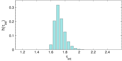
Finally we analyse the impact of the initial configuration ๐›(0)superscript๐›0\mathbf{b}^{(0)}. To this end we perform L๐ฟL elementary NESA runs of length 2โ€‹N2๐‘2N, all starting from the initial bond configuration ๐›0subscript๐›0\mathbf{b}_{0} with fixed threshold ฮปโˆ—superscript๐œ†\lambda^{*} (as before) and from all L๐ฟL final configurations we pick the one with the least likelihood and use it as new initial configuration ๐›(0)superscript๐›0\mathbf{b}^{(0)}. For M๐‘€M different initial configurations thus determined we compute individually the integrated autocorrelation times. The actual numbers used are N=L=100๐‘๐ฟ100N=L=100 and M=1000๐‘€1000M=1000. The histogram of the integrated correlation times ฯ„ยฏiโ€‹nโ€‹tsubscriptยฏ๐œ๐‘–๐‘›๐‘ก\overline{\tau}_{int} of a 16ร—16161616\times 16 system for q=10๐‘ž10q=10 is shown in figure 1.

Refer to caption
Figure 1: Histogram of the integrated correlation times ฯ„ยฏiโ€‹nโ€‹tsubscriptยฏ๐œ๐‘–๐‘›๐‘ก\overline{\tau}_{int} corresponding to the autocorrelation function in Eq.โ€‰(62) for a 16ร—16161616\times 16 Potts model with q=10๐‘ž10q=10.

Obviously, the for the 16ร—16161616\times 16 system, the mean of the distribution is roughly 1.751.751.75 with a small standard deviation. For other system sizes and q๐‘žq-values we make essentially the same observation. So we can make the important conclusion that there is essentially no autocorrelation in that part of NESA, where we sample according to the constraint prior. That may sound surprising since the SW algorithm is known to mix slowly for the Potts model with q>4๐‘ž4q>4 [29], but this is only the case near the transition temperature ๐•“๐•“\mathbbm{b}. Moreover, in NESA the elements of the Markov chain, ฮปnโˆ—superscriptsubscript๐œ†๐‘›\lambda_{n}^{*}, do not really follow from the SW trajectory of a single walker, but there are jumps between walkers, that additionally lead to de-correlation.

4.3 Performance of nested sampling

We are interested in the dependence of the partition function on the inverse temperature ฮฒ๐›ฝ\beta, as it provides the entire thermodynamic information of the system. As emphasized before, the dependence of lnโก(Zโ€‹(๐•“))๐‘๐•“\ln(Z(\mathbbm{b})) on ๐•“๐•“\mathbbm{b} (for ๐•“>๐•“โˆ—๐•“superscript๐•“\mathbbm{b}>\mathbbm{b}^{*}, i.e. ฮบ>0๐œ…0\kappa>0) can be obtained from a single NESA run.
Refer to caption
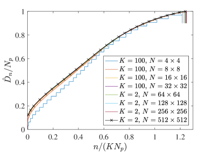
Figure 2: Dnโˆ—subscriptsuperscript๐ท๐‘›D^{*}_{n} for the q=10๐‘ž10q=10 Potts model with K=2๐พ2K=2 and K=100๐พ100K=100 and k=1๐‘˜1k=1 for various system sizes. The short vertical bars at the end mark nmaxsubscript๐‘›maxn_{\text{max}}.

Instead of generating the increasing sequence of likelihood values, we can equally well generate the corresponding increasing sequence of the active bonds numbers Dnsubscript๐ท๐‘›D_{n}. The upper limit of the number of active bonds Dmaxsubscript๐ทmaxD_{\text{max}} is equal to the number of pairs Npsubscript๐‘pN_{\text{p}}. In Fig.โ€‰2 we depict the fraction Dnโˆ—/Npsubscriptsuperscript๐ท๐‘›subscript๐‘pD^{*}_{n}/N_{\text{p}} versus n/(Kโ€‹Np)๐‘›๐พsubscript๐‘pn/(KN_{\text{p}}) for various system sizes and walkers. All plots are obtained for k=1๐‘˜1k=1, i.e. in each NESA step, one walker was updated. Obviously, with increasing system size the results rapidly converge towards a universal curve. An important finding is that the number of NESA steps nmaxsubscript๐‘›maxn_{\text{max}} it takes to reach Dmaxsubscript๐ทmaxD_{\text{max}} is proportional to the number of pairs and the number of walkers. A separate study for kโˆˆ{1,โ€ฆ,10}๐‘˜1โ€ฆ10k\in\{1,\ldots,10\} and qโˆˆ{2,โ€ฆ,10}๐‘ž2โ€ฆ10q\in\{2,\ldots,10\} yields the following scaling behavior

nmaxsubscript๐‘›max\displaystyle n_{\text{max}} =(a+bโ€‹q+cโ€‹q2)โ€‹Kโ€‹Npk,absent๐‘Ž๐‘๐‘ž๐‘superscript๐‘ž2๐พsubscript๐‘p๐‘˜\displaystyle=(a+bq+cq^{2})\frac{KN_{\text{p}}}{k}\;, (63)

with a=0.606,b=0.096,c=โˆ’0.003formulae-sequence๐‘Ž0.606formulae-sequence๐‘0.096๐‘0.003a=0.606,b=0.096,c=-0.003 for a 8ร—8888\times 8 system and a=0.599,b=0.089,c=โˆ’0.002formulae-sequence๐‘Ž0.599formulae-sequence๐‘0.089๐‘0.002a=0.599,b=0.089,c=-0.002 for a 16ร—16161616\times 16 system. We find that the q๐‘žq-dependent prefactor is nearly independent of the system size and it is a very smooth function in q๐‘žq. There is no distinction in the behaviour for systems that have a first or second order phase transition. The key message so far is, however, that NESA needs Oโ€‹(1)โ€‹Kโ€‹Npk๐‘‚1๐พsubscript๐‘p๐‘˜O(1)\frac{KN_{\text{p}}}{k} steps. An rigorous analytic proof of this finding is given in appendix 6.3.

4.4 Properties of the threshold values Dnโˆ—subscriptsuperscript๐ท๐‘›D^{*}_{n}

Next we shall study the properties of the threshold values Dnโˆ—subscriptsuperscript๐ท๐‘›D^{*}_{n} for the case k=1๐‘˜1k=1. The results for various system sizes and walker numbers are shown in Fig.โ€‰2. We see that Dnโˆ—subscriptsuperscript๐ท๐‘›D^{*}_{n} represents a stairway with steps that have an average height of โ‰ˆ1absent1\approx 1 and average width of โ‰ˆKabsent๐พ\approx K. We denote the position, at which the ฮฝ๐œˆ\nu-th step begins, by nฮฝsubscript๐‘›๐œˆn_{\nu} and the corresponding height by Dnฮฝโˆ—subscriptsuperscript๐ทsubscript๐‘›๐œˆD^{*}_{n_{\nu}}. Based on Eq.โ€‰(41) we find โŸจฮ”โ€‹XnโŸฉ=ฮพnโ€‹(1โˆ’ฮพ)delimited-โŸจโŸฉฮ”subscript๐‘‹๐‘›superscript๐œ‰๐‘›1๐œ‰\left\langle\Delta X_{n}\right\rangle=\xi^{n}(1-\xi) and the mean partition function can then be written as

โŸจZNESAโ€‹(๐•“)โŸฉdelimited-โŸจโŸฉsubscript๐‘NESA๐•“\displaystyle\left\langle Z_{\text{NESA}}(\mathbbm{b})\right\rangle =โˆ‘ฮฝSฮฝ,withย โ€‹Sฮฝ:=eฮบโ€‹Dnฮฝโˆ—โ€‹(ฮพnฮฝโˆ’ฮพnฮฝ+1)formulae-sequenceabsentsubscript๐œˆsubscript๐‘†๐œˆassignwithย subscript๐‘†๐œˆsuperscript๐‘’๐œ…subscriptsuperscript๐ทsubscript๐‘›๐œˆsuperscript๐œ‰subscript๐‘›๐œˆsuperscript๐œ‰subscript๐‘›๐œˆ1\displaystyle=\sum_{\nu}S_{\nu}\;,\qquad\text{with }\;\;S_{\nu}:=e^{\kappa D^{*}_{n_{\nu}}}\;(\xi^{n_{\nu}}-\xi^{n_{\nu+1}}) (64)

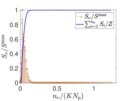
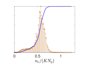
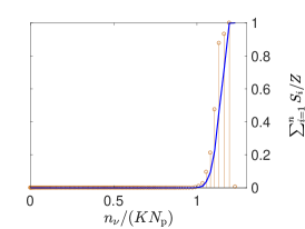
The summand Sฮฝsubscript๐‘†๐œˆS_{\nu} represents the contribution of the ฮฝ๐œˆ\nu-th step to the partition function, which clearly depends on temperature. In Fig.โ€‰3 the normalized summands Sฮฝ/Smaxsubscript๐‘†๐œˆsuperscript๐‘†maxS_{\nu}/S^{\text{max}} (Smax=maxฮผโกSฮผsuperscript๐‘†maxsubscript๐œ‡subscript๐‘†๐œ‡S^{\text{max}}=\max_{\mu}S_{\mu}) are plotted as function of the step position nฮฝsubscript๐‘›๐œˆn_{\nu} scaled by Kโ€‹Np๐พsubscript๐‘pKN_{\text{p}} for three inverse temperatures, below, at, and above the critical temperature ๐•“csubscript๐•“๐‘\mathbbm{b}_{c}.

Refer to caption
Refer to caption
Refer to caption
Figure 3: Summands Sฮฝsubscript๐‘†๐œˆS_{\nu} of Eq.โ€‰(64) and the corresponding cumulative sums for a q=10๐‘ž10q=10 Potts model on a 8ร—8888\times 8 lattice at different temperatures (from left to right): ๐•“=1๐•“1\mathbbm{b}=1, ๐•“c=๐•“csubscript๐•“๐‘subscript๐•“๐‘\mathbbm{b}_{c}=\mathbbm{b}_{c}, ๐•“=4๐•“4\mathbbm{b}=4. With increasing ๐•“๐•“\mathbbm{b} the main contribution to the sum shifts from the far left to the far right.

For ๐•“=1๐•“1\mathbbm{b}=1 one observes that only a small fraction of the stairway in Fig.โ€‰2 is sufficient for a converged result. For ๐•“csubscript๐•“๐‘\mathbbm{b}_{c} already a significant fraction is required and for ๐•“=4๐•“4\mathbbm{b}=4 the last summands clearly dominate the partition function. Hence for low temperatures (large ๐•“๐•“\mathbbm{b}) an accurate estimate for the partition function is only possible, if the NESA algorithm reaches the maximal number of active bonds Dnโˆ—=Npsubscriptsuperscript๐ท๐‘›subscript๐‘pD^{*}_{n}=N_{\text{p}}. Therefore the CPU-time scales like N2superscript๐‘2N^{2}, because the number of NESA steps required to reach the maximum likelihood value is nmaxsubscript๐‘›maxn_{\text{max}}, which is proportional to N๐‘N, and each NESA step involves one Swendsen-Wang update, which also scales like N๐‘N, if WQUPC is used for the cluster identification.

4.5 Partition function

We are now in the position to determine the yet unknown prior normalization Zฯ€subscript๐‘๐œ‹Z_{\pi} within the same NESA run. According to Eq.โ€‰(54) we need ZNESAโ€‹(๐•“โ†’โˆž)subscript๐‘NESAโ†’๐•“Z_{\text{NESA}}(\mathbbm{b}\to\infty). For ๐•“โ†’โˆžโ†’๐•“\mathbbm{b}\to\infty we have ฮบ=๐•“๐œ…๐•“\kappa=\mathbbm{b} and Eq.โ€‰(33) yields

ZNESAโ€‹(๐•“)subscript๐‘NESA๐•“\displaystyle Z_{\text{NESA}}(\mathbbm{b}) =โˆ‘n=0โˆže๐•“โ€‹Dnโˆ—โ€‹ฮ”โ€‹Xn,absentsuperscriptsubscript๐‘›0superscript๐‘’๐•“subscriptsuperscript๐ท๐‘›ฮ”subscript๐‘‹๐‘›\displaystyle=\sum_{n=0}^{\infty}e^{\mathbbm{b}D^{*}_{n}}\Delta X_{n}\;, (65)

from which for ๐•“โ†’โˆžโ†’๐•“\mathbbm{b}\to\infty only the terms with the maximal value of Dnโˆ—subscriptsuperscript๐ท๐‘›D^{*}_{n} (i.e. Dnโˆ—=Npsubscriptsuperscript๐ท๐‘›subscript๐‘๐‘D^{*}_{n}=N_{p}) determines the result, which is the case for nโ‰ฅnmax๐‘›subscript๐‘›maxn\geq n_{\text{max}}. We therefore have

ZNESAโ€‹(๐•“)subscript๐‘NESA๐•“\displaystyle Z_{\text{NESA}}(\mathbbm{b}) โŸถ๐•“โ†’โˆžโ€‹e๐•“โ€‹Npโ€‹โˆ‘n=nmaxโˆžฮ”โ€‹Xn.โ†’๐•“โŸถsuperscript๐‘’๐•“subscript๐‘๐‘superscriptsubscript๐‘›subscript๐‘›maxฮ”subscript๐‘‹๐‘›\displaystyle\underset{\mathbbm{b}\to\infty}{\longrightarrow}e^{\mathbbm{b}N_{p}}\;\sum_{n=n_{\text{max}}}^{\infty}\Delta X_{n}\;. (66)

The latter sum yields

โˆ‘n=nmaxโˆžฮ”โ€‹Xnsuperscriptsubscript๐‘›subscript๐‘›maxฮ”subscript๐‘‹๐‘›\displaystyle\sum_{n=n_{\text{max}}}^{\infty}\Delta X_{n} =limLโ†’โˆžโˆ‘n=nmaxLฮ”โ€‹Xn=Xnmax,absentsubscriptโ†’๐ฟsuperscriptsubscript๐‘›subscript๐‘›max๐ฟฮ”subscript๐‘‹๐‘›subscript๐‘‹subscript๐‘›max\displaystyle=\lim_{L\to\infty}\sum_{n=n_{\text{max}}}^{L}\Delta X_{n}=X_{n_{\text{max}}}\;, (67)

and we find for Eq.โ€‰(54)

lnโก(Zฯ€)subscript๐‘๐œ‹\displaystyle\ln\big{(}Z_{\pi}\big{)} =lnโกqโˆ’lnโกXnmax.absent๐‘žsubscript๐‘‹subscript๐‘›max\displaystyle=\ln q-\ln X_{n_{\text{max}}}\;. (68)

Inserting this result in Eq.โ€‰(52) yields

lnโก(ZPโ€‹(๐•“))subscript๐‘P๐•“\displaystyle\ln\big{(}Z_{\text{P}}(\mathbbm{b})\big{)} =lnโกqโˆ’lnโกXnmaxโˆ’๐•“โ€‹Np+lnโก(ZNESAโ€‹(๐•“)).absent๐‘žsubscript๐‘‹subscript๐‘›max๐•“subscript๐‘๐‘subscript๐‘NESA๐•“\displaystyle=\ln q-\ln X_{n_{\text{max}}}-\mathbbm{b}N_{p}+\ln\big{(}Z_{\text{NESA}}(\mathbbm{b})\big{)}\;. (69)

In particular for ๐•“=๐•“โˆ—๐•“superscript๐•“\mathbbm{b}=\mathbbm{b}^{*} (i.e. ฮบ=0๐œ…0\kappa=0) we have

lnโก(ZPโ€‹(๐•“โˆ—))subscript๐‘Psuperscript๐•“\displaystyle\ln\big{(}Z_{\text{P}}(\mathbbm{b}^{*})\big{)} =lnโกqโˆ’lnโกXnmaxโˆ’๐•“โˆ—โ€‹Np.absent๐‘žsubscript๐‘‹subscript๐‘›maxsuperscript๐•“subscript๐‘๐‘\displaystyle=\ln q-\ln X_{n_{\text{max}}}-\mathbbm{b}^{*}N_{p}\;. (70)

Since lnโก(ZP)subscript๐‘P\ln(Z_{\text{P}}) is an extensive quantity in the thermodynamic limit, for all temperatures, for large N๐‘N we therefore find

lnโกXnmaxโˆN.proportional-tosubscript๐‘‹subscript๐‘›max๐‘\displaystyle\ln X_{n_{\text{max}}}\propto N\;. (71)

This expression is used in the numerical evaluation of lnโก(ZPโ€‹(๐•“))subscript๐‘P๐•“\ln(Z_{\text{P}}(\mathbbm{b})). lnโก(Xnmax)subscript๐‘‹subscript๐‘›max\ln(X_{n_{\text{max}}}) turns out to play a crucial role, also in the following considerations. Its properties are studied analytically in appendix 6.4. For an initial qualitative discussion we use Eq.โ€‰(158) and Eq.โ€‰(45) to compute the mean of lnโก(Xnmax)subscript๐‘‹subscript๐‘›max\ln(X_{n_{\text{max}}}), which is โŸจlnโก(Xnmax)โŸฉ=โˆ’nmaxโ€‹kKdelimited-โŸจโŸฉsubscript๐‘‹subscript๐‘›maxsubscript๐‘›max๐‘˜๐พ\left\langle\ln(X_{n_{\text{max}}})\right\rangle=-n_{\text{max}}\frac{k}{K}, and Eq.โ€‰(68) turns into

lnโก(Zฯ€)subscript๐‘๐œ‹\displaystyle\ln\big{(}Z_{\pi}\big{)} =lnโกq+nmaxโ€‹kK.absent๐‘žsubscript๐‘›max๐‘˜๐พ\displaystyle=\ln q+n_{\text{max}}\frac{k}{K}\;. (72)

Based on our finding, nmax=ฮฑโ€‹Npโ€‹Kksubscript๐‘›max๐›ผsubscript๐‘๐‘๐พ๐‘˜n_{\text{max}}=\alpha\frac{N_{p}K}{k}, we obtain

lnโก(Zฯ€)Npsubscript๐‘๐œ‹subscript๐‘๐‘\displaystyle\frac{\ln\big{(}Z_{\pi}\big{)}}{N_{p}} =lnโกqNp+ฮฑ,absent๐‘žsubscript๐‘๐‘๐›ผ\displaystyle=\frac{\ln q}{N_{p}}+\alpha\;, (73)

where ฮฑ=Oโ€‹(1)๐›ผ๐‘‚1\alpha=O(1). We see that in the thermodynamic limit lnโก(Zฯ€โ€‹(ฮฒ))โ†’ฮฑโ€‹Npโ†’subscript๐‘๐œ‹๐›ฝ๐›ผsubscript๐‘๐‘\ln\big{(}Z_{\pi}(\beta)\big{)}\to\alpha N_{p}, which is consistent with the requirement that lnโก(Zฯ€โ€‹(ฮฒ))subscript๐‘๐œ‹๐›ฝ\ln\big{(}Z_{\pi}(\beta)\big{)} is an extensive quantity, as it is proportional to the free energy. Moreover, it will be shown in this section, the relative statistical uncertainty of lnโก(Xnmax)subscript๐‘‹subscript๐‘›max\ln(X_{n_{\text{max}}}) is proportional to 1/Nโ€‹K1๐‘๐พ1/\sqrt{NK}, and therefore Zฯ€subscript๐‘๐œ‹Z_{\pi} can be determined for large systems from a single NESA run with high accuracy.
Refer to caption
Refer to caption
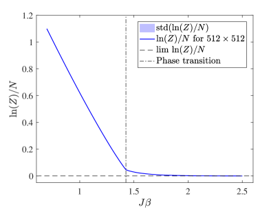
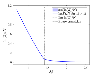
Figure 4: lnโก(Z)/N๐‘๐‘\ln(Z)/N for a q=10 system versus ๐•“๐•“\mathbbm{b} evaluated via nested sampling with K=100๐พ100K=100 and Npr=500subscript๐‘pr500N_{\text{pr}}=500 (left panel) and K=2๐พ2K=2 and Npr=500subscript๐‘pr500N_{\text{pr}}=500 (right panel) walkers. The inverse critical temperature ๐•“csubscript๐•“๐‘\mathbbm{b}_{c} is marked by a vertical chain line and the exact limit value for ๐•“โ†’โˆžโ†’๐•“\mathbbm{b}\to\infty (see Eq.โ€‰(3)) is represented by a dashed line. System sizes are 16ร—16161616\times 16 (left panel) and 512ร—512512512512\times 512 (right panel).

Fig.โ€‰4 displays lnโก(Z)/N๐‘๐‘\ln(Z)/N versus ๐•“๐•“\mathbbm{b} for the 10-state Potts model for the system sizes 16ร—16161616\times 16 and 512ร—512512512512\times 512. For large systems, the statistical uncertainties are smaller than the line thickness. The inverse temperature of the phase transition for an infinite 2d square lattice as given in Eq.โ€‰(4) is indicated by a vertical line. Above ๐•“csubscript๐•“๐‘\mathbbm{b}_{c}, the curve approaches rapidly the limiting value of lnโก(Z)/N=lnโก(q)/N๐‘๐‘๐‘ž๐‘\ln(Z)/N=\ln(q)/N for ๐•“=โˆž๐•“\mathbbm{b}=\infty, which is depicted by a dashed horizontal line. We observe that the largest uncertainty occurs at the lowest value of ๐•“๐•“\mathbbm{b}, i.e. for ๐•“โˆ—superscript๐•“\mathbbm{b}^{*} which is reasonable as the value at ๐•“โ†’โˆžโ†’๐•“\mathbbm{b}\to\infty was fixed to the exact result. ๐•“โˆ—superscript๐•“\mathbbm{b}^{*} corresponds to ฮบ=0๐œ…0\kappa=0 and we have

ZPโ€‹(๐•“โˆ—)subscript๐‘Psuperscript๐•“\displaystyle Z_{\text{P}}(\mathbbm{b}^{*}) =Zฯ€โ€‹eโˆ’๐•“โˆ—โ€‹Npโ€‹limLโ†’โˆžโˆ‘n=0Lฮ”โ€‹XnโŸ=1absentsubscript๐‘๐œ‹superscript๐‘’superscript๐•“subscript๐‘๐‘subscriptโŸsubscriptโ†’๐ฟsuperscriptsubscript๐‘›0๐ฟฮ”subscript๐‘‹๐‘›absent1\displaystyle=Z_{\pi}e^{-\mathbbm{b}^{*}N_{p}}\underbrace{\lim_{L\to\infty}\sum_{n=0}^{L}\Delta X_{n}}_{\color[rgb]{0,0,1}=1} (74)
lnโก(ZPโ€‹(๐•“โˆ—))subscript๐‘Psuperscript๐•“\displaystyle\ln\big{(}Z_{\text{P}}(\mathbbm{b}^{*})\big{)} =lnโก(Zฯ€)โˆ’๐•“โˆ—โ€‹Np.absentsubscript๐‘๐œ‹superscript๐•“subscript๐‘๐‘\displaystyle=\ln\big{(}Z_{\pi}\big{)}-\mathbbm{b}^{*}N_{p}\;. (75)

Hence, the accuracy of lnโก(ZP)subscript๐‘P\ln(Z_{\text{P}}) at the inverse temperature ๐•“โˆ—superscript๐•“\mathbbm{b}^{*} is the same as that of lnโก(Zฯ€)subscript๐‘๐œ‹\ln(Z_{\pi}), which is dictated by the distribution of lnโก(Xnmax)subscript๐‘‹subscript๐‘›max\ln(X_{n_{\text{max}}}). Mean and variance of lnโก(Xnmax)subscript๐‘‹subscript๐‘›max\ln(X_{n_{\text{max}}}) are derived in appendix 6.4. Along with Eq.โ€‰(154) for nmaxsubscript๐‘›maxn_{\text{max}} and Eq.โ€‰(45) they are given by

โŸจlnโก(Xmax)โŸฉdelimited-โŸจโŸฉsubscript๐‘‹max\displaystyle\bigg{\langle}\ln\big{(}X_{\text{max}}\big{)}\bigg{\rangle} =โŸจnmaxโŸฉโ€‹โŸจl1โŸฉ=Lโˆ—absentdelimited-โŸจโŸฉsubscript๐‘›maxdelimited-โŸจโŸฉsubscript๐‘™1superscript๐ฟ\displaystyle=\langle n_{\text{max}}\rangle\;\langle l_{1}\rangle\;=L^{*} (76a)
and
โŸจ(ฮ”โ€‹lnโก(Xmax))2โŸฉdelimited-โŸจโŸฉsuperscriptฮ”subscript๐‘‹max2\displaystyle\bigg{\langle}\bigg{(}\Delta\ln\big{(}X_{\text{max}}\big{)}\bigg{)}^{2}\bigg{\rangle} =2โ€‹โŸจnmaxโŸฉโ€‹โŸจ(ฮ”โ€‹l1)2โŸฉ=2โ€‹Lโˆ—โ€‹โŸจ(ฮ”โ€‹l1)2โŸฉโŸจl1โŸฉ=2โ€‹Lโˆ—โ€‹k~โ€ฒk~โ€‹K.absent2delimited-โŸจโŸฉsubscript๐‘›maxdelimited-โŸจโŸฉsuperscriptฮ”subscript๐‘™122superscript๐ฟdelimited-โŸจโŸฉsuperscriptฮ”subscript๐‘™12delimited-โŸจโŸฉsubscript๐‘™12superscript๐ฟsuperscript~๐‘˜โ€ฒ~๐‘˜๐พ\displaystyle=2\;\langle n_{\text{max}}\rangle\;\langle\big{(}\Delta l_{1}\big{)}^{2}\rangle\;=2\;L^{*}\;\frac{\langle\big{(}\Delta l_{1}\big{)}^{2}\rangle}{\langle l_{1}\rangle}=\frac{2\;L^{*}\tilde{k}^{\prime}}{\tilde{k}K}\;. (76b)

The relative statistical uncertainty of lnโก(Xnmax)subscript๐‘‹subscript๐‘›max\ln(X_{n_{\text{max}}}) is therefore

ฮต=โŸจ(ฮ”โ€‹lnโก(Xmax))2โŸฉ|โŸจlnโก(Xmax)โŸฉ|๐œ€delimited-โŸจโŸฉsuperscriptฮ”subscript๐‘‹max2delimited-โŸจโŸฉsubscript๐‘‹max\displaystyle\varepsilon=\frac{\sqrt{\bigg{\langle}\bigg{(}\Delta\ln\big{(}X_{\text{max}}\big{)}\bigg{)}^{2}\bigg{\rangle}}}{\bigg{|}\bigg{\langle}\ln\big{(}X_{\text{max}}\big{)}\bigg{\rangle}\bigg{|}} =2โ€‹k~โ€ฒLโˆ—โ€‹k~โ€‹K.absent2superscript~๐‘˜โ€ฒsuperscript๐ฟ~๐‘˜๐พ\displaystyle=\sqrt{\frac{2\tilde{k}^{\prime}}{L^{*}\tilde{k}K}}\;. (77)

We recall that Lโˆ—=โˆ’lnโก(Xnmax)+Oโ€‹(k/K)superscript๐ฟsubscript๐‘‹subscript๐‘›max๐‘‚๐‘˜๐พL^{*}=-\ln(X_{n_{\text{max}}})+O(k/K), as defined in Eq.โ€‰(142), and, therefore, we have

lnโก(ZPโ€‹(๐•“โˆ—))subscript๐‘Psuperscript๐•“\displaystyle\ln\big{(}Z_{\text{P}}({\mathbbm{b}^{*}})\big{)} =lnโก(q)โˆ’Lโˆ—+Oโ€‹(k/K).absent๐‘žsuperscript๐ฟ๐‘‚๐‘˜๐พ\displaystyle=\ln(q)-L^{*}+O(k/K)\;. (78)

Since lnโก(ZPโ€‹(๐•“โˆ—))subscript๐‘Psuperscript๐•“\ln\big{(}Z_{\text{P}}({\mathbbm{b}^{*}})\big{)} is an extensive quantity, for large systems it has to be proportional to N๐‘N and, hence, Lโˆ—=fโ€‹(q)โ€‹Nsuperscript๐ฟ๐‘“๐‘ž๐‘L^{*}=f(q)N, with fโ€‹(q)๐‘“๐‘žf(q) being a constant, independent of N๐‘N, K๐พK, and k๐‘˜k, that will however depend on q๐‘žq. For the statistical uncertainty it means

ฮต=โŸจ(ฮ”โ€‹lnโก(Xmax))2โŸฉ|โŸจlnโก(Xmax)โŸฉ|๐œ€delimited-โŸจโŸฉsuperscriptฮ”subscript๐‘‹max2delimited-โŸจโŸฉsubscript๐‘‹max\displaystyle\varepsilon=\frac{\sqrt{\bigg{\langle}\bigg{(}\Delta\ln\big{(}X_{\text{max}}\big{)}\bigg{)}^{2}\bigg{\rangle}}}{\bigg{|}\bigg{\langle}\ln\big{(}X_{\text{max}}\big{)}\bigg{\rangle}\bigg{|}} =2โ€‹k~โ€ฒfโ€‹(q)โ€‹k~โ€‹Kโ€‹N.absent2superscript~๐‘˜โ€ฒ๐‘“๐‘ž~๐‘˜๐พ๐‘\displaystyle=\sqrt{\frac{2\tilde{k}^{\prime}}{f(q)\tilde{k}KN}}\;. (79)

The pleasant bottom line is that the relative uncertainty is proportional to 1/Nโ€‹K1๐‘๐พ1/\sqrt{NK}, and it decreases with increasing system size.

4.6 Internal energy

Given lnโก(Z)๐‘\ln(Z) as function of ๐•“๐•“\mathbbm{b} for a system in the canonical ensemble, thermodynamic quantities like the Helmholtz free energy F and the internal energy U as well as the entropy S๐‘†S and heat capacity cVsubscript๐‘๐‘‰c_{V} can be deduced [30]. Starting from the estimate of the partition function in Eq.โ€‰(35), expressions for the first and second derivative of lnโก(Z)๐‘\ln(Z) w. r. t. ๐•“๐•“\mathbbm{b} can be determined. Given these expressions we can evaluate the physical quantities analytically, based on the sequence of active bonds Dnโˆ—subscriptsuperscript๐ท๐‘›D^{*}_{n} from a single NESA run and the sample of prior masses. Hence we can avoid the determination of numerical derivatives and the associated errors. From Eq.โ€‰(53) we have

lnโก(Lโ€‹(๐›))๐ฟ๐›\displaystyle\ln(L(\mathbf{b})) =\displaystyle= ฮบโ€‹Dโ€‹(๐›).๐œ…๐ท๐›\displaystyle\kappa\;D(\mathbf{b})\;. (80)

Given the sequence Dnโˆ—subscriptsuperscript๐ท๐‘›D^{*}_{n} from a single NESA run and the corresponding prior masses ฮ”โ€‹Xnฮ”subscript๐‘‹๐‘›\Delta X_{n} we can calculate the logarithm of the partition function

lnโก(ZNESA)subscript๐‘NESA\displaystyle\ln(Z_{\text{NESA}}) =\displaystyle= lnโก(โˆ‘neฮบโ€‹Dnโˆ—โ€‹ฮ”โ€‹Xn)subscript๐‘›superscript๐‘’๐œ…subscriptsuperscript๐ท๐‘›ฮ”subscript๐‘‹๐‘›\displaystyle\ln\big{(}\sum_{n}e^{\kappa D^{*}_{n}}\>\Delta X_{n}\big{)} (81)

and the derivative with respect to ๐•“๐•“\mathbbm{b}

โˆ‚โˆ‚๐•“โ€‹lnโก(ZNESAโ€‹(๐•“))=11โˆ’eโˆ’๐•“โ€‹โˆ‘nDnโˆ—โ€‹eฮบโ€‹Dnโˆ—โ€‹ฮ”โ€‹XnZNESAโŸ=pn=J1โˆ’eโˆ’๐•“โ€‹โŸจDโŸฉ๐•“.๐•“subscript๐‘NESA๐•“absent11superscript๐‘’๐•“subscript๐‘›subscriptsuperscript๐ท๐‘›subscriptโŸsuperscript๐‘’๐œ…subscriptsuperscript๐ท๐‘›ฮ”subscript๐‘‹๐‘›subscript๐‘NESAabsentsubscript๐‘๐‘›missing-subexpressionabsent๐ฝ1superscript๐‘’๐•“subscriptdelimited-โŸจโŸฉ๐ท๐•“\displaystyle\begin{aligned} \frac{\partial}{\partial\mathbbm{b}}\>\ln(Z_{\text{NESA}}(\mathbbm{b}))&=\frac{1}{1-e^{-\mathbbm{b}}}\>\sum_{n}D^{*}_{n}\>\underbrace{\frac{e^{\kappa D^{*}_{n}}\>\>\Delta X_{n}}{Z_{\text{NESA}}}}_{\color[rgb]{0,0,1}=p_{n}}\\ &=\frac{J}{1-e^{-\mathbbm{b}}}\>\left\langle D\right\rangle_{\mathbbm{b}}\;.\end{aligned} (82)

According to Eq.โ€‰(52) we find e.g. for the internal energy

U๐‘ˆ\displaystyle U =โŸจHโŸฉ=โˆ’โˆ‚โˆ‚๐•“โ€‹lnโก(ZP)=Jโ€‹(Npโˆ’โŸจDโŸฉ๐•“1โˆ’eโˆ’๐•“).absentdelimited-โŸจโŸฉ๐ป๐•“subscript๐‘P๐ฝsubscript๐‘psubscriptdelimited-โŸจโŸฉ๐ท๐•“1superscript๐‘’๐•“\displaystyle=\left\langle H\right\rangle=-\frac{\partial}{\partial\mathbbm{b}}\>\ln(Z_{\text{P}})=J\bigg{(}N_{\text{p}}-\frac{\left\langle D\right\rangle_{\mathbbm{b}}}{1-e^{-\mathbbm{b}}}\bigg{)}\;. (83)

The mean number of active bonds is related to the mean number of nearest neighbour pairs with equal spin โŸจNeqโ€‹(๐ฌ)โŸฉ๐•“subscriptdelimited-โŸจโŸฉsubscript๐‘eq๐ฌ๐•“\left\langle N_{\text{eq}}(\mathbf{s})\right\rangle_{\mathbbm{b}} via โŸจDโŸฉ๐•“=pbโ€‹โŸจNeqโŸฉ๐•“subscriptdelimited-โŸจโŸฉ๐ท๐•“subscript๐‘bsubscriptdelimited-โŸจโŸฉsubscript๐‘eq๐•“\left\langle D\right\rangle_{\mathbbm{b}}=p_{\text{b}}\left\langle N_{\text{eq}}\right\rangle_{\mathbbm{b}}, with pbsubscript๐‘bp_{\text{b}} (see Eq.โ€‰(51)) being the probability that nearest neighbour pairs of equal spin form an active bond. Therefore, the internal energy can also be expressed as

U๐‘ˆ\displaystyle U =โˆ’Jโ€‹(โŸจNeqโŸฉ๐•“โˆ’Np),absent๐ฝsubscriptdelimited-โŸจโŸฉsubscript๐‘eq๐•“subscript๐‘p\displaystyle=-J\big{(}\left\langle N_{\text{eq}}\right\rangle_{\mathbbm{b}}-N_{\text{p}}\big{)}\;, (84)

which is in agreement with the relation U=โˆ’Jโ€‹โˆ‚โˆ‚๐•“โ€‹โŸจHโŸฉ๐‘ˆ๐ฝ๐•“delimited-โŸจโŸฉ๐ปU=-J\frac{\partial}{\partial\mathbbm{b}}\left\langle H\right\rangle and the definition of the Hamiltonian in Eq.โ€‰(1). The second derivative can be deduced similarly. Mean and variance of an observable ๐’ช๐’ช\mathcal{O}, in the present case U๐‘ˆU, can be calculated using a single NESA run in a way similar to Eq.โ€‰(47). A single run produces ๐€โˆ—superscript๐€{\boldsymbol{\lambda}}^{*} which determines the observable ๐’ชโ€‹(๐€โˆ—,๐œฝ(m))๐’ชsuperscript๐€superscript๐œฝ๐‘š\mathcal{O}({\boldsymbol{\lambda}}^{*},\boldsymbol{\theta}^{(m)}) given the prior masses ๐œฝ(m)superscript๐œฝ๐‘š\boldsymbol{\theta}^{(m)} drawn from Eq.โ€‰(40). Averaging over prior masses leads to

โŸจ๐’ชฮณโŸฉdelimited-โŸจโŸฉsuperscript๐’ช๐›พ\displaystyle\left\langle\mathcal{O}^{\gamma}\right\rangle =1Nprโ€‹โˆ‘m=1Npr๐’ชโ€‹(๐€โˆ—,๐œฝ(m))ฮณ.absent1subscript๐‘prsuperscriptsubscript๐‘š1subscript๐‘pr๐’ชsuperscriptsuperscript๐€superscript๐œฝ๐‘š๐›พ\displaystyle=\frac{1}{N_{\text{pr}}}\sum_{m=1}^{N_{\text{pr}}}\mathcal{O}({\boldsymbol{\lambda}}^{*},\boldsymbol{\theta}^{(m)})^{\gamma}\;. (85)

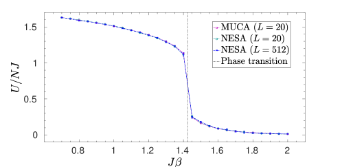
Fig.โ€‰5 shows the internal energy U๐‘ˆU versus ๐•“๐•“\mathbbm{b} for q=10๐‘ž10q=10 Potts systems computed via NESA and a MUCA simulation. For NESA at L=20๐ฟ20L=20 K=500๐พ500K=500 walkers and Npr=500subscript๐‘pr500N_{\text{pr}}=500 prior masses have been used and K=2๐พ2K=2 and Npr=500subscript๐‘pr500N_{\text{pr}}=500 for the L=512๐ฟ512L=512 system. The values agree excellently. For the MUCA simulation the Fortran code provided by Berg [3] is employed. For the comparison of the NESA results to the MUCA results from [3] the different definitions of ๐•“๐•“\mathbbm{b} and the Hamiltonian have to be taken into account.
Refer to caption
(a)
Figure 5: Internal energy U๐‘ˆU per site versus ๐•“๐•“\mathbbm{b} evaluated via nested sampling (K=500๐พ500K=500, Npr=500subscript๐‘pr500N_{\text{pr}}=500) and via multi-canonical sampling for the 20ร—20202020\times 20 and q=10๐‘ž10q=10 and via nested sampling (K=2๐พ2K=2, Npr=500subscript๐‘pr500N_{\text{pr}}=500) for the 512ร—512512512512\times 512 Potts system. The inverse critical temperature ๐•“csubscript๐•“๐‘\mathbbm{b}_{c} of the infinite system is marked by a vertical chain line.

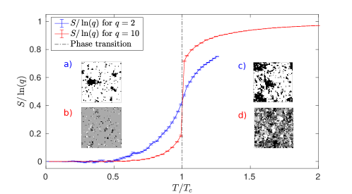
The qโ‰ค4๐‘ž4q\leq 4 Potts model exhibits a second order and the q>4๐‘ž4q>4 Potts model a first order phase transition. The difference in the order of the phase transition can be seen clearly in the discontinuity in the entropy

S=ฮฒโ€‹U+lnโกZ๐‘†๐›ฝ๐‘ˆ๐‘\displaystyle S=\beta U+\ln Z\; (86)

in Fig.โ€‰6. The snapshots in Fig.โ€‰6 show typical spin configurations slightly below and above the critical temperature for the second (q=2๐‘ž2q=2) and the first (q=10๐‘ž10q=10) order phase transition. Whereas there is little structural change in the spin configuration near to the phase transition in the second order case, in the first order phase transition the configuration slightly above Tcsubscript๐‘‡๐‘T_{c} is fluctuating while below Tcsubscript๐‘‡๐‘T_{c} one cluster dominates the system.

Refer to caption
(a)
Figure 6: Entropy for the q=2๐‘ž2q=2 (Ising-model) and q=10๐‘ž10q=10 Potts model at the L=64๐ฟ64L=64 system size calculated with K=512๐พ512K=512 walker and Npr=500subscript๐‘pr500N_{\text{pr}}=500 prior masses. The snapshots of typical spin configurations are at 0.99โ€‹Tc0.99subscript๐‘‡๐‘0.99\;T_{c} for q=2๐‘ž2q=2 (a) and q=10๐‘ž10q=10 (b) and at 1.01โ€‹Tc1.01subscript๐‘‡๐‘1.01\;T_{c} for q=2๐‘ž2q=2 (c) and q=10๐‘ž10q=10 (d).

4.7 Magnetic properties and phase transition

In order to compute magnetic properties of the Potts model we add a magnetic field term

HBsubscript๐ป๐ต\displaystyle H_{B} =โˆ’Bโ€‹โ„ณโ€‹(๐’”)absent๐ตโ„ณ๐’”\displaystyle=-B\;{\cal M}(\boldsymbol{s}) (87)

to the Hamiltonian. In this context, the magnetization of the spin configuration ๐’”๐’”\boldsymbol{s} is defined as

โ„ณโ€‹(๐’”)โ„ณ๐’”\displaystyle{\cal M}(\boldsymbol{s}) =โˆ‘ieiโ€‹2โ€‹ฯ€qโ€‹si.absentsubscript๐‘–superscript๐‘’๐‘–2๐œ‹๐‘žsubscript๐‘ ๐‘–\displaystyle=\sum_{i}e^{i\frac{2\pi}{q}s_{i}}\;. (88)

The definition Eq.โ€‰(88) has familiar limiting values. In the high temperature limit, where all spin-configurations have the same probability, we obtain

โŸจโ„ณโŸฉฮฒ=0,B=0subscriptdelimited-โŸจโŸฉโ„ณformulae-sequence๐›ฝ0๐ต0\displaystyle\langle\mathcal{M}\rangle_{\beta=0,B=0} =0for any system sizeย โ€‹N,absent0for any system sizeย ๐‘\displaystyle=0\;\qquad\text{for any system size }N, (89)
1Nโ€‹โŸจ|โ„ณ|โŸฉฮฒ=0,B=01๐‘subscriptdelimited-โŸจโŸฉโ„ณformulae-sequence๐›ฝ0๐ต0\displaystyle\frac{1}{N}\langle\big{|}\mathcal{M}\big{|}\rangle_{\beta=0,B=0} =0forย โ€‹Nโ†’โˆž.formulae-sequenceabsent0โ†’forย ๐‘\displaystyle=0\;\qquad\text{for }N\to\infty\;. (90)

The last equation follows from Eq.โ€‰(167) in appendix 6.5. In the opposite limit, Tโ†’0โ†’๐‘‡0T\to 0, all spins are equal. Here we have to distinguish the two observables. For โ„ณโ„ณ{\cal M}, we need to perform the thermodynamic limit Nโ†’โˆžโ†’๐‘N\to\infty before we reduce Bโ†’0โ†’๐ต0B\to 0. Then we find

โŸจโ„ณโŸฉNโ†’โˆž,T=0,Bโ†’0subscriptdelimited-โŸจโŸฉโ„ณformulae-sequenceโ†’๐‘formulae-sequence๐‘‡0โ†’๐ต0\displaystyle\langle{\cal M}\rangle_{N\to\infty,T=0,B\to 0} =N.absent๐‘\displaystyle=N\;. (91)

In case of the modulus, we can take B=0๐ต0B=0 also for a finite N๐‘N and obtain

โŸจ|โ„ณ|โŸฉN,T=0,B=0subscriptdelimited-โŸจโŸฉโ„ณformulae-sequence๐‘๐‘‡0๐ต0\displaystyle\langle\big{|}{\cal M}\big{|}\rangle_{N,T=0,B=0} =N.absent๐‘\displaystyle=N\;. (92)

The magnetization โŸจ|โ„ณ|โŸฉ/Ndelimited-โŸจโŸฉโ„ณ๐‘\langle\big{|}{\cal M}\big{|}\rangle/N for q=2๐‘ž2q=2 and q=10๐‘ž10q=10 is depicted in Fig.โ€‰7 for various system sizes. For the Ising model (q=2๐‘ž2q=2) we compare the NESA results to results obtained with a Markov Chain Monte Carlo algorithm with Swendsen Wang (SW) updates. For the infinite Ising model Onsagerโ€™s formula gives the exact solution for the susceptibility below Tcsubscript๐‘‡๐‘T_{c} which fits well to our calculations. The high temperature limits for the magnetization are derived in appendix 6.5.
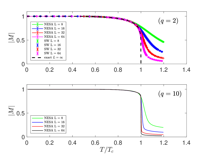
Refer to caption
(a)
Figure 7: Magnetization for the q=2๐‘ž2q=2 (upper panel) and q=10๐‘ž10q=10 (lower panel) Potts model for different system sizes. For comparison, the exact result for the q=2๐‘ž2q=2 case for the infinite system is also depicted. System parameters are K=1000,NS=100,Nb=1,Npr=1,Navg=10formulae-sequence๐พ1000formulae-sequencesubscript๐‘๐‘†100formulae-sequencesubscript๐‘๐‘1formulae-sequencesubscript๐‘pr1subscript๐‘avg10K=1000,N_{S}=100,N_{b}=1,N_{\text{pr}}=1,N_{\text{avg}}=10.

The behavior of the magnetization at the phase transition shows that the q=2๐‘ž2q=2 Potts model exhibits a second order and the q=10๐‘ž10q=10 Potts model a first order phase transition.

The thermodynamic expectation value of functions fโ€‹(โ„ณ)๐‘“โ„ณf({\cal M}) of the magnetization are defined by

โŸจfโ€‹(โ„ณ)โŸฉฮฒ,Bsubscriptdelimited-โŸจโŸฉ๐‘“โ„ณ๐›ฝ๐ต\displaystyle\langle f({\cal M})\rangle_{\beta,B} =1Zโ€‹โˆ‘๐’”e๐•“โ€‹โˆ‘โŸจiโ€‹jโŸฉฮดฯƒi,ฯƒj+ฮฒโ€‹Bโ€‹โ„ณโ€‹(๐’”)โ€‹fโ€‹(โ„ณโ€‹(๐’”)).absent1๐‘subscript๐’”superscript๐‘’๐•“subscriptdelimited-โŸจโŸฉ๐‘–๐‘—subscript๐›ฟsubscript๐œŽ๐‘–subscript๐œŽ๐‘—๐›ฝ๐ตโ„ณ๐’”๐‘“โ„ณ๐’”\displaystyle=\frac{1}{Z}\sum_{\boldsymbol{s}}e^{\mathbbm{b}\sum_{\langle ij\rangle}\delta_{\sigma_{i},\sigma_{j}}+\beta B{\cal M}(\boldsymbol{s})}\;f({\cal M}(\boldsymbol{s}))\;. (93)

The computation of expectation values in the framework of NESA in the Potts model is outlined in appendix 6.6. The standard expression for the susceptibility is

ฯ‡โ€‹(ฮฒ,B)๐œ’๐›ฝ๐ต\displaystyle\chi(\beta,B) =ฮฒNโ€‹(โŸจโ„ณ2โŸฉโˆ’โŸจโ„ณโŸฉ2).absent๐›ฝ๐‘delimited-โŸจโŸฉsuperscriptโ„ณ2superscriptdelimited-โŸจโŸฉโ„ณ2\displaystyle=\frac{\beta}{N}\bigg{(}\left\langle{\cal M}^{2}\right\rangle-\left\langle{\cal M}\right\rangle^{2}\bigg{)}\;. (94)

It has the drawback that for finite systems the magnetization vanishes for Bโ†’0โ†’๐ต0B\to 0 and, therefore, the susceptibility does not decrease for T๐‘‡T below Tcsubscript๐‘‡๐‘T_{c}. A more suitable estimate for the susceptibility for finite systems is given by [31]

ฯ‡|โ„ณ|โ€‹(ฮฒ,B)subscript๐œ’โ„ณ๐›ฝ๐ต\displaystyle\chi_{|{\cal M}|}(\beta,B) =ฮฒNโ€‹(โŸจโ„ณ2โŸฉโˆ’โŸจ|โ„ณ|โŸฉ2).absent๐›ฝ๐‘delimited-โŸจโŸฉsuperscriptโ„ณ2superscriptdelimited-โŸจโŸฉโ„ณ2\displaystyle=\frac{\beta}{N}\bigg{(}\left\langle{\cal M}^{2}\right\rangle-\left\langle|{\cal M}|\right\rangle^{2}\bigg{)}\;. (95)

Finally we plotted the susceptibility ฯ‡|โ„ณ|subscript๐œ’โ„ณ\chi_{|{\cal M}|} for the q=2๐‘ž2q=2 Potts model for the system sizes Lโˆˆ{8,16,32,64,128}๐ฟ8163264128L\in\{8,16,32,64,128\} in Fig.โ€‰8 and compare the nested sampling results with those obtained by the Swendsen Wang algorithm. First of all we observe a perfect agreement.
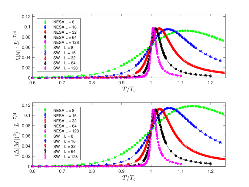
Refer to caption
(a)
Figure 8: Comparison of the susceptibility for the L={8,16,32,64,128}๐ฟ8163264128L=\{8,16,32,64,128\} Ising model as obtained by NESA and Swendsen Wang. The scaling factor Lฮณ/ฮฝsuperscript๐ฟ๐›พ๐œˆL^{\gamma/\nu} is already included and we have also plotted the variance of the magnetization . We recognize the correct scaling in the fact that the height of the peaks does not change for larger systems. System parameters are K=1000,NS=100,Nb=1,Npr=1,Navg=10formulae-sequence๐พ1000formulae-sequencesubscript๐‘๐‘†100formulae-sequencesubscript๐‘๐‘1formulae-sequencesubscript๐‘pr1subscript๐‘avg10K=1000,N_{S}=100,N_{b}=1,N_{\text{pr}}=1,N_{\text{avg}}=10.

Moreover, as expected, with increasing system size the resonance becomes narrower and is getting closer to the critical temperature of the infinite system, both scale as 1/L1๐ฟ1/L. We have scaled the susceptibility with Lฮณ/ฮฝsuperscript๐ฟ๐›พ๐œˆL^{\gamma/\nu} to show that the maximum values ฯ‡|โ„ณ|mโ€‹aโ€‹x/Lฮณ/ฮฝsubscriptsuperscript๐œ’๐‘š๐‘Ž๐‘ฅโ„ณsuperscript๐ฟ๐›พ๐œˆ\chi^{max}_{|{\cal M}|}/L^{\gamma/\nu} stay constant for larger system sizes for a critical exponent of ฮณ/ฮฝ=7/4๐›พ๐œˆ74\gamma/\nu=7/4, in agreement with the known finite size scaling, which is discussed in detail in [32, 31]. Next we turn to the critical exponent ฮณ/ฮฝ๐›พ๐œˆ\gamma/\nu that governs the behaviour of ฯ‡maxsubscript๐œ’max\chi_{\text{max}}, the maximum of susceptibility. We can either perform a non-linear fit of the maxima of ฯ‡๐œ’\chi obtained by NESA for the system sizes Lโˆˆ{8,16,32,64,128}๐ฟ8163264128L\in\{8,16,32,64,128\} with ฯ‡|โ„ณ|mโ€‹aโ€‹xโˆLฮณ/ฮฝproportional-tosubscriptsuperscript๐œ’๐‘š๐‘Ž๐‘ฅโ„ณsuperscript๐ฟ๐›พ๐œˆ\chi^{max}_{|{\cal M}|}\propto L^{\gamma/\nu}. This yields ฮณ/ฮฝ=1.754ยฑ0.002๐›พ๐œˆplus-or-minus1.7540.002\gamma/\nu=1.754\pm 0.002, while the fit of the maxima of โŸจ(ฮ”โ€‹|M|)2โŸฉdelimited-โŸจโŸฉsuperscriptฮ”๐‘€2\left\langle(\Delta|M|)^{2}\right\rangle yields ฮณ/ฮฝ=1.735ยฑ0.002๐›พ๐œˆplus-or-minus1.7350.002\gamma/\nu=1.735\pm 0.002. It should be pointed out that the scaling law โˆLฮณ/ฮฝproportional-toabsentsuperscript๐ฟ๐›พ๐œˆ\propto L^{\gamma/\nu} can still contain finite size corrections of the form โˆLฮณ/ฮฝโ€‹(1+Oโ€‹(1/L))proportional-toabsentsuperscript๐ฟ๐›พ๐œˆ1๐‘‚1๐ฟ\propto L^{\gamma/\nu}(1+O(1/L)). These corrections are clearly visible in figure 8 and it can also be seen with the naked eye that the finite size correction is more pronounced in โŸจ(ฮ”โ€‹|M|)2โŸฉdelimited-โŸจโŸฉsuperscriptฮ”๐‘€2\left\langle(\Delta|M|)^{2}\right\rangle. To eliminate the finite size corrections, we determining the slope of lnโก(ฯ‡maxโ€‹(L))=a+bโ€‹lnโก(L)subscript๐œ’max๐ฟ๐‘Ž๐‘๐ฟ\ln(\chi_{\text{max}}(L))=a+b\ln(L) for neighbouring system-sizes, plot the slope as function of 1/L1๐ฟ1/L and extrapolate to 1/Lโ†’0โ†’1๐ฟ01/L\to 0. This results in 1.75ยฑ0.01plus-or-minus1.750.011.75\pm 0.01 and 1.74ยฑ0.02plus-or-minus1.740.021.74\pm 0.02, for ฯ‡๐œ’\chi and โŸจ(ฮ”โ€‹|M|)2โŸฉdelimited-โŸจโŸฉsuperscriptฮ”๐‘€2\left\langle(\Delta|M|)^{2}\right\rangle respectively.

In addition to the susceptibility ฯ‡=ฮฒโ€‹โŸจ(ฮ”โ€‹|M|)2โŸฉ๐œ’๐›ฝdelimited-โŸจโŸฉsuperscriptฮ”๐‘€2\chi=\beta\left\langle(\Delta|M|)^{2}\right\rangle, we have also depicted the factor โŸจ(ฮ”โ€‹|M|)2โŸฉdelimited-โŸจโŸฉsuperscriptฮ”๐‘€2\left\langle(\Delta|M|)^{2}\right\rangle. Both terms have the same critical exponent ฮณ/ฮฝ๐›พ๐œˆ\gamma/\nu and differ only by the the way they approach the thermodynamic limit. It is clearly visible from the figure that ฯ‡๐œ’\chi approaches the thermodynamic limit of ฮณ/ฮฝ๐›พ๐œˆ\gamma/\nu from above, i.e. the height of the peaks in the upper plot monotonically increase with increasing system size, but the increase drops to zero with Nโ†’โˆžโ†’๐‘N\to\infty. This is in accord with the numerical value given above. On the other hand, โŸจ(ฮ”โ€‹|M|)2โŸฉdelimited-โŸจโŸฉsuperscriptฮ”๐‘€2\left\langle(\Delta|M|)^{2}\right\rangle approaches the thermodynamic limit from below. As defined in the appendix 6.6, there are two sample sizes Nbsubscript๐‘๐‘N_{b} and NSsubscript๐‘๐‘†N_{S}, which can both be set to 1, but in this case the statistical uncertainty has to be determined from repeated nested sampling runs. In this application it turned out to be favourable to replace the prior masses Xmsubscript๐‘‹๐‘šX_{m} by the mean values and to estimated the statistical noise by repeated NESA runs, which was necessary in any case to account for the statistical uncertainty introduced by the averages discussed in appendix 6.6. Otherwise, in all runs for figure Fig.โ€‰8 we have used K=1000๐พ1000K=1000 and Nb=1subscript๐‘๐‘1N_{b}=1 and NS=100subscript๐‘๐‘†100N_{S}=100. The later is necessary to reduce the statistical noise and it is faster than 100 repeated nested sampling runs. Then it occurs that the statistical noise is very small and the confidence intervals are determined from Navgsubscript๐‘avgN_{\text{avg}} repeated NESA runs. The reason why Nbsubscript๐‘๐‘N_{b} is already sufficient is due the the fact that in case of K=1000๐พ1000K=1000, the plateaus in Dnsubscript๐ท๐‘›D_{n} in Fig.โ€‰2 are roughly K๐พK, which is equivalent to using Nb=1000subscript๐‘๐‘1000N_{b}=1000.

4.8 Performance comparison multi-canonical sampling and nested sampling

For a proper comparison of MUCA and NESA we analyse the computing times needed for the calculation of lnโก(Z)/N๐‘๐‘\ln(Z)/N with a defined relative accuracy for the q=10๐‘ž10q=10 Potts model at the critical temperature ๐•“csubscript๐•“๐‘\mathbbm{b}_{c}. As derived in Sec. 4.5 the asymptotic behaviour of the relative accuracy in NESA is proportional to 1/Nโ€‹K1๐‘๐พ1/\sqrt{NK}. Fig.โ€‰9 shows the computed logarithmic relative uncertainty depending on the system size and the number of walker. The black solid line marks the relative accuracy of 101010~{}%. For each number of walker we do a line fit only for the data points below the 101010~{}%-line, because there the asymptotic behaviour should hold. We get nearly equidistant lines with a distance of ฮ”โ€‹lnโก(ฯต)โ‰ˆ0.69ฮ”italic-ฯต0.69\Delta\ln(\epsilon)\approx 0.69 and a slope of approximately โˆ’0.50.5-0.5 which confirms the scaling law derived analytically.
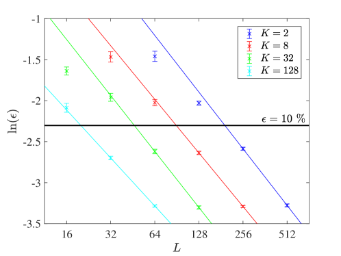
Refer to caption
(a)
Figure 9: Logarithm of the relative accuracy of lnโก(Z)/N๐‘๐‘\ln(Z)/N for the q=10 Potts model at ๐•“=๐•“c๐•“subscript๐•“๐‘\mathbbm{b}=\mathbbm{b}_{c} computed by nested sampling in dependence of the logarithmic grid-size and the number of walker K๐พK.

For the comparison of MUCA and NESA we analyse the scaling exponent x๐‘ฅx of the computing time tโˆNxproportional-to๐‘กsuperscript๐‘๐‘ฅt\propto N^{x} needed for calculating lnโก(Z)/N๐‘๐‘\ln(Z)/N with a relative accuracy of at least 101010~{}%. In MUCA we used a sample of 100 independent walker and stopped the computation when the requested relative accuracy is reached. We have implemented the MUCA simulation using local updates and found it scales with x=2.36ยฑ0.11๐‘ฅplus-or-minus2.360.11x=2.36\pm 0.11, see blue line in Fig.โ€‰10, which is consistent with the scaling of xโ‰ˆ2.3๐‘ฅ2.3x\approx 2.3 obtained in [2] for the same system. Here we have neglected the time needed for computing the weights needed for MUCA which scales with N2superscript๐‘2N^{2}.

Refer to caption
(a)
Figure 10: Logarithmic time for computing lnโก(Z)๐‘\ln(Z) versus the logarithmic grid size for the q=10 Potts model at ๐•“=๐•“c๐•“subscript๐•“๐‘\mathbbm{b}=\mathbbm{b}_{c} exhibits a slightly stronger scaling for MUCA than for NESA.

In NESA we found that the computing time scales with xโ‰ˆ2๐‘ฅ2x\approx 2 if we use a constant number of walker for every system size, see red line in Fig.โ€‰10. The scaling can be explained by the SW updates needed in each step scaling with kโ€‹N๐‘˜๐‘kN and the maximum number of steps scaling with Kโ€‹N/k๐พ๐‘๐‘˜KN/k, as discussed in section 4.3. Hence, the total time scales like tโˆKโ€‹N2proportional-to๐‘ก๐พsuperscript๐‘2t\propto KN^{2}. But, as pointed out before, decreasing the number of walker for increasing system sizes produces the same relative accuracy. Therefore we have a linear scaling in this case, tโˆฯต2โ€‹Nproportional-to๐‘กsuperscriptitalic-ฯต2๐‘t\propto\epsilon^{2}N. We performed calculations for L={16,32,64,128,256,512}๐ฟ163264128256512L=\{16,32,64,128,256,512\} at K={256,128,32,8,2,2}๐พ25612832822K=\{256,128,32,8,2,2\} which ensures that the relative accuracy is lower than 101010~{}% and we get a linear scaling in the region where K๐พK can be decreased and a quadratic scaling otherwise, see green line in Fig.โ€‰10. Additional to the smaller scaling exponent of NESA also the prefactor is smaller compared to MUCA.

4.9 Parallel nested sampling

As outlined in Sec. 4.5 the greatest uncertainty occurs at ๐•“โˆ—=lnโก(2)superscript๐•“2\mathbbm{b}^{*}=\ln(2) and the corresponding relative uncertainty is given in Eq.โ€‰(79). For kโ‰ชKmuch-less-than๐‘˜๐พk\ll K we have k~=k~โ€ฒ~๐‘˜superscript~๐‘˜โ€ฒ\tilde{k}=\tilde{k}^{\prime} and then

ฮต๐œ€\displaystyle\varepsilon =2fโ€‹(q)โ€‹Nโ€‹K.absent2๐‘“๐‘ž๐‘๐พ\displaystyle=\sqrt{\frac{2}{f(q)NK}}\;. (96)

Hence, the relative uncertainty behaves like 1/Nโ€‹K1๐‘๐พ1/\sqrt{NK}, independent of k๐‘˜k, which is corroborated by our numerical results shown in Fig.โ€‰9. This result deviates from the conjecture of Henderson et al. [17] that the uncertainty increases with k๐‘˜\sqrt{k}, based on the increasing variance of a single shrinkage factor โŸจ(ฮ”โ€‹l1)2โŸฉdelimited-โŸจโŸฉsuperscriptฮ”subscript๐‘™12\langle(\Delta l_{1})^{2}\rangle. This is fortunately not the case for the present application. As the uncertainty is independent of k๐‘˜k, NESA is perfectly suited for a parallel implementation. The k๐‘˜k walkers are drawn independently from each other according to the prior and this step consumes for large systems the lionโ€™s share for the CPU time.

5 Summary and conclusions

In this work we have evaluated the nested sampling (NESA) algorithm in the frame of the Potts model on a 2d square lattice for different system sizes and numbers of possible spin values q๐‘žq. Results and performance are compared with the established multi-canonical (MUCA) sampling method. We have employed the Fortuin and Kasteleyn bond representation. The primary goal was the computation of the partition function, which is difficult to determine reliably by standard Monte Carlo techniques. Both methods, multi-canonical sampling and nested sampling, exhibit a power law scaling of the computation time with increasing system-size. We find an exponent of 222 for NESA, while it is โ‰ˆ2.3absent2.3\approx 2.3 for MUCA, demonstrating the superiority of nested sampling. Moreover, in NESA the relative uncertainty of the logarithmic partition function scales with 1/N1๐‘1/\sqrt{N}, which allows to obtain very accurate results for large system sizes. Another advantage of nested sampling is that it can easily be implemented and does not require additional adjustments, like the weights wโ€‹(E)๐‘ค๐ธw(E) in MUCA, which becomes increasingly cumbersome with increasing system size.

Besides the evaluation of the partition function, we have demonstrated that it is possible to directly compute thermodynamic expectation values with NESA, both for observables that can be expressed entirely in the bond representation (improved estimators) and those that still need the original spin representation. Results were given for the internal energy, entropy, Helmholtz free energy, magnetization and magnetic susceptibility, for which we determined the critical exponent for the Ising model. In all cases we we found excellent agreement between the NESA results and those obtained by MUCA or the Swendsen-Wang algorithm.

In addition nested sampling is perfectly suited for parallel computing. In summary we have found that nested sampling is able to deal efficiently with problems that exhibit first order phase transitions. The method is a promising alternative to the multi-canonical algorithm, which is a state of the art computational technique for dealing with Potts-type of models. In our opinion nested sampling represents a high potential for applications in statistical physics and due to its uniqueness it deserves a place in a physicists standard repertoire of simulation techniques.

6 Appendix

6.1 Nested sampling the partion function

For the computation of integrals or sums of the form

Z๐‘\displaystyle Z =โˆ‘โˆซxโกLโ€‹(๐’™)โ€‹ฯ€โ€‹(๐’™),absentsubscript๐‘ฅ๐ฟ๐’™๐œ‹๐’™\displaystyle=\operatorname*{\mathchoice{\ooalign{$\displaystyle\sum$\cr$\displaystyle\int$\cr}}{\ooalign{\raisebox{0.14pt}{\scalebox{0.7}{$\textstyle\sum$}}\cr$\textstyle\int$\cr}}{\ooalign{\raisebox{0.2pt}{\scalebox{0.6}{$\scriptstyle\sum$}}\cr$\scriptstyle\int$\cr}}{\ooalign{\raisebox{0.2pt}{\scalebox{0.6}{$\scriptstyle\sum$}}\cr$\scriptstyle\int$\cr}}}\limits_{x}L(\boldsymbol{x})\pi(\boldsymbol{x})\;, (105)

where ฯ€โ€‹(๐’™)๐œ‹๐’™\pi(\boldsymbol{x}) represents a probability function, we introduce the dummy integral โˆซ๐‘‘ฮปโ€‹ฮดโ€‹(Lโ€‹(๐’™)โˆ’ฮป)=1differential-d๐œ†๐›ฟ๐ฟ๐’™๐œ†1\int d\lambda\delta(L(\boldsymbol{x})-\lambda)=1 and obtain after swapping the integrals

Z๐‘\displaystyle Z =โˆซ๐‘‘ฮปโ€‹ฮปโ€‹โˆ‘โˆซxโกฯ€โ€‹(๐’™)โ€‹ฮดโ€‹(Lโ€‹(๐’™)โˆ’ฮป).absentdifferential-d๐œ†๐œ†subscript๐‘ฅ๐œ‹๐’™๐›ฟ๐ฟ๐’™๐œ†\displaystyle=\int d\lambda\;\lambda\;\operatorname*{\mathchoice{\ooalign{$\displaystyle\sum$\cr$\displaystyle\int$\cr}}{\ooalign{\raisebox{0.14pt}{\scalebox{0.7}{$\textstyle\sum$}}\cr$\textstyle\int$\cr}}{\ooalign{\raisebox{0.2pt}{\scalebox{0.6}{$\scriptstyle\sum$}}\cr$\scriptstyle\int$\cr}}{\ooalign{\raisebox{0.2pt}{\scalebox{0.6}{$\scriptstyle\sum$}}\cr$\scriptstyle\int$\cr}}}\limits_{x}\;\pi(\boldsymbol{x})\;\delta(L(\boldsymbol{x})-\lambda)\;. (114)

The inner integral is related to the prior mass Xโ€‹(ฮป)๐‘‹๐œ†X(\lambda), which is defined as

Xโ€‹(ฮป)๐‘‹๐œ†\displaystyle X(\lambda) =โˆ‘โˆซ๐’™โกฯ€โ€‹(๐’™)โ€‹ฮธโ€‹(Lโ€‹(๐’™)โˆ’ฮป),absentsubscript๐’™๐œ‹๐’™๐œƒ๐ฟ๐’™๐œ†\displaystyle=\operatorname*{\mathchoice{\ooalign{$\displaystyle\sum$\cr$\displaystyle\int$\cr}}{\ooalign{\raisebox{0.14pt}{\scalebox{0.7}{$\textstyle\sum$}}\cr$\textstyle\int$\cr}}{\ooalign{\raisebox{0.2pt}{\scalebox{0.6}{$\scriptstyle\sum$}}\cr$\scriptstyle\int$\cr}}{\ooalign{\raisebox{0.2pt}{\scalebox{0.6}{$\scriptstyle\sum$}}\cr$\scriptstyle\int$\cr}}}\limits_{\boldsymbol{x}}\;\pi(\boldsymbol{x})\;\theta(L(\boldsymbol{x})-\lambda)\;, (123)

via

โˆ‘โˆซ๐’™โกฯ€โ€‹(๐’™)โ€‹ฮดโ€‹(Lโ€‹(๐’™)โˆ’ฮป)subscript๐’™๐œ‹๐’™๐›ฟ๐ฟ๐’™๐œ†\displaystyle\operatorname*{\mathchoice{\ooalign{$\displaystyle\sum$\cr$\displaystyle\int$\cr}}{\ooalign{\raisebox{0.14pt}{\scalebox{0.7}{$\textstyle\sum$}}\cr$\textstyle\int$\cr}}{\ooalign{\raisebox{0.2pt}{\scalebox{0.6}{$\scriptstyle\sum$}}\cr$\scriptstyle\int$\cr}}{\ooalign{\raisebox{0.2pt}{\scalebox{0.6}{$\scriptstyle\sum$}}\cr$\scriptstyle\int$\cr}}}\limits_{\boldsymbol{x}}\;\pi(\boldsymbol{x})\;\delta(L(\boldsymbol{x})-\lambda) =โˆ’ddโ€‹ฮปโ€‹Xโ€‹(ฮป).absent๐‘‘๐‘‘๐œ†๐‘‹๐œ†\displaystyle=-\frac{d}{d\lambda}X(\lambda)\;. (132)

Inserting this relation into Eq.โ€‰(114) yields

Z๐‘\displaystyle Z =โˆ’โˆซฮปโ€‹dโ€‹Xโ€‹(ฮป)dโ€‹ฮปโ€‹๐‘‘ฮป=โˆซโ„’โ€‹(X)โ€‹๐‘‘X,absent๐œ†๐‘‘๐‘‹๐œ†๐‘‘๐œ†differential-d๐œ†โ„’๐‘‹differential-d๐‘‹\displaystyle=-\int\lambda\;\frac{dX(\lambda)}{d\lambda}\;d\lambda=\int{\cal L}(X)\;dX\;, (133)

where โ„’โ€‹(X)โ„’๐‘‹{\cal L}(X) is the inverse function of Xโ€‹(ฮป)๐‘‹๐œ†X(\lambda). We have tacitly assumed that Xโ€‹(ฮป)๐‘‹๐œ†X(\lambda) and โ„’โ€‹(X)โ„’๐‘‹{\cal L}(X) are strictly monotonic functions. From the definition of the prior mass Xโ€‹(ฮป)๐‘‹๐œ†X(\lambda) it is clear that it decreases monotonically with increasing ฮป๐œ†\lambda. Therefore an additional minus sign appears in the last step due to switching the integration limits. It is, however, not always automatically ensured that Xโ€‹(ฮป)๐‘‹๐œ†X(\lambda) is strictly monotonic, but it can easily be added.

6.2 Nested sampling discrete configuration spaces

Here we will analyse some details of the algorithm outlined in section 3.2. In case of a discrete problem, some additional considerations are in order. We consider a discrete configuration space ๐’™๐’™\boldsymbol{x}. The corresponding likelihood Lโ€‹(๐’™)๐ฟ๐’™L(\boldsymbol{x}) values are also discrete and it can have the following values Lฮฝsubscript๐ฟ๐œˆL_{\nu}. The corresponding prior masses are

Xโ€‹(ฮป)๐‘‹๐œ†\displaystyle X(\lambda) =โˆ‘๐’™ฯ€โ€‹(๐’™)โ€‹ฮธโ€‹(Lโ€‹(๐’™)>ฮป)โ€‹โˆ‘ฮปฮฝฮดLโ€‹(๐’™),ฮปฮฝโŸ=1.absentsubscript๐’™๐œ‹๐’™๐œƒ๐ฟ๐’™๐œ†subscriptโŸsubscriptsubscript๐œ†๐œˆsubscript๐›ฟ๐ฟ๐’™subscript๐œ†๐œˆabsent1\displaystyle=\sum_{\boldsymbol{x}}\;\pi(\boldsymbol{x})\;\theta(L(\boldsymbol{x})>\lambda)\;\underbrace{\sum_{\lambda_{\nu}}\delta_{L(\boldsymbol{x}),\lambda_{\nu}}}_{\color[rgb]{0,0,1}=1}\;.
Xโ€‹(ฮป)๐‘‹๐œ†\displaystyle X(\lambda) =โˆ‘ฮปฮฝPโ€‹(ฮปฮฝ)โ€‹ฮธโ€‹(ฮปฮฝ>ฮป)absentsubscriptsubscript๐œ†๐œˆ๐‘ƒsubscript๐œ†๐œˆ๐œƒsubscript๐œ†๐œˆ๐œ†\displaystyle=\sum_{\lambda_{\nu}}\;P(\lambda_{\nu})\;\theta(\lambda_{\nu}>\lambda) (134)
Pโ€‹(ฮปฮฝ)๐‘ƒsubscript๐œ†๐œˆ\displaystyle P(\lambda_{\nu}) =โˆ‘๐’™ฯ€โ€‹(๐’™)โ€‹ฮดLโ€‹(๐’™),ฮปฮฝ.absentsubscript๐’™๐œ‹๐’™subscript๐›ฟ๐ฟ๐’™subscript๐œ†๐œˆ\displaystyle=\sum_{\boldsymbol{x}}\;\pi(\boldsymbol{x})\;\delta_{L(\boldsymbol{x}),\lambda_{\nu}}\;. (135)

Clearly, Xโ€‹(ฮป)๐‘‹๐œ†X(\lambda) is a discontinuous (open) stairway function as depicted in figure 11 and, therefore, the PDF of the prior mass is far from being uniform.
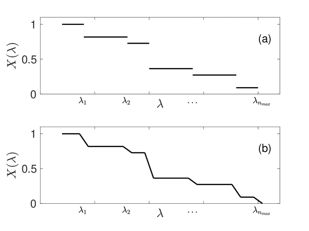
Refer to caption
Figure 11: Prior masses Xโ€‹(ฮป)๐‘‹๐œ†X(\lambda) versus likelihood value ฮป๐œ†\lambda for the purely discrete case configuration space (a) and the augmented case (b).

However, we show that the augmented configuration space introduced in section 4.1 to overcome degeneracy of the likelihood by an additional variable m๐‘šm with uniform PDF

pโ€‹(m)๐‘๐‘š\displaystyle p(m) =12โ€‹ฮตโ€‹ฮธโ€‹(โˆ’ฮตโ‰คm<ฮต)absent12๐œ€๐œƒ๐œ€๐‘š๐œ€\displaystyle=\frac{1}{2\varepsilon}\theta(-\varepsilon\leq m<\varepsilon)\; (136)

can be used to obtain a continuous Xโ€‹(ฮป)๐‘‹๐œ†X(\lambda). The augmented likelihood is Lโ€‹(๐’™,m)=Lโ€‹(๐’™)+m๐ฟ๐’™๐‘š๐ฟ๐’™๐‘šL(\boldsymbol{x},m)=L(\boldsymbol{x})+m. Next we compute the PDF for the likelihood values that occur in the algorithm with the augmented configurations

pโ€‹(ฮป|โ„)๐‘conditional๐œ†โ„\displaystyle p(\lambda\,\boldsymbol{|}\,{\cal I}) =โˆ‘๐’™โˆซ๐‘‘mโ€‹pโ€‹(m)โ€‹ฯ€โ€‹(๐’™)โ€‹pโ€‹(ฮป|๐’™,m,โ„)โŸ=ฮดโ€‹(ฮปโˆ’Lโ€‹(๐’™)โˆ’m)absentsubscript๐’™differential-d๐‘š๐‘๐‘š๐œ‹๐’™subscriptโŸ๐‘conditional๐œ†๐’™๐‘šโ„absent๐›ฟ๐œ†๐ฟ๐’™๐‘š\displaystyle=\sum_{\boldsymbol{x}}\int dm\;p(m)\pi(\boldsymbol{x})\underbrace{p(\lambda\,\boldsymbol{|}\,\boldsymbol{x},m,{\cal I})}_{\color[rgb]{0,0,1}=\delta(\lambda-L(\boldsymbol{x})-m)}
=โˆ‘ฮปฮฝ(โˆ‘๐’™ฯ€โ€‹(๐’™)โ€‹ฮดLโ€‹(๐’™),ฮปฮฝ)โ€‹(โˆซ๐‘‘mโ€‹pโ€‹(m)โ€‹ฮดโ€‹(ฮปโˆ’ฮปฮฝโˆ’m))absentsubscriptsubscript๐œ†๐œˆsubscript๐’™๐œ‹๐’™subscript๐›ฟ๐ฟ๐’™subscript๐œ†๐œˆdifferential-d๐‘š๐‘๐‘š๐›ฟ๐œ†subscript๐œ†๐œˆ๐‘š\displaystyle=\sum_{\lambda_{\nu}}\bigg{(}\sum_{\boldsymbol{x}}\pi(\boldsymbol{x})\delta_{L(\boldsymbol{x}),\lambda_{\nu}}\bigg{)}\;\bigg{(}\int dmp(m)\delta(\lambda-\lambda_{\nu}-m)\bigg{)}

resulting in

pโ€‹(ฮป|โ„)๐‘conditional๐œ†โ„\displaystyle p(\lambda\,\boldsymbol{|}\,{\cal I}) =โˆ‘ฮปฮฝPโ€‹(ฮปฮฝ)2โ€‹ฮตโ€‹ฮธโ€‹(ฮปโˆˆIฮฝ)absentsubscriptsubscript๐œ†๐œˆ๐‘ƒsubscript๐œ†๐œˆ2๐œ€๐œƒ๐œ†subscript๐ผ๐œˆ\displaystyle=\sum_{\lambda_{\nu}}\frac{P(\lambda_{\nu})}{2\varepsilon}\;\theta(\lambda\in I_{\nu}) (137)

with the definition of the intervals

Iฮฝsubscript๐ผ๐œˆ\displaystyle I_{\nu} =[ฮปฮฝโˆ’ฮต,ฮปฮฝ+ฮต).absentsubscript๐œ†๐œˆ๐œ€subscript๐œ†๐œˆ๐œ€\displaystyle=[\lambda_{\nu}-\varepsilon,\lambda_{\nu}+\varepsilon)\;. (138)

Hence pโ€‹(ฮป|โ„)๐‘conditional๐œ†โ„p(\lambda|{\cal I}) is a sum of bars centred at the positions ฮปฮฝsubscript๐œ†๐œˆ\lambda_{\nu} with height Pโ€‹(ฮปฮฝ)/2โ€‹ฮต๐‘ƒsubscript๐œ†๐œˆ2๐œ€P(\lambda_{\nu})/2\varepsilon and width 2โ€‹ฮต2๐œ€2\varepsilon. Now we compute the prior mass

Xโ€‹(ฮป)๐‘‹๐œ†\displaystyle X(\lambda) =โˆ‘๐’™ฯ€โ€‹(๐’™)โ€‹โˆซ๐‘‘mโ€‹pโ€‹(m)โ€‹ฮธโ€‹(Lโ€‹(๐’™)โˆ’ฮป>m)โ€‹โˆ‘ฮปฮฝฮดLโ€‹(๐’™),ฮปฮฝโŸ=1,absentsubscript๐’™๐œ‹๐’™differential-d๐‘š๐‘๐‘š๐œƒ๐ฟ๐’™๐œ†๐‘šsubscriptโŸsubscriptsubscript๐œ†๐œˆsubscript๐›ฟ๐ฟ๐’™subscript๐œ†๐œˆabsent1\displaystyle=\sum_{\boldsymbol{x}}\;\pi(\boldsymbol{x})\;\int dm\;p(m)\;\theta(L(\boldsymbol{x})-\lambda>m)\;\underbrace{\sum_{\lambda_{\nu}}\delta_{L(\boldsymbol{x}),\lambda_{\nu}}}_{\color[rgb]{0,0,1}=1}\;,

which leads to

Xโ€‹(ฮป)๐‘‹๐œ†\displaystyle X(\lambda) =โˆ‘ฮปฮฝPโ€‹(ฮปฮฝ)โ€‹Wฮฝโ€‹(ฮป).absentsubscriptsubscript๐œ†๐œˆ๐‘ƒsubscript๐œ†๐œˆsubscript๐‘Š๐œˆ๐œ†\displaystyle=\sum_{\lambda_{\nu}}P(\lambda_{\nu})\;W_{\nu}(\lambda)\;. (139)

The window function W๐‘ŠW is given by

Wฮฝโ€‹(ฮป)subscript๐‘Š๐œˆ๐œ†\displaystyle W_{\nu}(\lambda) =โˆซ๐‘‘mโ€‹pโ€‹(m)โ€‹ฮธโ€‹(m<ฮปฮฝโˆ’ฮป)absentdifferential-d๐‘š๐‘๐‘š๐œƒ๐‘šsubscript๐œ†๐œˆ๐œ†\displaystyle=\int dm\;p(m)\;\theta(m<\lambda_{\nu}-\lambda)
=โˆซ๐‘‘mโ€‹12โ€‹ฯตโ€‹ฮธโ€‹(โˆ’ฯต<m<ฯต)โ€‹ฮธโ€‹(m<ฮปฮฝโˆ’ฮป)absentdifferential-d๐‘š12italic-ฯต๐œƒitalic-ฯต๐‘šitalic-ฯต๐œƒ๐‘šsubscript๐œ†๐œˆ๐œ†\displaystyle=\int dm\;\frac{1}{2\epsilon}\theta(-\epsilon<m<\epsilon)\;\theta(m<\lambda_{\nu}-\lambda)
=ฮธโ€‹(ฮป<ฮปฮฝโˆ’ฯต)โ€‹12โ€‹ฯตโ€‹โˆซโˆ’ฯตฯต๐‘‘m+ฮธโ€‹(ฮปโˆˆIฮฝ)โ€‹12โ€‹ฯตโ€‹โˆซโˆ’ฯตฮปฮฝโˆ’ฮป๐‘‘mabsent๐œƒ๐œ†subscript๐œ†๐œˆitalic-ฯต12italic-ฯตsuperscriptsubscriptitalic-ฯตitalic-ฯตdifferential-d๐‘š๐œƒ๐œ†subscript๐ผ๐œˆ12italic-ฯตsuperscriptsubscriptitalic-ฯตsubscript๐œ†๐œˆ๐œ†differential-d๐‘š\displaystyle=\theta(\lambda<\lambda_{\nu}-\epsilon)\frac{1}{2\epsilon}\int_{-\epsilon}^{\epsilon}dm\;+\;\theta(\lambda\in I_{\nu})\frac{1}{2\epsilon}\int_{-\epsilon}^{\lambda_{\nu}-\lambda}dm\;
=ฮธโ€‹(ฮป<ฮปฮฝโˆ’ฯต)+ฮธโ€‹(ฮปโˆˆIฮฝ)โ€‹ฮปฮฝโˆ’(ฮปโˆ’ฮต)2โ€‹ฮตabsent๐œƒ๐œ†subscript๐œ†๐œˆitalic-ฯต๐œƒ๐œ†subscript๐ผ๐œˆsubscript๐œ†๐œˆ๐œ†๐œ€2๐œ€\displaystyle=\theta(\lambda<\lambda_{\nu}-\epsilon)\;+\;\theta(\lambda\in I_{\nu})\;\frac{\lambda_{\nu}-(\lambda-\varepsilon)}{2\varepsilon} (140)

Now Xโ€‹(ฮป)๐‘‹๐œ†X(\lambda) is a continuous function in ฮป๐œ†\lambda which looks like the original stairway but the risers are closed by straight lines with the finite slope Pโ€‹(ฮปฮฝ)/2โ€‹ฮต๐‘ƒsubscript๐œ†๐œˆ2๐œ€P(\lambda_{\nu})/2\varepsilon, see figure 11. Now dโ€‹Xโ€‹(ฮป)dโ€‹ฮป๐‘‘๐‘‹๐œ†๐‘‘๐œ†\frac{dX(\lambda)}{d\lambda} is finite everywhere, which is important for the following considerations. Moreover, we see that

dโ€‹Xโ€‹(ฮป)dโ€‹ฮป๐‘‘๐‘‹๐œ†๐‘‘๐œ†\displaystyle\frac{dX(\lambda)}{d\lambda} =โˆ’pโ€‹(ฮป|โ„);โˆ€ฮปโˆˆโˆชฮฝIฮฝ.formulae-sequenceabsent๐‘conditional๐œ†โ„for-all๐œ†subscript๐œˆsubscript๐ผ๐œˆ\displaystyle=-p(\lambda\,\boldsymbol{|}\,{\cal I})\;;\quad\forall\lambda\in\cup_{\nu}I_{\nu}\;. (141)

Now we can compute the PDF of X๐‘‹X, where we exploit that pโ€‹(ฮป|โ„)๐‘conditional๐œ†โ„p(\lambda\,\boldsymbol{|}\,{\cal I}) is non-zero only for ฮปโˆˆโˆชฮฝIฮฝ๐œ†subscript๐œˆsubscript๐ผ๐œˆ\lambda\in\cup_{\nu}I_{\nu}

pโ€‹(X~|โ„)๐‘conditional~๐‘‹โ„\displaystyle p(\tilde{X}\,\boldsymbol{|}\,{\cal I}) =โˆซ๐‘‘ฮปโ€‹pโ€‹(X~|ฮป,โ„)โŸ=ฮดโ€‹(X~โˆ’Xโ€‹(ฮป))โ€‹pโ€‹(ฮป|โ„)absentdifferential-d๐œ†subscriptโŸ๐‘conditional~๐‘‹๐œ†โ„absent๐›ฟ~๐‘‹๐‘‹๐œ†๐‘conditional๐œ†โ„\displaystyle=\int d\lambda\underbrace{p(\tilde{X}\,\boldsymbol{|}\,\lambda,{\cal I})}_{\color[rgb]{0,0,1}=\delta(\tilde{X}-X(\lambda))}p(\lambda\,\boldsymbol{|}\,{\cal I})
=โˆ‘ฮฝโˆซIฮฝ๐‘‘ฮปโ€‹ฮดโ€‹(X~โˆ’Xโ€‹(ฮป))โ€‹pโ€‹(ฮป|โ„)absentsubscript๐œˆsubscriptsubscript๐ผ๐œˆdifferential-d๐œ†๐›ฟ~๐‘‹๐‘‹๐œ†๐‘conditional๐œ†โ„\displaystyle=\sum_{\nu}\int_{I_{\nu}}d\lambda\delta(\tilde{X}-X(\lambda))p(\lambda\,\boldsymbol{|}\,{\cal I})
=โˆ‘ฮฝโˆซIฮฝ๐‘‘ฮปโ€‹ฮดโ€‹(ฮปโˆ’โ„’โ€‹(X~))|dโ€‹Xโ€‹(ฮป)dโ€‹ฮป|โ€‹pโ€‹(ฮป|โ„)absentsubscript๐œˆsubscriptsubscript๐ผ๐œˆdifferential-d๐œ†๐›ฟ๐œ†โ„’~๐‘‹๐‘‘๐‘‹๐œ†๐‘‘๐œ†๐‘conditional๐œ†โ„\displaystyle=\sum_{\nu}\int_{I_{\nu}}d\lambda\frac{\delta(\lambda-{\cal L}(\tilde{X}))}{|\frac{dX(\lambda)}{d\lambda}|}p(\lambda\,\boldsymbol{|}\,{\cal I})
=โˆ‘ฮฝโˆซIฮฝ๐‘‘ฮปโ€‹ฮดโ€‹(ฮปโˆ’โ„’โ€‹(X~))=ฮธโ€‹(0โ‰คX~โ‰ค1).absentsubscript๐œˆsubscriptsubscript๐ผ๐œˆdifferential-d๐œ†๐›ฟ๐œ†โ„’~๐‘‹๐œƒ0~๐‘‹1\displaystyle=\sum_{\nu}\int_{I_{\nu}}d\lambda\delta(\lambda-{\cal L}(\tilde{X}))=\theta(0\leq\tilde{X}\leq 1)\;.

In the last step we have used Eq.โ€‰(141).

6.3 Distribution of nmaxsubscript๐‘›maxn_{\text{max}}

Assuming we know โ„’โ€‹(X)โ„’๐‘‹{\cal L}(X) and its inverse, then we can determine Xโˆ—superscript๐‘‹X^{*} defined as the prior mass with

โ„’โ€‹(X)โ„’๐‘‹\displaystyle{\cal L}(X) =Lmaxโˆ€Xโ‰คXโˆ—,formulae-sequenceabsentsubscript๐ฟmaxfor-all๐‘‹superscript๐‘‹\displaystyle={L}_{\text{max}}\;\quad\forall X\leq X^{*}\;, (142a)
Lโˆ—superscript๐ฟ\displaystyle{L}^{*} :=โˆ’lnโก(Xโˆ—).assignabsentsuperscript๐‘‹\displaystyle:=-\ln(X^{*}). (142b)

Based on Eq.โ€‰(71) we have for large N๐‘N that Lโˆ—โˆNproportional-tosuperscript๐ฟ๐‘{L}^{*}\propto N. To compute Pโ€‹(m|โ„):=Pโ€‹(nmax=m|โ„)assign๐‘ƒconditional๐‘šโ„๐‘ƒsubscript๐‘›maxconditional๐‘šโ„P(m\,\boldsymbol{|}\,{\cal I}):=P(n_{\text{max}}=m\,\boldsymbol{|}\,{\cal I}) we introduce the set ๐’={lฮฝ}๐’subscript๐‘™๐œˆ\boldsymbol{l}=\{l_{\nu}\} of logarithmic shrinkage factors, from which we actually only need ฮฝ=1,โ€ฆ,m+1๐œˆ1โ€ฆ๐‘š1\nu=1,\ldots,m+1,

Pโ€‹(m|โ„)๐‘ƒconditional๐‘šโ„\displaystyle P(m\,\boldsymbol{|}\,{\cal I}) =โˆซ(โˆฮฝ=1m+1dโ€‹lฮฝ)โ€‹Pโ€‹(m|๐’,โ„)โ€‹โˆฮฝm+1pโ€‹(lฮฝ).absentsuperscriptsubscriptproduct๐œˆ1๐‘š1๐‘‘subscript๐‘™๐œˆ๐‘ƒconditional๐‘š๐’โ„superscriptsubscriptproduct๐œˆ๐‘š1๐‘subscript๐‘™๐œˆ\displaystyle=\int\bigg{(}\prod_{\nu=1}^{m+1}dl_{\nu}\bigg{)}P(m\,\boldsymbol{|}\,\boldsymbol{l},{\cal I})\prod_{\nu}^{m+1}p(l_{\nu}). (143)

We have exploited the fact that the shrinkage factors are independent random variables. Now the probability Pโ€‹(m|๐’,โ„)๐‘ƒconditional๐‘š๐’โ„P(m\,\boldsymbol{|}\,\boldsymbol{l},{\cal I}) is simply

Pโ€‹(m|๐’,โ„)๐‘ƒconditional๐‘š๐’โ„\displaystyle P(m\,\boldsymbol{|}\,\boldsymbol{l},{\cal I}) ={1ifย โ€‹โˆ‘ฮฝ=1mlฮฝโ€‹<Lโˆ—โˆงโˆ‘ฮฝ=1m+1lฮฝ>โ€‹Lโˆ—.0otherwiseabsentcases1ifย superscriptsubscript๐œˆ1๐‘šsubscript๐‘™๐œˆexpectationsuperscript๐ฟsuperscriptsubscript๐œˆ1๐‘š1subscript๐‘™๐œˆsuperscript๐ฟ0otherwise\displaystyle=\begin{cases}1&\text{if }\sum_{\nu=1}^{m}l_{\nu}<{L}^{*}\;\wedge\sum_{\nu=1}^{m+1}l_{\nu}>{L}^{*}.\\ 0&\text{otherwise}\end{cases} (144)

We introduce the variable Sm:=โˆ‘ฮฝ=1mlฮฝassignsubscript๐‘†๐‘šsuperscriptsubscript๐œˆ1๐‘šsubscript๐‘™๐œˆS_{m}:=\sum_{\nu=1}^{m}l_{\nu} by marginalization

Pโ€‹(m|โ„)๐‘ƒconditional๐‘šโ„\displaystyle P(m\,\boldsymbol{|}\,{\cal I}) =โˆซ๐‘‘Smโ€‹โˆซ(โˆฮฝ=1m+1dโ€‹lฮฝ)โ€‹ฮธโ€‹(Smโ€‹<Lโˆ—โˆงSm+lm+1>โ€‹Lโˆ—)โ€‹pโ€‹(Sm|๐’)โŸ=ฮดโ€‹(Sm=โˆ‘ฮฝ=1mlฮฝ)โ€‹โˆฮฝm+1pโ€‹(lฮฝ)absentdifferential-dsubscript๐‘†๐‘šsuperscriptsubscriptproduct๐œˆ1๐‘š1๐‘‘subscript๐‘™๐œˆ๐œƒsubscript๐‘†๐‘šexpectationsuperscript๐ฟsubscript๐‘†๐‘šsubscript๐‘™๐‘š1superscript๐ฟsubscriptโŸ๐‘conditionalsubscript๐‘†๐‘š๐’absent๐›ฟsubscript๐‘†๐‘šsuperscriptsubscript๐œˆ1๐‘šsubscript๐‘™๐œˆsuperscriptsubscriptproduct๐œˆ๐‘š1๐‘subscript๐‘™๐œˆ\displaystyle=\int dS_{m}\int\bigg{(}\prod_{\nu=1}^{m+1}dl_{\nu}\bigg{)}\theta\bigg{(}S_{m}<{L}^{*}\;\wedge S_{m}+l_{m+1}>{L}^{*}\bigg{)}\underbrace{p(S_{m}\,\boldsymbol{|}\,\boldsymbol{l})}_{\color[rgb]{0,0,1}=\delta(S_{m}=\sum_{\nu=1}^{m}l_{\nu})}\prod_{\nu}^{m+1}p(l_{\nu})
=โˆซ๐‘‘Smโ€‹โˆซ๐‘‘lm+1โ€‹pโ€‹(lm+1)โ€‹ฮธโ€‹(Smโ€‹<Lโˆ—โˆงSm>โ€‹Lโˆ—โˆ’lm+1)โ€‹โˆซ(โˆฮฝ=1mdโ€‹lฮฝ)โ€‹ฮดโ€‹(Sm=โˆ‘ฮฝ=1mlฮฝ)โ€‹โˆฮฝmpโ€‹(lฮฝ)โŸ=pโ€‹(Sm|โ„)absentdifferential-dsubscript๐‘†๐‘šdifferential-dsubscript๐‘™๐‘š1๐‘subscript๐‘™๐‘š1๐œƒsubscript๐‘†๐‘šexpectationsuperscript๐ฟsubscript๐‘†๐‘šsuperscript๐ฟsubscript๐‘™๐‘š1subscriptโŸsuperscriptsubscriptproduct๐œˆ1๐‘š๐‘‘subscript๐‘™๐œˆ๐›ฟsubscript๐‘†๐‘šsuperscriptsubscript๐œˆ1๐‘šsubscript๐‘™๐œˆsuperscriptsubscriptproduct๐œˆ๐‘š๐‘subscript๐‘™๐œˆabsent๐‘conditionalsubscript๐‘†๐‘šโ„\displaystyle=\int dS_{m}\int dl_{m+1}p(l_{m+1})\theta\bigg{(}S_{m}<{L}^{*}\;\wedge S_{m}>{L}^{*}-l_{m+1}\bigg{)}\underbrace{\int\bigg{(}\prod_{\nu=1}^{m}dl_{\nu}\bigg{)}\delta(S_{m}=\sum_{\nu=1}^{m}l_{\nu})\prod_{\nu}^{m}p(l_{\nu})\ }_{\color[rgb]{0,0,1}=p(S_{m}\,\boldsymbol{|}\,{\cal I})}
=โˆซ0โˆž๐‘‘lm+1โ€‹pโ€‹(lm+1)โ€‹โˆซLโˆ—โˆ’lm+1Lโˆ—๐‘‘Smโ€‹pโ€‹(Sm|โ„).absentsuperscriptsubscript0differential-dsubscript๐‘™๐‘š1๐‘subscript๐‘™๐‘š1superscriptsubscriptsuperscript๐ฟsubscript๐‘™๐‘š1superscript๐ฟdifferential-dsubscript๐‘†๐‘š๐‘conditionalsubscript๐‘†๐‘šโ„\displaystyle=\int_{0}^{\infty}dl_{m+1}p(l_{m+1})\int_{{L}^{*}-l_{m+1}}^{{L}^{*}}dS_{m}p(S_{m}\,\boldsymbol{|}\,{\cal I})\;. (145)

The lฮฝsubscript๐‘™๐œˆl_{\nu} are iid and therefore we rename lm+1subscript๐‘™๐‘š1l_{m+1} generically to l1subscript๐‘™1l_{1}. Hence,

Pโ€‹(m|โ„)๐‘ƒconditional๐‘šโ„\displaystyle P(m\,\boldsymbol{|}\,{\cal I}) =โˆซ0โˆž๐‘‘l1โ€‹pโ€‹(l1)โ€‹โˆซLโˆ—โˆ’l1Lโˆ—๐‘‘Smโ€‹pโ€‹(Sm|โ„).absentsuperscriptsubscript0differential-dsubscript๐‘™1๐‘subscript๐‘™1superscriptsubscriptsuperscript๐ฟsubscript๐‘™1superscript๐ฟdifferential-dsubscript๐‘†๐‘š๐‘conditionalsubscript๐‘†๐‘šโ„\displaystyle=\int_{0}^{\infty}dl_{1}p(l_{1})\int_{{L}^{*}-l_{1}}^{{L}^{*}}dS_{m}\;p(S_{m}\,\boldsymbol{|}\,{\cal I})\;. (146)

Now Smsubscript๐‘†๐‘šS_{m} is a sum of a very large number of iid random variables and its PDF therefore follows from the central limit theorem

pโ€‹(Sm)๐‘subscript๐‘†๐‘š\displaystyle p(S_{m}) =12โ€‹ฯ€โ€‹mโ€‹ฯƒ2โ€‹eโˆ’(Smโˆ’mโ€‹โŸจl1โŸฉ)22โ€‹mโ€‹ฯƒ2,absent12๐œ‹๐‘šsuperscript๐œŽ2superscript๐‘’superscriptsubscript๐‘†๐‘š๐‘šdelimited-โŸจโŸฉsubscript๐‘™122๐‘šsuperscript๐œŽ2\displaystyle=\frac{1}{\sqrt{2\pi m\sigma^{2}}}e^{-\frac{(S_{m}-m\langle l_{1}\rangle)^{2}}{2m\sigma^{2}}},
ฯƒ2superscript๐œŽ2\displaystyle\sigma^{2} =โŸจ(ฮ”โ€‹l1)2โŸฉ.absentdelimited-โŸจโŸฉsuperscriptฮ”subscript๐‘™12\displaystyle=\langle\big{(}\Delta l_{1}\big{)}^{2}\rangle\;. (147)

This can be cast into a Gaussian with respect to m๐‘šm

pโ€‹(Sm)๐‘subscript๐‘†๐‘š\displaystyle p(S_{m}) =1โŸจl1โŸฉโ€‹๐’ฉโ€‹(m|m0โ€‹(Sm),m0โ€‹(Sm)โ€‹ฯƒ~2),absent1delimited-โŸจโŸฉsubscript๐‘™1๐’ฉconditional๐‘šsubscript๐‘š0subscript๐‘†๐‘šsubscript๐‘š0subscript๐‘†๐‘šsuperscript~๐œŽ2\displaystyle=\frac{1}{\langle l_{1}\rangle}{\cal N}(m\,\boldsymbol{|}\,m_{0}(S_{m}),m_{0}(S_{m})\tilde{\sigma}^{2})\;, (148)
with
m0โ€‹(Sm)subscript๐‘š0subscript๐‘†๐‘š\displaystyle m_{0}(S_{m}) =SmโŸจl1โŸฉ,ฯƒ~2=โŸจ(ฮ”โ€‹l1)2โŸฉโŸจl1โŸฉ2.formulae-sequenceabsentsubscript๐‘†๐‘šdelimited-โŸจโŸฉsubscript๐‘™1superscript~๐œŽ2delimited-โŸจโŸฉsuperscriptฮ”subscript๐‘™12superscriptdelimited-โŸจโŸฉsubscript๐‘™12\displaystyle=\frac{S_{m}}{\langle l_{1}\rangle}\;,\qquad\tilde{\sigma}^{2}=\frac{\langle\big{(}\Delta l_{1}\big{)}^{2}\rangle}{\langle l_{1}\rangle^{2}}\;. (149)

For the transformation we used that the peak of this Gaussian is at m0โ‰ซ1much-greater-thansubscript๐‘š01m_{0}\gg 1, which allows to replace mโ€‹ฯƒ~2๐‘šsuperscript~๐œŽ2m\tilde{\sigma}^{2} by m0โ€‹ฯƒ~2subscript๐‘š0superscript~๐œŽ2m_{0}\tilde{\sigma}^{2}. Then we can easily determine the moments โŸจmฮณโŸฉdelimited-โŸจโŸฉsuperscript๐‘š๐›พ\langle m^{\gamma}\rangle

โŸจmฮณโŸฉdelimited-โŸจโŸฉsuperscript๐‘š๐›พ\displaystyle\langle m^{\gamma}\rangle =1โŸจl1โŸฉโ€‹โˆซ0โˆž๐‘‘l1โ€‹pโ€‹(l1)โ€‹โˆซLโˆ—โˆ’l1Lโˆ—๐‘‘Smโ€‹โˆซm=0โˆž๐‘‘mโ€‹๐’ฉโ€‹(m|m0โ€‹(Sm),m0โ€‹(Sm)โ€‹ฯƒ~)โ€‹mฮณ.absent1delimited-โŸจโŸฉsubscript๐‘™1superscriptsubscript0differential-dsubscript๐‘™1๐‘subscript๐‘™1superscriptsubscriptsuperscript๐ฟsubscript๐‘™1superscript๐ฟdifferential-dsubscript๐‘†๐‘šsuperscriptsubscript๐‘š0differential-d๐‘š๐’ฉconditional๐‘šsubscript๐‘š0subscript๐‘†๐‘šsubscript๐‘š0subscript๐‘†๐‘š~๐œŽsuperscript๐‘š๐›พ\displaystyle=\frac{1}{\langle l_{1}\rangle}\int_{0}^{\infty}dl_{1}p(l_{1})\;\int_{{L}^{*}-l_{1}}^{{L}^{*}}dS_{m}\int_{m=0}^{\infty}dm\;{\cal N}\big{(}m\,\boldsymbol{|}\,m_{0}(S_{m}),m_{0}(S_{m})\tilde{\sigma}\big{)}\;m^{\gamma}\;. (150)

We have replaced the sum over m๐‘šm by an integral, since pโ€‹(Sm)๐‘subscript๐‘†๐‘šp(S_{m}) as function of m๐‘šm is a slowly varying. The mean is

โŸจmโŸฉdelimited-โŸจโŸฉ๐‘š\displaystyle\langle m\rangle =1โŸจl1โŸฉโ€‹โˆซ0โˆž๐‘‘l1โ€‹pโ€‹(l1)โ€‹โˆซLโˆ—โˆ’l1Lโˆ—๐‘‘Smโ€‹m0โ€‹(Sm)absent1delimited-โŸจโŸฉsubscript๐‘™1superscriptsubscript0differential-dsubscript๐‘™1๐‘subscript๐‘™1superscriptsubscriptsuperscript๐ฟsubscript๐‘™1superscript๐ฟdifferential-dsubscript๐‘†๐‘šsubscript๐‘š0subscript๐‘†๐‘š\displaystyle=\frac{1}{\langle l_{1}\rangle}\int_{0}^{\infty}dl_{1}p(l_{1})\;\int_{{L}^{*}-l_{1}}^{{L}^{*}}dS_{m}\;\;m_{0}(S_{m})
=Lโˆ—โŸจl1โŸฉโˆ’12โ€‹โŸจl12โŸฉโŸจl1โŸฉ2.absentsuperscript๐ฟdelimited-โŸจโŸฉsubscript๐‘™112delimited-โŸจโŸฉsuperscriptsubscript๐‘™12superscriptdelimited-โŸจโŸฉsubscript๐‘™12\displaystyle=\frac{{L}^{*}}{\langle l_{1}\rangle}-\frac{1}{2}\frac{\langle l_{1}^{2}\rangle}{\langle l_{1}\rangle^{2}}\;. (151)

Similarly we obtain for the second moment

โŸจm2โŸฉdelimited-โŸจโŸฉsuperscript๐‘š2\displaystyle\langle m^{2}\rangle =ฯƒ~2โ€‹โŸจmโŸฉ+(Lโˆ—)2โŸจl1โŸฉ2โˆ’Lโˆ—โ€‹โŸจl12โŸฉโŸจl1โŸฉ3+13โ€‹โŸจl13โŸฉโŸจl1โŸฉ3absentsuperscript~๐œŽ2delimited-โŸจโŸฉ๐‘šsuperscriptsuperscript๐ฟ2superscriptdelimited-โŸจโŸฉsubscript๐‘™12superscript๐ฟdelimited-โŸจโŸฉsuperscriptsubscript๐‘™12superscriptdelimited-โŸจโŸฉsubscript๐‘™1313delimited-โŸจโŸฉsuperscriptsubscript๐‘™13superscriptdelimited-โŸจโŸฉsubscript๐‘™13\displaystyle=\tilde{\sigma}^{2}\langle m\rangle+\frac{\big{(}{L}^{*}\big{)}^{2}}{\langle l_{1}\rangle^{2}}-{L}^{*}\frac{\big{\langle}l_{1}^{2}\big{\rangle}}{\langle l_{1}\rangle^{3}}+\frac{1}{3}\frac{\langle l_{1}^{3}\rangle}{\langle l_{1}\rangle^{3}} (152)

Subtracting โŸจmโŸฉ2superscriptdelimited-โŸจโŸฉ๐‘š2\langle m\rangle^{2} based on Eq.โ€‰(151) finally yields the variance

โŸจ(ฮ”โ€‹m)2โŸฉdelimited-โŸจโŸฉsuperscriptฮ”๐‘š2\displaystyle\langle\big{(}\Delta m\big{)}^{2}\rangle =ฯƒ~2โ€‹โŸจmโŸฉ+13โ€‹โŸจl13โŸฉโŸจl1โŸฉ3โˆ’14โ€‹(โŸจl12โŸฉโŸจl1โŸฉ2)2.absentsuperscript~๐œŽ2delimited-โŸจโŸฉ๐‘š13delimited-โŸจโŸฉsuperscriptsubscript๐‘™13superscriptdelimited-โŸจโŸฉsubscript๐‘™1314superscriptdelimited-โŸจโŸฉsuperscriptsubscript๐‘™12superscriptdelimited-โŸจโŸฉsubscript๐‘™122\displaystyle=\tilde{\sigma}^{2}\langle m\rangle+\frac{1}{3}\frac{\langle l_{1}^{3}\rangle}{\langle l_{1}\rangle^{3}}-\frac{1}{4}\bigg{(}\frac{\langle l_{1}^{2}\rangle}{\langle l_{1}\rangle^{2}}\bigg{)}^{2}\;. (153)

In Eq.โ€‰(151) and Eq.โ€‰(153) the first term is of order N๐‘N while the others are of order 1 and hence negligible. In summary, by ignoring the Oโ€‹(1)๐‘‚1O(1) terms, we have

โŸจnmaxโŸฉdelimited-โŸจโŸฉsubscript๐‘›max\displaystyle\langle n_{\text{max}}\rangle =Lโˆ—โŸจl1โŸฉ,absentsuperscript๐ฟdelimited-โŸจโŸฉsubscript๐‘™1\displaystyle=\frac{{L}^{*}}{\langle l_{1}\rangle}, (154)
โŸจ(ฮ”โ€‹nmax)2โŸฉdelimited-โŸจโŸฉsuperscriptฮ”subscript๐‘›max2\displaystyle\langle\big{(}\Delta n_{\text{max}}\big{)}^{2}\rangle =โŸจnmaxโŸฉโ€‹โŸจ(ฮ”โ€‹l1)2โŸฉโŸจl1โŸฉ2.absentdelimited-โŸจโŸฉsubscript๐‘›maxdelimited-โŸจโŸฉsuperscriptฮ”subscript๐‘™12superscriptdelimited-โŸจโŸฉsubscript๐‘™12\displaystyle=\langle n_{\text{max}}\rangle\;\frac{\langle\big{(}\Delta l_{1}\big{)}^{2}\rangle}{\langle l_{1}\rangle^{2}}. (155)

and using Lโˆ—โˆNproportional-tosuperscript๐ฟ๐‘L^{*}\propto N and Eq.โ€‰(45) produces

โŸจnmaxโŸฉโˆNโ€‹Kk.proportional-todelimited-โŸจโŸฉsubscript๐‘›max๐‘๐พ๐‘˜\displaystyle\langle n_{\text{max}}\rangle\propto\frac{NK}{k}\;. (156)

6.4 Distribution of Xmaxsubscript๐‘‹maxX_{\text{max}}

We are interested in the properties of

โˆ’lnโก(Xnmax)subscript๐‘‹subscript๐‘›max\displaystyle-\ln\big{(}X_{n_{\text{max}}}\big{)} =โˆ‘ฮฝ=1nmaxlฮฝ.absentsuperscriptsubscript๐œˆ1subscript๐‘›maxsubscript๐‘™๐œˆ\displaystyle=\sum_{\nu=1}^{n_{\text{max}}}l_{\nu}\;. (157)

We recall that the individual lฮฝsubscript๐‘™๐œˆl_{\nu} are iid and nmaxsubscript๐‘›maxn_{\text{max}} is an additional independent random variable. Consequently, for the mean we have two averages, one over the set of shrinkage factors and one over nmaxsubscript๐‘›maxn_{\text{max}}. The results for mean and variance are

โŸจโˆ’lnโก(Xnmax)โŸฉdelimited-โŸจโŸฉsubscript๐‘‹subscript๐‘›max\displaystyle\bigg{\langle}-\ln\big{(}X_{n_{\text{max}}}\big{)}\bigg{\rangle} =โŸจnmaxโŸฉโ€‹โŸจl1โŸฉ,absentdelimited-โŸจโŸฉsubscript๐‘›maxdelimited-โŸจโŸฉsubscript๐‘™1\displaystyle=\langle n_{\text{max}}\rangle\;\langle l_{1}\rangle\;, (158)
โŸจ(ฮ”โ€‹lnโก(Xnmax))2โŸฉdelimited-โŸจโŸฉsuperscriptฮ”subscript๐‘‹subscript๐‘›max2\displaystyle\bigg{\langle}\bigg{(}\Delta\ln\big{(}X_{n_{\text{max}}}\big{)}\bigg{)}^{2}\bigg{\rangle} =2โ€‹โŸจnmaxโŸฉโ€‹โŸจ(ฮ”โ€‹l1)2โŸฉ.absent2delimited-โŸจโŸฉsubscript๐‘›maxdelimited-โŸจโŸฉsuperscriptฮ”subscript๐‘™12\displaystyle=2\;\langle n_{\text{max}}\rangle\;\langle\big{(}\Delta l_{1}\big{)}^{2}\rangle\;. (159)

The proof for the variance is as follows

โŸจ(ฮ”โ€‹lnโก(Xnmax))2โŸฉdelimited-โŸจโŸฉsuperscriptฮ”subscript๐‘‹subscript๐‘›max2\displaystyle\bigg{\langle}\bigg{(}\Delta\ln\big{(}X_{n_{\text{max}}}\big{)}\bigg{)}^{2}\bigg{\rangle} =โˆ‘nmax=0โˆžPโ€‹(nmax)โ€‹โˆ‘ฮฝ,ฮฝโ€ฒ=1nmaxโŸจlฮฝโ€‹lฮฝโ€ฒโŸฉabsentsuperscriptsubscriptsubscript๐‘›max0๐‘ƒsubscript๐‘›maxsuperscriptsubscript๐œˆsuperscript๐œˆโ€ฒ1subscript๐‘›maxdelimited-โŸจโŸฉsubscript๐‘™๐œˆsubscript๐‘™superscript๐œˆโ€ฒ\displaystyle=\sum_{n_{\text{max}}=0}^{\infty}P(n_{\text{max}})\sum_{\nu,\nu^{\prime}=1}^{n_{\text{max}}}\langle l_{\nu}l_{\nu^{\prime}}\rangle
=โˆ‘nmax=0โˆžPโ€‹(nmax)โ€‹(โˆ‘ฮฝnmaxโŸจlฮฝ2โŸฉ+โˆ‘ฮฝโ‰ ฮฝโ€ฒnmaxโŸจlฮฝโŸฉโ€‹โŸจlฮฝโ€ฒโŸฉ)absentsuperscriptsubscriptsubscript๐‘›max0๐‘ƒsubscript๐‘›maxsuperscriptsubscript๐œˆsubscript๐‘›maxdelimited-โŸจโŸฉsuperscriptsubscript๐‘™๐œˆ2superscriptsubscript๐œˆsuperscript๐œˆโ€ฒsubscript๐‘›maxdelimited-โŸจโŸฉsubscript๐‘™๐œˆdelimited-โŸจโŸฉsubscript๐‘™superscript๐œˆโ€ฒ\displaystyle=\sum_{n_{\text{max}}=0}^{\infty}P(n_{\text{max}})\bigg{(}\sum_{\nu}^{n_{\text{max}}}\langle l_{\nu}^{2}\rangle+\sum_{\nu\neq\nu^{\prime}}^{n_{\text{max}}}\langle l_{\nu}\rangle\langle l_{\nu^{\prime}}\rangle\bigg{)}
=โˆ‘nmax=0โˆžPโ€‹(nmax)โ€‹(nmaxโ€‹โŸจl12โŸฉ+nmaxโ€‹(nmaxโˆ’1)โ€‹โŸจl1โŸฉ2)absentsuperscriptsubscriptsubscript๐‘›max0๐‘ƒsubscript๐‘›maxsubscript๐‘›maxdelimited-โŸจโŸฉsuperscriptsubscript๐‘™12subscript๐‘›maxsubscript๐‘›max1superscriptdelimited-โŸจโŸฉsubscript๐‘™12\displaystyle=\sum_{n_{\text{max}}=0}^{\infty}P(n_{\text{max}})\bigg{(}n_{\text{max}}\;\langle l_{1}^{2}\rangle+n_{\text{max}}\big{(}n_{\text{max}}-1\big{)}\;\langle l_{1}\rangle^{2}\bigg{)}
=โŸจnmaxโŸฉโ€‹โŸจ(ฮ”โ€‹l1)2โŸฉ+โŸจnmax2โŸฉโ€‹โŸจl1โŸฉ2.absentdelimited-โŸจโŸฉsubscript๐‘›maxdelimited-โŸจโŸฉsuperscriptฮ”subscript๐‘™12delimited-โŸจโŸฉsubscriptsuperscript๐‘›2maxsuperscriptdelimited-โŸจโŸฉsubscript๐‘™12\displaystyle=\langle n_{\text{max}}\rangle\;\langle\big{(}\Delta l_{1}\big{)}^{2}\rangle+\langle n^{2}_{\text{max}}\rangle\;\langle l_{1}\rangle^{2}\;. (160)

Subtracting the mean squared yields the expression for the variance given in Eq.โ€‰(159).

6.5 High temperature limit of โŸจ|โ„ณ|โŸฉฮฒsubscriptdelimited-โŸจโŸฉโ„ณ๐›ฝ\left\langle|{\cal M}|\right\rangle_{\beta}

Here we determine the high temperature limit of โŸจ|โ„ณ|โŸฉdelimited-โŸจโŸฉโ„ณ\left\langle|{\cal M}|\right\rangle. We start out from the definition

โŸจ|โ„ณ|โŸฉฮฒ=0subscriptdelimited-โŸจโŸฉโ„ณ๐›ฝ0\displaystyle\left\langle|{\cal M}|\right\rangle_{\beta=0} =โˆ‘{๐’”}|โˆ‘ieiโ€‹2โ€‹ฯ€qโ€‹si|โ€‹Pโ€‹({s}|N,ฮฒ=0)absentsubscript๐’”subscript๐‘–superscript๐‘’๐‘–2๐œ‹๐‘žsubscript๐‘ ๐‘–๐‘ƒconditional๐‘ ๐‘๐›ฝ0\displaystyle=\sum_{\{\boldsymbol{s}\}}\boldsymbol{\bigg{|}}\sum_{i}e^{i\frac{2\pi}{q}s_{i}}\boldsymbol{\bigg{|}}\;P(\{s\}\,\boldsymbol{|}\,N,\beta=0)
=โˆ‘{๐’}|โˆ‘s=1qeiโ€‹2โ€‹ฯ€qโ€‹sโ€‹ns|โ€‹Pโ€‹({n}|N,ฮฒ=0),absentsubscript๐’superscriptsubscript๐‘ 1๐‘žsuperscript๐‘’๐‘–2๐œ‹๐‘ž๐‘ subscript๐‘›๐‘ ๐‘ƒconditional๐‘›๐‘๐›ฝ0\displaystyle=\sum_{\{\boldsymbol{n}\}}\boldsymbol{\bigg{|}}\sum_{s=1}^{q}e^{i\frac{2\pi}{q}s}n_{s}\boldsymbol{\bigg{|}}\;P(\{n\}\,\boldsymbol{|}\,N,\beta=0)\;, (161)

here nssubscript๐‘›๐‘ n_{s} is the number site at which the spin has the value s๐‘ s. As the spins are independently and identically distributed, the probability Pโ€‹({n}|N,ฮฒ=0)๐‘ƒconditional๐‘›๐‘๐›ฝ0P(\{n\}\,\boldsymbol{|}\,N,\beta=0) is multinomial

Pโ€‹({n}|N,ฮฒ=0)๐‘ƒconditional๐‘›๐‘๐›ฝ0\displaystyle P(\{n\}\,\boldsymbol{|}\,N,\beta=0) =ฮดโ€‹(โˆ‘snsโˆ’N)โ€‹Nโˆs=1qns!โ€‹qโˆ’N,absent๐›ฟsubscript๐‘ subscript๐‘›๐‘ ๐‘๐‘superscriptsubscriptproduct๐‘ 1๐‘žsubscript๐‘›๐‘ superscript๐‘ž๐‘\displaystyle=\delta\big{(}\sum_{s}n_{s}-N\big{)}\;\frac{N}{\prod_{s=1}^{q}n_{s}!}q^{-N}\;,

with mean โŸจnsโŸฉ=Nqdelimited-โŸจโŸฉsubscript๐‘›๐‘ ๐‘๐‘ž\left\langle n_{s}\right\rangle=\frac{N}{q} and variance โŸจ(ฮ”โ€‹ns)2โŸฉ=Nโ€‹(qโˆ’1)q2delimited-โŸจโŸฉsuperscriptฮ”subscript๐‘›๐‘ 2๐‘๐‘ž1superscript๐‘ž2\left\langle(\Delta n_{s})^{2}\right\rangle=\frac{N(q-1)}{q^{2}}. In Eq.โ€‰(161) we introduce ns=โŸจnsโŸฉ+ฮ”โ€‹nssubscript๐‘›๐‘ delimited-โŸจโŸฉsubscript๐‘›๐‘ ฮ”subscript๐‘›๐‘ n_{s}=\left\langle n_{s}\right\rangle+\Delta n_{s}, resulting in

โŸจ|โ„ณ|โŸฉฮฒ=0subscriptdelimited-โŸจโŸฉโ„ณ๐›ฝ0\displaystyle\left\langle|{\cal M}|\right\rangle_{\beta=0} =โˆ‘{๐’}|Nqโ€‹โˆ‘s=1qeiโ€‹2โ€‹ฯ€qโ€‹sโŸ=0+โˆ‘s=1qeiโ€‹2โ€‹ฯ€qโ€‹sโ€‹ฮ”โ€‹ns|โ€‹Pโ€‹({ฮ”โ€‹n}|N,ฮฒ=0)absentsubscript๐’๐‘๐‘žsubscriptโŸsuperscriptsubscript๐‘ 1๐‘žsuperscript๐‘’๐‘–2๐œ‹๐‘ž๐‘ absent0superscriptsubscript๐‘ 1๐‘žsuperscript๐‘’๐‘–2๐œ‹๐‘ž๐‘ ฮ”subscript๐‘›๐‘ ๐‘ƒconditionalฮ”๐‘›๐‘๐›ฝ0\displaystyle=\sum_{\{\boldsymbol{n}\}}\boldsymbol{\bigg{|}}\frac{N}{q}\underbrace{\sum_{s=1}^{q}e^{i\frac{2\pi}{q}s}}_{\color[rgb]{0,0,1}=0}+\sum_{s=1}^{q}e^{i\frac{2\pi}{q}s}\Delta n_{s}\boldsymbol{\bigg{|}}P(\{\Delta n\}\,\boldsymbol{|}\,N,\beta=0) (162)
โ‰คโˆ‘{๐’}โˆ‘s=1q|ฮ”โ€‹ns|โ€‹Pโ€‹({ฮ”โ€‹n}|N,ฮฒ=0)absentsubscript๐’superscriptsubscript๐‘ 1๐‘žฮ”subscript๐‘›๐‘ ๐‘ƒconditionalฮ”๐‘›๐‘๐›ฝ0\displaystyle\leq\sum_{\{\boldsymbol{n}\}}\sum_{s=1}^{q}\boldsymbol{\big{|}}\Delta n_{s}\boldsymbol{\big{|}}P(\{\Delta n\}\,\boldsymbol{|}\,N,\beta=0) (163)
โ‰คqโ€‹โˆ‘{๐’}|n1โˆ’Nq|โ€‹Pโ€‹(n1|N,ฮฒ=0).absent๐‘žsubscript๐’subscript๐‘›1๐‘๐‘ž๐‘ƒconditionalsubscript๐‘›1๐‘๐›ฝ0\displaystyle\leq q\;\sum_{\{\boldsymbol{n}\}}\boldsymbol{\big{|}}n_{1}-\frac{N}{q}\boldsymbol{\big{|}}P(n_{1}\,\boldsymbol{|}\,N,\beta=0)\;. (165)

For the case q=2๐‘ž2q=2 the equal sign applies. The marginal probability distribution of the multinomial is the binomial for which we can invoke the Moivre-Laplace theorem, as we are interested in Nโ‰ซ1much-greater-than๐‘1N\gg 1. Then we obtain

โŸจ|โ„ณ|โŸฉฮฒ=0subscriptdelimited-โŸจโŸฉโ„ณ๐›ฝ0\displaystyle\left\langle|{\cal M}|\right\rangle_{\beta=0} โ‰คq2โ€‹ฯ€โ€‹ฯƒ2โ€‹โˆซ0N|nโˆ’โŸจnโŸฉ|โ€‹eโˆ’(nโˆ’โŸจnโŸฉ)22โ€‹ฯƒ2โ€‹๐‘‘nabsent๐‘ž2๐œ‹superscript๐œŽ2superscriptsubscript0๐‘๐‘›delimited-โŸจโŸฉ๐‘›superscript๐‘’superscript๐‘›delimited-โŸจโŸฉ๐‘›22superscript๐œŽ2differential-d๐‘›\displaystyle\leq\frac{q}{\sqrt{2\pi\sigma^{2}}}\;\int_{0}^{N}\boldsymbol{\big{|}}n-\left\langle n\right\rangle\boldsymbol{\big{|}}\;e^{-\frac{(n-\left\langle n\right\rangle)^{2}}{2\sigma^{2}}}\;dn
โ‰ค2โ€‹q2โ€‹ฯ€โ€‹ฯƒ2โ€‹โˆซ0โˆžxโ€‹eโˆ’x22โ€‹ฯƒ2โ€‹๐‘‘x=2โ€‹qโ€‹ฯƒ2โ€‹ฯ€.absent2๐‘ž2๐œ‹superscript๐œŽ2superscriptsubscript0๐‘ฅsuperscript๐‘’superscript๐‘ฅ22superscript๐œŽ2differential-d๐‘ฅ2๐‘ž๐œŽ2๐œ‹\displaystyle\leq\frac{2q}{\sqrt{2\pi\sigma^{2}}}\;\int_{0}^{\infty}x\;e^{-\frac{x^{2}}{2\sigma^{2}}}\;dx=\frac{2q\sigma}{\sqrt{2\pi}}\;. (166)

Inserting the value of the variance ฯƒ2=Nq2โ€‹(qโˆ’1)superscript๐œŽ2๐‘superscript๐‘ž2๐‘ž1\sigma^{2}=\frac{N}{q^{2}}(q-1) yields

โŸจ|โ„ณ|โŸฉฮฒ=0Nsubscriptdelimited-โŸจโŸฉโ„ณ๐›ฝ0๐‘\displaystyle\frac{\left\langle|{{\cal M}}|\right\rangle_{\beta=0}}{N} โ‰ค2โ€‹(qโˆ’1)ฯ€โ€‹Nโ€‹โŸถNโ†’โˆžโ€‹0absent2๐‘ž1๐œ‹๐‘โ†’๐‘โŸถ0\displaystyle\leq\sqrt{\frac{2(q-1)}{\pi N}}\underset{N\to\infty}{\longrightarrow}0 (167)

6.6 Expectation values

Now we repeat the steps of appendix 6.1 for the evaluation of an expectation value

โŸจOโŸฉdelimited-โŸจโŸฉ๐‘‚\displaystyle\langle O\rangle =1Zโ€‹โˆ‘โˆซxโกLโ€‹(๐’™)โ€‹ฯ€โ€‹(๐’™)โ€‹Oโ€‹(๐’™).absent1๐‘subscript๐‘ฅ๐ฟ๐’™๐œ‹๐’™๐‘‚๐’™\displaystyle=\frac{1}{Z}\;\operatorname*{\mathchoice{\ooalign{$\displaystyle\sum$\cr$\displaystyle\int$\cr}}{\ooalign{\raisebox{0.14pt}{\scalebox{0.7}{$\textstyle\sum$}}\cr$\textstyle\int$\cr}}{\ooalign{\raisebox{0.2pt}{\scalebox{0.6}{$\scriptstyle\sum$}}\cr$\scriptstyle\int$\cr}}{\ooalign{\raisebox{0.2pt}{\scalebox{0.6}{$\scriptstyle\sum$}}\cr$\scriptstyle\int$\cr}}}\limits_{x}L(\boldsymbol{x})\pi(\boldsymbol{x})\;O(\boldsymbol{x})\;. (176)

We find

โŸจOโŸฉdelimited-โŸจโŸฉ๐‘‚\displaystyle\langle O\rangle =1Zโ€‹โˆซ๐‘‘ฮปโ€‹ฮปโ€‹โˆ‘โˆซ๐’™โกOโ€‹(๐’™)โ€‹ฯ€โ€‹(๐’™)โ€‹ฮดโ€‹(Lโ€‹(๐’™)โˆ’ฮป)absent1๐‘differential-d๐œ†๐œ†subscript๐’™๐‘‚๐’™๐œ‹๐’™๐›ฟ๐ฟ๐’™๐œ†\displaystyle=\frac{1}{Z}\int d\lambda\;\lambda\;\operatorname*{\mathchoice{\ooalign{$\displaystyle\sum$\cr$\displaystyle\int$\cr}}{\ooalign{\raisebox{0.14pt}{\scalebox{0.7}{$\textstyle\sum$}}\cr$\textstyle\int$\cr}}{\ooalign{\raisebox{0.2pt}{\scalebox{0.6}{$\scriptstyle\sum$}}\cr$\scriptstyle\int$\cr}}{\ooalign{\raisebox{0.2pt}{\scalebox{0.6}{$\scriptstyle\sum$}}\cr$\scriptstyle\int$\cr}}}\limits_{\boldsymbol{x}}\;O(\boldsymbol{x})\pi(\boldsymbol{x})\delta(L(\boldsymbol{x})-\lambda) (185)
=1Zโ€‹โˆซ๐‘‘ฮปโ€‹ฮปโ€‹โˆ‘โˆซ๐’™โกOโ€‹(๐’™)โ€‹ฯ€โ€‹(๐’™)โ€‹ฮดโ€‹(Lโ€‹(๐’™)โˆ’ฮป)โˆ‘โˆซ๐’™โกฯ€โ€‹(๐’™)โ€‹ฮดโ€‹(Lโ€‹(๐’™)โˆ’ฮป)โŸ:=โŸจOโŸฉฮปโ€‹โˆ‘โˆซ๐’™โกฯ€โ€‹(๐’™)โ€‹ฮดโ€‹(Lโ€‹(๐’™)โˆ’ฮป)โŸ=โˆ’dโ€‹Xโ€‹(ฮป)dโ€‹ฮปabsent1๐‘differential-d๐œ†๐œ†subscriptโŸsubscript๐’™๐‘‚๐’™๐œ‹๐’™๐›ฟ๐ฟ๐’™๐œ†subscript๐’™๐œ‹๐’™๐›ฟ๐ฟ๐’™๐œ†assignabsentsubscriptdelimited-โŸจโŸฉ๐‘‚๐œ†subscriptโŸsubscript๐’™๐œ‹๐’™๐›ฟ๐ฟ๐’™๐œ†absent๐‘‘๐‘‹๐œ†๐‘‘๐œ†\displaystyle=\frac{1}{Z}\int d\lambda\;\lambda\;\underbrace{\frac{\operatorname*{\mathchoice{\ooalign{$\displaystyle\sum$\cr$\displaystyle\int$\cr}}{\ooalign{\raisebox{0.14pt}{\scalebox{0.7}{$\textstyle\sum$}}\cr$\textstyle\int$\cr}}{\ooalign{\raisebox{0.2pt}{\scalebox{0.6}{$\scriptstyle\sum$}}\cr$\scriptstyle\int$\cr}}{\ooalign{\raisebox{0.2pt}{\scalebox{0.6}{$\scriptstyle\sum$}}\cr$\scriptstyle\int$\cr}}}\limits_{\boldsymbol{x}}\;O(\boldsymbol{x})\pi(\boldsymbol{x})\delta(L(\boldsymbol{x})-\lambda)}{\operatorname*{\mathchoice{\ooalign{$\displaystyle\sum$\cr$\displaystyle\int$\cr}}{\ooalign{\raisebox{0.14pt}{\scalebox{0.7}{$\textstyle\sum$}}\cr$\textstyle\int$\cr}}{\ooalign{\raisebox{0.2pt}{\scalebox{0.6}{$\scriptstyle\sum$}}\cr$\scriptstyle\int$\cr}}{\ooalign{\raisebox{0.2pt}{\scalebox{0.6}{$\scriptstyle\sum$}}\cr$\scriptstyle\int$\cr}}}\limits_{\boldsymbol{x}}\;\pi(\boldsymbol{x})\delta(L(\boldsymbol{x})-\lambda)}}_{\color[rgb]{0,0,1}:=\langle O\rangle_{\lambda}}\;\underbrace{\operatorname*{\mathchoice{\ooalign{$\displaystyle\sum$\cr$\displaystyle\int$\cr}}{\ooalign{\raisebox{0.14pt}{\scalebox{0.7}{$\textstyle\sum$}}\cr$\textstyle\int$\cr}}{\ooalign{\raisebox{0.2pt}{\scalebox{0.6}{$\scriptstyle\sum$}}\cr$\scriptstyle\int$\cr}}{\ooalign{\raisebox{0.2pt}{\scalebox{0.6}{$\scriptstyle\sum$}}\cr$\scriptstyle\int$\cr}}}\limits_{\boldsymbol{x}}\;\pi(\boldsymbol{x})\delta(L(\boldsymbol{x})-\lambda)}_{\color[rgb]{0,0,1}=-\frac{dX(\lambda)}{d\lambda}} (210)
=1Zโ€‹โˆซโ„’โ€‹(X)โ€‹โŸจOโŸฉโ„’โ€‹(X)โ€‹๐‘‘X.absent1๐‘โ„’๐‘‹subscriptdelimited-โŸจโŸฉ๐‘‚โ„’๐‘‹differential-d๐‘‹\displaystyle=\frac{1}{Z}\int\;{\cal L}(X)\;\langle O\rangle_{{\cal L}(X)}\;dX\;. (211)

The final result is therefore

โŸจOโŸฉdelimited-โŸจโŸฉ๐‘‚\displaystyle\langle O\rangle =โˆซโ„’โ€‹(X)โ€‹โŸจOโŸฉโ„’โ€‹(X)โ€‹๐‘‘Xโˆซโ„’โ€‹(X)โ€‹๐‘‘X.absentโ„’๐‘‹subscriptdelimited-โŸจโŸฉ๐‘‚โ„’๐‘‹differential-d๐‘‹โ„’๐‘‹differential-d๐‘‹\displaystyle=\frac{\int\;{\cal L}(X)\;\langle O\rangle_{{\cal L}(X)}\;dX}{\int\;{\cal L}(X)\;dX}\;. (212)

In case of the Potts model we have to replace the original spin degrees of freedom ๐’”๐’”\boldsymbol{s} by bond variables ๐’ƒ๐’ƒ\boldsymbol{b}. The natural observables, however, are functions of the spins Oโ€‹(๐’”)๐‘‚๐’”O(\boldsymbol{s}). Eq.โ€‰(212) for the Potts model reads

โŸจOโŸฉdelimited-โŸจโŸฉ๐‘‚\displaystyle\langle O\rangle =1Zโ€‹โˆ‘๐’ƒโˆซ๐‘‘mโ€‹โ„’โ€‹(๐’ƒ,m)โ€‹โŸจOโŸฉโ„’โ€‹(๐’ƒ,m)โ€‹ฯ€โ€‹(๐’ƒ,m),absent1๐‘subscript๐’ƒdifferential-d๐‘šโ„’๐’ƒ๐‘šsubscriptdelimited-โŸจโŸฉ๐‘‚โ„’๐’ƒ๐‘š๐œ‹๐’ƒ๐‘š\displaystyle=\frac{1}{Z}\;\sum_{\boldsymbol{b}}\int dm\;{\cal L}(\boldsymbol{b},m)\langle O\rangle_{{\cal L}(\boldsymbol{b},m)}\pi(\boldsymbol{b},m)\;, (213)

where m๐‘šm stands for the auxiliary variable, introduced to lift the degeneracy. Next we compute โŸจOโŸฉโ„’โ€‹(๐’ƒ,m)subscriptdelimited-โŸจโŸฉ๐‘‚โ„’๐’ƒ๐‘š\langle O\rangle_{{\cal L}(\boldsymbol{b},m)}. For observable that depend on the spins, we have to reintroduce the spin degrees of freedom

โŸจOโŸฉโ„’โ€‹(๐’ƒ,m)subscriptdelimited-โŸจโŸฉ๐‘‚โ„’๐’ƒ๐‘š\displaystyle\langle O\rangle_{{\cal L}(\boldsymbol{b},m)} =โˆ‘๐’ƒโ€ฒโˆซ๐‘‘mโ€ฒโ€‹(โˆ‘๐’”Oโ€‹(๐’”)โ€‹Pโ€‹(๐’”|๐’ƒโ€ฒ))โ€‹ฯ€โ€‹(๐’ƒโ€ฒ)โ€‹ฯ€โ€‹(mโ€ฒ)โ€‹ฮดโ€‹(โ„’โ€‹(๐’ƒ,m)โˆ’โ„’โ€‹(๐’ƒโ€ฒ,mโ€ฒ))โˆ‘๐’ƒโ€ฒโˆซ๐‘‘mโ€ฒโ€‹ฯ€โ€‹(๐’ƒโ€ฒ)โ€‹ฯ€โ€‹(mโ€ฒ)โ€‹ฮดโ€‹(โ„’โ€‹(๐’ƒ,m)โˆ’โ„’โ€‹(๐’ƒโ€ฒ,mโ€ฒ))absentsubscriptsuperscript๐’ƒโ€ฒdifferential-dsuperscript๐‘šโ€ฒsubscript๐’”๐‘‚๐’”๐‘ƒconditional๐’”superscript๐’ƒโ€ฒ๐œ‹superscript๐’ƒโ€ฒ๐œ‹superscript๐‘šโ€ฒ๐›ฟโ„’๐’ƒ๐‘šโ„’superscript๐’ƒโ€ฒsuperscript๐‘šโ€ฒsubscriptsuperscript๐’ƒโ€ฒdifferential-dsuperscript๐‘šโ€ฒ๐œ‹superscript๐’ƒโ€ฒ๐œ‹superscript๐‘šโ€ฒ๐›ฟโ„’๐’ƒ๐‘šโ„’superscript๐’ƒโ€ฒsuperscript๐‘šโ€ฒ\displaystyle=\frac{\sum_{\boldsymbol{b}^{\prime}}\int dm^{\prime}\bigg{(}\sum_{\boldsymbol{s}}O(\boldsymbol{s})P(\boldsymbol{s}\,\boldsymbol{|}\,\boldsymbol{b}^{\prime})\bigg{)}\;\pi(\boldsymbol{b}^{\prime})\;\pi(m^{\prime})\;\delta\big{(}{\cal L}(\boldsymbol{b},m)-{\cal L}(\boldsymbol{b}^{\prime},m^{\prime})\big{)}}{\sum_{\boldsymbol{b}^{\prime}}\int dm^{\prime}\;\pi(\boldsymbol{b}^{\prime})\;\pi(m^{\prime})\;\delta\big{(}{\cal L}(\boldsymbol{b},m)-{\cal L}(\boldsymbol{b}^{\prime},m^{\prime})\big{)}} (214)

Next we use

ฮดโ€‹(โ„’โ€‹(๐’ƒ,m)โˆ’โ„’โ€‹(๐’ƒโ€ฒ,mโ€ฒ))=ฮดโ„’โ€‹(๐’ƒ),โ„’โ€‹(๐’ƒโ€ฒ)โ€‹ฮดโ€‹(mโˆ’mโ€ฒ)๐›ฟโ„’๐’ƒ๐‘šโ„’superscript๐’ƒโ€ฒsuperscript๐‘šโ€ฒsubscript๐›ฟโ„’๐’ƒโ„’superscript๐’ƒโ€ฒ๐›ฟ๐‘šsuperscript๐‘šโ€ฒ\displaystyle\delta\bigg{(}{\cal L}(\boldsymbol{b},m)-{\cal L}(\boldsymbol{b}^{\prime},m^{\prime})\bigg{)}=\delta_{{\cal L}(\boldsymbol{b}),{\cal L}(\boldsymbol{b}^{\prime})}\;\delta\big{(}m-m^{\prime}\big{)} (215)

and obtain

โŸจOโŸฉโ„’โ€‹(๐’ƒ,m)subscriptdelimited-โŸจโŸฉ๐‘‚โ„’๐’ƒ๐‘š\displaystyle\langle O\rangle_{{\cal L}(\boldsymbol{b},m)} =โˆ‘๐’ƒโ€ฒ(โˆ‘๐’”Oโ€‹(๐’”)โ€‹Pโ€‹(๐’”|๐’ƒโ€ฒ))โ€‹ฯ€โ€‹(๐’ƒโ€ฒ)โ€‹ฮดโ„’โ€‹(๐’ƒ),โ„’โ€‹(๐’ƒโ€ฒ)โˆ‘๐’ƒโ€ฒฯ€โ€‹(๐’ƒโ€ฒ)โ€‹ฮดLโ€‹(๐’ƒ),Lโ€‹(๐’ƒโ€ฒ)absentsubscriptsuperscript๐’ƒโ€ฒsubscript๐’”๐‘‚๐’”๐‘ƒconditional๐’”superscript๐’ƒโ€ฒ๐œ‹superscript๐’ƒโ€ฒsubscript๐›ฟโ„’๐’ƒโ„’superscript๐’ƒโ€ฒsubscriptsuperscript๐’ƒโ€ฒ๐œ‹superscript๐’ƒโ€ฒsubscript๐›ฟ๐ฟ๐’ƒ๐ฟsuperscript๐’ƒโ€ฒ\displaystyle=\sum_{\boldsymbol{b}^{\prime}}\;\bigg{(}\sum_{\boldsymbol{s}}O(\boldsymbol{s})P(\boldsymbol{s}\,\boldsymbol{|}\,\boldsymbol{b}^{\prime})\bigg{)}\;\frac{\pi(\boldsymbol{b}^{\prime})\;\delta_{{\cal L}(\boldsymbol{b}),{\cal L}(\boldsymbol{b}^{\prime})}}{\sum_{\boldsymbol{b}^{\prime}}\pi(\boldsymbol{b}^{\prime})\delta_{L(\boldsymbol{b}),L(\boldsymbol{b}^{\prime})}}
=โˆ‘๐’ƒโ€ฒ(โˆ‘๐’”Oโ€‹(๐’”)โ€‹Pโ€‹(๐’”|๐’ƒโ€ฒ))โ€‹ฯ€โ€‹(๐’ƒโ€ฒ|โ„’โ€‹(๐’ƒ)),absentsubscriptsuperscript๐’ƒโ€ฒsubscript๐’”๐‘‚๐’”๐‘ƒconditional๐’”superscript๐’ƒโ€ฒ๐œ‹conditionalsuperscript๐’ƒโ€ฒโ„’๐’ƒ\displaystyle=\sum_{\boldsymbol{b}^{\prime}}\;\bigg{(}\sum_{\boldsymbol{s}}O(\boldsymbol{s})P(\boldsymbol{s}\,\boldsymbol{|}\,\boldsymbol{b}^{\prime})\bigg{)}\;\pi(\boldsymbol{b}^{\prime}\,\boldsymbol{|}\,{\cal L}(\boldsymbol{b}))\;, (216)

where the latter quantity is the normalized prior, constrained by โ„’โ€‹(๐’ƒโ€ฒ)=โ„’โ€‹(๐’ƒ)โ„’superscript๐’ƒโ€ฒโ„’๐’ƒ{\cal L}(\boldsymbol{b}^{\prime})={\cal L}(\boldsymbol{b}). Since the observable is independent of the auxiliary variable m๐‘šm, the expectation value โŸจOโŸฉโ„’โ€‹(๐’ƒ,m)subscriptdelimited-โŸจโŸฉ๐‘‚โ„’๐’ƒ๐‘š\langle O\rangle_{{\cal L}(\boldsymbol{b},m)} is also independent of m๐‘šm. We can use the algorithm, outlined in Sec. 4, to generate samples according to the constrained prior ฯ€โ€‹(๐’ƒโ€ฒ|โ„’โ€‹(๐’ƒ))๐œ‹conditionalsuperscript๐’ƒโ€ฒโ„’๐’ƒ\pi(\boldsymbol{b}^{\prime}\,\boldsymbol{|}\,{\cal L}(\boldsymbol{b})). The sample size of such bond configurations shall be denoted by Nbsubscript๐‘๐‘N_{b}. As argued by Skilling [5] and further developed in [33], instead of averaging over ๐’ƒโ€ฒsuperscript๐’ƒโ€ฒ\boldsymbol{b}^{\prime}, we can also use just the configuration ๐’ƒโ€ฒsuperscript๐’ƒโ€ฒ\boldsymbol{b}^{\prime}, corresponding to the walker with the minimum likelihood value ฮปnโˆ—subscriptsuperscript๐œ†๐‘›\lambda^{*}_{n}, as it represents a valid sample. In the worst case, it merely leads to an increased statistical error of the final result. It should , however, be pointed out that the statistical error of this bond sampling is not taken into account by the uncertainty estimated by sampling the prior masses. It can only be inferred from the sample with Nb>1subscript๐‘๐‘1N_{b}>1 or by repeated nested sampling runs where Navgsubscript๐‘avgN_{\text{avg}} counts the repetitions.

For the inner average over the spins, we need the conditional probability Pโ€‹(๐’”|๐’ƒ)๐‘ƒconditional๐’”๐’ƒP(\boldsymbol{s}\,\boldsymbol{|}\,\boldsymbol{b}). In the context of the Swendsen Wang algorithm it demands that all spins within one cluster have the same value, which otherwise is uniform, i.e.

Pโ€‹(๐’”|๐’ƒ)๐‘ƒconditional๐’”๐’ƒ\displaystyle P(\boldsymbol{s}\,\boldsymbol{|}\,\boldsymbol{b}) =โˆl=1๐’žโ€‹(๐’ƒ)Pโ€‹(๐’ฎl)โ€‹โˆ‘iโˆˆ๐’žlฮดsi,๐’ฎl,absentsuperscriptsubscriptproduct๐‘™1๐’ž๐’ƒ๐‘ƒsubscript๐’ฎ๐‘™subscript๐‘–subscript๐’ž๐‘™subscript๐›ฟsubscript๐‘ ๐‘–subscript๐’ฎ๐‘™\displaystyle=\prod_{l=1}^{{\cal C}(\boldsymbol{b})}P({\cal S}_{l})\;\sum_{i\in{\cal C}_{l}}\;\delta_{s_{i},{\cal S}_{l}}\;, (217)
Pโ€‹(๐’ฎl)๐‘ƒsubscript๐’ฎ๐‘™\displaystyle P({\cal S}_{l}) =1qโ€‹ฮธโ€‹(1โ‰ค๐’ฎlโ‰คq).absent1๐‘ž๐œƒ1subscript๐’ฎ๐‘™๐‘ž\displaystyle=\frac{1}{q}\;\theta\big{(}1\leq{\cal S}_{l}\leq q\big{)}. (218)

Here ๐’žlsubscript๐’ž๐‘™{\cal C}_{l} represents the set of sites belonging to cluster l๐‘™l. Also the inner sum over spins and its variance can be inferred from a sample of size NSsubscript๐‘๐‘†N_{S}, say.

ACKNOWLEDGMENTS

We acknowledge fruitful discussions with H. G. Evertz and U. von Toussaint as well as the support of I. Murray.

References

References

  • [1] D.ย P. Landau, K.ย Binder, A guide to Monte Carlo simulations in statistical physics, Cambridge University Press, 2009.
  • [2] B.ย A. Berg, Introduction to Multicanonical Monte Carlo Simulations, Fields Inst.Commun. 26ย (1) (2000) 1โ€“24. doi:10.1090/fic/026/01.
  • [3] B.ย A. Berg, Multicanonical simulations step by step, Computer Physics Communications 153ย (3) (2003) 397โ€“406. doi:10.1016/S0010-4655(03)00245-5.
  • [4] W.ย Janke, S.ย Kappler, Multibondic Cluster Algorithm for Monte Carlo Simulations of First-Order Phase Transitions, Physical Review Letters 74ย (2) (1995) 212โ€“215. doi:10.1103/PhysRevLett.74.212.
  • [5] J.ย Skilling, Nested sampling for general Bayesian computation, Bayesian Analysis 1ย (4) (2006) 833โ€“859. doi:10.1214/06-BA127.
  • [6] S.ย Aitken, O.ย E. Akman, Nested sampling for parameter inference in systems biology: application to an exemplar circadian model, BMC Systems Biology 7ย (1) (2013) 72. doi:10.1186/1752-0509-7-72.
  • [7] N.ย S. Burkoff, C.ย Varnai, S.ย A. Wells, D.ย L. Wild, Exploring the Energy Landscapes of Protein Folding Simulations with Bayesian Computation, Biophysical Journal 102ย (4) (2012) 878โ€“886. doi:10.1016/j.bpj.2011.12.053.
  • [8] F.ย Feroz, J.ย Skilling, Exploring Multi-Modal Distributions with Nested Sampling, AIP Conference Proceedings 1553 (2013) 106โ€“113. doi:10.1063/1.4819989.
  • [9] P.ย Mukherjee, D.ย Parkinson, A.ย R. Liddle, A Nested Sampling Algorithm for Cosmological Model Selection, The Astrophysical Journal 638ย (2) (2006) L51โ€“L54. doi:10.1086/501068.
  • [10] H.ย Qiao, P.ย Pal, Generalized nested sampling for compression and exact recovery of symmetric Toeplitz matrices, in: 2014 IEEE Global Conference on Signal and Information Processing (GlobalSIP), 2014, pp. 443โ€“447. doi:10.1109/GlobalSIP.2014.7032156.
  • [11] L.ย B. Pรกrtay, A.ย P. Bartรณk, G.ย Csรกnyi, Efficient Sampling of Atomic Configurational Spaces, J. Phys. Chem. B 114ย (32) (2010) 10502โ€“10512. doi:10.1021/jp1012973.
  • [12] L.ย B. Pรกrtay, A.ย P. Bartรณk, G.ย Csรกnyi, Nested sampling for materials: The case of hard spheres, Phys. Rev. E 89ย (2) (2014) 022302. doi:10.1103/PhysRevE.89.022302.
  • [13] R.ย J.ย N. Baldock, L.ย B. Pรกrtay, A.ย P. Bartรณk, M.ย C. Payne, G.ย Csรกnyi, Determining pressure-temperature phase diagrams of materials, Phys. Rev. B 93ย (17) (2016) 174108. doi:10.1103/PhysRevB.93.174108.
  • [14] I.ย Murray, D.ย J.ย C. MacKay, Z.ย Ghahramani, J.ย Skilling, Nested sampling for Potts models, in: Y.ย Weiss, B.ย Schรถlkopf, J.ย Platt (Eds.), Advances in Neural Information Processing Systems 18, MIT Press, Cambridge, MA, 2006, pp. 947โ€“954.
  • [15] W.ย Janke, Rugged Free Energy Landscapes, Springer Press, 2008.
  • [16] W.ย Janke, Multicanonical Monte Carlo simulations, Physica A Statistical Mechanics and its Applications 254 (1998) 164โ€“178. doi:10.1016/S0378-4371(98)00014-4.
  • [17] R.ย W. Henderson, P.ย M. Goggans, Parallelized nested sampling, in: AIP Conference Proceedings, Vol. 1636, AIP Publishing, 2014, pp. 100โ€“105. doi:10.1063/1.4903717.
  • [18] S.ย Martiniani, J.ย D. Stevenson, D.ย J. Wales, D.ย Frenkel, Superposition Enhanced Nested Sampling, Physical Review X 4ย (3) (2014) 031034. doi:10.1103/PhysRevX.4.031034.
  • [19] W.ย Vanderbauwhede, S.ย Lewis, D.ย Ireland, Implementing data parallelisation in a Nested-Sampling Monte Carlo algorithm, in: 2013 International Conference on High Performance Computing and Simulation (HPCS), 2013, pp. 512โ€“518. doi:10.1109/HPCSim.2013.6641462.
  • [20] F.ย Y. Wu, The Potts model, Reviews of Modern Physics 54ย (1) (1982) 235โ€“268. doi:10.1103/RevModPhys.54.235.
  • [21] R.ย J. Baxter, Potts model at the critical temperature, Journal of Physics C: Solid State Physics 6ย (23) (1973) L445. doi:10.1088/0022-3719/6/23/005.
  • [22] U.ย von Toussaint, Bayesian inference in physics, Reviews of Modern Physics 83ย (3) (2011) 943โ€“999. doi:10.1103/RevModPhys.83.943.
  • [23] B.ย A. Berg, T.ย Neuhaus, Multicanonical algorithms for first order phase transitions, Physics Letters B 267ย (2) (1991) 249 โ€“ 253. doi:10.1016/0370-2693(91)91256-U.
  • [24] B.ย A. Berg, T.ย Neuhaus, Multicanonical ensemble: A new approach to simulate first-order phase transitions, Phys. Rev. Lett. 68 (1992) 9โ€“12. doi:10.1103/PhysRevLett.68.9.
  • [25] W.ย Janke, Multicanonical monte carlo simulations, Physica A: Statistical Mechanics and its Applications 254ย (1) (1998) 164 โ€“ 178. doi:10.1016/S0378-4371(98)00014-4.
  • [26] W.ย vonย der Linden, V.ย Dose, U.ย von Toussaint, Bayesian Probability Theory Applications in the Physical Sciences., Cambridge University Press, 2014.
  • [27] R.ย Sedgewick, K.ย Wayne, Algorithms, Addison-Wesley, 2011.
  • [28] C.ย F. Baillie, P.ย D. Coddington, Comparison of cluster algorithms for two-dimensional Potts models, Physical Review B 43ย (13) (1991) 10617โ€“10621. doi:10.1103/PhysRevB.43.10617.
  • [29] V.ย K. Gore, M.ย R. Jerrum, The Swendsen Wang Process Does Not Always Mix Rapidly, Journal of Statistical Physics 97ย (1-2) (1999) 67โ€“86. doi:10.1023/A:1004610900745.
  • [30] R.ย K. Pathria, P.ย D. Beale, Statistical Mechanics, Academic Press, 2011.
  • [31] W.ย Janke, Monte Carlo simulations of spin systems, Computational Physics (1996) 11โ€“43doi:10.1007/978-3-642-85238-1.
  • [32] M.ย E.ย J. Newman, G.ย T. Barkema, Monte Carlo Methods in Statistical Physics, 1st Edition, Clarendon Press, 1999.
  • [33] N.ย Chopin, C.ย P. Robert, Properties of nested sampling, Biometrika 97ย (3) (2010) 741โ€“755. doi:10.1093/biomet/asq021.