The Block Pseudo-Marginal Sampler

Abstract

The pseudo-marginal (PM) approach is increasingly used for Bayesian inference in statistical models, where the likelihood is intractable but can be estimated unbiasedly. Deligiannidis et al., (2016) show how the PM approach can be made much more efficient by correlating the underlying Monte Carlo (MC) random numbers used to form the estimate of the likelihood at the current and proposed values of the unknown parameters. Their approach greatly speeds up the standard PM algorithm, as it requires a much smaller number of samples or particles to form the optimal likelihood estimate. Our paper presents an alternative implementation of the correlated PM approach, called the block PM, which divides the underlying random numbers into blocks so that the likelihood estimates for the proposed and current values of the parameters only differ by the random numbers in one block. We show that this implementation of the correlated PM can be much more efficient for some specific problems than the implementation in Deligiannidis et al., (2016); for example when the likelihood is estimated by subsampling or the likelihood is a product of terms each of which is given by an integral which can be estimated unbiasedly by randomised quasi-Monte Carlo. Our article provides methodology and guidelines for efficiently implementing the block PM. A second advantage of the the block PM is that it provides a direct way to control the correlation between the logarithms of the estimates of the likelihood at the current and proposed values of the parameters than the implementation in Deligiannidis et al., (2016). We obtain methods and guidelines for selecting the optimal number of samples based on idealized but realistic assumptions.

Keywords. Intractable likelihood; Unbiasedness; Panel-data; Data subsampling; Randomised quasi-Monte Carlo.

1 Introduction

In many statistical applications the likelihood is analytically or computationally intractable, making it difficult to carry out Bayesian inference. An example of models where the likelihood is often intractable are generalised linear mixed models (GLMM) for longitudinal data, where random effects are used to account for the dependence between the observations measured on the same individual (Fitzmaurice et al.,, 2011; Bartolucci et al.,, 2012). The likelihood is intractable because it is an integral over the random effects, but it can be easily estimated unbiasedly using importance sampling. The second example that uses a variant of the unbiasedness idea, is that of unbiasedly estimating the log-likelihood by subsampling, as in Quiroz et al., 2016c . Subsampling is useful when the log-likelihood is a sum of terms, with each term expensive to evaluate, or when there is a very large number of such terms. Quiroz et al., 2016c estimate the log-likelihood unbiasedly in this way and then bias correct the resulting likelihood estimator to use within a PM algorithm. See also Quiroz et al., 2016a for an alternative subsampling approach using the Poisson estimator to obtain an unbiased estimator of the likelihood and Quiroz et al., 2016b for subsampling with delayed acceptance. State space models are a third class of models where the likelihood is often intractable but can be unbiasedly estimated using an importance sampling estimator (Shephard and Pitt,, 1997; Durbin and Koopman,, 1997) or a particle filter estimator (Del Moral,, 2004; Andrieu et al.,, 2010).

It is now well known in the literature that a direct way to overcome the problem of working with an intractable likelihood is to estimate the likelihood unbiasedly and use this estimate within a Markov chain Monte Carlo (MCMC) simulation on an expanded space that includes the random numbers used to construct the likelihood estimator. This was first considered by Lin et al., (2000) in the Physics literature and Beaumont, (2003) in the Statistics literature. It was formally studied in Andrieu and Roberts, (2009), who called it the pseudo-marginal (PM) method and gave conditions for the chain to converge. Andrieu et al., (2010) use the PM approach for inference in state space models where the likelihood is estimated unbiasedly by the particle filter. Flury and Shephard, (2011) give an excellent discussion with illustrative examples of PM. Pitt et al., (2012) and Doucet et al., (2015) analyse the effect of estimating the likelihood and show that the variance of the log-likelihood estimator should be around 1 to obtain an optimal tradeoff between the efficiency of the Markov chain and the computational cost. See also Sherlock et al., (2015), who consider random walk proposals for the parameters, and show that the optimal variance of the log of the likelihood estimator can be somewhat higher in this case.

A key issue in estimating models by standard PM is that the variance of the log of the estimated likelihood grows linearly with the number of observations $T$. Hence, to keep the variance of the log of the estimated likelihood small and around 1 it is necessary for the number of samples $N$, used in constructing the likelihood estimator, to increase in proportion to $T$, which means that PM requires $O(T^{2})$ operations at every MCMC iteration. Starting with Lee and Holmes, (2010), several authors have noted that PM methods can benefit from updates of the underlying random numbers used to construct the estimator that correlate the numerator and denominator of the PM acceptance ratio (Deligiannidis et al.,, 2016; Dahlin et al.,, 2015). Lee and Holmes, (2010) propose to use MH moves that alternate between i) updating the parameters conditional on the random numbers and ii) updating the random numbers conditional on the parameters. The effect is that the random numbers are fixed at some iterations hence inducing a high correlation when the parameters are updated. However, this approach gives no correlation whenever the random numbers are updated as they are all updated simultaneously. Unless the variance of the likelihood estimator is very small, the Lee and Holmes, (2010) PM sampler is likely to quickly get stuck. The Lee and Holmes, (2010) proposal is a special case of Stramer and Bognar, (2011), which we discuss in more detail in Section 4.3.

Deligiannidis et al., (2016) propose a better way to induce correlation between the numerator and denominator of the MH ratio by correlating the Monte Carlo (MC) random numbers used in constructing the estimators of the likelihood at the current and proposed values of the parameters. We call this approach the correlated PM (CPM) method, and we call the standard PM the independent PM (IPM) method, as a new independent set of MC random numbers is used each time the likelihood is estimated. Deligiannidis et al., (2016) show that by inducing a high correlation between these ensembles of MC random numbers it is only necessary to increase the number of samples $N$ in proportion to $T^{\frac{1}{2}}$, reducing the CPM algorithm to $O(T^{3/2})$ operations per iteration. This is likely to be an important breakthrough in the ability of PM to be competitive with more traditional MCMC methods. Dahlin et al., (2015) also propose a CPM algorithm but did not derive any optimality results.

Our paper proposes an alternative implementation of the CPM approach, called the block pseudo-marginal (BPM), that can be much more efficient than CPM for some specific problems. The BPM approach divides the set of underlying random numbers into blocks and updates the unknown parameters jointly with one of these blocks at any one iteration which induces a positive correlation between the numerator and denominator of the MH acceptance ratio, similarly to the CPM. This correlation reduces the variation in the Metropolis-Hastings acceptance probability, which helps the underlying Markov chain of iterates to mix well even if highly variable estimates of the likelihood are used. This means that a much smaller number of samples is needed than if all the underlying random variables are updated independently each time. We derive methodology and guidelines for selecting an optimal number of samples in BPM based on idealized but plausible assumptions.

Although CPM is a more general approach than BPM, we believe that the BPM approach has the following advantages over the CPM method in specific settings.

(i) Efficient data handling. For some applications such as data subsampling (Quiroz et al., 2016a, ; Quiroz et al., 2016c, ) the BPM method can take less CPU time than the IPM and CPM as it is unnecessary to work with the whole data set, and it is also unnecessary to generate the full set of underlying random numbers in each iteration.

(ii) Randomised quasi Monte Carlo. The BPM method offers a natural way to estimate integrals unbiasedly using randomized quasi Monte Carlo (RQMC) sampling instead of Monte Carlo (MC). In many cases, numerical integration using RQMC achieves a better convergence rate than MC. Using RQMC has recently proven successful in the intractable likelihood literature; see, e.g., Gerber and Chopin, (2015) and Gunawan et al., (2016). We show that, if RQMC is used to estimate the likelihood, the optimal number of samples required at each iteration of BPM is approximately $O(T^{7/6})$, compared to $O(T^{3/2})$ in the CPM approach of Deligiannidis et al., (2016) who use MC. Correlating randomised quasi numbers in CPM is challenging, as it is difficult to preserve the desirable uniformity properties of RQMC. See Gunawan et al., (2016) for a first attempt at correlating quasi random numbers in CPM.

(iii) Preservation of correlation. If the likelihood can be factorised into blocks, then the correlation of the logs of the estimated likelihoods at the current and proposed values is close to $1-1/G$, where $G$ is the number of blocks in the blocking approach. That is, the correlation between the proposed and current values of the log likelihood estimates is controlled directly rather than indirectly and nonlinearly through the correlated ensembles of random numbers. This property of correlation preservation is a potentially important issue as the log of the estimated likelihood can be a very nonlinear transformation of the underlying random variables, and hence correlation may not be preserved in CPM.

As we note above, CPM is a more general approach than BPM because it can be used in applications where blocking cannot be applied such as correlating the number of terms used in the Poisson estimator when debiasing (Quiroz et al., 2016a, ). Second, if the likelihood cannot be factored into a number of independent blocks such as in nonlinear state space models, then it is unclear whether BPM has any advantages over CPM. Finally, in some problems such exact subsampling, it will be useful to combine BPM and CPM to obtain a more efficient correlated PM approach (Quiroz et al., 2016a, ).

The paper is organized as follows. Section 2 introduces the BPM approach and Section 3 presents methodology and guidelines for efficiently implementing the block PM. Section 4 presents applications. Section 5 concludes. There is an an online supplement to the paper containing five appendices. Appendix A gives proofs of all the results in the paper. Appendix B gives some large-sample properties of the BPM for panel data. Appendix C derives the expression for computing time. Appendix D presents an illustrative toy example. Appendix E gives two further applications.

2 The block pseudo-marginal approach

2.1 The independent PM approach

Let $y$ be a set of observations with density $L(\theta):=p(y|\theta)$, where $\theta\in\Theta$ is the vector of unknown parameters and let $p_{\Theta}(\theta)$ be the prior for $\theta$. We are interested in sampling from the posterior $\pi(\theta)\propto p_{\Theta}(\theta)L(\theta)$ in models where the likelihood $L(\theta)$ is analytically or computationally intractable. Suppose that $L(\theta)$ can be estimated by a nonnegative and unbiased estimator $\widehat{L}(\theta,\bm{u})$, which we sometimes write as $\widehat{L}(\theta)$, with $\bm{u}\in\mathbb{U}$ the set of random numbers used to compute $\widehat{L}(\theta)$. The likelihood estimator $\widehat{L}(\theta,\bm{u})$ typically depends on an algorithmic number $N$ that controls the accuracy of $\widehat{L}(\theta,\bm{u})$, and is proportional to the cardinality or dimension of the set $\bm{u}$. For example, $N$ can be the number of importance samples if the likelihood is estimated by importance sampling, or $N$ is the number of particles if the likelihood in state space models is estimated by particle filters. However, for simplicity, we will call $N$ the number of samples throughout. Denote the density function of $\bm{u}$ by $p_{U}(\cdot)$ and define a joint target density of $\theta$ and $\bm{u}$ as

$$\overline{\pi}(\theta,\bm{u}):=p_{\Theta}(\theta)\widehat{L}(\theta,\bm{u})p_{U}(\bm{u})/\overline{L},$$ (1)

where $\overline{L}:=p(y)=\int p(y|\theta)p_{\Theta}(\theta){\rm d}\,\theta$ is the marginal likelihood. $\overline{\pi}(\theta,\bm{u})$ admits $\pi(\theta)$ as its marginal density because $\int\widehat{L}(\theta,\bm{u})p_{U}(\bm{u}){\rm d}\,{\bm{u}}=L(\theta)$ by the unbiasedness of $\widehat{L}(\theta,\bm{u})$. Therefore, we can obtain samples from the posterior $\pi(\theta)$ by sampling from $\overline{\pi}(\theta,\bm{u})$.

Let $q_{\Theta}(\theta|\theta^{\prime})$ be a proposal density for $\theta$, conditional on the current state $\theta^{\prime}$. Let $\bm{u}^{\prime}$ be the corresponding current set of random numbers used to compute $\widehat{L}(\theta^{\prime},\bm{u}^{\prime})$. The independent PM algorithm generates samples from $\pi(\theta)$ by generating a Markov chain with invariant density $\overline{\pi}(\theta,\bm{u})$ using the Metropolis-Hastings algorithm with proposal density $q(\theta,\bm{u}|\theta^{\prime},\bm{u}^{\prime})=q_{\Theta}(\theta|\theta^{\prime})p_{U}(\bm{u})$. The proposal $(\theta,\bm{u})$ is accepted with probability

$$\alpha(\theta^{\prime},\bm{u}^{\prime};\theta,\bm{u}) :=\min\left(1,\frac{\overline{\pi}(\theta,\bm{u})}{\overline{\pi}(\theta^{\prime},\bm{u}^{\prime})}\frac{q(\theta^{\prime},\bm{u}^{\prime}|\theta,\bm{u})}{q(\theta,\bm{u}|\theta^{\prime},\bm{u}^{\prime})}\right)=\min\left(1,\frac{p_{\Theta}(\theta)\widehat{L}(\theta,\bm{u})}{p_{\Theta}(\theta^{\prime})\widehat{L}(\theta^{\prime},\bm{u}^{\prime})}\frac{q_{\Theta}(\theta^{\prime}|\theta)}{q_{\Theta}(\theta|\theta^{\prime})}\right),$$ (2)

which is computable. In the IPM scheme, a new independent set of MC random numbers $\bm{u}$ is generated each time the likelihood estimate is computed, and it is usually unnecessary to store $\bm{u}$ and $\bm{u}^{\prime}$.

Pitt et al., (2012) and Doucet et al., (2015) show for the IPM algorithm that the variance of $\log\;\widehat{L}(\theta,\bm{u})$ should be around 1 in order to obtain an optimal tradeoff between the computational cost and efficiency of the Markov chain in $\theta$ and $\bm{u}$. However, in some problems it may be prohibitively expensive to take a $N$ large enough to ensure that ${\mathbb{V}}(\log\;\widehat{L}(\theta,\bm{u}))\approx 1$.

2.2 The block PM approach

In the block PM algorithm, instead of generating a new set $\bm{u}$ when estimating the likelihood as in the independent PM, we update $\bm{u}$ in blocks. Suppose we divide the set of variables $\bm{u}$ into $G$ blocks ${{\bm{u}}}_{(1)},...,{{\bm{u}}}_{(G)}$, with ${{\bm{u}}}_{(j)}\in\mathbb{U}_{j}$, $j=1,\dots,G$, and $\mathbb{U}:=\mathbb{U}_{1}\times\mathbb{U}_{2}\times\cdots\times\mathbb{U}_{G}$. We construct $p_{U}(\bm{u}):=\prod_{j=1}^{G}p_{{{\bm{U}}}_{(j)}}({{\bm{u}}}_{(j)})$. We rewrite the extended target (1) as

$$\overline{\pi}(\theta,{{\bm{u}}}_{(1:G)})=p_{\Theta}(\theta)\widehat{L}(\theta,{{\bm{u}}}_{(1:G)})\prod_{j=1}^{G}p_{{{\bm{U}}}_{(j)}}({{\bm{u}}}_{(j)})/\overline{L},$$ (3)

and propose to update $\theta$ and just one block of the ${{\bm{u}}}_{(j)},~{}\,j=1,\dots,G$. Let ${\bm{u}}^{\prime}:=({{\bm{u}}}_{(1)}^{\prime},\dots,{{\bm{u}}}_{(G)}^{\prime})$ be the current value of $\bm{u}$. Then the proposal distribution for $\bm{u}$ is

$$q({\rm d}\,{{\bm{u}}}_{(1:G)}|{{\bm{u}}}_{(1:G)}^{\prime}) :=\sum_{i=1}^{G}\omega_{i}p_{{{\bm{U}}}_{(i)}}({{\bm{u}}}_{(i)}){\rm d}\,{{\bm{u}}}_{(i)}\prod_{j\neq i}\delta_{{{\bm{u}}}_{(j)}^{\prime}}({\rm d}\,{{\bm{u}}}_{(j)}),$$ (4)

with $\omega_{i}=1/G$ for all $i$ and $\delta_{a}({\rm d}\,\bm{b})$ is the delta measure concentrated at $\bm{a}$. The next lemma expresses the acceptance probability (2) of the PM scheme with proposal density (4).

Lemma 1.

The acceptance probability (2) of the PM scheme with proposal distribution (4) is

$$\min\left(1,\frac{p_{\Theta}(\theta)\widehat{L}(\theta,{{\bm{u}}}_{(1:k-1)}^{\prime},{{\bm{u}}}_{(k)},{{\bm{u}}}_{(k+1:G)}^{\prime})}{p_{\Theta}(\theta^{\prime})\widehat{L}(\theta^{\prime},{{\bm{u}}}_{(1:G)}^{\prime})}\frac{q_{\Theta}(\theta^{\prime}|\theta)}{q_{\Theta}(\theta|\theta^{\prime})}\right),$$ (5)

and is computable.

This allows us to carry out MCMC, similarly to other component-wise MCMC schemes; see, e.g., Johnson et al., (2013). We show in the proof of part (ii) of Lemma S4 that by fixing all the ${{\bm{u}}}_{(j)}$ except ${{\bm{u}}}_{(k)}$, the variance of the log of the ratio of the likelihood estimates is reduced. This reduction in variance may help the chain mix well, although there is a potential tradeoff between block size and mixing as the ${{\bm{u}}}_{(k)}$ mix more slowly. Lemma S6 shows that for large sample sizes, moving the ${{\bm{u}}}_{(k)}$ slowly does not impact the mixing of the $\theta$ iterates because $z(\theta,\bm{u})$ and $\theta$ are uncorrelated. Furthermore, we have also found this to be the case empirically for moderate and large sample sizes. These comments of slower mixing also apply to the correlated PM sampler.

2.3 Randomized quasi Monte Carlo

RQMC has recently received increasing attention in the intractable likelihood literature (Gerber and Chopin,, 2015; Tran et al.,, 2016; Gunawan et al.,, 2016). See Niederreiter, (1992) and Dick and Pillichshammer, (2010) for a thorough treatment. Typically, MC methods estimate a $d$-dimensional integral of interest based on i.i.d. samples from the uniform distribution $\mathcal{U}(0,1)$. RQMC methods are alternatives that choose deterministic points in $[0,1)$ evenly in the sense that they minimize the so-called star-discrepancy of the point set. Randomized MC then injects randomness into these points such that the resulting points preserve the low-discrepancy property and, at the same time, they marginally have a uniform distribution. Owen, (1997) shows that the variance of RQMC estimators is of order $N^{-3}(\log N)^{d-1}=O(N^{-3+\epsilon})$ (where $d$ is the dimension of the argument in the integrand) for any arbitrarily small $\epsilon>0$, compared to $O(N^{-1})$ for plain MC estimators, with $N$ the number of samples. Central limit theorems for RQMC estimators are obtained in Loh, (2003).

In block PM with RQMC numbers, the set $\bm{u}$ will be RQMC numbers instead of MC numbers. In this paper, RQMC numbers are generated using the scrambled net method of Matousek, (1998).

2.4 The correlated PM

Instead of updating $\bm{u}$ in blocks, Deligiannidis et al., (2016) move $\bm{u}$ slowly by correlating the proposed $\bm{u}$ with its current value $\bm{u}^{\prime}$. Suppose that the underlying MC numbers $\bm{u}$ are standard univariate normal variables and $\varrho>0$ is a number close to 1. Deligiannidis et al., (2016) set $\bm{u}=\varrho\bm{u}^{\prime}+\sqrt{1-\varrho^{2}}\bm{\epsilon}$ with $\bm{\epsilon}$ a vector of standard normal variables of the same size as $\bm{u}^{\prime}$. We note that it is challenging to extend this correlated PM approach to the case where $\bm{u}$ are RQMC numbers, because in the RQMC framework we work with uniform random numbers so that inducing correlation in such numbers may break down their desired uniformity (Gunawan et al.,, 2016). In contrast, it is straightforward to use RQMC in the standard way in the block PM.

3 Properties of the block PM

Suppose that the likelihood can be written as a product of $G$ independent terms,

$$L(\theta)=\prod_{k=1}^{G}L_{(k)}(\theta)\;\;\text{where}\;\;L_{(k)}(\theta)=p(y_{(k)}|\theta).$$ (6)

We show in Section 4 how to apply the block PM approach when the likelihood cannot be factorised as in (6). We assume that the $k^{th}$ likelihood term $L_{(k)}(\theta)$ is estimated unbiasedly by $\widehat{L}_{(k)}(\theta,{{\bm{u}}}_{(k)})$, where the ${{\bm{u}}}_{(k)}$ are independent with ${{\bm{u}}}_{(k)}\sim p_{{{\bm{U}}}_{(k)}}(\cdot)$. Let $N_{(k)}$ be the number of samples used to compute $\widehat{L}_{(k)}(\theta,{{\bm{u}}}_{(k)})$, with $N:=N_{(1)}+\cdots N_{(G)}$. An unbiased estimator of the likelihood is

$$\widehat{L}(\theta,\bm{u}):=\prod_{k=1}^{G}\widehat{L}_{(k)}(\theta,{{\bm{u}}}_{(k)}),$$

where $\bm{u}=\{{{\bm{u}}}_{(1)},\dots,{{\bm{u}}}_{(G)}\}$.

Example: panel-data models. Consider a panel-data model with $T$ panels, which we divide into $G$ groups $y_{(1)}$,…,$y_{(G)}$, with approximately $T/G$ panels in each. See Section 4.1.

Example: big-data. Consider a big-data set with $T$ independent observations, which we divide into $G$ groups $y_{(1)}$,…,$y_{(G)}$, with $T/G$ observations in each. See Section 4.2.

3.1 Block PM based on the errors in the estimated log-likelihood

Our analysis of the block PM builds on the framework of Pitt et al., (2012) who provide an analysis of the IPM based on the error in the log of the estimated likelihood. For any $\theta\in\Theta$, ${{\bm{u}}}_{(k)}\in\mathbb{U}_{k}$, $k=1,\dots,G$, we define

$${{z}}_{(k)}:={{z}}_{(k)}(\theta,{{\bm{u}}}_{(k)}):=\log\;\widehat{L}_{(k)}(\theta,{{\bm{u}}}_{(k)})-\log\;L_{(k)}(\theta)\quad\text{and}\quad z(\theta,{{\bm{u}}}_{(1:G)}):={{z}}_{(1)}(\theta,{{\bm{u}}}_{(1)})+\cdots+{{z}}_{(G)}(\theta,{{\bm{u}}}_{(G)}).$$

More generally, for indices $1\leq i_{1}<i_{2}<\cdots<i_{k}\leq G$, we define

$$z(\theta,{{\bm{u}}}_{(i_{1}:i_{k})}):={{z}}_{(i_{1})}(\theta,{{\bm{u}}}_{(i_{1})})+{{z}}_{(i_{2})}(\theta,{{\bm{u}}}_{(i_{2})})+\cdots+{{z}}_{(i_{k})}(\theta,{{\bm{u}}}_{(i_{k})}).$$

If

$$\bm{u}={{\bm{u}}}_{(1:G)}\sim\prod_{k=1}^{G}p_{U_{(k)}}(\cdot),$$

then ${{z}}_{(k)}(\theta,{{\bm{u}}}_{(k)})$ is the error in the log of the estimated likelihood of the $k$th block and $z(\theta,\bm{u})$ is the error in the log of the estimated likelihood. We now follow Pitt et al., (2012) and work with the ${{z}}_{(k)}$ and $z$ instead of the ${{\bm{u}}}_{(k)}$ and $\bm{u}$, for two reasons. First, the ${{z}}_{(k)}$ and $z$ are scalar, whereas the ${{\bm{u}}}_{(k)}$ and $\bm{u}$ are likely to be high dimensional vectors; second, the properties of the pseudo-marginal MCMC depend on $\bm{u}$ only through $z$.

We use the notation $w\sim\mathcal{N}(a,b^{2})$ to mean that $w$ has a normal distribution with mean $a$ and variance $b^{2}$, and denote the density of $w$ as $\mathcal{N}(w;a,b^{2})$. Our guidelines for the block PM are based on Assumptions 1–3.

Assumption 1.

Suppose ${{\bm{u}}}_{(1)},\dots,{{\bm{u}}}_{(G)}$ are independent and generated from $p_{{{\bm{U}}}_{(k)}}(\cdot)$ for $k=1,...,G$. We assume that

1. For each block $k$, there is a $\gamma^{2}_{(k)}(\theta)>0$, an $N_{(k)}>0$ and a $\varpi>0$ such that

   $${\mathbb{V}}({{z}}_{(k)}(\theta,{{\bm{u}}}_{(k)})) =\frac{\gamma^{2}_{(k)}(\theta)}{N_{(k)}^{2\varpi}}.$$

2. For a given $\sigma^{2}>0$, let $N_{(k)}$ be a function of $\theta$, $\sigma^{2}$ and $G$ such that ${\mathbb{V}}({{z}}_{(k)}(\theta,{{\bm{u}}}_{(k)}))=\sigma^{2}/G$, i.e. $N_{(k)}=N_{(k)}(\theta,\sigma^{2},G)=[G\gamma^{2}_{(k)}(\theta)/\sigma^{2}]^{1/(2\varpi)}$. Thus, $\sigma^{2}={\mathbb{V}}(z(\theta,\bm{u}))$ is the variance of the log of the estimated likelihood.

3. Both $z(\theta,{{\bm{u}}}_{(1:G)})$ and $z(\theta,{{\bm{u}}}_{(1:k-1)},{{\bm{u}}}_{(k+1:G)})$ are normally distributed for each $k$.

It is clear from Lemma LABEL:lemm:_clt_log_pi that $\varpi=1/2$ if the likelihood is estimated using MC, and $\varpi=3/2-\epsilon$ for any arbitrarily small $\epsilon>0$ if the likelihood is estimated using RQMC. We note that $N_{(k)}$ is the total number of samples used for the $k$th group, and will usually be different from $N_{k}$. In panel-data models and in the diffusion example in Section 4.3, $N_{(k)}=(T/G)N_{k}$ and in the data subsampling example $N_{(k)}=T/G$. For the panel-data and subsampling applications, parts (i) and (ii) of Assumption 1 can be made to hold by construction because it is straightforward to estimate the variance of ${{z}}_{(k)}$ accurately for each $k$ and $\theta$. Part (iii) will usually hold for $G$ large by the central limit theorem (see Lemma LABEL:lemm:_clt_log_pi).

Assumption 2.

Suppose that ${{\bm{u}}}_{(k)}\sim p_{{{\bm{U}}}_{(k)}}(\cdot)$ and $({{\bm{u}}}_{(1:k-1)}^{\prime},{{\bm{u}}}_{(k+1:G)}^{\prime})\sim\overline{\pi}(\cdot|\theta)$ and that ${{\bm{u}}}_{(k)}$ is independent of ${{\bm{u}}}_{(1:k-1)}^{\prime}$ and ${{\bm{u}}}_{(k+1:G)}^{\prime}$. We assume that ${{z}}_{(k)}(\theta,{{\bm{u}}}_{(k)})+z(\theta,{{\bm{u}}}_{(1:k-1)}^{\prime},{{\bm{u}}}_{(k+1:G)}^{\prime})$ is normally distributed for a given $\theta$.

Remark 1.

Assumption 2 relies on $G$ being large so that the contribution of ${{z}}_{(k)}(\theta,{{\bm{u}}}_{(k)})$ is very small compared to that of $z(\theta,{{\bm{u}}}_{(1:k-1)}^{\prime},{{\bm{u}}}_{(k+1:G)}^{\prime})$. If $N_{k}$ is large, as it is likely to be when $T$ is large (see Lemma LABEL:cor:_large_T), then ${{z}}_{(k)}(\theta,{{\bm{u}}}_{(k)})$ is likely to be normally distributed and then Assumption 2 will hold.

Assumption 3.

We follow Pitt et al., (2012) and assume a perfect proposal for $\theta$, i.e. $q_{\Theta}(\theta|\theta^{\prime})=\pi(\theta)$. This proposal simplifies the derivation of the guidelines for the optimal number of samples,

Assuming a perfect proposal leads to a conservative choice of the optimal $\sigma$, both in theory and practice, in the sense that the prescribed number of samples is larger than optimal for a poor proposal. However, such a conservative approach is desirable because the optimal prescription for the choice of $\sigma$ would be based on idealized assumptions that are unlikely to hold in practice.

Lemma 2 shows that the correlation between the estimation errors in the current and proposed values of $(\theta,\bm{u})$ is directly controlled by $\rho=1-1/G$ when blocking. This should be compared with CPM where the correlation is specified on the underlying random numbers $\bm{u}$, but the final effect on the estimation errors is less transparent.

Lemma 2 (Joint asymptotic distribution of $z$ and $z^{\prime}$).

Suppose that Assumptions 1 and 2 hold and define $z^{\prime}=z(\theta,{{\bm{u}}}_{(1:G)}^{\prime})$ with ${{\bm{u}}}_{(1:G)}^{\prime}\sim\overline{\pi}(\cdot|\theta)$ and $z=z(\theta,{{\bm{u}}}_{(1:k-1)}^{\prime},{{\bm{u}}}_{(k)},{{\bm{u}}}_{(k+1:G)}^{\prime})$ with ${{\bm{u}}}_{(k)}\sim p_{{{\bm{U}}}_{(k)}}$ and independent of ${{\bm{u}}}_{(1:G)}^{\prime}$. Let $\rho=1-1/G$. Then,

$$\begin{pmatrix}z^{\prime}\\ z\end{pmatrix} \sim\mathcal{N}\begin{pmatrix}\begin{pmatrix}\frac{1}{2}\sigma^{2}\\ -\frac{1}{2}\sigma^{2}(1-2\rho)\end{pmatrix};\sigma^{2}\begin{pmatrix}1&\rho\\ \rho&1\end{pmatrix}\end{pmatrix}.$$

Hence, ${{\rm Corr}}(z,z^{\prime})=\rho$.

Pseudo-marginal based on $z$

For the rest of the paper we will work with the MCMC scheme for $\theta$ and $z$ because the analysis of the original PM scheme based on blocking ${{\bm{u}}}_{(1:G)}$ is equivalent to that based $z$, but it is simpler to work with $(\theta,z)$. By Lemma S1, the target density for $(\theta,z)$ is $\overline{\pi}(\theta,z):=\exp(z)g_{Z}(z|\theta)\pi(\theta)$, with the proposal density for $z$ conditional on $z^{\prime}$ given by $\mathcal{N}\bigg{(}z;-\frac{\sigma^{2}}{2G}+\rho z^{\prime},\sigma^{2}(1-\rho^{2})\bigg{)}$.

Suppose that we are interested in estimating $\pi(\varphi)=\int\varphi(\theta)\pi(\theta)d\theta$ for some scalar-valued function $\varphi(\theta)$ of $\theta$. Let $\{\theta^{[j]},z^{[j]},j=1,\dots,M\}$ be the draws obtained from the PM sampler after it has converged, and let the estimator of $\pi(\varphi)$ be $\widehat{\pi}(\varphi):=\frac{1}{M}\sum\varphi(\theta^{[j]})$. We define the inefficiency of the estimator $\widehat{\pi}(\varphi)$ relative to an estimator based on an i.i.d. sample from $\pi(\theta)$ as

$$\text{\rm IF}(\varphi,\sigma,\rho):=\lim_{M\to\infty}M{\mathbb{V}}_{\text{PM}}(\widehat{\pi}(\varphi))/{\mathbb{V}}_{\pi}(\varphi),$$ (7)

where ${\mathbb{V}}_{\text{PM}}(\widehat{\pi}(\varphi))$ is the variance of the estimator $\widehat{\pi}(\varphi)$ and ${\mathbb{V}}_{\pi}(\varphi):=\mathbb{E}_{\pi}(\varphi(\theta)^{2})-[\mathbb{E}_{\pi}(\varphi(\theta))]^{2}$ so that ${\mathbb{V}}_{\pi}(\varphi)/M$ is the variance of the ideal estimator when $\theta^{[j]}\stackrel{{\scriptstyle iid}}{{\sim}}\pi(\theta)$. Lemma S5 in Appendix A shows that under our assumptions the inefficiency $\text{\rm IF}(\varphi,\sigma,\rho)$ is independent of $\varphi$ and is a function only of $\sigma$ and $\rho=1-1/G$. We write it as $\text{\rm IF}(\sigma,\rho)$ and call it the inefficiency of the PM algorithm, and is a function of $\sigma$ for a given $\rho$.

Similarly to Pitt et al., (2012), we define the computing time of the sampler as

$$\text{\rm CT}(\sigma,\rho):=\frac{\text{\rm IF}(\sigma,\rho)}{\sigma^{1/\varpi}}.$$ (8)

This definition takes into account the total number of samples needed to obtain a given precision and the mixing rate of the PM chain. It is justified in Appendix C.

To simplify the notation in this section we often do not show dependence on $\rho$ as it is assumed constant. In Section B we show that if we take $G=O(T^{\frac{1}{2}})$, then $\rho=1-O(T^{-\frac{1}{2}})$ and $N_{k}=O(T^{1/(4\varpi)})$ are optimal. The next lemma shows the optimal $\sigma$ under our assumptions as well as the corresponding acceptance rates. A similar result was previously obtained by Deligiannidis et al., (2016) for the correlated PM using MC, i.e., with $\varpi=1/2$.

Lemma 3 (Optimally tuning BPM).

Suppose that Assumptions 1-3, hold and $\rho=1-1/G$ is fixed and close to 1. Then, the optimal $\sigma$ that minimizes $\text{\rm CT}(\sigma,\rho)$ is $\sigma_{\text{\rm opt}}\approx 2.16/\sqrt{1-\rho^{2}}$ if $\varpi=1/2$, and $\sigma_{\text{\rm opt}}\approx 0.82/\sqrt{1-\rho^{2}}$ if $\varpi=3/2-\epsilon$ for any arbitrarily small $\epsilon>0$. The unconditional acceptance rates (see (S4) in the Appendix) under this optimal choice of the tuning parameters are approximately 0.28 (MC) and 0.68, (RQMC) respectively.

Let $M$ be the length of the generated Markov chain. The average number of times that a block $u_{(k)}$ is updated is $M/G$. In general, $G$ should be selected such that $M/G$ is not too small so that the space of $z$ is adequately explored. In the examples in this paper, if not otherwise stated, we set $G=100$, as we found that the efficiency is relatively insensitive to larger values of $G$. Lemma 3 states that if the likelihood is estimated by MC, i.e. $\varpi=1/2$, then the optimal variance of the log-likelihood estimator based on each group is $\sigma_{\text{\rm opt}}^{2}/G\approx 2.16^{2}/(1+\rho)$, which is approximately $2.34$ given that $G\approx 100$ is large. For RQMC, the optimal variance of the log-likelihood estimator based on each group is $\sigma_{\text{\rm opt}}^{2}/G\approx 0.82^{2}/(1+\rho)\approx 0.34$, given that $G$ is large. Hence, for each group $k$, we propose tuning the number of samples $N_{(k)}=N_{(k)}(\theta)$ such that ${\mathbb{V}}(z_{(k)}|\theta,N_{(k)})$ is approximately $2.34$ if the likelihood is estimated by MC or $0.34$ if it is estimated by RQMC. In many cases, it is more convenient to tune $N_{(k)}=N_{(k)}(\bar{\theta})$ at some central value $\bar{\theta}$ and then fix $N_{(k)}$ across all MCMC iterations.

4 Applications

This section illustrates the methodology with three applications. Appendix E gives two further applications to Approximate Bayesian Computation (ABC) and to non-Gaussian state space models.

4.1 Panel-data example

A clinical trial is conducted to test the effectiveness of beta-carotene in preventing non-melanoma skin cancer (Greenberg et al.,, 1989). Patients were randomly assigned to a control or treatment group and biopsied once a year to ascertain the number of new skin cancers since the last examination. The response $y_{ij}$ is a count of the number of new skin cancers in year $j$ for patient $i$. Covariates include age, skin (1 if skin has burns and 0 otherwise), gender, exposure (a count of the number of previous skin cancers), year of follow-up and treatment (1 if the patient is in the treatment group and 0 otherwise). There are $T=1683$ patients with complete covariate information. We follow Donohue et al., (2011) and consider the mixed Poisson model with a random intercept

$$p(y_{ij}|\beta,\alpha_{i}) =\text{Poisson}(\exp(\eta_{ij})),\quad\eta_{ij}=\beta_{0}+\beta_{1}\text{Age}_{i}+\beta_{2}\text{Skin}_{i}+\beta_{3}\text{Gender}_{i}+\beta_{4}\text{Exposure}_{ij}+\alpha_{i},$$

where $\alpha_{i}\sim\mathcal{N}(0,\varrho^{2})$, $i=1,....,T=1683$, $j=1,...,n_{i}=5$. The likelihood is

$$L(\theta)=\prod_{i=1}^{T}L_{i}(\theta),\;\;L_{i}(\theta):=p(y_{i}|\theta)=\int\left(\prod_{j=1}^{n_{i}}p(y_{ij}|\beta,\alpha_{i})\right)p(\alpha_{i}|\varrho^{2})d\alpha_{i}$$

with $\theta=(\beta,\varrho^{2})$ the vector of the unknown parameters of the model.

We ran both the optimal independent PM and the optimal block PM for 50,000 iterations, with the first 10,000 discarded as burn-in. We do not compare BPM to CPM here since it is not clear how to evolve the random numbers when the $N_{i}$ vary over the iterations. For a fixed sample size for each $i$, we will show in Section 4.1.2 and, in particular, in Table 2, that block PM performs better than correlated PM. In all our examples the likelihood is estimated using MC using pseudo random numbers if not otherwise stated. For simplicity, each likelihood $L_{i}(\theta)$ is estimated by importance sampling based on $N_{i}$ i.i.d. samples from the natural importance sampler $p(\alpha_{i}|\varrho^{2})$. For the independent PM, for each $\theta$, the number of samples $N_{i}=N_{i}(\theta)$ is tuned so as the variance of the log-likelihood estimator ${\mathbb{V}}(\log\widehat{L}_{i}(\theta))$ is not bigger than $1/T$ (to target the optimal variance of $1$ for the log-likelihood). This is done as follows. We start from some small $N_{i}$ and increase $N_{i}$ if this variance is bigger than $1/T$. We note that an explicit expression is available for an estimate of the variance ${\mathbb{V}}(\log\widehat{L}_{i}(\theta))$. The CPU time spent on tuning $N_{i}$ is taken into account in the comparison. In the block PM, we divide the data into $G=99$ groups, so that each group has 17 panels, and the variance of the log-likelihood estimator in each group is tuned to not be bigger than the optimal value of $2.34$; see Lemma 3 and the discussion following it.

As performance measures, we report the acceptance rate, the integrated autocorrelation time (IACT), the CPU times, and the time normalised variance (TNV). For a univariate parameter $\theta$, the IACT is estimated by

$$\text{IACT}=1+2\sum_{t=1}^{1000}\widehat{\rho}_{t},$$

where $\widehat{\rho}_{t}$ are the sample autocorrelations. For a multivariate parameter, we report the average of the estimated IACT’s. The time normalised variance is the product of the IACT and the CPU time The TNV is proportional to the computing time defined in (8) if the CPU time to generate $N$ samples is proportional to $N$.

Table 1 summarises the acceptance rates, the IACT ratio, the CPU ratio, and the TNV ratio, using the block PM as the baseline. The table shows that the block PM outperforms the independent PM. In particular, the block PM is around 25 times more efficient than the independent PM in terms of the time normalised variance.

Methods	Acceptance rate	IACT ratio	CPU ratio	TVN ratio
IPM	0.222	1.080	23.095	24.938
BPM	0.243	1	1	1

Table 1: Panel-data example: Comparison the block PM and independent PM using the block PM as the baseline.

4.1.1 Optimally choosing a static number of samples $N$

In other applications it may be more costly to select the optimal numbers of samples, $N_{i}$, to estimate $L_{i}(\theta)$ for any $\theta$ in each PM iteration. We will now investigate the performance of a more easily implemented and less costly static strategy where the $N_{i}$ are fixed across $\theta$ and are tuned at a central $\bar{\theta}$ obtained by a short pilot run. We would like to verify that Lemma 3 still provides a sensible strategy for selecting such a static number of samples. Because there are 17 panels in each group, given a target group-variance $\sigma^{2}_{G}$, $N_{i}=N_{i}(\bar{\theta})$ is selected such that ${\mathbb{V}}(\log\widehat{L}_{i}(\bar{\theta}))\approx\sigma^{2}_{G}/17$, so that ${\mathbb{V}}({{z}}_{(k)})\approx\sigma^{2}_{G}$.

Figure 1 shows the average $\bar{N}=\sum N_{i}/T$, IACT and computing time CT = $\bar{N}\times$ IACT for various group-variance $\sigma^{2}_{G}$, when the likelihood is estimated using MC. The computing time CT is minimised at $\sigma^{2}_{G}\approx 2.3$, which requires 40 samples on average to estimate each $L_{i}(\theta)$. In this example we found that CT does not change much when $\sigma^{2}_{G}$ lies between 2 and 2.4. The computing time increases slowly when we choose the $N_{i}$ such that $\sigma^{2}_{G}$ decreases from its optimal value, but increases dramatically when $\sigma^{2}_{G}$ increases from its optimal value. To be on the safe side, we therefore advocate a conservative choice of $N_{i}$ in practice.

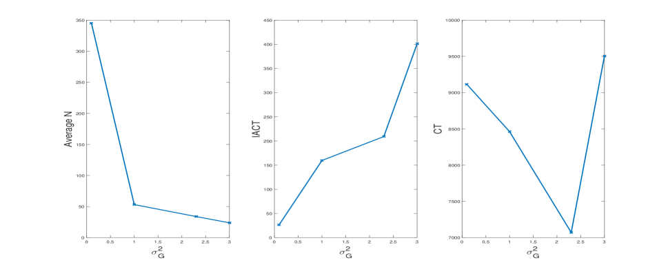
Figure 1: Panel-data example: Average $N_{i}$ ($\bar{N}$), IACT and CT = $\bar{N}\times$ IACT for various target $\sigma_{G}^{2}$, using MC.

We now report results using RQMC to estimate the likelihood, using the scrambled net algorithm of Matousek, (1998). We note that if $L_{i}(\theta)$ is estimated using RQMC, then the generated scrambled quasi random numbers are dependent although the estimate $\widehat{L}_{i}(\theta)$ is still unbiased. Thus, unlike MC, it is difficult to obtain a closed form expression for an unbiased estimator of the variance of $\widehat{L}_{i}(\theta)$. We therefore use replication to estimate each ${\mathbb{V}}(\log\widehat{L}_{i}(\bar{\theta}))$. Figure 2 shows that CT is minimised at $\sigma^{2}_{G}\approx 0.3$, which agrees with the theory in Lemma 3. CT increases slowly when $\sigma^{2}_{G}$ is smaller 0.3, but it increases quickly when $\sigma^{2}_{G}$ is higher than this value.

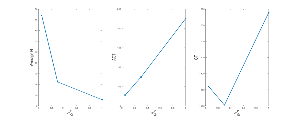
Figure 2: Panel-data example: Average $N_{i}$ ($\bar{N}$), IACT and CT = $\bar{N}\times$ IACT for various $\sigma_{G}^{2}$, using RQMC.

4.1.2 MC vs RQMC

We now compare the performance of the various schemes, and for simplicity use the same number of samples $N$ in all methods. We consider four schemes: independent PM using MC (IPM-MC), correlated PM using MC (CPM-MC), block PM using MC (BPM-MC), and block PM using RQMC (BPM-RQMC). We set $N_{i}=50$ across all $\theta$ and $i$, and verified that this was enough for both CPM and BPM chains to converge. The IPM-MC chain is unlikely to converge in this setting, as it requires a much larger $N$.

Table 2 summarises the performance measures using the BPM-RQMC as the baseline. The two block PM frameworks outperform both IPM-MC and CPM-MC. BPM-MC is somewhat faster than BPM-RQMC, but BPM-RQMC is much more efficient and has three times lower TNV compared to BPM-MC.

Methods	Acceptance rate	IACT ratio	CPU ratio	TNV ratio
IPM-MC	0.002	12.005	1.124	13.493
CPM-MC	0.081	5.273	1.133	5.974
BPM-MC	0.179	4.121	0.742	3.057
BPM-RQMC	0.225	1	1	1

Table 2: Panel-data example: comparison of independent PM using MC, block PM using MC, and block PM using RQMC. The BPM-RQMC is used as the baseline.

4.2 Data subsampling example

Quiroz et al., 2016c propose a data subsampling approach to Bayesian inference to speed up MCMC when the likelihood can be computed. The subsampling approach expresses the log-likelihood as a sum of terms and estimates it unbiasedly by summing a sample of the terms using control variates and simple random sampling. The unbiased log-likelihood estimator is converted to a slightly biased likelihood estimator in Quiroz et al., 2016c such that the PM targets a slightly perturbed target posterior. See also Quiroz et al., 2016a for an alternative unbiased estimator. Quiroz et al., 2016c use both the correlated PM and the block PM to carry out the estimation. For the block PM, $N_{(k)}=N_{k}=T/G$.

We illustrate the subsampling approach of Quiroz et al., 2016c and compare the block PM to the correlated PM using the following two $\mathrm{AR}(1)$ models with Student-t iid errors $\epsilon_{t}\sim t(\nu)$ with known degrees of freedom $\nu$. These examples are also used in their paper. The two models are ${\rm M}_{1}:\enspace y_{t}=\beta_{0}+\beta_{1}y_{t-1}+\epsilon_{t},q$ with $\theta=(\beta_{0}=0.3,\beta_{1}=0.6)$ and ${\rm M}_{2}:\enspace y_{t}=\mu+\rho(y_{t-1}-\mu)+\epsilon_{t}$, with $\theta=(\mu=0.3,\rho=0.99)$, for $t=1,...,T$, where $p(\epsilon_{t})\propto(1+\epsilon_{t}^{2}/\nu)^{-(\nu+1)/2}$ with $\nu=5$. Our aim is not to compare the two models, but to investigate the behaviour of BPM and CPM when data are generated from respective model. We use the same priors as in Quiroz et al., 2016c : $M_{1}:p(\beta_{0},\beta_{1})=\mathcal{U}(-5,5)\cdot\mathcal{U}(0,1)\quad\text{and}\quad M_{2}:p(\mu,\rho)=\mathcal{U}(-5,5)\cdot\mathcal{U}(0,1)$, where $\mathcal{U}(a,b)$ means a uniform density on the interval $(a,b)$.

Define $\ell_{t}(\theta):=\log p(y_{t}|y_{t-1},\theta)$ and rewrite the log-likelihood $\ell(\theta)$ as

$$\ell(\theta) =q(\theta)+d(\theta),\quad q(\theta)=\sum_{t=1}^{T}q_{t}(\theta),\quad d(\theta)=\sum_{t=1}^{T}d_{t}(\theta),\text{ with }d_{t}(\theta)=\ell_{t}(\theta)-q_{t}(\theta),$$

where $q_{t}(\theta)\approx\ell_{t}(\theta)$ is a control variate. We take $q_{t}(\theta)$ as a second order Taylor series approximation of $l_{t}(\theta)$ evaluated at the nearest centroid from a clustering in data space. This reduces the complexity of computing $q(\theta)$ from $O(T)$ to $O(C)$, where $C$ is the number of centroids. See Quiroz et al., 2016c for the details. An unbiased estimate of $\ell(\theta)$ based on a simple random sample with replacement is

$$\widehat{\ell}(\theta) =\widehat{d}(\theta)+q(\theta),$$ (9)

where

$$\widehat{d}(\theta)=\frac{T}{N}\sum_{i=1}^{N}d_{u_{i}}(\theta),\quad\text{with }\;u_{i}\in\{1,\dots,T\},\;\;{\rm P}(u_{i}=t)=\frac{1}{T},\quad t=1,\dots,T.$$

Here $N$ is the subsample size and $u=(u_{1},...,u_{N})$ represents a vector of observation indices. Write $\widehat{d}(\theta)$ as a sum of $G$ blocks

$$\widehat{d}=\widehat{d}^{(1)}+\cdots+\widehat{d}^{(G)},\quad\text{with}\quad\widehat{d}^{(k)}=\frac{T}{N}\sum_{i\in\mathcal{I}_{k}}d_{u_{i}},$$

where $\mathcal{I}_{k}$ with $|\mathcal{I}_{k}|=N_{(k)}$ contains the indices of the auxiliary variables corresponding to the $k$th block. We assume that the $N_{(k)}$ are the same for all $k$ and $N=G\times N_{(k)}$. Let $\sigma^{2}(\theta)={\mathbb{V}}(\widehat{l}(\theta))=(T/N)\sum_{t=1}^{T}(d_{i}(\theta)-\bar{d}(\theta))^{2}$ with $\bar{d}(\theta)=\sum d_{i}(\theta)/T$. Notice that $\mathbb{E}[\widehat{d}^{(k)}]=d(\theta)/{G}$ and ${\mathbb{V}}[\widehat{d}^{(k)}]={\sigma^{2}}/{G}$. Using the result that if $\widehat{d}\sim\mathcal{N}(d,\sigma^{2}/2)$, we have that $\mathbb{E}[\exp(q(\theta)+\widehat{d}(\theta)-\sigma^{2}(\theta)/2)]=\exp(l(\theta))$, Quiroz et al., 2016c work with the likelihood estimate

$$\widehat{L}(\theta,u) =\exp(q(\theta))\exp\left(\widehat{d(\theta)}-\frac{\widehat{\sigma}^{2}(\theta)}{2}\right)=\exp(q(\theta))\prod_{k=1}^{G}\exp\left(\widehat{d(\theta)}^{(k)}-\frac{\widehat{\sigma}^{2}(\theta)}{2G}\right),$$ (10)

where $\widehat{\sigma}^{2}(\theta)$ is an unbiased estimate of $\sigma^{2}(\theta)$, because computing $\sigma^{2}(\theta)$, to obtain an unbiased estimator of the likelihood, is expensive and defeats the purpose of subsampling. Quiroz et al., 2016c show that carrying out the PM with this slightly biased likelihood estimator samples from a perturbed posterior that is very close to the full-data posterior under quite general conditions.

We generated $T=100,000$ observations from the models in ${\rm M}_{1}$ and ${\rm M}_{2}$ and ran both the correlated PM and the block PM for $55,000$ iterations from which we discarded the first 5,000 draws as burn-in. Using the same target for $\sigma^{2}(\theta)$ as in Quiroz et al., 2016c results in sample sizes $N\approx 1300$ for model $M_{1}$ and $N\approx 2600$ for model $M_{2}$. For the block PM we use $G=100$. Also, following Quiroz et al., 2016c , the correlation parameter in the correlated PM is set to $\varrho=0.9999$, and we use a random walk proposal which is adapted during the burn-in phase to target an acceptance rate of approximately $0.15$ (Sherlock et al.,, 2015).

Table 3 summarises the performance measures introduced in Section 4.1. It is evident that the block PM significantly outperforms the correlated PM in terms of CPU time and TNV. This is because, as discussed above, the correlated PM requires $N$ operations for generating the vector $\bm{u}$. The block PM moves only one block at a time, so that the update of the vector $u$ requires $N/G$ operations.

Methods	Acceptance rate		IACT ratio		CPU ratio		TNV ratio
	$\mathrm{M}_{1}$	$\mathrm{M}_{2}$	$\mathrm{M}_{1}$	$\mathrm{M}_{2}$	$\mathrm{M}_{1}$	$\mathrm{M}_{2}$	$\mathrm{M}_{1}$	$\mathrm{M}_{2}$
CPM	0.149	0.140	1.110	1.124	62.893	38.610	69.444	43.478
BPM	0.160	0.151	1	1	1	1	1	1

Table 3: Data subsampling example using block PM as a baseline.

4.3 Diffusion process example

This section applies the PM approaches to estimate the parameters of the diffusion process $\bm{X}=\{X_{t},t\geq 0\}$ governed by the stochastic differential equation (SDE)

$$dX_{t}=\mu(X_{t},\theta)dt+\sigma(X_{t},\theta)dW_{t},$$ (11)

with $W_{t}$ a Wiener process. We assume that the regularity conditions on $\mu(\cdot,\cdot)$ and $\sigma(\cdot,\cdot)$ are met so that the solution to the SDE in (11) exists and is unique. We are interested in estimating the vector of parameters $\theta$ based on discrete-time observations $x=\{x_{0},x_{1},...,x_{n}\}$, where $x_{i}$ is the observation of $X_{i\Delta}$ with $\Delta$ some time-interval. The likelihood is

$$L(\theta):=p(x|\theta)=\prod_{i=0}^{n-1}p_{\Delta}(x_{i+1}|x_{i},\theta),$$

where the $\Delta$-interval Markov transition density $p_{\Delta}(x_{i+1}|x_{i},\theta)$ is typically intractable. In order to make the discrete approximation of the continuous-time process $X$ sufficiently accurate, we follow Stramer and Bognar, (2011) and write $p_{\Delta}(x_{i+1}|x_{i},\theta)$ as

$$p_{\Delta}(x_{i+1}|x_{i},\theta)=\int p_{h}(x_{i+1}|z_{i,M-1},\theta)p_{h}(z_{i,M-1}|z_{i,M-2},\theta)\cdots p_{h}(z_{i,1}|x_{i},\theta){\rm d}\,z_{i,1}\cdots{\rm d}\,z_{i,M-1},$$ (12)

where $p_{h}(\cdot|\cdot,\theta)$ is the Markov transition density of $X$ after time-step $h=\Delta/M$. The Euler approximation

$$p_{h}^{\text{euler}}(u|v,\theta)=\mathcal{N}\Big{(}u;v+h\mu(v,\theta),h\Sigma(v,\theta)\Big{)},$$

with $\Sigma(v,\theta)=\sigma(v,\theta)\sigma^{\prime}(v,\theta)$, is a very accurate approximation to $p_{h}(u|v,\theta)$ if $h$ is sufficiently small. We approximate the transition density in (12) by

$$p_{\Delta}^{\text{euler}}(x_{i+1}|x_{i},\theta)=\int p_{h}^{\text{euler}}(x_{i+1}|z_{i,M-1},\theta)p_{h}^{\text{euler}}(z_{i,M-1}|z_{i,M-2},\theta)\cdots p_{h}^{\text{euler}}(z_{i,1}|x_{i},\theta){\rm d}\,z_{i,1}\cdots{\rm d}\,z_{i,M-1},$$

and follow Stramer and Bognar, (2011) and define the working likelihood as

$$L^{\text{euler}}(\theta)=\prod_{i=0}^{n-1}p_{\Delta}^{\text{euler}}(x_{i+1}|x_{i},\theta).$$

The posterior density of $\theta$ is then $p^{\text{euler}}(\theta|x)\propto p_{\Theta}(\theta)L^{\text{euler}}(\theta).$ The likelihood $L^{\text{euler}}(\theta)$ is intractable, but can be estimated unbiasedly. As in Stramer and Bognar, (2011), we estimate $p_{\Delta}^{\text{euler}}(x_{i+1}|x_{i},\theta)$ using the importance sampler of Durham and Gallant, (2002),

$$z_{i,m+1}\sim\mathcal{N}\left(z_{i,m}+\frac{x_{i+1}-z_{i,m}}{M-m},h\frac{M-m-1}{M-m}\Sigma(z_{i,m},\theta)\right),\;\;m=0,...,M-2,$$

where $z_{i,0}=x_{i}$. The density of this importance distribution is

$$g(z_{i})=g(z_{i,1},...,z_{i,M-1})=\prod_{m=0}^{M-2}\mathcal{N}\left(z_{i,m+1};z_{i,m}+\frac{x_{i+1}-z_{i,m}}{M-m},h\frac{M-m-1}{M-m}\Sigma(z_{i,m},\theta)\right).$$

We sample $N$ such trajectories $z_{i}^{(j)}=(z_{i,1}^{(j)},...,z_{i,M-1}^{(j)})$, $j=1,...,N$ and denote by $\bm{u}_{i}$ the set of all required MC random numbers, $i=0,...,n-1$. Then, the unbiased estimator of $p_{\Delta}^{\text{euler}}(x_{i+1}|x_{i},\theta)$ is

$$\widehat{p}_{\Delta}^{\text{euler}}(x_{i+1}|u_{i},x_{i},\theta)=\frac{1}{N}\sum_{j=1}^{N}\frac{p_{h}^{\text{euler}}(x_{i+1}|z_{i,M-1}^{(j)},\theta)p_{h}^{\text{euler}}(z_{i,M-1}^{(j)}|z_{i,M-2}^{(j)},\theta)\cdots.p_{h}^{\text{euler}}(z_{i,1}^{(j)}|x_{i},\theta)}{g(z_{i}^{(j)})}$$

The working likelihood $L^{\text{euler}}(\theta)$ factorises as in (6) and is estimated unbiasedly, so all the theory developed in Sections 3 and B applies here as well.

We apply the proposed method to fit the FedFunds dataset to the Cox-Ingersoll-Ross (CIR) model

$$dX_{t}=\beta(\alpha-X_{t})dt+\sigma\sqrt{X_{t}}dW_{t},$$

using MC pseudo random numbers. The FedFunds dataset we use consists of 745 monthly federal funds rates in the US from July 1954 to August 2016, downloaded from Yahoo Finance (https://au.finance.yahoo.com/).

We follow Stramer and Bognar, (2011) and set $\Delta=1/12$ and also use the prior

$$p_{\Theta}(\theta)=I_{(0,1)}(\alpha)I_{(0,\infty)}(\beta)\sigma^{-1}I_{(0,\infty)}(\sigma)$$

where $I_{(a,b)}(x)=1$ if $x\in(a,b)$ and 0 otherwise.

We take $M=300$ to make the Euler approximation highly accurate, Stramer and Bognar, (2011) use $M=20$. We use $N=1$ samples and $G=186$ groups so that $u_{(k)}=\{u_{3(k-1)},u_{3(k-1)+1},u_{3(k-1)+2}\}$, $k=1,...,G$. Table 4 summarises the results, which show that the block PM performs better than the independent PM. Stramer and Bognar, (2011) report that their blocking strategy does not work better than the independent PM. There are three reasons for this different conclusion. First, Stramer and Bognar,’s dataset consists of 432 monthly rates from January 1963 to December 1998, which is a little over half of our dataset. Second, they set $M=20$ and $N=5$ while we set $M=300$ and $N=1$. For both these reasons, the estimate of the log likelihood in their problem has a variance that is small and less than 1 and hence our theory predicts that the independent PM will be as good as the block PM, and shows the value of our theoretical guidelines. The variance of the log of the likelihood estimate in our setting is much greater than 1 so that our setting is much more challenging for the independent PM because the estimates of the likelihood are highly variable. Third, Stramer and Bognar, (2011) use a MCMC scheme that treats $\theta$ and the $G$ blocks ${{\bm{u}}}_{(1)}$,…,${{\bm{u}}}_{(G)}$ as $G+1$ blocks that are generated one at a time conditional on all the other blocks. Our MCMC scheme updates $\theta$ and one of the ${{\bm{u}}}_{(i)}$ jointly in each iteration.

Methods	Acceptance rate	IACT ratio	CPU ratio	TNV ratio
IPM	0.049	9.059	1.154	10.45
BPM	0.258	1	1	1

Table 4: Diffusion process example: Comparing the independent PM (IPM) and the block PM (BPM) using the block PM as the baseline.

5 Conclusion

Deligiannidis et al., (2016) show how the PM approach can be made much more efficient by correlating the underlying Monte Carlo (MC) random numbers used to form the estimate of the likelihood at the current and proposed values of the unknown parameters. Their approach greatly speeds up the standard PM algorithm, as it requires a much smaller number of samples or particles to form the optimal likelihood estimate. Our paper presents an alternative implementation of the correlated PM approach, called the block PM, which divides the underlying random numbers into blocks so that the likelihood estimates for the proposed and current values of the parameters only differ by the random numbers in one block. We show that this implementation of the correlated PM can be much more efficient for some specific problems than the implementation in Deligiannidis et al., (2016); for example when the likelihood is estimated by subsampling or the likelihood is a product of terms each of which is given by an integral which can be estimated unbiasedly by randomised quasi-Monte Carlo. Using stylized but realistic assumptions the article also provides methods and guidelines for implementing the block PM efficiently. As already discussed, we have successfully implemented the block PM in several applications and shown that it results in greatly improved performance of the PM sampler. A second advantage of the the block PM is that it provides a direct way to control the correlation between the logarithms of the estimates of the likelihood at the current and proposed values of the parameters than the implementation in Deligiannidis et al., (2016). We obtain methods and guidelines for selecting the optimal number of samples based on idealized but realistic assumptions. Finally, we believe that in future applications CPM can be combined with BPM to produce efficient PM algorithms.

Online Supplement to ‘The Block Pseudo-Marginal Sampler’

Appendix A Proofs

Proof of Lemma 1.

We will show that

$$\left(\prod_{i=1}^{G}p_{{{\bm{U}}}_{(i)}}({{\bm{u}}}_{(i)})\right)q({\rm d}\,{{\bm{u}}}_{(1:G)}^{\prime}|{{\bm{u}}}_{(1:G)}) =\left(\prod_{i=1}^{G}p_{{{\bm{U}}}_{(i)}}({{\bm{u}}}_{(i)}^{\prime})\right)q({\rm d}\,{{\bm{u}}}_{(1:G)}|{{\bm{u}}}_{(1:G)}^{\prime})$$ (S1)

Define the measure

$$\nu_{j}({\rm d}\,\bm{u}_{(1:G)},{\rm d}\,\bm{u}^{\prime}_{(1:G)}):=p_{U_{(j)}}(\bm{u}_{(j)}){\rm d}\,\bm{u}_{(j)}\prod_{k\neq j}\left(\delta_{\bm{u}^{\prime}_{(k)}}({\rm d}\,\bm{u}_{(k)})p_{U_{(k)}}(\bm{u}_{(k)}){\rm d}\,\bm{u}_{(k)}.\right)$$

It is straightforward to show that $\nu_{j}({\rm d}\,\bm{u}_{(1:G)},{\rm d}\,\bm{u}^{\prime}_{(1:G)})=\nu_{j}({\rm d}\,\bm{u}^{\prime}_{(1:G)},{\rm d}\,\bm{u}_{(1:G)})$ by showing that for any integrable function $h(\bm{u}_{(1:G)},\bm{u}^{\prime}_{(1:G)})$ with respect to $\nu_{j}({\rm d}\,\bm{u}_{(1:G)},{\rm d}\,\bm{u}^{\prime}_{(1:G)})$ we will have that

$$\int h(\bm{u}_{(1:G)},\bm{u}^{\prime}_{(1:G)})\nu_{j}({\rm d}\,\bm{u}_{(1:G)},{\rm d}\,\bm{u}^{\prime}_{(1:G)})=\int h(\bm{u}_{(1:G)},\bm{u}^{\prime}_{(1:G)})\nu_{j}({\rm d}\,\bm{u}^{\prime}_{(1:G)},{\rm d}\,\bm{u}_{(1:G)}).$$

The result of the lemma now follows. ∎

It is useful to have the following definitions and results to obtain Lemmas 2 and 3. For any $\theta\in\Theta$, ${{\bm{u}}}_{(i)}\in\mathbb{U}_{i}$, $i=1,\dots,G$, we define ${{z}}_{(k)}$, $z(\theta,{{\bm{u}}}_{(1:G)})$ and $z(\theta,{{\bm{u}}}_{(i_{1}:i_{k})})$ as in Section 3.1, and $\mathcal{Z}(\theta,{{\bm{u}}}_{(1:G)}):=\left({{z}}_{(1)}(\theta,{{\bm{u}}}_{(1)}),\dots,{{z}}_{(G)}(\theta,{{\bm{u}}}_{(G)})\right)^{\rm T}$.

For $j=1,\dots,G$, let ${{g}}_{(j)}({{z}}_{(j)}|\theta)$ be the density of ${{z}}_{(j)}$ when ${{\bm{u}}}_{(j)}$ has density $p_{{{\bm{U}}}_{(j)}}(\cdot)$, and let $g_{Z}(z|\theta)$ be the corresponding density of $z$. The following lemma is a straightforward generalization of the approach in Pitt et al., (2012).

Lemma S1.

If the ${{\bm{u}}}_{(j)}$ are independent, each with density $p_{{{\bm{U}}}_{(j)}}(\cdot)$, for $j=1,\dots,G$, then

1. $\int\exp({{z}}_{(j)}){{g}}_{(j)}({{z}}_{(j)}|\theta){\rm d}\,{{z}}_{(j)}=1\quad\text{and}\quad\int\exp(z)g_{Z}(z|\theta){\rm d}\,z=1.$

2. $\overline{\pi}(\theta,{{\bm{u}}}_{(1)},\dots,{{\bm{u}}}_{(G)})=\prod_{j=1}^{G}\exp(z(\theta,{{\bm{u}}}_{(j)}))p_{{{\bm{U}}}_{(j)}}({{\bm{u}}}_{(j)})\pi(\theta),$ so that

   $$\overline{\pi}({{\bm{u}}}_{(1:G)}|\theta)=\prod_{j=1}^{G}\exp(z(\theta,{{\bm{u}}}_{(j)}))p_{{{\bm{U}}}_{(j)}}({{\bm{u}}}_{(j)}).$$

   Hence, conditional on $\theta$, the ${{\bm{u}}}_{(j)}$ are independent in the posterior and have densities $\exp(z(\theta,{{\bm{u}}}_{(j)}))p_{{{\bm{U}}}_{(j)}}({{\bm{u}}}_{(j)})$.

3. $\overline{\pi}({{z}}_{(1)},\dots,{{z}}_{(G)}|\theta)=\prod_{j=1}^{G}\exp({{z}}_{(j)}){{g}}_{(j)}({{z}}_{(j)}|\theta)$ so that, conditional on $\theta$, $z_{(1)},\dots,z_{(G)}$ are independent in the posterior with $z_{(j)}$ having density $\exp({{z}}_{(j)}){{g}}_{(j)}({{z}}_{(j)}|\theta)$.

4. $\overline{\pi}(z|\theta)=\exp(z)g_{Z}(z|\theta)$ so that $\overline{\pi}(z,\theta)=\overline{\pi}(z|\theta)\pi(\theta)$.

Pseudo-marginal MCMC based on $\mathcal{Z}$

Consider now the hypothetical pseudo-marginal MCMC sampling scheme on $\mathcal{Z}$ with block proposal density for $\mathcal{Z}$, conditional on $\theta$, given by

$$q_{Z}(\mathcal{Z}|\mathcal{Z}^{\prime},\theta):=\sum_{i=1}^{G}\omega_{i}g_{i}({{z}}_{(i)}|\theta)\prod_{j\neq i}\delta_{{{z}}_{(j)}^{\prime}}({\rm d}\,{{z}}_{(j)})$$ (S2)

with $\omega_{i}=1/G$. The proposal for $\theta$ is as above. Lemma S2 below shows that studying the optimality properties of the PM simulation based on $\theta$ and $\bm{u}$ is equivalent to studying it for $\theta$ and $\mathcal{Z}$. Although the PM based on the $\mathcal{Z}$ is only ‘hypothetical’, as we usually cannot compute it, we show below that it is more convenient to work with $\mathcal{Z}$.

Lemma S2.

1. The acceptance probability (5) can be written as

   $$\min\left\{1,\exp\left(z(\theta,{{\bm{u}}}_{(1:k-1)}^{\prime},{{\bm{u}}}_{(k)},{{\bm{u}}}_{(k+1:G)}^{\prime})-z(\theta^{\prime},{{\bm{u}}}_{(1:G)}^{\prime})\right)\frac{\pi(\theta)}{\pi(\theta^{\prime})}\frac{q_{\Theta}(\theta^{\prime}|\theta)}{q_{\Theta}(\theta|\theta^{\prime})}\right\}$$ (S3)

2. The acceptance probability of a PM scheme based on $\mathcal{Z}$ with proposal (S2) is equal to (S3). Under Assumption 3, it becomes $\min\left\{1,\exp(z-z^{\prime})\right\}.$

The following lemma and corollary are needed to prove Lemma 2. Their proofs are straightforward and omitted.

Lemma S3.

Suppose that Assumption 1 holds. Then,

1. If the ${{\bm{u}}}_{(k)}$ are independent and generated from $p_{{{\bm{U}}}_{(k)}}(\cdot)$ for $k=1,\dots,G$, then $z(\theta,{{\bm{u}}}_{(1:G)})\sim\mathcal{N}(-\sigma^{2}/2,\sigma^{2})$ and $z(\theta,{{\bm{u}}}_{(1:k-1)},{{\bm{u}}}_{(k+1:G)})\sim\mathcal{N}(-((G-1)/2G)\sigma^{2},((G-1)/G)\sigma^{2})$.

2. $\overline{\pi}(z(\theta,{{\bm{u}}}_{(1:G)})|\theta))=\mathcal{N}(z;\sigma^{2}/2,\sigma^{2})$ and $\overline{\pi}(z(\theta,{{\bm{u}}}_{(1:k-1)},{{\bm{u}}}_{(k+1:G)})|\theta)=\mathcal{N}(z;((G-1)/2G)\sigma^{2},((G-1)/G)\sigma^{2})$.

Corollary S1.

Suppose that Assumptions 1 and 2 hold. If $({{\bm{u}}}_{(1:k-1)}^{\prime},{{\bm{u}}}_{(k+1:G)}^{\prime})\sim\overline{\pi}(\cdot|\theta)$ and ${{\bm{u}}}_{(k)}\sim p_{{{\bm{U}}}_{(k)}}(\cdot)$ and they are independent, then, ${{z}}_{(k)}(\theta,{{\bm{u}}}_{(k)})+z(\theta,{{\bm{u}}}_{(1:k-1)}^{\prime},{{\bm{u}}}_{(k+1:G)}^{\prime})\sim\mathcal{N}(((G-2)/2G)\sigma^{2},\sigma^{2})$.

Proof of Lemma 2.

The proof of the lemma follows directly from Lemma S3 and Corollary S1. ∎

The next lemma gives the conditional and unconditional acceptance probabilities of the Metropolis-Hastings scheme for $z$ and $\theta$.

Lemma S4.

Suppose Assumptions 1 to 3 hold and $\rho=1-1/G$.

• The acceptance probability of the Metropolis-Hastings scheme conditional on $z^{\prime}:=z(\theta^{\prime},{{\bm{u}}}_{(1:G)}^{\prime})$ is

  $${\rm P}({\rm accept}|z^{\prime},\rho,\sigma) =\exp(-x+\tau^{2}/2)\Phi\left(\frac{x}{\tau}-\tau\right)+\Phi\left(\frac{-x}{\tau}\right)$$

  with $x:=\bigg{(}z^{\prime}+\frac{\sigma^{2}}{2}\bigg{)}(1-\rho)$ and $\tau:=\sigma\sqrt{1-\rho^{2}}$.

• The unconditional acceptance probability of the Metropolis-Hastings scheme is

  $${\rm P}({\rm accept}|\rho,\sigma)=2\left(1-\Phi\Big{(}\frac{\sigma\sqrt{1-\rho}}{\sqrt{2}}\Big{)}\right).$$ (S4)

Proof.

We use the following results to obtain the conditional acceptance probability.

$$\int_{-\infty}^{A}\exp(z)\mathcal{N}(z;a,b^{2})dz =\exp(a+b^{2}/2)\Phi\bigg{(}\frac{A-a-b^{2}}{b}\bigg{)}$$ (S5)

$$\int_{A}^{\infty}\mathcal{N}(z;a,b^{2})dz =\Phi\bigg{(}\frac{a-A}{b}\bigg{)},\$$ (S6)

where $\Phi(\cdot)$ denotes the standard normal CDF. From Lemma 2, we have that $a(z^{\prime}):=\mathbb{E}(z|z^{\prime})=-\sigma^{2}/2G+\rho z^{\prime}$ and $\tau^{2}:={\mathbb{V}}(z|z^{\prime})=\sigma^{2}(1-\rho^{2})$, so that the conditional density of $z$ given $z^{\prime}$ is $\mathcal{N}(z;a(z^{\prime}),\tau^{2})$. Using (S5) and (S6), the conditional probability of acceptance is

$$\int\min(1,\exp(z-z^{\prime})) \mathcal{N}(z;a(z^{\prime}),\tau^{2}){\rm d}\,z=\int_{-\infty}^{z^{\prime}}\exp(z-z^{\prime})\mathcal{N}(z;a(z^{\prime}),\tau^{2})dz+\int_{z^{\prime}}^{\infty}\mathcal{N}(z;a(z^{\prime}),\tau^{2}){\rm d}\,z$$

$$=\exp\bigg{(}a(z^{\prime})-z^{\prime}+\tau^{2}/2\bigg{)}\Phi\bigg{(}\frac{z^{\prime}-a(z^{\prime})-\tau^{2}}{\tau}\bigg{)}+\Phi\bigg{(}\frac{a(z^{\prime})-z^{\prime}}{\tau}\bigg{)}$$

$$=\exp\bigg{(}-y+\tau^{2}/2\bigg{)}\Phi\bigg{(}\frac{y-\tau^{2}}{\tau}\bigg{)}+\Phi\bigg{(}\frac{-y}{\tau}\bigg{)},$$

where $y:=z^{\prime}-a(z^{\prime})=(1-\rho)(z^{\prime}+\sigma^{2}/2)$.

We now obtain the unconditional acceptance probability. We deduce from Lemma 2 that $z-z^{\prime}\sim\mathcal{N}(-\sigma^{2}(1-\rho);2\sigma^{2}(1-\rho))$. The required result is now obtained using the identity $e^{v}\mathcal{N}(v;-a,2a)=\mathcal{N}(v;a,2a)$, with $a=\sigma^{2}(1-\rho)$. ∎

We use the next lemma to prove Lemma 3. It is of interest in its own right as it shows that under our assumptions the inefficiency is independent of the function.

Lemma S5.

The inefficiency is given by

$$\text{\rm IF}(\sigma,\rho)=1+2\mathbb{E}_{z^{\prime}\sim\pi(z^{\prime}|\sigma)}\bigg{(}\frac{1-k(z^{\prime}|\sigma,\rho)}{k(z^{\prime}|\sigma,\rho)}\bigg{)},$$ (S7)

where $k(z^{\prime}|\rho,\sigma)=\Pr({\rm accept}|z^{\prime},\rho,\sigma)$ is the acceptance probability of the MCMC scheme conditional on the previous iterate $z^{\prime}$ and is given by part (i) of Lemma S4.

Proof.

For notational simplicity, we write the proposal density $q(z|z^{\prime};\rho,\sigma)$ as $q(z|z^{\prime})$, the acceptance probability $\min\left\{1,\exp(z-z^{\prime})\right\}.$ as $\alpha(z^{\prime},z;\rho,\sigma)$ as $\alpha(z^{\prime},z)$ and the acceptance probability $k(z^{\prime}|\sigma,\rho)$, conditional on the previous iterate, as $k(z^{\prime})$. Let $\{(\theta^{[j]},z^{[j]}),j=1,\dots,M\}$ be iterates, after convergence, of the Markov chain produced by the PM sampling scheme. Then, the Markov transition distribution from $(\theta^{\prime},z^{\prime})$ to $(\theta,z)$ is

$$p(\theta^{\prime},z^{\prime};{\rm d}\,\theta,{\rm d}\,z) = \alpha(z^{\prime},z)\pi(\theta)q(z|z^{\prime}){\rm d}\,\theta{\rm d}\,z+\left(1-\int\alpha(z^{\prime},z^{*})\pi(\theta^{*})q(z^{*}|z^{\prime})d\theta^{*}dz^{*}\right)\delta_{(\theta^{\prime},z^{\prime})}({\rm d}\,\theta,{\rm d}\,z)$$

$$= \alpha(z^{\prime},z)\pi(\theta)q(z|z^{\prime})d\theta dz+\left(1-k(z^{\prime}|\sigma,\rho)\right)\delta_{(\theta^{\prime},z^{\prime})}(d\theta,dz),$$

$\delta_{\theta^{\prime},z^{\prime}}({\rm d}\,\theta,{\rm d}\,z)$ is the probability measure concentrated at $(\theta^{\prime},z^{\prime})$.

Consider now the space of functions

$$\mathfrak{F}=\bigg{\{}\widetilde{\varphi}:\widetilde{\Theta}=\Theta\otimes\mathbb{R}\mapsto\mathbb{R} ,\widetilde{\varphi}=\varphi(\theta)\psi(z),\pi(\varphi):=\mathbb{E}_{\theta\sim\pi(\theta)}(\varphi)=0,\pi(\varphi^{2}):=\mathbb{E}_{\theta\sim\pi(\theta)}(\varphi^{2})<\infty,$$

$$\pi(\psi^{2}):=E_{z\sim\pi(z)}(\psi)^{2}<\infty\bigg{\}}.$$

We define the operator $P:\mathfrak{F}\mapsto\mathfrak{F}$ as

$$(P\widetilde{\varphi})(\theta,z) :=\int\widetilde{\varphi}(\theta^{*},z^{*})p(\theta,z;\theta^{*},z^{*})d\theta^{*}dz^{*}$$

$$=\pi(\varphi)\int\psi(z)\alpha(z,z^{*})q(z^{*}|z)dz^{*}+\widetilde{\varphi}(\theta)(1-k(z))$$

$$=\varphi(\theta)\psi(z)(1-k(z)).$$

as $\pi(\varphi)=0$ by assumption. It is straightforward to check that $(P^{j}\widetilde{\varphi})(\theta,z)=\varphi(\theta)\psi(z)(1-k(z))^{j}$ and that $(P\widetilde{\varphi})(\theta^{[j-1]},z^{[j-1]})=E(\widetilde{\varphi}(\theta^{[j]},z^{[j]})|\theta^{[j-1]},z^{[j-1]})$. Hence, $(P^{j}\varphi)(\theta_{0},z_{0})=\widetilde{\varphi}(\theta_{0},z_{0})(1-k(z_{0}))^{j}$.

We now consider $\widetilde{\varphi}(\theta,z)=\varphi(\theta)\psi(z)$ with $\psi(z)\equiv 1$ so that $\widetilde{\varphi}\in\mathfrak{F}$; suppose also that $(\theta_{0},z_{0})\sim\widetilde{\pi}_{N}$. Define $c_{j}:={\rm Cov}(\widetilde{\varphi}(\theta^{[j]},z^{[j]}),\widetilde{\varphi}(\theta^{[0]},z^{[0]}))={\rm Cov}(\varphi(\theta^{[j]}),\varphi(\theta^{[0]}))$. Then,

$$c_{j} =\mathbb{E}\big{(}\widetilde{\varphi}(\theta^{[0]},z^{[j]})\widetilde{\varphi}(\theta^{[0]},z^{[0]})\big{)}$$

$$=\mathbb{E}_{(\theta^{[0]},z^{[0]})\sim\widetilde{\pi}_{N}}\big{(}\mathbb{E}(\widetilde{\varphi}(\theta^{[0]},z^{[j]})|\theta^{[0]},z^{[0]})\widetilde{\varphi}(\theta^{[0]},z^{[0]})\big{)}$$

$$=\mathbb{E}_{(\theta^{[0]},z^{[0]})\sim\widetilde{\pi}_{N}}\big{(}(1-k(z_{0}))^{j}\widetilde{\varphi}(\theta^{[0]},z^{[0]})^{2}\big{)}$$

$$=\mathbb{E}_{z^{[0]}\sim\widetilde{\pi}_{N}(z)}\big{(}(1-k(z^{[0]}))^{j})\mathbb{E}_{\theta^{[0]}\sim\pi}(\varphi(\theta^{[0]})^{2}\big{)}$$

because $$z^{[0]} \sigma$$ only depends on by construction

$$=\mathbb{E}_{z^{[0]}\sim\widetilde{\pi}_{N}(z)}\big{(}(1-k(z^{[0]}))^{j}\big{)}c_{0}.$$

The inefficiency IF is defined as

IF $$=(c_{0}+2\sum_{j=1}^{\infty}c_{j})/c_{0}=1+2\sum_{j=1}^{\infty}\mathbb{E}_{z\sim\widetilde{\pi}_{N}(z)}\bigg{(}\big{(}1-k(z)\big{)}^{j}\bigg{)}=1+2\mathbb{E}_{z\sim\widetilde{\pi}_{N}(z)}\bigg{(}\frac{1-k(z)}{k(z)}\bigg{)}$$

as required. ∎

Proof of Lemma 3.

From Lemma 2, $\overline{\pi}(z^{\prime}|\sigma)=\mathcal{N}(z^{\prime};\sigma^{2}/2,\sigma^{2})$. Let $\omega:=[(1-\rho)(z^{\prime}+\sigma^{2}/2)-\tau^{2}]/\tau$ with $\tau=\sigma\sqrt{1-\rho^{2}}$. Then,

$$\omega \sim\mathcal{N}\bigg{(}-\frac{\rho\tau}{1+\rho},\frac{1-\rho}{1+\rho}\bigg{)},$$

and we note that the variance of $\omega$ just depends on $\rho$. For $\rho$ close to 1, the variance of $\omega$ is approximately $1/(2G)$, which is very small. Thus, $\omega$ will be concentrated close to its mean $\omega^{*}:=-\rho\tau/(1+\rho)$. Define $p^{*}(\omega|\tau):=1-k(z^{\prime}|\rho,\sigma)=\Phi(\omega+\tau)+\exp(-\omega\tau-\tau^{2}/2)\Phi(\omega)$. Then,

$$\text{\rm IF}(\sigma,\rho) =\int\frac{1+p^{*}(\omega|\tau)}{1-p^{*}(\omega|\tau)}\mathcal{N}\bigg{(}\omega;-\frac{\rho\tau}{1+\rho},\frac{1-\rho}{1+\rho}\bigg{)}d\omega.$$

It is convenient to write $\text{\rm IF}(\sigma,\rho)$ as $\text{\rm IF}(\tau|\rho)$, which we will optimize the computing time over $\tau$ keeping $\rho$ fixed. Let,

$$f(\omega;\tau) :=\frac{1+p^{*}(\omega|\tau)}{1-p^{*}(\omega|\tau)}.$$

Using the 4th order Taylor series expansion of $f(w;\tau)$ at $\omega=\omega^{*}$, the inefficiency factor can be approximated by

$$\text{\rm IF}_{\rm approx}(\tau|\rho)=f(\omega^{*}|\tau)+\frac{1}{2}\frac{1-\rho}{1+\rho}f^{(2)}(\omega^{*}|\tau)+\frac{1}{8}\left(\frac{1-\rho}{1+\rho}\right)^{2}f^{(4)}(\omega^{*}|\tau),$$

which is considered as a function of $\tau$ with $\rho$ fixed. This approximation is very accurate because, as noted, the variance of $\omega$ is very small for large $G$. So the computing time $\text{\rm CT}(\sigma,\rho)={\text{\rm IF}(\sigma,\rho)}/{\sigma^{1/\varpi}}$ is approximated by

$$\text{\rm CT}_{\rm approx}(\tau|\rho) =(1-\rho^{2})^{\frac{1}{2\varpi}}\frac{\text{\rm IF}_{\rm approx}(\tau|\rho)}{\tau^{1/\varpi}}\propto\frac{\text{\rm IF}_{\rm approx}(\tau|\rho)}{\tau^{1/\varpi}}$$

Minimizing this term over $\tau$, for $\rho$ close to 1, we find that $\text{\rm CT}_{\rm approx}(\tau|\rho)$ is minimized at $\tau\approx 2.16$ for $\varpi=1/2$, and at $\tau\approx 0.82$ for $\varpi\approx 3/2$. So the optimal $\sigma_{\text{\rm opt}}\approx 2.16/\sqrt{1-\rho^{2}}$ for $\varpi=1/2$ and $\sigma_{\text{\rm opt}}\approx 0.82/\sqrt{1-\rho^{2}}$ for $\varpi=3/2-\epsilon$ with any arbitrarily small $\epsilon$.

For $\sigma_{\text{\rm opt}}\approx 2.16/\sqrt{1-\rho^{2}}$, the unconditional acceptance rate (S4) is

$$P(\text{accept}|\rho,\sigma_{\text{\rm opt}}) = 2\left(1-\Phi\Big{(}\frac{\sigma_{\text{\rm opt}}\sqrt{1-\rho}}{\sqrt{2}}\Big{)}\right)$$

$$= 2\left(1-\Phi\Big{(}\frac{\sigma_{\text{\rm opt}}\sqrt{1-\rho^{2}}}{\sqrt{2(1+\rho)}}\Big{)}\right)$$

$$\approx 2\left(1-\Phi\Big{(}\frac{2.16}{{2}}\Big{)}\right)\approx 0.28.$$

Similarly, for $\sigma_{\text{\rm opt}}\approx 0.82/\sqrt{1-\rho^{2}}$, this probability is approximately 0.68. ∎

Appendix B Some large-sample properties of block PM for panel-data

This section derives some properties of the block PM for large $T$ for the panel-data models discussed in Sections 3 and 4.1 and shows that: (a) the total number of samples required per MCMC iteration is $O(T^{3/2})$ if MC is used; and $O(T^{7/6})$ if RQMC is used, whereas the independent PM requires $O(T^{2})$ samples; and (b) we show that when $T$ is large the posterior correlation between $\theta$ and $z$ is weak. Since $\pi(\theta,z)$ is asymptotically (in $T$) multivariate normal, this means that $\theta$ and $z$ are close to independent when $T$ is large, suggesting that moving $\bm{u}$ slowly, and hence moving $z$ slowly for a given $\theta$, does not greatly affect the mixing of the $\theta$ iterates.

Consider the panel-data model, with the panels in the $k$th block denoted by ${\cal G}_{k}$, and suppose that we use the same $N_{i}=N_{k}$ samples for all panels $i\in{\cal G}_{k}$. Let $L_{i}(\theta)=p(y_{i}|\theta)$ be the likelihood of the $i$th panel, and let $\widehat{L}_{i}(\theta,\bm{u}_{i})$ be the unbiased estimate of $L_{i}(\theta)$. We assume that

Assumption S4.

For each $i\in{\cal G}_{k}$ and parameter value $\theta$, there exists an $A_{i}(\theta)^{2}$ such that as $N_{k}\rightarrow\infty$,

$$N_{k}^{\varpi}\bigg{(}\widehat{L}_{i}(\theta,u_{i})-L_{i}(\theta)\bigg{)} \stackrel{{\scriptstyle d}}{{\Rightarrow}}\mathcal{N}(0,A_{i}(\theta)^{2}),$$ (S8)

for some $\varpi>0$.

The central limit theorem (S8) holds for most importance sampling estimates of the likelihood, where $\varpi=1/2$ if MC is used and $\varpi=3/2-\epsilon$, with an arbitrarily small $\epsilon>0$, if RQMC is used (see, e.g. Loh,, 2003; Owen,, 1997).

We now present a result that supports the claim that for large $T$, moving $\bm{u}$ slowly, and hence moving $z$ slowly given $\theta$, does not have an undesirable effect on the mixing of the $\theta$ iterates. Its proof is in Appendix A.

Lemma S6 (Posterior orthogonality of $\theta$ and $z$).

Suppose that the same number $N_{T}=O(T^{1/(4\varpi)})$ of samples is used for each panel and that

• $\overline{\pi}(z|\theta)=\mathcal{N}(z;-\zeta_{T}(\theta)/2,\zeta_{T}(\theta))$ with $\zeta_{T}(\theta):=(T/N_{T}^{2\varpi})\eta_{T}(\theta)$, $\eta_{T}(\theta):=\frac{1}{T}\sum_{i=1}^{T}\gamma_{i}^{2}(\theta)$.

• $\mathbb{E}_{\pi}(\eta_{T}^{2})<\infty$ and ${\mathbb{V}}_{\pi}(\eta_{T})=O(1/T)$.

• $h(\theta)$ is a function of $\theta\in\Theta$ such that $\mathbb{E}_{\pi}(h^{2})<\infty$, ${\mathbb{V}}_{\pi}(h)=O(1/T)$ and ${\rm Cov}_{\pi}(h,\eta_{T})=O(1/T)$.

Then, the posterior correlation of $h(\theta)$ and the log-likelihood estimation error $z$ is approximately zero for large $T$, i.e., ${\rm Corr}_{\overline{\pi}}(h,z)\to 0$, as $T\to\infty$.

Assumption (i) in Lemma S6 is justified by Lemma LABEL:lemm:_clt_log_pi, (ii)-(iii) are justified by the Bernstein von-Mises theorem (see Vaart,, 1998, Section 10.2).

Proof of Lemma S6.

Let $\mu_{h}:=\mathbb{E}_{\pi}(h)$ and $\mu_{\eta}:=\mathbb{E}_{\pi}(\eta_{T})$. Then,

$${\rm Cov}_{\overline{\pi}}(h,z) =\mathbb{E}_{\overline{\pi}}[h(\theta)z]-\mathbb{E}_{\pi}[h(\theta)]\mathbb{E}_{\overline{\pi}}[z]$$

$$=\frac{T}{2N_{T}^{2\varpi}}\left(\mathbb{E}_{\pi}[\eta_{T}(\theta)h(\theta)]-\mathbb{E}_{\pi}[\eta_{T}(\theta)]\mathbb{E}_{\pi}[h(\theta)]\right)$$

$$=\frac{T}{2N_{T}^{2\varpi}}{\rm Cov}_{\pi}(h,\eta_{T})$$

$$=O\left(\frac{1}{N_{T}^{2\varpi}}\right),$$

and,

$${\mathbb{V}}_{\overline{\pi}}(z) =\frac{1}{4}{\mathbb{V}}_{\pi}(\zeta_{T}(\theta))+\mathbb{E}_{\pi}(\zeta_{T}(\theta))$$

$$=\frac{T^{2}}{4N_{T}^{4\varpi}}{\mathbb{V}}_{\pi}(\eta_{T}(\theta))+\frac{T}{N_{T}^{2\varpi}}\mu_{\eta}$$

$$=\frac{T}{N_{T}^{2\varpi}}\left(\mu_{\eta}+O\left(\frac{1}{N_{T}^{2\varpi}}\right)\right).$$

$${\mathbb{V}}_{\overline{\pi}}(h)={\mathbb{V}}_{\pi}(h)=O(1/T).$$

Hence,

$${\rm Corr}_{\overline{\pi}}(h,z) =\frac{{\rm Cov}_{\overline{\pi}}(h,z)}{\sqrt{{\mathbb{V}}_{\overline{\pi}}(h){\mathbb{V}}_{\overline{\pi}}(z)}}=O\left(\frac{1}{N_{T}^{\varpi}}\right)\to 0$$

as ${T\to\infty}$. ∎

Appendix C Derivation of the expression (8) for Computing Time

The average number of samples required in each MCMC iteration to give the same accuracy in terms of variance as $M$ iid iterates $\theta_{1},\dots,\theta_{M}$ from $\pi(\theta)$ is proportional to

$$\frac{1}{M}\sum_{i=1}^{M}\sum_{k=1}^{G}N_{k}(\theta_{i})\text{\rm IF}(\sigma,\rho) =\frac{1}{M}\sum_{i=1}^{M}\sum_{k=1}^{G}\frac{G^{\frac{1}{2\varpi}}\gamma_{(k)}^{{1}/{\varpi}}(\theta_{i})}{\sigma^{1/\varpi}}\text{\rm IF}(\sigma,\rho)\rightarrow\bigg{(}G^{\frac{1}{2\varpi}}\sum_{k=1}^{G}\overline{\gamma^{1/\varpi}_{(k)}}\bigg{)}\frac{\text{\rm IF}(\sigma,\rho)}{\sigma^{1/\varpi}}$$

as $M\rightarrow\infty$, where $\overline{\gamma^{1/\varpi}_{(k)}}=\mathbb{E}_{\theta\sim\pi}(\gamma_{(k)}^{1/\varpi}(\theta))$. The terms in the brackets are independent of $\sigma^{2}$, which means that the computing time is proportional to $\text{\rm CT}=\frac{\text{\rm IF}(\sigma,\rho)}{\sigma^{1/\varpi}}$.

Appendix D An illustrative toy example

This section uses a toy example to illustrate the ideas and results in Section 3. Suppose that we wish to sample from $\overline{\pi}(\theta,z)=\pi(\theta)e^{z}g(z|\sigma)$ in which $\theta$ is the parameter of interest, with $\pi(\theta)=\mathcal{N}(\theta;0,1)$ and $g_{Z}(z|\sigma)=\mathcal{N}(z;-\sigma^{2}/2,\sigma^{2})$. Suppose further that $z$ is divided into $G$ blocks so that $z=\sum_{k=1}^{G}z_{(k)}$ with $z_{(k)}\stackrel{{\scriptstyle iid}}{{\sim}}\mathcal{N}(-\sigma_{G}^{2}/2,\sigma_{G}^{2})$, $\sigma_{G}^{2}=\sigma^{2}/G$ and $G=100$.

We use the independent PM and the block PM to sample from $\overline{\pi}(\theta,z)$ with $\sigma_{G}^{2}=2.34$, i.e. $\sigma^{2}=234$. Suppose that $(\theta^{\prime},z^{\prime})$ is the current state. The proposal $(\theta,z)$ in the independent PM is generated by $\theta\sim\pi(\theta)$ and $z\sim g(z|\sigma)$. The proposal $(\theta,z)$ in the block PM scheme is generated as follows. Let $z^{\prime}=\sum_{k=1}^{G}z_{(k)}^{\prime}$ be the current $z$-state and let $k$ be an index uniformly generated from the set $\{1,...,G\}$. Sample ${{z}}_{(k)}\sim\mathcal{N}(-\sigma^{2}_{G}/2,\sigma^{2}_{G})$ and let $z=\sum_{j\not=k}z_{(k)}^{\prime}+z_{(k)}$ be the proposal. Both schemes accept $(\theta,z)$ with probability $\min(1,e^{z-z^{\prime}})$.

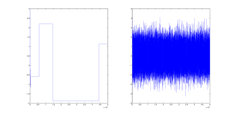
Figure S1: Toy example: The iterates of $\theta$ generated by the independent PM scheme (left) and the block PM scheme (right). Both chains are initialised at 3 and run for 500,000 iterations.

Figure S1 plots the $\theta$-samples generated by the independent PM scheme and by the block PM scheme. As expected, the independent PM chain is sticky because of the big variance $\sigma^{2}=234$ of $z$.

We now study the effect of $\sigma^{2}$ on the acceptance rate and computing time $\text{\rm CT}(\sigma)$ of the block sampler. Figure S2 shows $\text{\rm CT}(\sigma)$ and the acceptance rates for various values of $\sigma^{2}$. The figure shows that $\text{\rm CT}(\sigma)$ has a minimum value of 0.0263 at $\sigma^{2}=234$, where the acceptance rate is 0.279, which agrees with the theory. Pitt et al., (2012) show that the optimal value of $\sigma$ for the independent PM is around 1. We also run this optimal independent PM scheme and obtain a value of the computing time $\text{\rm CT}(\sigma=1)=5.32$. Hence, the optimal block PM is $5.32/0.0263\approx 202$ times more efficient than the optimal independent PM.

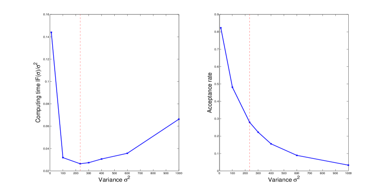
Figure S2: Toy example: The left panel shows the computing time $\text{\rm CT}(\sigma)$ and the right panel shows the acceptance rate v.s. the variance $\sigma^{2}$. The dashed lines indicate the values w.r.t. the optimal variance $\sigma_{\text{\rm opt}}^{2}=234$.

Appendix E Further Applications

E.1 ABC example

$\alpha$-stable distributions (Nolan,, 2007) are heavy-tailed distributions used in many statistical applications. The main difficulty when working with $\alpha$-stable distributions is that they do not have closed form densities, which makes it difficult to do inference. However, one can use ABC to carry out Bayesian inference (Tavare et al.,, 1997; Peters et al.,, 2012), because it is easy to sample from an $\alpha$-stable distribution. Given the observed data $y$, ABC approximates the likelihood by its likelihood-free version

$$L_{\text{LF},\epsilon}(\theta)=\int K_{\epsilon}(S(y^{\prime}),S(y))p(y^{\prime}|\theta){\rm d}\,y^{\prime},$$ (S9)

where $K_{\epsilon}(\cdot,\cdot)$ is a kernel with the bandwidth $\epsilon$ and $S(\cdot)$ is a vector of summary statistics. Inference is then based on the approximate posterior $p_{\text{ABC}}(\theta|y)\propto p_{\Theta}(\theta)L_{\text{LF},\epsilon}(\theta)$, where $L_{\text{LF},\epsilon}(\theta)$ is unbiasedly estimated by $\sum_{i=1}^{M}K_{\epsilon}(S(y^{[i]}),S(y))$, with $y^{[i]}\stackrel{{\scriptstyle iid}}{{\sim}}p(\cdot|\theta)$. Although the likelihood cannot be factorised as in (6), our example illustrates that the block PM scheme still applies.

We use the example in Peters et al., (2012) and generate a data set $y=\{y_{1},...,y_{n}\}$ with $n=200$ observations from a univariate $\alpha$-stable distribution with parameters $\alpha=1.7$, $\beta=0.9$, $\gamma=10$ and $\delta=10$. The characteristic function $\phi_{X}(t)$ of a random variable $X$ following an $\alpha$-stable distribution with parameters $\alpha,\beta,\gamma$ and $\delta$ is

$$\phi_{X}(t)=\begin{cases}\exp\big{(}i\delta t-\gamma^{\alpha}|t|^{\alpha}\big{[}1+i\beta\tan\frac{\pi\alpha}{2}\text{\rm sgn}(t)(|\gamma t|^{1-\alpha}-1)\big{]}\big{)}&\text{if }\alpha\neq 1\\ \exp\big{(}i\delta t-\gamma|t|\big{[}1+i\beta\frac{2}{\pi}\text{\rm sgn}(t)(\log(\gamma|t|)\big{]}\big{)}&\text{if }\alpha=1.\\ \end{cases}$$ (S10)

We use the same summary statistics $S(y^{\prime})=(\widehat{v}_{\alpha}(y^{\prime}),\widehat{v}_{\beta}(y^{\prime}),\widehat{v}_{\gamma}(y^{\prime}),\widehat{v}_{\delta}(y^{\prime}))$ of a pseudo-dataset $y^{\prime}=\{y_{1}^{\prime},...,y_{n}^{\prime}\}$ as in Peters et al., (2012) and refer the reader to that paper for details. We estimate $L_{\text{LF},\epsilon}(\theta)$ in (S9) by $\widehat{L}_{\text{LF},\epsilon}(\theta)=K_{\epsilon}(S(y^{\prime}),S(y))$, with $K_{\epsilon}$ the Gaussian kernel with covariance matrix $\epsilon I_{4}$, using only one pseudo-dataset ($M=1$) as Bornn et al., (2016) show that $M=1$ is optimal.

Both the independent PM and the block PM were run for 50,000 iterations with the first 10,000 discarded as burn-in. The block PM scheme was carried out as follows. Given a vector of parameters $\theta$, write the pseudo-data point $y_{i}^{\prime}$ as $f(\theta,u_{i})$, with $u_{i}$ the set of MC random numbers used to generate $y_{i}^{\prime}$. We divide the set $u=\{u_{i},i=1,...,200\}$ into $G=100$ blocks with the $k$th block $u_{(k)}$ consisting of $u_{2k-1}$ and $u_{2k}$, $k=1,...,G$.

Table S1 summarises the performance measures for different values of $\epsilon$, averaged over 10 runs. In the table, the mean squared error (MSE) is the $l_{2}$-norm of the difference between the estimated posterior mean and the true parameters. See Pasarica and Gelman, (2010) for a definition of average squared jumping distance (ASD) as a performance measure in MCMC. It is understood that the bigger the ASD the better. The results show that the block PM performs better than the independent PM in this example.

$\epsilon$	Methods	Acc. rate	MSE	IACT ratio	ASD
10	IPM	0.31	1.41	2.07	3.14
	BPM	0.37	1.29	1	3.43
2	IPM	0.20	1.14	1.54	0.70
	BPM	0.30	1.17	1	0.96
1	IPM	0.10	0.96	1.75	0.18
	BPM	0.21	0.95	1	0.32

Table S1: ABC example

E.2 State space example

We consider a time series $\{y_{t},t=1,...,T\}$ generated from the non-Gaussian state space model

$$y_{t}|x_{t} \sim \text{Poisson}(\lambda_{t}),\;\;\lambda_{t}=e^{\beta+x_{t}},$$ (S11)

$$x_{t+1} = \phi x_{t}+\eta_{t},\;\;\eta_{t}\sim N(0,\sigma^{2}),\;\;x_{1}\sim N(0,\sigma^{2}/(1-\phi^{2})),$$

with model parameters $\theta=(\beta,\phi,\sigma^{2})$. We generate the data using the parameter values $\beta=1$, $\phi=0.5$ and $\sigma^{2}=2(1-\phi^{2})$, with $T=1000$.

Following Shephard and Pitt, (1997) and Durbin and Koopman, (1997) we write the likelihood $(\theta)$ as

$$L(\theta) =\int p(x_{1}|\theta)p(y_{1}|x_{1},\theta)\prod_{t=2}^{T}p(x_{t}|x_{t-1},\theta)p(y_{t}|x_{t},\theta)\prod_{t=1}^{T}{\rm d}\,x_{t}$$

We employ the high-dimensional importance sampling method of Shephard and Pitt, (1997) and Durbin and Koopman, (1997) to obtain an unbiased likelihood estimator $\widehat{L}(\theta,u)$. The simulation smoothing step requires $2T$ independent univariate normal variates to generate each sample path of the states, so the set of random variates $\bm{u}$ needed is a matrix of size $N\times(2T)$, with $N$ the number of samples. We divide $\bm{u}$ into $G=100$ blocks, where ${{\bm{u}}}_{(1)}$ consists of the first $2T/G$ columns of $\bm{u}$, ${{\bm{u}}}_{(2)}$ consists of the next $2T/G$ columns of $\bm{u}$, etc.

We use the static strategy in this example, i.e. the number of sample paths $N$ is fixed. Let $\bar{\theta}$ be some central value of $\theta$, e.g. the MLE estimate using the simulated maximum likelihood method (Gourieroux and Monfort,, 1995). For simplicity, we set $\bar{\theta}$ to the true value. For the independent PM, we chose the value of $N$ so that ${\mathbb{V}}(\widehat{L}(\bar{\theta},\bm{u}))\approx 1$, where the variance ${\mathbb{V}}(\widehat{L}(\bar{\theta},\bm{u}))$ is estimated by replication. For the two block PM schemes, one using MC and the using RQMC, we select $N$ such that ${\mathbb{V}}(\widehat{L}(\bar{\theta},\bm{u}))\approx 2.16^{2}/(1-\rho^{2})$ and $\approx 0.82^{2}/(1-\rho^{2})$ respectively, with the correlation $\rho$ estimated as follows. Let $z=\log\;\widehat{L}(\bar{\theta},\bm{u})$ and $z^{\prime}=\log\;\widehat{L}(\bar{\theta},\bm{u}^{\prime})$ with $\bm{u}^{\prime}$ obtained from $\bm{u}$ by generating a new set for a randomly-selected block ${{\bm{u}}}_{((k))}$, with the other blocks kept fixed. We generate $J=1000$ realisations $(z_{j},z_{j}^{\prime})_{j=1}^{J}$ of $(z,z^{\prime})$, where a large value $N_{0}$ of $N$ is used, and estimate $\rho$ by the sample correlation $\widehat{\rho}$. For the correlated PM of Deligiannidis et al., (2016), we set the correlation $\varrho=0.99$ and use the same $N$ as in the block PM-MC. Each MCMC scheme was run for 25,000 iterations including a burn-in of 5000 iterations.

Methods	$N$	Acceptance rate	IACT ratio	CPU ratio	TNV ratio
IPM-MC	3500	-	-	-	-
CPM ($\varrho=.99$)	56	0.18	1.613	1.336	2.155
BPM-MC	56	0.23	1.154	1.257	1.451
BPM-RQMC	16	0.23	1	1	1

Table S2: State space example: performance measure ratios with the BPM-RQMC as the baseline

Table S2 summarises the results. We did not run the IPM-MC as it requires $N=3500$ samples, which makes it too computationally demanding. The block PM using RQMC performs the best. Although both the correlated PM and block PM-MC use the same number of samples $N$, the second requires less CPU time because it generates only one block of $\bm{u}$ in each iteration.

References

- Andrieu et al., (2010) Andrieu, C., Doucet, A., and Holenstein, R. (2010). Particle Markov chain Monte Carlo methods. Journal of the Royal Statistical Society, Series B, 72:1–33.
- Andrieu and Roberts, (2009) Andrieu, C. and Roberts, G. (2009). The pseudo-marginal approach for efficient Monte Carlo computations. The Annals of Statistics, 37:697–725.
- Bartolucci et al., (2012) Bartolucci, F., Farcomeni, A., and Pennoni, F. (2012). Latent Markov Models for Longitudinal Data. Chapman and Hall/CRC press.
- Beaumont, (2003) Beaumont, M. A. (2003). Estimation of population growth or decline in genetically monitored populations. Genetics, 164:1139–1160.
- Bornn et al., (2016) Bornn, L., Pillai, N. S., Smith, A., and Woodard, D. (2016). The use of a single pseudo-sample in approximate Bayesian computation. Statistics and Computing, pages 1–8.
- Dahlin et al., (2015) Dahlin, J., Lindsten, F., Kronander, J., and Schön, T. B. (2015). Accelerating pseudo-marginal Metropolis-Hastings by correlating auxiliary variables. Technical report. https://arxiv.org/abs/1511.05483.
- Del Moral, (2004) Del Moral, P. (2004). Feynman-Kac Formulae: Genealogical and Interacting Particle Systems with Applications. Springer, New York.