Self-organisation in protoplanetary disks

Abstract

Context. Recent observations revealed organised structures in protoplanetary disks, such as axisymmetric rings or horseshoe concentrations evocative of large-scale vortices. These structures are often interpreted as the result of planet-disc interactions. However, these disks are also known to be unstable to the magneto-rotational instability (MRI) which is believed to be one of the dominant angular momentum transport mechanism in these objects. It is therefore natural to ask if the MRI itself could produce these structures without invoking planets.

Aims. The nonlinear evolution of the MRI is strongly affected by the low ionisation fraction in protoplanetary disks The Hall effect in particular, which is dominant in dense and weakly ionised parts of these objects, has been shown to spontaneously drive self-organising flows in shearing box simulations. Here, we investigate the behaviour of global MRI-unstable disc models dominated by the Hall effect and characterise their dynamics.

Methods. We validate our implementation of the Hall effect into the PLUTO code with predictions from a spectral method in cylindrical geometry. We then perform 3D unstratified Hall-MHD simulations of keplerian disks for a broad range of Hall, ohmic and ambipolar Elsasser numbers.

Results. We confirm the transition from a turbulent to an organised state as the intensity of the Hall effect is increased. We observe the formation of zonal flows, their number depending on the available magnetic flux and on the intensity of the Hall effect. For intermediate Hall intensity, the flow self-organises into long-lived magnetised vortices. Neither the addition of a toroidal field nor ohmic or ambipolar diffusion drastically change this picture in the range of parameters we have explored.

Conclusions. Self-organisation by the Hall effect is a robust phenomenon in global non-stratified simulations. It is able to quench turbulent transport and spontaneously produce axisymmetric rings or sustained vortices. The ability of these structures to trap dust particles in this configuration is demonstrated. We conclude that Hall-MRI driven organisation is a plausible scenario which could explain some of the structures found in recent observations.

1 Introduction

Protoplanetary discs are the birth place of planets. There are now many observations available, from millimetre wavelengths (ALMA Partnership et al., 2015) to the infrared (Benisty et al., 2015). Surprisingly, these observations indicate that protoplanetary discs have complex internal structures, with features like spiral arms (Muto et al., 2012; Benisty et al., 2015), asymmetric traps (van der Marel et al., 2013) and rings (ALMA Partnership et al., 2015).

The origin of these structures is largely unknown. Most of the theoretical models developed to date involve at least one planet carving a gap (van der Marel et al., 2013; Dipierro et al., 2015) or exciting spiral density waves (Benisty et al., 2015). For this reason, structures are usually seen as a consequence of planet formation. However, the presence of Jupiter mass planets in very young discs such as HL tau is questionable since it implies a very fast formation scenario. It is therefore natural to ask if these structures could appear without planets, and even be one of the driving mechanism behind planet formation. To answer this question, one has to focus on the dynamics of a planet-free disc, a long-standing problem in theoretical astrophysics.

Accretion discs are believed to be subject to the magnetorotational instability (MRI), a magnetohydrodynamic (MHD) instability appearing spontaneously in magnetised discs in Keplerian rotation (Balbus & Hawley, 1991). The relevance of this instability in the context of protoplanetary disc is however debated (Turner et al., 2014). In particular, these objects are so cold that they cannot maintain a large ionisation fraction (Gammie, 1996). This has led to the concept of magnetically “dead” zones where the ionisation fraction of the disc is so low that the standard MHD approach breaks down and the MRI potentially vanishes.

A large effort has recently been devoted to the study of these weakly ionised regions, typically located at radii larger than 1 astronomical unit (a.u.) which are precisely the regions we are now capable of resolving observationally. It has been shown that in this regime, three “non-ideal” effects have to be taken into account in the MHD framework (Balbus & Terquem, 2001; Kunz & Balbus, 2004): Ohmic diffusion, Ambipolar diffusion and the Hall drift. It is well known that both Ohmic and Ambipolar diffusion acts to damp and potentially eliminate the MRI by decoupling the flow from magnetic field lines (Blaes & Balbus, 1994; Jin, 1996; Papaloizou & Terquem, 1997), hence the historical denomination of dead zones. On the other hand, the Hall effect leads to new branches of instabilities (Wardle, 1999; Balbus & Terquem, 2001; Kunz, 2008) due to its dispersive nature.

The saturation of the MRI and the outcome of a disc subject to these non ideal effects is still the subject of intense debate. Stratified models including Ohmic and ambipolar diffusion only have shown that the disc could become essentially laminar (i.e. not turbulent) in the midplane, with a strong magnetically-driven jet at the disc surface (Bai & Stone, 2013; Simon et al., 2013; Gressel et al., 2015). Adding Hall effect leads to a significantly different picture for radii between 1 and 10 a.u. (where Hall effect dominates over diffuse processes) a large-scale midplane stress is found, with a strong field polarity dependence and no turbulence (Lesur et al., 2014; Bai, 2014) whereas the outer disc is found to be essentially insensitive to the Hall effect (Bai, 2015) though some polarity dependence could persist (Simon et al., 2015).

The results of Lesur et al. (2014) and Bai (2014), and in particular the presence of a large-scale “laminar” stress is both an important and potentially problematic result. In effect, these simulations were done in the stratified shearing box framework (Hawley et al., 1995), with a very limited radial extension (typically a few scale height). So Lesur et al. (2014) and Bai (2014) results indicate that the MRI is indeed active in these simulations, but it tends to produce structures larger than the simulation box. As a matter of fact, unstratified shearing box models have already indicated that Hall-dominated MRI is prone to produce large-scale structures such as zonal fields and flows (Kunz & Lesur, 2013, hereafter KL13) in wide enough boxes. All of these elements tend to point toward the fact that the Hall effect could be an efficient mechanism to trigger self-organisation in protoplanetary discs.

In this paper, we explore this hypothesis using full 3D cylindrical models of accretion discs dominated by the Hall-effect. Our aim is not to reproduce the exact structure of a disc with its detailed ionisation equilibrium but to test the hypothesis of self-organisation in a global model, free of the artefacts found in shearing-box simulations. We start by describing in details the physical framework and some remarkable facts concerning Hall dynamics. We then depict our numerical model and present the tests performed to validate it along with a reproduction and discussion of the multifluid models of O’Keeffe & Downes (2014). Next, we move to the core of the paper with the presentation and characterisation of several Hall-dominated models, putting emphasis on the physical mechanisms driving self-organisation. We then explore some potential treats to these mechanisms such as diffusive effects and more complex field configurations. We conclude by discussing the link between these results and recent observations along with extensions of this work to more realistic numerical setups.

2 Framework

2.1 Physical model

We want to model a thin disk of partially ionised gas orbiting a central mass and threaded by a weak magnetic field. At the scales considered, our problem fits in the non-ideal magnetohydrodynamic (MHD) framework. In this attempt to study the Hall effect in global disk simulations, we wish to concentrate on the midplane dynamics, thereby neglecting vertical stratification effects. Using cylindrical coordinates $(r,\varphi,z)$, we take the gravitational force to be oriented radially and assume periodicity in the vertical direction on a scale $h$. Radial stratification is eliminated by using an isothermal disk model with a flat density distribution, and by taking the initial magnetic field to be constant and uniformly vertical over the whole domain.

The relevant equations for our model are those of inviscid, compressible non-ideal MHD. We denote by $\rho$ the bulk density, $\bm{v}$ the bulk velocity, $P=c_{s}^{2}\rho$ the pressure with an isothermal sound speed $c_{s}$, and $\bm{J}=\nabla\times\bm{B}$ the electric current deduced from the magnetic field $\bm{B}=\mid B\mid\bm{e_{b}}$. Gravity is oriented along the cylindrical radius as $\bm{g}=-(1/r^{2})\bm{e_{r}}$. The three relevant non-ideal MHD effects, namely Ohmic dissipation, the Hall effect and ambipolar diffusion, are characterized by their diffusivities $\eta_{\mathrm{O}}$, $\eta_{\mathrm{H}}$ and $\eta_{\mathrm{A}}$ respectively (e.g. Wardle, 2007). With these definitions, the dynamical equations read:

$$\partial_{t}\rho=-\bm{\nabla\cdot}\left[\rho\bm{v}\right],$$ (1)

$$\partial_{t}\left[\rho\bm{v}\right]=-\bm{\nabla\cdot}\left[\rho\bm{v\otimes v}\right]-\bm{\nabla}P+\bm{J\times B}+\rho\bm{g},$$ (2)

$$\partial_{t}\bm{B}=\bm{\nabla\times}\left[\bm{v\times B}-\eta_{\mathrm{O}}\bm{J}-\eta_{\mathrm{H}}\bm{J\times e_{b}}+\eta_{\mathrm{A}}\bm{J\times e_{b}\times e_{b}}\right].$$ (3)

In order to characterize the intensity of the Hall induction term, we use the Alfvén velocity $\bm{v_{A}}=\bm{B}/\sqrt{\rho}$ and introduce the dimensionless parameter

$$\mathcal{L}\equiv\ell_{\mathrm{H}}/h$$ (4)

ratio of the Hall length $\ell_{\mathrm{H}}\equiv\eta_{H}/v_{A}$ as defined in Kunz & Lesur (2013) (hereafter KL13) and the geometric scale height of the disk. The Hall length is very convenient as it only depends on the microphysical properties of the plasma and not on the field strength. In a plasma made of electrons, singly charged ions and neutrals, the Hall length is given by

$$\ell_{H} =\Bigg{(}\frac{c^{2}m_{i}}{4\pi e^{2}n_{e}}\Bigg{)}^{1/2}\Bigg{(}\frac{\rho}{\rho_{i}}\Bigg{)}^{1/2}$$ (5)

$$=0.14\,\Bigg{(}\frac{\rho}{10^{-9}\,\mathrm{g.cm}^{-3}}\Bigg{)}^{-1/2}\Bigg{(}\frac{\xi}{10^{-12}}\Bigg{)}^{-1}\,\mathrm{a.u},$$ (6)

where $m_{i}$ is the ion mass, $n_{e}$ is the electron number density and $\rho_{i}$ is the ion density. The numerical value has been obtained assuming a plasma made of electrons, heavy ions and neutral molecules (mean molecular mass $\mu=2.34\,m_{\mathrm{H}}$) with an ionisation fraction $\xi$. The precise calculation of the Hall length involves solving a complex chemical network and depends on the presence and size distribution of grains, which is beyond the scope of this paper. We note however that typical values for $\mathcal{L}$ range from $\mathcal{L}\sim 100$ at 5 a.u. down to $\mathcal{L}\sim 10^{-2}$ at 100 a.u. for $1\,\mu\mathrm{m}$ size grains (e.g. Simon et al., 2015), smaller grains leading to larger values of $\mathcal{L}$. The Hall effect being a dispersive term, it induces a strong Courant-Friedrichs-Lewy (CFL) constraint on the timestep of our explicit scheme. For this reason, we restrict ourselves to simulations with $\mathcal{L}\leq 10$ to keep computation times within reasonable bounds.

Most of our simulations neglect ohmic and amibipolar diffusion to focus on Hall-MHD only. We however briefly explore the impact of these diffusion terms on our results in section 6. It is customary to quantify the importance of diffusion terms via the Lundquist and Elsasser numbers respectively defined by

$$\mathcal{S}_{\mathrm{O},\mathrm{A}}\equiv\frac{v_{A}h}{\eta_{\mathrm{O},\mathrm{A}}},\qquad\Lambda_{\mathrm{O},\mathrm{A}}\equiv\frac{v_{A}^{2}}{\eta_{\mathrm{O},\mathrm{A}}\Omega},$$ (7)

where the index stands for ohmic or ambipolar diffusion. When setting the value of these parameters, it will be with respect to the initial Alfvén velocity $B_{0}/\sqrt{\rho_{0}}$.

In this paper, we wish to exclude most stratification effects. Since we do not solve for the chemistry of the disk, fixing a constant $\ell_{\mathrm{H}}$ gives a natural extension of the local simulations of KL13. We choose to set $\eta_{O}$ constant so that $\mathcal{S}_{\mathrm{O}}$ describes a disk that is either globally stable or unstable to the MRI (Jin, 1996). Most previous studies on ambipolar diffusion were conducted at a given $\Lambda_{\mathrm{A}}$, but with a constant Alfvén velocity this corresponds to a disk gradually stabilised by the diffusivity $\eta_{\mathrm{A}}\propto r^{3/2}$. We choose instead to use a constant ion-neutral coupling time $\tau_{\mathrm{A}}$ so that $\eta_{\mathrm{A}}(\bm{r},t)=\tau_{\mathrm{A}}v_{A}(\bm{r},t)^{2}$ everywhere and at all time. With an initially constant Alfvén velocity, the initial $\mathcal{S}_{\mathrm{A},0}=h/\tau_{\mathrm{A}}v_{A,0}$ is constant too, making the disk globally unstable and facilitating comparison with the ohmic case.

2.2 Simplified model of Hall dynamics

We point out some properties derived from the dynamical equation (3), and refer the reader to the section 4 of KL13 for a discussion about the following model.

Discarding the ambipolar and ohmic terms, and assuming a constant Hall length, the induction equation of Hall MHD reads

$$\partial_{t}\bm{B} =\bm{\nabla\times}\left[\bm{v\times B}-\ell_{\mathrm{H}}\bm{J\times B}\right]$$

$$=\bm{\nabla\times}\left[\bm{v\times B}\right]-\ell_{\mathrm{H}}\bm{\nabla\times}\left[\bm{\nabla\cdot}\left(\bm{B\otimes B}\right)\right].$$ (8)

For illustrative purposes we use the shearing box model to remove curvature terms; we can then average over the periodic vertical and azimuthal directions and obtain the simplified equation

$$\begin{split}\partial_{t}\left\langle\bm{B}_{z}\right\rangle_{yz}&=\left\langle\bm{\nabla\times}\left[\bm{v\times B}\right]_{z}\right\rangle-\ell_{\mathrm{H}}\left\langle\bm{\nabla\times}\left[\bm{\nabla\cdot}\left(\bm{B\otimes B}\right)\right]_{z}\right\rangle\\ &\simeq\eta_{t}\frac{\partial^{2}}{\partial x^{2}}\left\langle B_{z}\right\rangle-\ell_{\mathrm{H}}\frac{\partial}{\partial x^{2}}\left\langle B_{x}B_{y}\right\rangle\end{split}$$ (9)

where we have approximated the ideal MHD term by a turbulent resistivity (Lesur & Longaretti, 2009). This expression shows that in the presence of the Hall effect, the horizontal Maxwell stress appears explicitly in the induction equation. Since this component of the stress also drives the transport of angular momentum (Balbus & Papaloizou, 1999), this expression implies a tight connection between the transport of angular momentum and that of vertical magnetic flux tubes. These relations will prove useful in understanding our results.

2.3 Linear stability

We recall that in Hall MHD, differentially rotating flows embedded in a magnetic field can be subject to the Hall-shear instability (HSI), different in essence from the magneto-rotational instability (Kunz, 2008). Indeed, angular-momentum conservation is central to the MRI mechanism, whereas the HSI relies only on electric currents and needs not disturb the bulk of the flow. One other fundamental difference is the dependence of the HSI on the orientation of the magnetic field with respect to the rotation axis. In the case favorable to instability ($\bm{\Omega\cdot B}>0$), it can be shown (Simon et al., 2015) that the HSI develops when the local shear frequency is larger than the whistler frequency at the considered wavenumber $k$, that is :

$$q\Omega\geq\ell_{\mathrm{H}}v_{A}k^{2}$$ (10)

with $q\equiv|\,\mathrm{d}\log\Omega/\mathrm{d}\log r\,|=3/2$ in our non-stratified keplerian case. Given a constant $\ell_{\mathrm{H}}$, we see that the flow will be Hall-shear stable for all wave numbers down to the minimal $k_{0}=2\pi/h$ for Alfvén velocities above the critical value

$$v_{A,\mathrm{crit}}\equiv\frac{3\Omega_{0}h^{2}}{8\pi^{2}\ell_{\mathrm{H}}}\Bigg{(}\frac{r}{r_{0}}\Bigg{)}^{-3/2}.$$ (11)

2.4 Diagnostics

We use brackets to denote space averaging, with subscript indicating the coordinate over which a function is integrated:

$$\left\langle f\right\rangle_{z} \equiv\frac{1}{h}\int_{z=-h/2}^{h/2}f\,\mathrm{d}z,$$ (12)

$$\left\langle f\right\rangle_{r\varphi} \equiv\frac{2}{(r_{out}^{2}-r_{in}^{2})\Delta\varphi}\int_{r=r_{in}}^{r_{out}}\int_{\varphi=0}^{\Delta\varphi}f\,r\,\mathrm{d}\varphi\,\mathrm{d}r,$$ (13)

with $r_{in}$ and $r_{out}$ delimiting the active computational domain and $\Delta\varphi$ the angular extent of the disk. Subscripts will be omitted when obvious from the context. We use an overline for the time averaging of an already volume-averaged quantity :

$$\overline{f}\equiv\frac{1}{T}\int_{t=t_{0}}^{t_{0}+T}\left\langle f\right\rangle\,dt.$$ (14)

As a characterization of the spatial coherence of the flow, we use the auto-correlation function

$$\mathcal{A}_{y,z}[f](x)\equiv\frac{\int f(t,y,z)f(t+x,y,z)\,\mathrm{d}t}{\int f(t,y,z)^{2}\,\mathrm{d}t}$$ (15)

and define a normalized correlation factor

$$\mathcal{C}_{z}[f](r,\varphi)\equiv\frac{1}{h}\int_{z=-h/2}^{h/2}\mathcal{A}_{r,\varphi}[f](z)\,\mathrm{d}z$$ (16)

equal to unity where the correlation length is equal to the height $h$. We also use $\mathcal{C}_{\varphi}[f](r,z)$ defined by substituting $\varphi$ and $z$ and replacing $h$ by the angular extent $\Delta\varphi$.

Following Balbus & Papaloizou (1999), the turbulent Reynolds stress tensor is defined with the velocity fluctuations about the density weighted averaged flow: $\mathcal{R}\equiv\rho\tilde{\bm{v}}\otimes\tilde{\bm{v}}$ where $\tilde{\bm{v}}=\bm{v}-\left\langle\rho\bm{v}\right\rangle_{\varphi z}/\left\langle\rho\right\rangle_{\varphi z}$. The Maxwell stress tensor is simply defined as $\mathcal{M}\equiv-\bm{B}\otimes\bm{B}$. We introduce two dimensionless measures of turbulent stress; the first one is the usual $\alpha$ parameter of Shakura & Sunyaev (1973):

$$\alpha_{\mathrm{SS}}\equiv\frac{\mathcal{R}_{r\varphi}+\mathcal{M}_{r\varphi}}{\rho c_{s}^{2}}.$$ (17)

Since we work in a cylindrical setup, an alternative definition for $\alpha$ is possible using $\Omega$ and the characteristic length $h$. We thus define

$$\alpha_{\mathcal{R}}\equiv\frac{\mathcal{R}_{r\varphi}}{\rho\Omega^{2}h^{2}},\qquad\alpha_{\mathcal{M}}\equiv\frac{\mathcal{M}_{r\varphi}}{\rho\Omega^{2}h^{2}},\qquad\alpha\equiv\alpha_{\mathcal{R}}+\alpha_{\mathcal{M}}.$$ (18)

It should be emphasized again that in a disk in true hydrostatic equilibrium, $c_{s}^{2}=\Omega^{2}h^{2}$ so that $\alpha_{\mathrm{SS}}=\alpha$. In a cylindrical system such as ours, this equality does not hold anymore and one has to pick (17) or (18). In the following, we use (18) as our main diagnostic since the fluctuations are essentially incompressible, making the sound speed less relevant physically than the geometrical velocity $\Omega h$.

2.5 Units

We take the inner radius $r_{0}$ and the keplerian velocity at the inner radius $v_{0}$ as distance and velocity units, resulting in a natural frequency unit $\Omega_{0}\equiv v_{0}/r_{0}$. Time is expressed relative to the orbital period at the inner radius $T_{0}\equiv 2\pi/\Omega_{0}$, and density relative to the initial constant density $\rho_{0}$. Magnetic field strength is expressed as an Alfvén velocity $B/\sqrt{\rho_{0}}$, and the initial vertical magnetic field is always denoted $B_{0}$. We will also use the initial thermal pressure $P_{0}\equiv\rho_{0}c_{s}^{2}$.

3 Method and validation

3.1 Description

3.1.1 Numerical scheme

The dynamical equations (1)-(3) are explicitly integrated in time with a modified version of the finite volume code PLUTO (Mignone et al., 2007) in 3D cylindrical geometry. The magnetic field is evolved with the constrained transport method (Evans & Hawley, 1988), preserving $\nabla\cdot\bm{B}=0$ to machine precision.

Our implementation of the Hall effect is the same as that described in Appendix A of Lesur et al. (2014): the Hall induction flux is incorporated in a conservative manner within a modified HLL Riemann solver. Since the Hall effect introduces dispersive waves, the whistler speed required when computing Godunov fluxes is truncated at the grid scale in the direction under consideration. The face-centered electric currents must be provided to this solver as an external parameter. These are computed by finite difference of either the volume-averaged or the face-centered magnetic field of neighbouring cells, according to the cylindrical expression for the curl operator.

We use a second-order accurate Runge-Kutta time-integration scheme, a piecewise linear space reconstruction of the fields within each cell, and the Van Leer slope limiter. The FARGO module (Mignone et al., 2012) is employed to substantially increase the initial timesteps and reduce the numerical diffusivity due to the advection by the mean Keplerian flow.

3.1.2 Grid and boundary conditions

Our computational domain is cylindrical, truncated in the azimuthal direction to quarter disks $\Delta\varphi=\pi/2$ for all runs except one $2\pi$ full disk, saving computational time while revealing global effects already. The ratio of the cylinder height $h$ to its inner radius $r_{0}$ is fixed to $1/4$ for all simulations, consistently with our thin disk assumption. We set the outer radius at $5r_{0}$, giving an aspect ratio of $16$. The sound speed is fixed to $10\%$ of the keplerian velocity at the inner radius, so that our geometrical scale height $h$ is of the order of the hydrostatic pressure scale height $c_{s}/\Omega$ in the computational domain, being equal at $r\simeq 1.8r_{0}$. This domain is meshed with 32 grid cells in the vertical direction, 512 uniformly distributed cells in the radial and azimuthal directions (2048 azimuthal cells for the $2\pi$ run), giving a square mesh in the $\left(r,z\right)$ plane and an almost cubic grid at $r\approx 2.5r_{0}$.

All runs are initialised with a density $\rho=\rho_{0}$ on the whole domain, a keplerian azimuthal velocity field $v_{\varphi}=r^{-1/2}$ and uniform $B_{z}=B_{0}$. The vertical and azimuthal boundary conditions are periodic. Special care was taken with the radial boundary conditions, for they can drastically affect the physics in the computational domain. The same type of conditions are imposed at the two radial boundaries; unless otherwise stated they are as follows: the radial and vertical velocities vanish as well as the radial derivative of the density; the azimuthal velocity is set to its initial keplerian value; the azimuthal component of the magnetic field is forced to zero while the vertical component is set to $B_{0}$, and the radial component follows from the divergence free condition.

Boundary conditions alone allow the development of large-scale quasi-steady spiral waves within the domain in purely hydrodynamical setup. These undesirable effects appeared for a variety of boundary conditions, so we chose to add damping buffer zones to smooth the transition from the active domain to the boundaries and smooth these structures out. The buffers span a radial extent $h$ from both radial boundaries, where all hydrodynamical fields are linearly relaxed over time. They are excluded from all subsequent space-averagings.

In the half of the buffer closest to the boundary, all velocity components are brought back to their initial value with an exponential relaxation: $\bm{v}\mapsto\bm{v}-S_{1}(r)(\bm{v}-\bm{v_{0}})\delta t/\tau$, with characteristic time scale $\tau=0.125/\Omega(r)$, and with a linear modulation $S_{1}(r)$ such that the relaxation is fully active at the boundary and vanishes at the middle of the buffer.

In the whole buffer, the density is relaxed in the following manner. First, the average radial density distribution $\left\langle\rho\right\rangle_{\varphi z}(r)$ is computed. Let $r_{b}$ be the radius of the edge of the current buffer. In each cell the density is relaxed exponentially in time to the arithmetic mean between the local average density and the average at the edge of the buffer:

$$\rho(r,\varphi,z)\mapsto\rho(r,\varphi,z)-S_{2}(r)\left[\left\langle\rho\right\rangle(r)-\left\langle\rho\right\rangle(r_{b})\right]\frac{\delta t}{2\tau},$$ (19)

where $S_{2}(r)$ is again a linear modulation equal to one at the boundary and zero at $r_{b}$.

This separation into two sub-buffers helps preventing an accumulation of mass between the buffer and the active domain, avoiding the formation of a local minimum of potential vorticity and keeping the flow Rossby stable (Lovelace et al., 1999). Also, relaxing the density to its average value from the active domain mimics outflow conditions and allows long time behavior such as a density drop by accretion to take place.

We impose a constant resistivity $\eta_{b}=4\times 10^{-4}$ in the buffers, stabilizing the MRI for typical magnetic field intensities without affecting the CFL condition. Moreover, in Hall MHD simulations we linearly decrease the Hall length from the active domain and make it vanish at the boundaries, avoiding unnecessary Hall drift waves at the interface.

Finally, after a first round of simulations we found that magnetic flux losses were sometimes too large to maintain a near statistically steady system. This prevented us from computing proper time averages and comparing our results with previous works. Part of this monotonic decrease in net flux comes from turbulent accretion / excretion of mass out of the computational domain, but it is amplified by the Hall term

$$\partial_{t}\langle B_{z}\rangle_{r\varphi}\simeq\oint\ell_{\mathrm{H}}\mathrm{d}\bm{l\cdot}(\bm{\nabla\cdot\mathcal{M}}),$$ (20)

always negative since we damp the Maxwell stress in the buffers with ohmic diffusion. This term inputs negative flux from the boundaries, which spreads to the active domain and progressively stabilizes the flow. We thus renormalise the total vertical magnetic flux at each time step in the active domain $B_{z}(r,\varphi,z)\mapsto B_{z}(r,\varphi,z)-\left\langle B_{z}\right\rangle+\left\langle B_{0}\right\rangle$. This way, we obtain quasi-steady states in all of our regimes. In the ideal-MHD case, the amount of magnetic flux thus added varies between $10\%$ and $30\%$ of the initial magnetic flux over $200T_{0}$, the larger flux losses corresponding to the higher transport rates, occurring for higher initial net flux. In the strong-Hall regime, less than $5\%$ of the total flux is lost from $50T_{0}$ to $200T_{0}$ in the organized phase. These flux losses are small on a dynamical time scale, and we verified that the maximal turbulent stress attained in time were the same with and without this procedure. The qualitative level of self-organisation was also consistent between runs with and without the flux renormalisation. One caveat of this method is that mass losses should enhance the turbulent stress in time as the relative importance of magnetic to thermal pressure increases (Hawley et al., 1995).

3.2 Validation

We developed a Chebyshev pseudo-spectral method to compute the MRI eigenmodes in axisymmetric cylindrical coordinates, described in appendice A. It includes viscosity and all three non-ideal MHD effects, and was tested in ideal, ohmic, Hall and ohmic plus Hall configurations.

The method returns the axisymmetric eigenmodes of the non-ideal MHD equations, linearized about a stationnary keplerian flow with uniform vertical magnetic field. In this section, we take the computational domain to be the unit square $\left(r,z\right)\in\left[1,2\right]^{2}$. The boundary conditions are periodic in $z$, with vanishing $v_{r}$, $v_{\varphi}$ and $B_{\varphi}$, $\partial_{r}v_{z}$ and $\partial_{r}B_{z}$ at the radial boundaries.

We compare the profiles predicted with a resolution of 256 spectral modes to the result of direct numerical simulations (DNS) on a $256^{2}$ grid. The initial and boundary conditions implemented in PLUTO are the same as those of the spectral method, with a white noise of amplitude $\delta v/c_{s}<10^{-10}$ seeded in the $v_{r}$ and $v_{z}$ fields. The fastest growing MRI mode rapidly dominates, and the growth is slow enough that we can extract the radial profiles at a given height, normalize them so that they have the same amplitude and compare them to linear predictions.

We show in Fig. 1 a comparison of the MRI linear modes including both ohmic diffusion and the Hall effect. This setup has $B_{0}=2\times 10^{-3}$, $\eta_{O}=3\times 10^{-3}$ and $\ell_{\mathrm{H}}=1.0$, and would be linearly stable in the absence of the Hall effect because of Ohmic damping with $\mathcal{S}_{\mathrm{O}}<1$ (Jin, 1996). Five of these normalized radial profiles are drawn in Fig. 1. These profiles show that our DNS implementation accurately reproduces the spectral predictions, with an average error of the order $10^{-3}$.

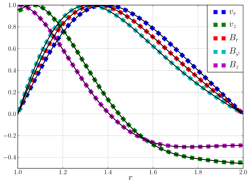
Figure 1: Radial profiles of the fastest growing cylindrical MRI eigenmode for $B_{0}=2\times 10^{-3}$, $\eta_{O}=3\times 10^{-3}$ and $\ell_{\mathrm{H}}=1.0$; comparison between the predictions (solid lines) and DNS (squares).

For this particular setup, the measured growth rate $\gamma=0.0988$ matches the predicted rate $\gamma_{0}=0.0989$ (see Fig. 2). In all our tests, the predicted growth rate fit to better than $10^{-3}$ in relative accuracy with measurements from DNS. The same linear analysis was performed in 3D cylindrical coordinates with only one computational grid cell in the azimuthal direction, so that we preserve the axisymmetric conditions while testing the 3D implementation of the code. Finally, we ensured that the 2D and 3D implementations gave similar results in the non-linear phase for similar initial conditions.

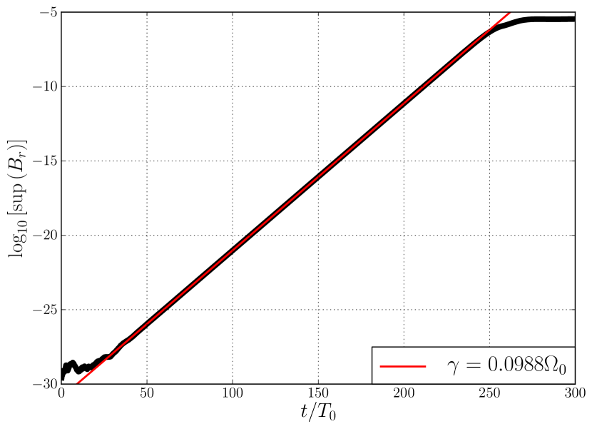
Figure 2: Exponential growth of the perturbed magnetic field $B_{r}$.

3.3 Comparison with previous works

The only global simulations including the Hall effect published to date are those of O’Keeffe & Downes (2014). Their setup being similar to ours, it it is natural to begin our report with a comparative study. We wish to reproduce their highest resolution simulations for the two orientations of the initially axial magnetic field with respect to the rotation axis: Up for aligned (corresponding to run ‘res4-mf’) and Down for oppositely directed (corresponding to their run ‘480-mf-minusbz’).

We first convert their units into ours and get the following values (see appendix B): the computational domain is $\left(r,\varphi,z\right)\in\left[1,5.2\right]\times\left[0,\pi/2\right]\times\left[0,0.39\right]$, meshed with a grid $480\times 480\times 36$. The isothermal sound speed is fixed to $c_{s}=4.35\times 10^{-2}$, the initial magnetic field is $B_{0}=2.2\times 10^{-3}$ and the Hall length is $\ell_{\mathrm{H}}=5.5\times 10^{-3}$. We integrate the dynamical equations on a longer time interval of 130 inner orbits in order to see if the total magnetic energy grows exponentially as seen by O’Keeffe & Downes (2014) on their figure 13. They also report the appearance of transient waves exciting resonant modes from the radial boundaries, motivating the inclusion of damping buffer zones. We used similar buffers of width $0.2r_{0}$ where the hydrodynamical variables $\rho$ and $\bm{v}$ are relaxed to their initial values on a characteristic time of one local orbital period. In addition, we chose to maintain the total vertical magnetic flux and mass constant within the active domain, using the procedure described in 3.1.2 both for $B_{z}$ and $\rho$. This modification of the original setup was necessary in order to keep a quasi-steady turbulent state and measure a statistically meaningful difference between the two runs ; otherwise, mass and flux losses where about twice larger in the first stage of run Up compared to run Down, after which both runs had a compatible level of turbulent stress slowly decreasing with time

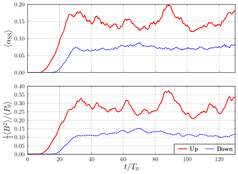
Figure 3: Space-averaged $\alpha_{\mathrm{SS}}$ parameter (upper panel) and total magnetic energy (lower panel) over time, in the active domain for the two comparison runs Up (solid red) and Down (dashed blue).

We show in Fig. 3 the evolution in time of the space-averaged $\left\langle\alpha_{\mathrm{SS}}\right\rangle$ and the total magnetic energy for the two runs, corresponding to the figures 12 and 13 from O’Keeffe & Downes (2014).

We find a slightly lower linear growth rate in run Down, in agreement with the fact that axisymmetric configurations are stabilised by the Hall effect when the magnetic field is anti-aligned with respect to the rotation axis (Balbus & Terquem, 2001). During the steady turbulent phase from $60T_{0}$ to $130T_{0}$, we measure $\overline{\alpha_{\mathrm{SS}}}=\left(1.5\pm 0.2\right)\times 10^{-1}$ in run Up and $\overline{\alpha_{\mathrm{SS}}}=\left(7.4\pm 0.5\right)\times 10^{-2}$ in run Down, larger than the results of O’Keeffe & Downes (2014) by a factor $2$ for run Up and a factor $8$ for run Down. However, we can compare these values with the local Hall-MHD simulations Z2L and Z4L of Sano & Stone (2002), where they used similar input parameters in extended shearing-boxes: $B_{0}=\pm 2.5\times 10^{-3}$, $\ell_{\mathrm{H}}\simeq v_{A}/\Omega\approx 5.5\times 10^{-3}$ at radius $1.8r_{0}$, plus an additional resistivity such that $\Lambda_{\mathrm{O}}=100$, large enough to impact only in a minor way the saturation level of the turbulence. These two runs yielded $\overline{\alpha_{\mathrm{SS}}}\approx 2\times 10^{-1}$ in Z2L (Up case) and $\overline{\alpha_{\mathrm{SS}}}\approx 8\times 10^{-2}$ in Z4L (Down case), similar to our results both in magnitude and ratio.

Concerning the total magnetic energy, we do not observe a long-term growth as reported by O’Keeffe & Downes (2014). The total magnetic energy is about twice larger in run Up compared to run Down, scaling as the ratio of stresses in accordance with previous studies of MRI-induced turbulence in local ideal MHD simulations (see e.g. Minoshima et al., 2015, figure 2). The mean magnetic energy density is $1.2\times 10^{-1}\rho_{0}c_{s}^{2}$ in run Down, comparable again to run Z4 of Sano & Stone (2002) (see their figure 1). It is possible that the long-term exponential growth found by O’Keeffe & Downes (2014) both in turbulent stress and in magnetic energy (their figures 12 to 15) reflects a state that is not converged yet, whence our larger values for $\alpha_{\mathrm{SS}}$.

We do observe the formation of structures such as gaps close to the inner and outer boundaries, but we attribute them to the damping buffer zones for the density accumulates precisely at the edge between the the inner buffer and the active domain. This is the kind of density structures we want to avoid with our own buffers implementation as described in section 3.1.2. Finally, note that the strong turbulent activity ($\alpha_{\mathrm{SS}}\sim 10^{-1}$) is due to the large geometrical thickness of the disk compared to its pressure scale height near the inner boundary ($\Omega h\gg c_{s}$). For this reason, turbulence becomes transonic and strong density waves develop. This unrealistic feature is absent from our other 3D runs for which we enforce $\Omega h\lesssim c_{s}$.

4 Results

4.1 Numerical protocol

All of the global simulations to date have been computed in the weak Hall regime ($\ell_{\mathrm{H}}/h\ll 1$) which only moderately affect the dynamics of the system. However, disks are known to exhibit regions with much stronger Hall effect, in particular in the so called “dead zone” between 1 and 10 a.u. (Lesur et al., 2014). In these regions, we expect $\ell_{\mathrm{H}}/h$ of the order of 10 in the disk midplane. In this section we focus on this regime and on its impact on the global disk dynamics.

The integration time varied from one run to another depending on the steadiness of the flow, with a default lower bound of 200 inner orbits, that is about 18 orbits at the outer radius. The boundary conditions are those described in section 3.1.2. We ensured that the purely hydrodynamic case was stable, with only faint spiral waves coming from the inner boundary ($\delta v_{r}/c_{s}\sim\delta\rho/\rho_{0}\lesssim 10^{-4}$).

As we are mostly interested in the non-linear evolution of the system, we initialise the flow in a specific way. We start from a keplerian flow in ideal MHD, threaded by a constant vertical magnetic field $B_{0}=10^{-3}$. Perturbations are added to the three components of the velocity field with a large amplitude $\delta v/c_{s}=10\%$, so that MRI modes rapidly develop on the entire domain. After $t\approx 30T_{0}$, the MRI saturates and we stop the simulation at $t=50T_{0}$ in a fully turbulent configuration as illustrated in Fig. 4. Only $3\%$ of the total mass has left the box at that moment, equally from the inner and outer radial boundaries. The radial profile of $\left\langle\rho\right\rangle_{\varphi z}$ is decreased by about $10\%$ close to the radial boundaries, and density waves create fluctuations of about $0.1\rho_{0}$ in the active domain. The turbulent state thus obtained is not subject to a radial density stratification.

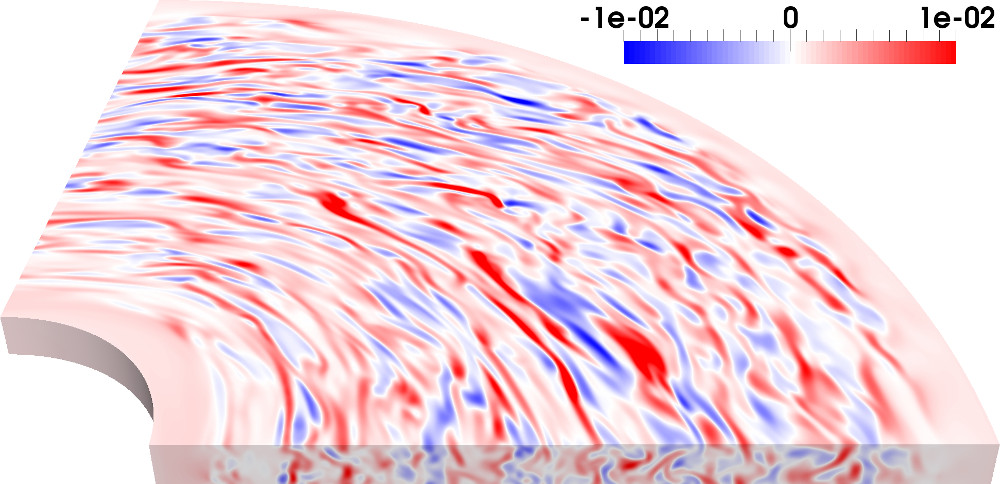
Figure 4: Vertical magnetic field in the turbulent flow when switching on the Hall effect, at $t=50T_{0}$.

All subsequent runs are launched from this configuration, with non-ideal effects switched on and with the net magnetic flux fixed to the desired value. Apart from saving $50T_{0}$ of computational time, this method allows us to have the same initial conditions for all runs, and to have initial conditions that are turbulent over the whole domain so that self-organisation processes cannot be attributed to an excessively symmetric initial state. The parameters used in the following 3D Hall MHD runs are listed in table 1.

We have not systematically explored negative mean field configurations $\bm{B}_{0}\bm{\cdot\Omega}<0$. Effectively, the Hall effect is known to be sensitive to the field polarity. In particular, the vertical field configuration we present is known to be stable for negative weak field strengths (Balbus & Terquem, 2001):

$$|v_{A}|<\frac{\Omega\ell_{H}}{2}\quad\quad\mathrm{STABILITY}.$$ (21)

This implies that sub-equipartition magnetic fields are necessarily stable in the negative polarity configuration when $\mathcal{L}=O(1)$. We have checked successfully that it was the case in our numerical simulations, and we won’t discuss this case any further. Note however that configurations with a strong mean toroidal field can still become unstable, as demonstrated by Simon et al. (2015).

Simulations with net vertical magnetic flux Name $\Delta\varphi$ $T_{s}$ $B_{0}$ $\mathcal{L}$ $\overline{\alpha}$ state B3L0 $\pi/2$ $200$ $10^{-3}$ $0$ $5.6\times 10^{-2}$ turbulent B3L1 $\pi/2$ $200$ $10^{-3}$ $0.02$ $7.8\times 10^{-2}$ turbulent B3L2 $\pi/2$ $200$ $10^{-3}$ $0.04$ $9.8\times 10^{-2}$ turbulent B3L3 $\pi/2$ $200$ $10^{-3}$ $0.1$ $1.4\times 10^{-1}$ turbulent B3L4 $\pi/2$ $200$ $10^{-3}$ $0.2$ $8.2\times 10^{-2}$ turbulent B3L5 $\pi/2$ $200$ $10^{-3}$ $0.4$ $1.6\times 10^{-2}$ 1 band B3L6 $\pi/2$ $300$ $10^{-3}$ $1$ $4.8\times 10^{-4}$ 4 bands 2$\pi$L4 $2\pi$ $200$ $10^{-3}$ $0.2$ $1.7\times 10^{-1}$ turbulence 2$\pi$L5 $2\pi$ $400$ $10^{-3}$ $0.4$ $1.8\times 10^{-2}$ vortex 2$\pi$L6 $2\pi$ $200$ $10^{-3}$ $1$ $1.2\times 10^{-3}$ 3 bands B4L0 $\pi/2$ $200$ $10^{-4}$ $0$ $3.8\times 10^{-3}$ turbulent B4L1 $\pi/2$ $300$ $10^{-4}$ $0.02$ $1.7\times 10^{-2}$ turbulent B4L2 $\pi/2$ $200$ $10^{-4}$ $0.04$ $3.7\times 10^{-2}$ turbulent B4L3 $\pi/2$ $200$ $10^{-4}$ $0.1$ $8.2\times 10^{-2}$ turbulent B4L4 $\pi/2$ $200$ $10^{-4}$ $0.2$ $6.2\times 10^{-2}$ turbulent B4L5 $\pi/2$ $400$ $10^{-4}$ $0.4$ $1.7\times 10^{-2}$ vortex B4L6 $\pi/2$ $300$ $10^{-4}$ $1$ $3.8\times 10^{-4}$ 1 band B4L7 $\pi/2$ $300$ $10^{-4}$ $2$ $5.1\times 10^{-4}$ 3 bands B5L1 $\pi/2$ $200$ $10^{-5}$ $0.1$ $7.6\times 10^{-2}$ turbulent B5L2 $\pi/2$ $200$ $10^{-5}$ $0.2$ $6.4\times 10^{-2}$ turbulent B5L3 $\pi/2$ $300$ $10^{-5}$ $0.4$ $1.1\times 10^{-2}$ vortex B5L4 $\pi/2$ $300$ $10^{-5}$ $1$ $4.4\times 10^{-4}$ 1 band B5L5 $\pi/2$ $200$ $10^{-5}$ $2$ $8.5\times 10^{-4}$ 3 bands B5L6 $\pi/2$ $200$ $10^{-5}$ $4$ $2.5\times 10^{-4}$ 5 bands B5L7 $\pi/2$ $200$ $10^{-5}$ $10$ $3.7\times 10^{-4}$ 3 bands

Table 1: Parameters for the 3D Hall MHD runs: label of the run, integration time $T_{s}$, mean vertical magnetic field $B_{0}$, Hall parameter $\mathcal{L}$, total turbulent stress $\overline{\alpha}$, and final state of the flow.

4.2 Turbulence

Our study starts by sampling $\mathcal{L}$ for different values of the global magnetic flux. We wish to find whether the transition from high to low transport states found in KL13 still occurs in cylindrical geometry, how it depends on the available net flux, and to characterize these states in terms of turbulent stress and critical $\mathcal{L}$.

In Fig. 5 are drawn the profiles of normalized Reynolds and Maxwell stress for the ideal-MHD run B3L0 and the Hall MHD run B3L3. Since we kill the MRI within the buffer zones, the stress has to vanish at the boundaries of the active domain, attaining its maximum near $3.5r_{0}$. We note a local increase of Reynolds stress near the outer boundary, possibly due to a characteristic damping time too long in the outer buffer. The profile of Maxwell stress is essentially shifted of a factor two higher by the Hall effect; the Reynolds stress does not increase as much, but we show on the lower panel that the ratio of Maxwell to Reynolds stress profiles remains roughly constant with radius in both runs with a value $\mathcal{M}/\mathcal{R}\approx 2$ in ideal MHD and $3$ in Hall-MHD, comparable to previous shearing box simulations (see e.g. Hawley et al., 1995).

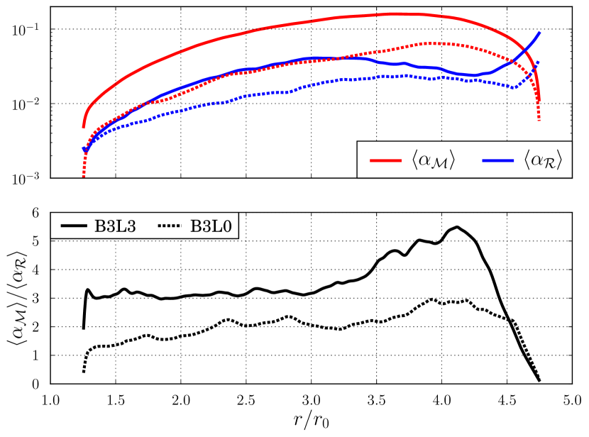
Figure 5: Upper panel: radial profiles of the magnetic (red) and kinetic (blue) contribution to $\alpha$ in runs B3L3 (solid line) and B3L0 (dashed line); lower panel: ratio of Maxwell to Reynolds stress in the same runs. The time averaging is performed between $100T_{0}$ and $200T_{0}$.

For all the runs with $\mathcal{L}\in\left[0,1\right]$, we approximately reach a statistically steady state at the end of the simulation, and average the global turbulent stress in time over at least $50T_{0}$ ($100T_{0}$ in most cases). These values of $\overline{\alpha}$ are presented in Fig. 6 against the corresponding value of $\mathcal{L}$. We find a good qualitative agreement with the figure 11 of KL13: the turbulent activity is enhanced for small $\mathcal{L}$ (orange region in Fig. 6), reaching its peak value for $\mathcal{L}\approx 0.1$ at all $B_{0}$, beyond which the system forks to a low-transport state with a mean stress significantly lower than in the ideal MHD case. We also find that the stress increases with $B_{0}$ for $\mathcal{L}<0.1$ in accordance with previous ideal-MHD local simulations (e.g. Sano & Stone, 2002).

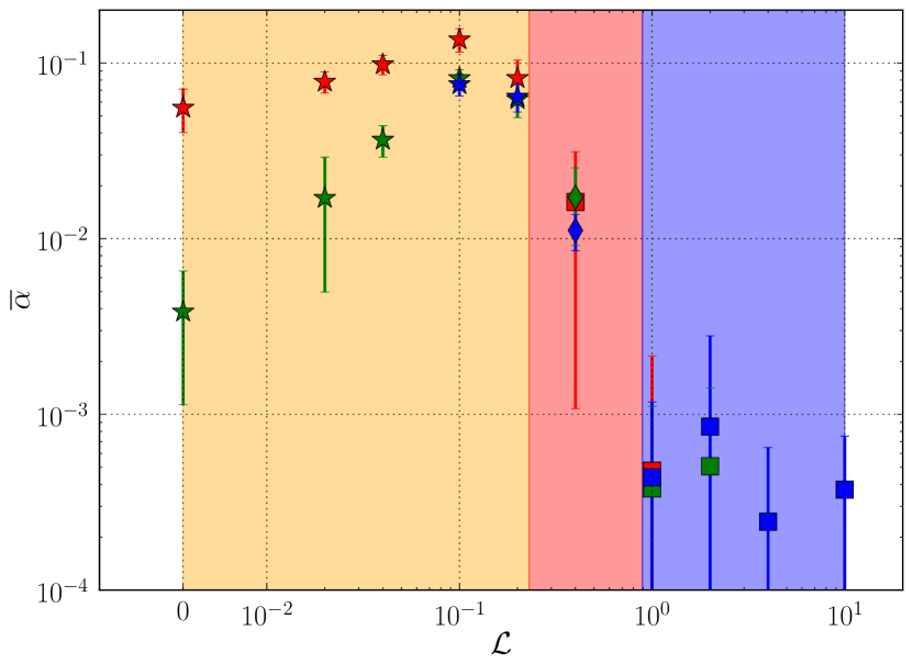
Figure 6: Time averaged total turbulent stress $\overline{\alpha}$ as a function of the Hall parameter $\mathcal{L}$ for runs B3 (red), B4 (green) and B5 (blue); the bars indicate the standard deviation over the averaging time interval; the final state of the flow is represented by stars for turbulence (filled orange region), diamonds for vortex (filled red region) and squares for zonal flows (filled blue region).

A significant fraction of mass is lost in these simulations: up to $50\%$ in run B3L3. The ratio of accreted to excreted mass is approximately $1$ in runs B3L0 to B3L2, increases to $1.8$ in B3L3, $1.5$ in B3L4, and decreases to $0.8$ in B3L5 and only $25\%$ in B3L6. In this last run, the excreted mass is transported by spiral density waves propagating through the entire domain, whereas turbulent accretion is totally suppressed. The same global trend is observed for all values of $B_{0}$. Despite this significant fraction of mass lost, imposing a constant mean magnetic field made it possible to reach quasi-steady states over several hundred inner orbits.

4.3 Zonal flows

4.3.1 Characterisation

We move our attention to the structural properties of the system, starting with Hall-induced zonal flows. As indicated in table 1, we find that the flow self-organises to long-lived axisymmetric structures whenever $\mathcal{L}\gtrsim 1$ (blue region in Fig. 6). At a given $\mathcal{L}$, the number of bands depends on the initially available magnetic flux, more flux producing a larger number of bands. Reciprocally, at a given $B_{0}$ the number of bands is found to increase with $\mathcal{L}$, the exception being run B5L7 where the flow instantaneously crystalized into three positive and negative magnetic field bands.

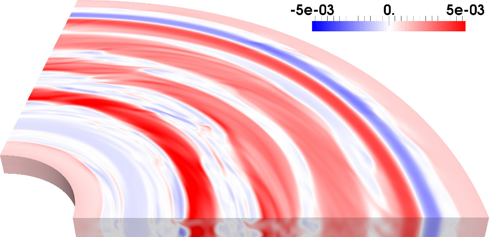
Figure 7: Vertical magnetic field in the run B3L6 at $t=300T_{0}$.

We show in Fig. 7 the state of run B3L6 at time $300T_{0}$. The vertical magnetic field appears to be organised in four axisymmetric bands, with little to no apparent vertical structure, and leaving the rest of the domain almost field-free.

4.3.2 Physical origin

The dynamics of these zonal fields or bands have been explored by KL13 and we recover here a similar qualitative picture. Let us first emphasize that the zonal field regions are dynamically stable. As demonstrated in Fig. 8, the vertical field strength in each band is so strong that it quenches the linear HSI. This fact explains why a stronger mean initial vertical flux leads to more bands of similar width. That being said, the bands having a limited radial extent, they should smear out radially because of diffusion (either numerical, physical or turbulent), reducing the field strength in the band and ultimately making the whole band HSI unstable again. This is not observed in our simulations and we find instead a confinement effect which calls for a proper explanation.

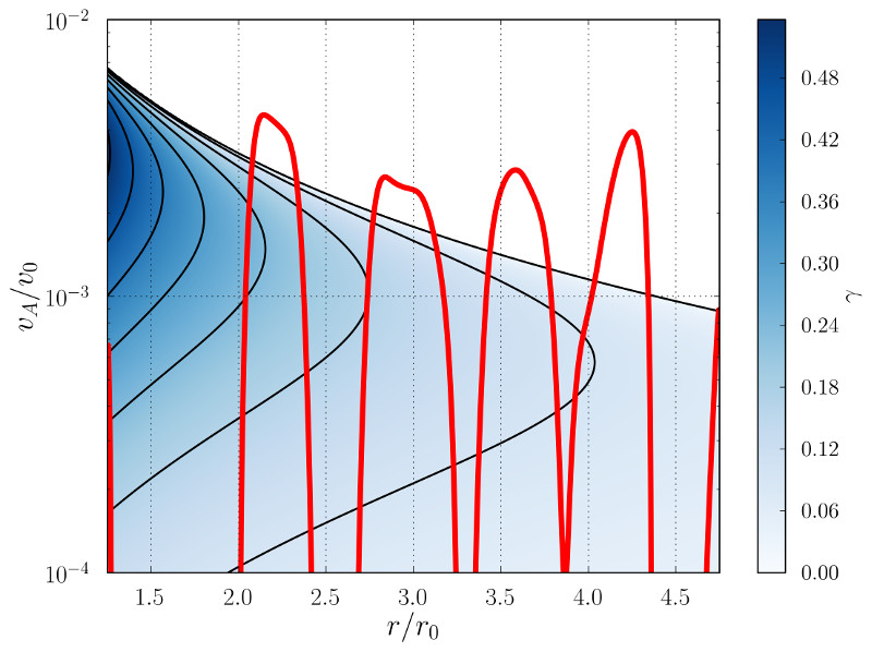
Figure 8: HSI linear growth rates for the mode with vertical wave vector $k_{z}=2\pi/h$ (blue color + contour lines), and local vertical Alfvén velocity (red) in run B3L6 averaged from $200T_{0}$ to $300T_{0}$.

The zonal field confinement takes its roots in the HSI at the boundary of each bands: the vertical flux is weaker but non-zero, allowing localised HSI modes to develop. This leads to the generation of a localised Maxwell stress at the border of each band, as illustrated in Fig. 9. However, in Hall-MHD, the Maxwell stress appears explicitly in the induction equation (9) through the Hall term. This equation predicts that a local maximum of the Maxwell stress pushes away positive vertical flux tubes. As a result, the growth of HSI modes at the border of each band pushes the vertical magnetic flux back in the band, thereby confining the flux in the HSI-stable region. This confinement mechanism by the Maxwell stress is sketched in Fig. 10 and explains the global organisation observed in these simulations.

The bifurcation to such a self-organised state from a fully turbulent state occurs when confinement overcomes diffusion. KL13 show from equation (9) that the transition happens near a critical $\mathcal{L}_{0}$ which depends on the stabilising Alfvén velocity (11) and on the turbulent magnetic Prandtl number $P_{m}\equiv\eta_{t}/\overline{\alpha}\Omega h^{2}$ via

$$\mathcal{L}_{0}\simeq\frac{1}{P_{m}}\frac{v_{A,\mathrm{crit}}}{\Omega h}.$$ (22)

Using $P_{m}\approx 2$ as measured in local simulations (Lesur & Longaretti, 2009), they deduce $\mathcal{L}_{0}\approx 0.2$. The same argument holds in our case, and the fact that the transition still happens near this critical value translates into a turbulent magnetic Prandtl number of order unity again in a global, non-stratified setup.

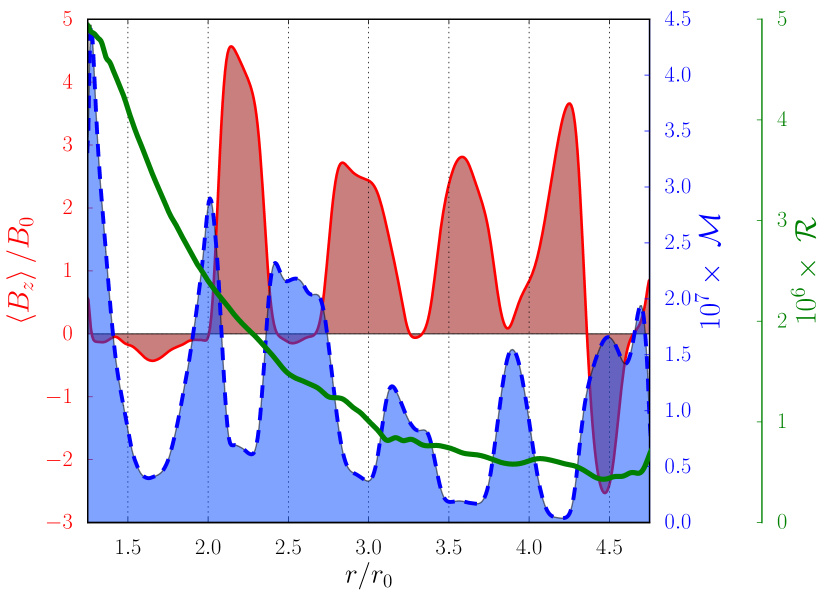
Figure 9: Radial profiles of $B_{z}$ (filled red), $10^{7}\times\mathcal{M}_{r\varphi}$ (dashed, filled blue) and $10^{6}\times\mathcal{R}_{r\varphi}$ (solid green) in run B3L6, averaged in time between $160T_{0}$ and $230T_{0}$.

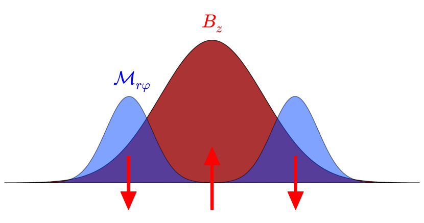
Figure 10: $B_{z}$ confinement mechanism by belts of Maxwell stress $\mathcal{M}_{r\varphi}$: the magnetic field decreases in regions of negative second derivative of $\mathcal{M}$, and increases where the curvature of $\mathcal{M}$ is positive.

Looking at the Reynolds component of the stress, we show in Fig. 9 that it is the dominant component of the total stress in this organised configuration, by a factor ten above the Maxwell stress. The physical origin of this stress resides in large-scale spiral waves, unaffected by the presence of zonal fields. We found a plateau of total stress when increasing $\mathcal{L}$ beyond unity although the Maxwell stress kept decreasing below $\overline{\alpha_{\mathcal{M}}}<10^{-4}$ near the end of the simulation. After ruling out a possible defect of our inner damping regions, we think these waves may be excited by residual turbulence and local minima of potential vorticity near the zonal flows.

4.4 Vortices

4.4.1 Characterisation

For intermediate Hall strengths, the level of turbulent stress remains quite high but the aspect of the turbulent structures gets more clumpy as $\mathcal{L}$ is increased (red region in Fig. 6). We quantify this structural transition in Fig. 11, with the median value (over the radial extent of the disk) of the normalized correlation lengths of $\delta B_{z}\equiv B_{z}-B_{0}$ in the vertical and azimuthal directions. The change from small to large-scale fluctuations occurs rapidly for $\mathcal{L}\gtrsim 0.2$, and when $\mathcal{L}\geq 1$ the correlation factor is stalled near unity.

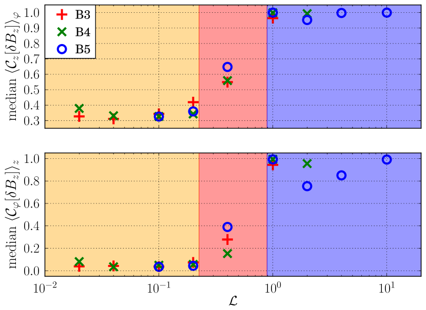
Figure 11: Median value of the vertical (upper panel) and azimuthal (lower panel) auto-correlation profiles of the vertical magnetic field $\delta B_{z}$, measured at the end of the quarter-disk runs B3 (red plus), B4 (green cross) and B5 (blue circles); the orange, red and blue regions correspond respectively to a turbulent, vortex and zonal flow final state.

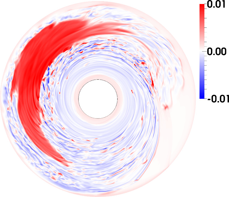
Figure 12: Vertical magnetic field in run 2$\pi$L5 at time $300T_{0}$.

During the transition $\mathcal{L}\approx 0.4$, the turbulent fluctuations merge to form a sustained patch of magnetic field in runs B4L5 and B5L5. One band was formed in run B3L5 with the same $\mathcal{L}$; Fig. 6 shows that it is affected by large fluctuations in stress over time, indicating that the structure is not steady. In order to test its stability, we ran the full-disk simulation 2$\pi$L5 and found that the band would actually break and rather form a large patch as illustrated in Fig. 12. In this run the average vertical field is $B_{z}\approx 8\times 10^{-3}$ inside the patch. Similarly to the zonal flows of section 4.3, this region displays no structure in the vertical direction. We verified that these magnetic islands were not a mere product of the global flux adjustment procedure (see 3.1.2). These large scale patches have not been observed in KL13 local simulations probably because their horizontal extension covers several geometrical scale height $h$ in radius and azimuth. For larger $\mathcal{L}\gtrsim 1$, the bands are stable in the full-disk configuration as confirmed in run 2$\pi$L6. The formation of a band in run B3L5 is facilitated by the smaller angular extent of the domain, and therefore accidental. We also confirm with run 2$\pi$L4 that lower values for $\mathcal{L}\lesssim 0.2$ keep the flow turbulent in $2\pi$ disk simulations.

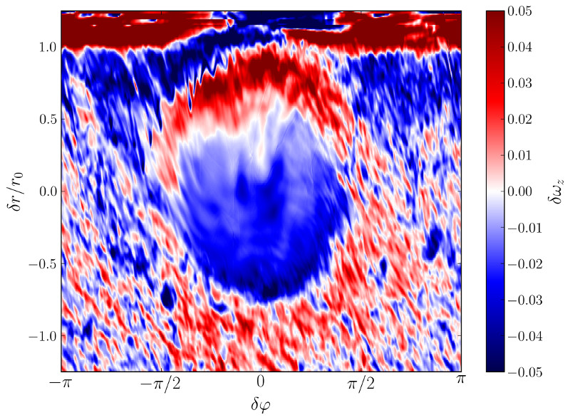
Figure 13: Vertical vorticity fluctuation $\delta\omega_{z}$ in the $\left(\varphi,r\right)$ plane of run 2$\pi$L5, centered on the vortex, averaged in the vertical direction and in time with five snapshots between $250T_{0}$ and $290T_{0}$; the vertical axis $\delta r/r_{0}$ is the radial distance to the measured center of the vortex.

In the limit of incompressible Hall-MHD, the canonical vorticity

$$\bm{\varpi}\equiv\nabla\times\bm{v}+\bm{B}/\rho\ell_{\mathrm{H}}$$ (23)

is a conserved quantity (see equation 7 of KL13); an increase in magnetic flux therefore comes with a decrease in vorticity flux. We show in Fig. 13 the vertical component of the vorticity fluctuation from the initial keplerian flow: $\delta\bm{\omega}\equiv\nabla\times(\bm{v}-r^{-1/2}\bm{e_{\varphi}})$, averaged in time over $40$ inner orbits for better discernibility. We observe that the accumulation of magnetic flux is indeed balanced by a decrease in vorticity flux: $\delta\omega_{z}\simeq-\delta B_{z}/\rho\ell_{\mathrm{H}}\approx 3\times 10^{-2}$, making this patch a true vortex and attesting the role of the Hall effect in its formation. Its center is localised near $3.8r_{0}$, and the ratio of its major to minor axis is $\chi\approx 5.2$; the corresponding proper rotation period is

$$\delta t\simeq\frac{2\pi}{\delta\omega_{z}}\frac{1+\chi^{2}}{\chi}\approx 180T_{0},$$ (24)

or approximately $25$ local orbits. This turn-over time is large compared to the local dynamical time-scale, which is why our time averages suffer from random fluctuations.

4.4.2 Confinement mechanism

The radial confinement of the vortex obeys the same mechanism as for the zonal flows; we can address it with a one-dimensional approach similar to the axisymmetric model of section 2.2. In the case of zonal flows, a band of magnetic field is pushed from both its inner and outer sides by the $(r,\varphi)$ component of the Maxwell stress $\mathcal{M}_{r\varphi}$, which is the product of the magnetic field component along the streamlines $B_{\varphi}$ with the component perpendicular to the streamlines $-B_{r}$. A vortex is defined by closed streamlines, dragging and wrapping the horizontal magnetic field around. In a frame following the vortex at its local keplerian velocity, one can use the magnetic field components along ($B_{\parallel}$) and perpendicular ($-B_{\perp}$) to the velocity streamlines. The product of these components defines a projected Maxwell stress $\mathcal{M}_{\perp\parallel}$; this stress appears at the boundary of the magnetic patch and pushes magnetic flux in the perpendicular direction $-\bm{e_{\perp}}$, thus confining the vortex from all directions.

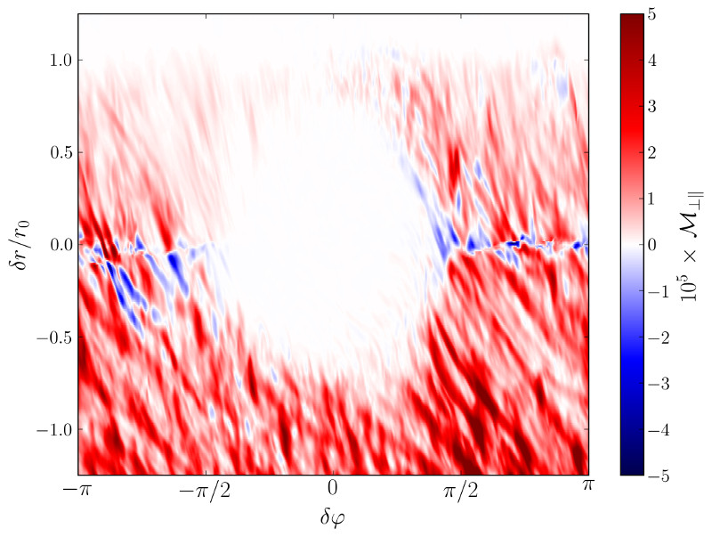
Figure 14: Projected stress in the $\left(\varphi,r\right)$ plane of run 2$\pi$L5, centered on the vortex, averaged in the vertical direction and in time with five snapshots between $250T_{0}$ and $290T_{0}$; the vertical axis $\delta r/r_{0}$ is the radial distance to the measured center of the vortex.

We confirm this picture by showing the averaged map of projected Maxwell stress $\mathcal{M}_{\perp\parallel}$ of run 2$\pi$L5 in Fig. 14. We find that it is negligibly small inside the vortex, attesting of the MHD stability of this region, while the overall positive stress around the vortex provides the required confinement.

5 Dust trapping

An important issue is the ability of the previous structures to accumulate dust particles in the process of planetary formation. It is known that, due to aerodynamic drag, dust grains migrate outwards in super-keplerian regions and migrate inwards in sub-keplerian regions (Weidenschilling, 1977). A disc region trapped between a super-keplerian part at its inner side and a sub-keplerian part at its outer side therefore constitute a dust trap where dust grains accumulate.

In the incompressible Hall-MHD limit, an increase in magnetic flux should come with a decrease in vorticity flux, so that the flux of canonical vorticity defined by equation (23) is conserved. This is equivalent to a velocity profile steepened in regions of accumulated magnetic field and flattened outside, making both zonal flows and vortices potential dust traps.

5.1 Capture by zonal flows

To see how the conservation of the canonical vorticity flux is altered in our compressible case, we draw in Fig. 15 the deviation from a keplerian rotation profile in run B3L6. We observe a transition from super to sub-keplerian rotation speed only in the first two bands. In the outer half, the initially turbulent state plus the steady mass excretion by spiral waves have reduced the average density to about $10\%$ of its initial value and slightly increased it in the center of the radial domain; this global density (and therefore pressure) gradient is sufficient to maintain a sub-keplerian flow in the outer part of the disk, preventing dust trapping in the last two bands.

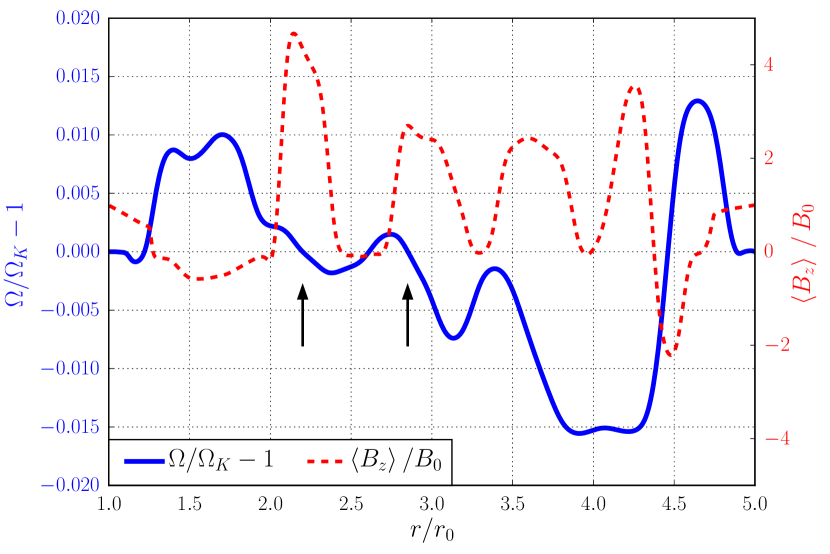
Figure 15: Relative fluctuations of angular velocity (solid blue) and vertical magnetic field (dashed red) in run B3L6, averaged in time between $260T_{0}$ and $300T_{0}$. The arrows indicate regions of favored dust accumulation.

In general, protoplanetary disks are expected to be globally sub-keplerian thanks to a mean negative pressure gradient. This deviation from keplerian rotation can be computed by considering the radial equilibrium

$$\frac{\Omega}{\Omega_{K}}=\Bigg{(}1+\frac{\partial_{r}P}{\rho R\Omega_{K}^{2}}\Bigg{)}^{1/2}.$$ (25)

The average pressure gradient entering this equation can be estimated from the aspect ratio of the disk $\varepsilon=c_{s}/R\Omega_{K}$ so that one expects

$$\frac{\Omega}{\Omega_{K}}-1\simeq-\frac{1}{2}\varepsilon^{2}.$$ (26)

Assuming a typical value of $\varepsilon=0.1$, we find that the deviations to Keplerian rotation driven by our zonal flows in Fig. 15 are marginally sufficient to create super-keplerian regions (and thus dust traps) when this mean pressure gradient is included. For this reason, we expect that only a few of these zonal flows (the strongest ones) can trap dust in models including a realistic mean pressure gradient.

5.2 Capture by vortices

The possible role of hydrodynamic vortices as dust traps in protoplanetary disks was highlighted by Barge & Sommeria (1995) and Tanga et al. (1996), and has now received both analytical and numerical investigations (e.g. Johansen et al., 2004; Chavanis, 2000) . We focus on the necessary condition for a vortex to be a dust trap: that it is over-pressured with respect to the surrounding flow (see footnote 2). In our globally isothermal simulations, this translates into an over-density in the vortex.

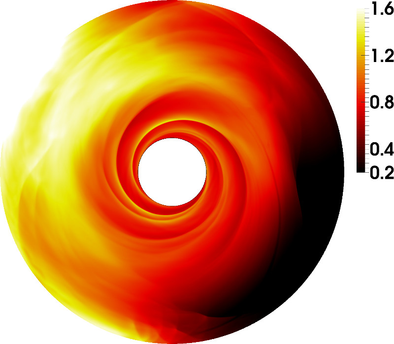
Figure 16: Density distribution in run 2$\pi$L5 at time $300T_{0}$.

We show in Fig. 16 a snapshot of the density distribution in run 2$\pi$L5 at time $300T_{0}$. Comparing with Fig. 12, there is clearly an over-density at the location of the vortex, with mean value $1.5\rho_{0}$ inside at $300T_{0}$, so this vortex would be able to trap dust particles.

6 Threats to self-organisation

The simulations presented so far were done in the Hall MHD regime with an imposed mean vertical magnetic field. However, stratified shearing box models (e.g. Lesur et al., 2014) also indicate that the magnetic field could be essentially toroidal in the midplane of protoplanetary disks, which could in turn affect the formation and stability of zonal flows. Besides, ionisation models (e.g. Simon et al., 2015) suggest that the Hall effect is dominant only in intermediate regions ($1\,\mathrm{a.u.}\lesssim r\lesssim 30\,\mathrm{a.u.}$) of protoplanetary disks, the inner and outer region being respectively dominated by Ohmic and ambipolar diffusion (Turner et al., 2014). These diffusive processes could prevent the formation of sharp magnetic accumulations. We investigate the robustness of our previous findings against these effects in the three next sections.

6.1 Toroidal field

6.1.1 Method

We ran eight simulations where both the vertical and azimuthal magnetic fluxes are imposed and adjusted at every timestep. As before, we let a disk evolve over $50T_{0}$ from a keplerian flow with initial magnetic field $\bm{B}=B_{0}\bm{e_{z}}+B_{\varphi}\bm{e_{\varphi}}$ to a fully turbulent flow, where $B_{0}=B_{\varphi}=10^{-3}$ initially constant over the whole domain. This choice of initial conditions does not correspond to an MHD equilibrium, but the intensity of the magnetic field is weak enough to reach a steady turbulence in an overall keplerian flow. We activated the Hall effect from this starting point in all eight runs, and lowered the average vertical magnetic field to $B_{0}=10^{-4}$ for half of them, keeping $B_{\varphi}=10^{-3}$. The stopping time is set to $300T_{0}$ for runs T3L3 and T4L2, and to $200T_{0}$ for the others. The parameters of these runs are given in Table 2.

6.1.2 Results

Simulations with net vertical and toroidal magnetic flux Name $B_{0}$ $\mathcal{L}$ $\overline{\alpha}$ state T3L0 $10^{-3}$ $0$ $6.2\times 10^{-2}$ turbulent T3L1 $10^{-3}$ $0.1$ $1.4\times 10^{-1}$ turbulent T3L2 $10^{-3}$ $0.4$ $1.0\times 10^{-2}$ vortex T3L3 $10^{-3}$ $1$ $1.1\times 10^{-3}$ 3 bands T4L0 $10^{-4}$ $0$ $4.9\times 10^{-3}$ turbulent T4L1 $10^{-4}$ $0.1$ $7.9\times 10^{-2}$ turbulent T4L2 $10^{-4}$ $0.4$ $7.3\times 10^{-3}$ turbulent T4L3 $10^{-4}$ $1$ $3.3\times 10^{-3}$ 1 band

Table 2: Parameters for the 3D Hall MHD runs with toroidal field: label of the run, mean vertical magnetic field $B_{0}$, Hall parameter $\mathcal{L}$, total averaged turbulent stress $\overline{\alpha}$ and final state.

From the last column of Table 2, we notice minor differences in the final state of these simulation compared to the case of a purely vertical mean field: run T3L3 produced 3 bands instead of 4, and run T4L2 did not produce a distinct vortex but only short-lived patchy magnetic islands.

We then compare the average stress in these toroidal runs with the previous vertical ones in Fig. 17. The addition of a toroidal magnetic field is seen to have no significant impact on the stress. In particular, the transition from high to low transport states near $\mathcal{L}\approx 0.1$ is preserved. Only the run T4L3 shows a turbulent stress significantly higher than the analogue run with zero net toroidal flux. This stress comes essentially from the Reynolds component: in all the runs with $\mathcal{L}=1$ the Maxwell stress kept decreasing below $\overline{\alpha_{\mathcal{M}}}<10^{-4}$ at the end of the simulation, but since the Reynolds stress was statistically steady at a much higher values we did not prolong these runs further.

These differences attest the presence of a slightly stronger turbulent activity, able to weaken magnetic structuring but not drastically changing the picture.

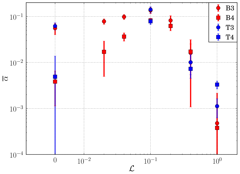
Figure 17: Time-averaged stress $\overline{\alpha}$ as a function of the Hall parameter $\mathcal{L}$, with and without a toroidal field (blue and red respectively), with mean vertical field $B_{0}=10^{-3}$ (circles) and $B_{0}=10^{-4}$ (squares); the bars represent standard deviations of $\left\langle\alpha\right\rangle$ over time.

6.2 Ohmic diffusion

6.2.1 Linear stability

The presence of ohmic resistivity narrows the range of accessible HSI modes. In the strong Hall limit, the marginal stability of axisymmetric Hall-shear modes with wave vector $k$ in a background vertical field requires (Balbus & Terquem, 2001) :

$$\ell_{\mathrm{H}}v_{A}\left(\ell_{\mathrm{H}}v_{A}k^{2}-q\Omega\right)+\eta_{\mathrm{O}}^{2}k^{2}=0.$$ (27)

The addition of resistivity affects the two bounds between which instability occurs :

$$\frac{2\ell_{\mathrm{H}}v_{A}k^{2}}{q\Omega}=1\pm\sqrt{1-\left(\frac{2\eta_{\mathrm{O}}k^{2}}{q\Omega}\right)^{2}}.$$ (28)

In order to study self-organisation, the system must initially be between these two bounds. A minimum magnetic field intensity is necessary for linear instability and the possibility of sustaining turbulence. In the other limit, the field intensity required to damp the largest scales $k_{0}=2\pi/h$ is lowered by diffusivity, which may help the formation of Hall-shear stable regions and favor self-organisation. We tune this range of unstable magnetic fields with the magnetic Reynolds number $\mathcal{R}_{\mathrm{O}}\equiv q\Omega/2\eta_{\mathrm{O}}k_{0}^{2}$.

6.2.2 Method

The numerical setup used in this section is the same as in section 4, but with a constant resistivity $\eta_{\mathrm{O}}$ in the active domain (and always the resistivity $\eta_{b}$ in the damping buffer zones). We sampled two values of magnetic Lundquist numbers $\mathcal{S}_{\mathrm{O}}=\{2.5,25\}$, and the magnetic Reynolds number $\mathcal{R}_{\mathrm{O}}$ is appreciably close to unity only in the small $\mathcal{S}_{\mathrm{O}}=2.5$ case. These values should be sufficiently low to produce observable effects in our runs, but not prevent self-organisation by immediately damping any perturbation. All four runs are integrated in time from $50T_{0}$ to $200T_{0}$.

6.2.3 Results

Simulations with ohmic diffusion
Name $B_{0}$ $\mathcal{S}_{\mathrm{O}}\>(\mathcal{R}_{\mathrm{O}})$ $\mathcal{L}$ $\overline{\alpha}$ state O3N0 $10^{-3}$ $25\>(119\Omega)$ $0.4$ $1.2\times 10^{-2}$ vortex O3N1 $10^{-3}$ $25\>(119\Omega)$ $1$ $5.2\times 10^{-4}$ 2 bands O3N2 $10^{-3}$ $2.5\>(12\Omega)$ $1$ $1.2\times 10^{-3}$ 1 band O4N3 $10^{-4}$ $2.5\>(119\Omega)$ $1$ $9.6\times 10^{-4}$ 1 band

Table 3: Parameters for the 3D Hall+Ohm MHD runs with toroidal field: label of the run, mean vertical magnetic field $B_{0}$, magnetic Lundquist numbers $\mathcal{S}_{\mathrm{O}}$ and corresponding Reynolds number $\mathcal{R}_{\mathrm{O}}$, Hall parameter $\mathcal{L}$, turbulent stress $\overline{\alpha}$ and final state of the flow.

We see in Table 3 that resistivity does affect the number of zonal flows produced in our simulations: two in O3N1 and one in O3N2, instead of four in the $\eta_{\mathrm{O}}=0$ case of run B3L6. However, the outcome of runs O3N0 and O4N1 is the same as their non-resistive versions: a vortex in the former case, and one band in the latter.

It is worth noting that from run O3N1 to O3N2, increasing the resistivity by a factor ten resulted in an increase of Maxwell stress by a factor two. Similarly, the total stress is twice higher in O4N3 than in the non-resistive equivalent scenario B4L6. This behavior comes from the diffusive broadening of the bands, leaving a wider region linearly unstable at their edges and maintaining a larger fraction of the domain unstable to the MRI.

We thus find that for magnetic Lundquist numbers $\mathcal{S}_{\mathrm{O}}\gtrsim 1$, ohmic diffusion can reduce the number of zonal flows, but the system keeps self-organising. A similar final state is obtained when resuming the organised run B3L6 with resistivity: diffusion overcomes concentration between the bands and allows them to merge. The fact that a band remains at the end of the simulation suggests that this merging process is halted once the bands are too far to share magnetic flux. At this point, ohmic diffusion adds to turbulent diffusion in equation (9), balancing the confinement by Maxwell stress.

6.3 Ambipolar diffusion

We finally look at the impact of ambipolar diffusion on self-organisation. With its non-linear dependence on $B$, this effect may lead to more complex behaviours than ohmic diffusion. The region of protoplanetary disks dynamically affected by ambipolar diffusion is expected to overlap the Hall dominated region, with typical ambipolar Elsasser numbers $\Lambda_{\mathrm{A}}$ below unity (Simon et al., 2015). We first test the robustness of Hall self-organisation against ambipolar diffusion; we then turn our attention to a configuration in which Bai & Stone (2014) report self-organisation without the Hall effect, and compare it to our Hall-dominated simulations.

As previously, we activate ambipolar diffusion and the Hall effect simultaneously at $50T_{0}$ and integrate until $200T_{0}$, with various values for the global magnetic flux, the ambipolar Lundquist number $\mathcal{S}_{\mathrm{A}}$ via the ratio $\eta_{\mathrm{A}}/v_{A}^{2}$, and the Hall parameter. The ambipolar Lundquist numbers are similar to the ohmic Lundquist numbers of the previous section, and the corresponding Elsasser numbers range from $0.01$ to $1$.

6.3.1 Hall+Ambipolar MHD

Simulations with ambipolar diffusion
Name $10^{4}B_{0}$ $\mathcal{S}_{\mathrm{A}}\>(\Lambda_{\mathrm{A}}^{0})$ $\mathcal{L}$ $\overline{\alpha}$ state A3N0 $10$ $25\>(0.1)$ $1$ $1.0\times 10^{-3}$ 2 bands A3N1 $10$ $25\>(0.1)$ $2$ $1.1\times 10^{-3}$ 3 bands A3N2 $10$ $2.5\>(0.01)$ $1$ $7.3\times 10^{-4}$ 2 bands A3N3 $10$ $2.5\>(0.01)$ $0.4$ $9.6\times 10^{-4}$ 2 bands A3N4 $10$ $2.5\>(0.01)$ $0.2$ $1.5\times 10^{-3}$ 2 bands A4N5 $1$ $25\>(0.01)$ $1$ $1.3\times 10^{-3}$ channel A4N6 $1$ $25\>(0.01)$ $4$ $1.1\times 10^{-3}$ 3 bands ABS $18$ $139\Omega\>(1)$ $0$ $4.2\times 10^{-3}$ turbulent

Table 4: Parameters for the 3D Hall+Ambipolar MHD runs: label of the run, mean vertical magnetic field $B_{0}$, ambipolar Lundquist number $\mathcal{S}_{\mathrm{A}}$, corresponding ambipolar Elsasser number $\Lambda_{\mathrm{A}}^{0}$ at the inner radius $r_{0}=1$, Hall parameters $\mathcal{L}$, total turbulent stress $\overline{\alpha}$ and final state of the flow; “channel” describes a computational domain filled with linear HSI modes; only run ABS has a diffusivity scaling as $r^{3/2}$, corresponding to a constant ambipolar Elsasser number $\Lambda_{\mathrm{A}}=1$.

We see in Table 4 that the total turbulent stress is not significantly affected by ambipolar diffusion in the low-transport state, the magnetic contribution still being negligibly small. Compared to the non-diffusive case, we find a smaller number of zonal flows with ambipolar diffusion in runs A3N0 to A3N2, but it is larger than the case of an equivalent ohmic Lundquist number (see Table 3). An inefficient merging of magnetic bands may be explained by the fact that ambipolar diffusion has little influence in the field-free region between the bands.

When lowering the average magnetic flux in run A4N5, we obtain a disk filled with global channel modes and no zonal field. Since the average magnetic field is far below the threshold for HSI stabilisation, linear modes develop until the ambipolar diffusive damping rate, of order $\eta_{\mathrm{A}}/h^{2}$, balances their growth rate. The resulting stress has an almost flat radial profile, providing no confinement at the scale of our computational domain. Run A4N6 proves that when increasing $\mathcal{L}$ at the same field intensity, the Hall effect becomes competitive again and we recover several zonal fields.

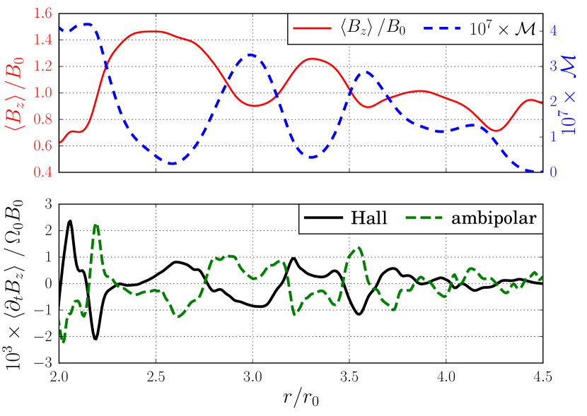
Figure 18: Radial profiles in run A3N4, averaged in the vertical and azimuthal directions, and in time between $150T_{0}$ and $250T_{0}$. Upper panel: vertical magnetic field (solid red) and Maxwell stress (dashed blue); lower panel: contributions of the Hall (solid black) and ambipolar (dashed green) drifts to the induction of vertical magnetic field $\partial_{t}B_{z}$.

A new feature is the possibility of forming zonal fields at lower $\mathcal{L}<1$, as demonstrated by runs A3N3 and A3N4. We show in Fig. 18 the radial profile of vertical magnetic field in run A3N4, and the contributions of both non-ideal effects to the induction equation (3) in the vertical direction. The variations of $B_{z}$ have a much smaller amplitude than in Hall-only runs (see Fig. 9), but they still show a clear anti-correlation with the variations of Maxwell stress. As previously, we find that the Hall effect tries to increase $B_{z}$ in the bands and decrease it between. The ambipolar drift does precisely the opposite: it tries to smooth out the profile of $B_{z}$, and both contributions appear to cancel out on average.

Since the Hall effect now balances ambipolar rather than turbulent diffusion, the self-organisation threshold given by (22) needs not hold anymore. Ambipolar diffusion acts to damp fluctuations in magnetic field, so the turbulent diffusivity $\eta_{t}$ entering equation (9) must eventually decrease when the ambipolar diffusivity is increased. In the limit of strong ambipolar diffusion, the bifurcation to a self-organised state should depend on $\eta_{\mathrm{A}}$ only. The fact that we observe two bands at $\mathcal{L}=0.2$ may result from an effective diffusivity $\eta_{t}+\eta_{\mathrm{A}}$ smaller than in the Hall-only case, due to the decrease of $\eta_{t}$ as a function of $\eta_{\mathrm{A}}$.

We conclude that self-organisation holds for ambipolar Elsasser numbers down to $\Lambda_{\mathrm{A}}=0.01$, and that ambipolar diffusion can enable the formation of zonal flows for $\mathcal{L}$ as low as $0.2$.

6.3.2 Self-organisation with ambipolar diffusion only

Magnetic self-organisation was also reported by Bai & Stone (2014) in local simulations of MRI turbulent flows without the Hall effect; since ambipolar diffusion was found to enhance magnetic flux concentration, we included this non-ideal effect only and tried to reproduce the physical conditions of their run AD-4-64 within our global setup in run ABS. The initial magnetic field is set to $B_{0}=\sqrt{2c^{2}\rho_{0}/6400}\approx 1.8\times 10^{-3}$, and the ambipolar Elsasser number $\Lambda_{\mathrm{A}}=1$ is constant throughout the computational domain, so that both setups should match at the inner boundary. Considering the narrowness of the magnetic structures observed by Bai & Stone (2014), we used the HLLD approximate Riemann solver to reduce numerical diffusivity in this run only.

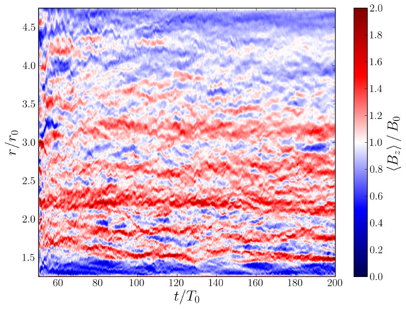
Figure 19: Normalized vertical magnetic field $\left\langle B_{z}\right\rangle/B_{0}$ in run ABS.

In comparison to their figure 7, we confirm in our Fig. 19 that the vertical magnetic flux does concentrate into bands. They are most clearly visible in the inner half of the disk, where they live a few tens of orbits before being disrupted and formed again in the turbulent flow. Averaging this profile in time, we find mean fluctuations of about $0.3B_{0}$ revealing five bands at radii $1.5$, $1.9$, $2.2$, $2.6$ and $3.2r_{0}$. We note a broadening of these bands with radius, suggesting some self-similar scaling $\lambda^{2}\sim\tilde{\eta}/\Omega$ of the characteristic concentration length-scale $\lambda$ with the local time-scale for some effective anti-diffusivity $\tilde{\eta}$, and not a constant concentration length of order $h$ as for the Hall effect.

We show in Fig. 20 the correlation profiles of $\delta B_{z}$ in run ABS at time $200T_{0}$. The median values are $0.3$ and $0.08$ for the vertical and azimuthal correlation lengths respectively, with peak values up to $0.5$ in azimuthal correlation at the location of each spotted band. These median values are consistent with those from a fully turbulent state (see Fig. 11). In particular there is no strong vertical coherence in the bands, confirming that these magnetic concentrations can never stabilize the flow in the full height of the disk; in comparison, the zonal fields produced by the Hall effect are always Hall-shear stable with vertical correlation factors close to unity.

We conclude that the self-organisation process observed by Bai & Stone (2014) is fundamentally different from the Hall-induced self-organisation mechanism presented in this paper.

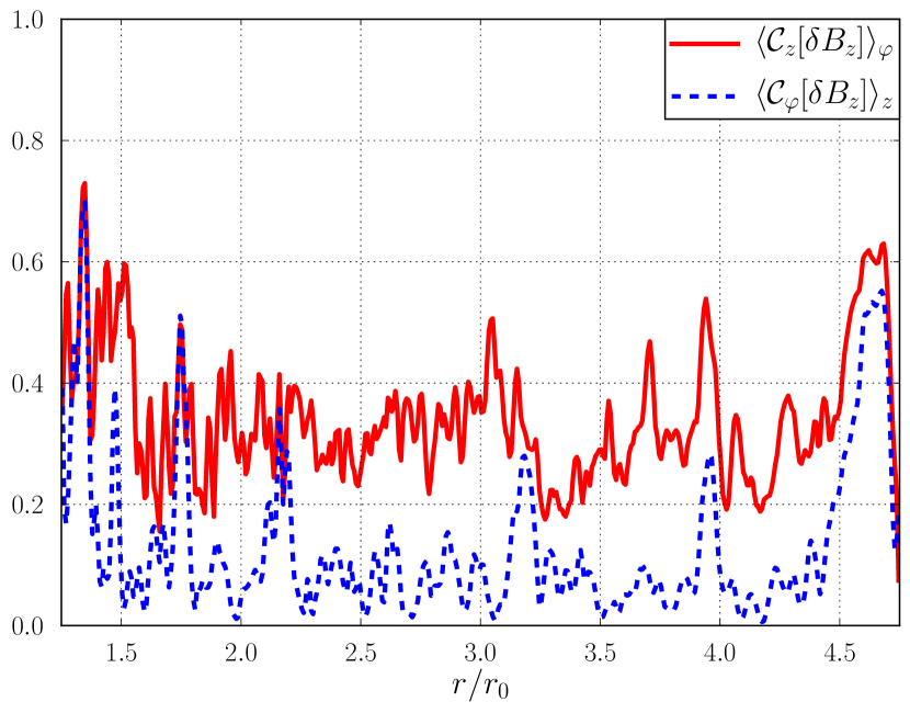
Figure 20: Radial profiles of averaged vertical (solid red) and azimuthal (dashed blue) correlations lengths for the fluctuation in vertical magnetic field $\delta B_{z}$ in run ABS at time $200T_{0}$.

7 Summary and discussion

We have presented a number of non-ideal MHD simulations dedicated to the Hall dominated regions of protoplanetary disks. We employed a global non-stratified model designed to naturally extend results from local shearing box simulations. For this purpose, we have extended the PLUTO code in order to include the Hall effect in cylindrical geometry, and validated our implementation in the linear regime of the resistive MRI. We then performed a series of global Hall-MHD simulations, focusing on the different stages of self-organisation found as the intensity of the Hall effect is increased. Finally, we addressed the consequences of a net toroidal magnetic flux, as well as ohmic or ambipolar diffusion, on this picture of Hall-induced self-organisation.

We can summarise our main findings as follow:

1. We confirm the transition from enhanced to lowered turbulent transport states when increasing the intensity of the Hall effect; the turning point is found at $\mathcal{L}\approx 0.1$, comparable to the estimate of KL13.

2. In the strong Hall limit $\mathcal{L}\gtrsim 1$, self-organisation leads to the formation of stationary zonal flows in cylindrical geometry; as the Hall length or the available magnetic flux is increased, so does the number of zonal flows, until the computational domain is filled with bands of accumulated magnetic field with typical width $h$.

3. When increasing $\mathcal{L}$ from zero, the transition from a small-scale turbulence to axisymmetric zonal flows is accompanied by the formation of large-scale magnetised vortices, a feature barely accessible in local simulations for it requires a large aspect ratio in the radial over vertical directions.

4. Both the vortices and the zonal flows caused by the Hall effect may play a role in the process of planetary formation, since they can affect the rotation profile of the gas sufficiently to trap dust particles.

5. The self-organisation mechanism described in this paper holds when including a net toroidal field, ohmic or ambipolar diffusion; both diffusive effects cause the magnetic structures to merge over time, but do not change significantly the total torque exerted on the disk; ambipolar diffusion is found to enable self-organisation at lower Hall parameter $\mathcal{L}$.

These results demonstrates that Hall-MRI is a very promising mechanism through which large scale structures can form and be observed. One should however keep in mind that these simulations are still very simplified and leave many questions opened. First, we have entirely neglected vertical stratification and we have simplified the radial structure to keep relatively constant diffusion parameters. Vertical stratification can be very important as it drives surface winds and accretion thanks to magnetic torques. Stratified shearing box models including the Hall effect have not shown any obvious self-organisation, but this is likely due to the limited radial extension of these boxes. The mechanism we propose for the self organisation is relatively simple and robust as it only relies on 3 hypotheses: 1- the disc is sufficiently ionised to be MRI/HSI unstable, 2- the $r-\phi$ component of the Maxwell stress vanishes for strong enough field strengths and 3- the Hall length-scale is of the order of the disc scale height. Hypotheses 1 and 3 are usually satisfied in the midplane of stratified models. However, hypothesis 2 can be violated when a strong large scale wind is present, as the Maxwell stress is not only due to local physics but also to the global wind dynamics. Testing self-organisation in global stratified models is therefore essential to confirm this picture.

It is also worth pointing out that several of our simulations exhibit stable magnetised vortices. This might look surprising as vortices are known to be strongly unstable in magnetised discs due to magneto-elliptic instabilities (Mizerski & Bajer, 2009). We have not investigated extensively the stability of these objects, but the presence of a strong field in the vortex core is most certainly the key to their stability, as this tends to rigidify flow motions and prevent fluid particles from entering into a resonance with the vortex turnover frequency.

Whether the structures produced in our simulations can be observed is yet another opened question. It is clear that some of these structures are dust traps, and should therefore accumulate millimetre-sized dust particles. However, this dust might also react on the flow, and even affect the ionisation structure, thereby changing the dynamics. This complex interplay between MHD, dust and chemistry have not been included in our models for obvious simplification reasons, but this step will be required if one is to predict the dust density contrast in rings and vortices and predict observational properties of these features.

Appendix A Spectral method for linear non-ideal MHD in axisymmetric configuration

We start with the full set of equations describing a magnetised fluid in non-ideal compressible magnetohydrodynamics:

$$\partial_{t}\rho+\bm{\nabla\cdot}\left[\rho\bm{v}\right] =0$$ (29)

$$\rho\left(\partial_{t}\bm{v}+\bm{v\cdot\nabla v}\right) =-\bm{\nabla}P+\bm{J\times B}+\upsilon\bm{\Delta}\bm{v}-\rho\bm{\nabla}\Phi$$ (30)

$$\begin{split}\partial_{t}\bm{B}&=\bm{\nabla\times}\left[\bm{v\times B}-\eta\bm{\nabla\times B}\right.\\ &\left.-\ell_{\mathrm{H}}\left(\bm{\nabla\times B}\right)\bm{\times B}+\gamma\left(\left(\bm{\nabla\times B}\right)\bm{\times B}\right)\bm{\times B}\right]\end{split}$$ (31)

completed by the closures $\bm{J}=\nabla\times\bm{B}$ and $P=c_{s}^{2}\rho$ where $\rho$ is the fluid density, $\bm{v}$ is its velocity, $\bm{B}$ the magnetic field, $P$ the pressure, $\bm{J}$ the electric current density, $\eta$ the ohmic diffusivity, $\upsilon$ the kinematic viscosity, $\ell_{\mathrm{H}}$ the Hall length and $\gamma$ the ambipolar diffusion coefficient. $\Phi$ is a gravitational potential $\propto r^{-1}$ in cylindrical coordinates $(r,\varphi,z)$.

These equations are linearized about the stationary solution $\bar{\rho}=\rho_{0}$, $\bar{B}=B_{0}e_{z}$, $\bar{v}=\Omega re_{\varphi}$ where $\Omega(r)\propto r^{q}$ and $q=-3/2$ in the keplerian case. We restrict ourselves to axisymmetric perturbations: $\partial_{\varphi}=0$. Defining $D_{r}\equiv\frac{1}{r}+\partial_{r}$, the equation for the perturbed density reads

$$\partial_{t}\rho^{\prime}=-\rho_{0}\left(D_{r}v^{\prime}_{r}+\partial_{z}v^{\prime}_{z}\right),$$ (32)

and the perturbed velocity:

$$\begin{split}\partial_{t}v^{\prime}_{r}&=-\frac{c_{s}^{2}}{\rho_{0}}\partial_{r}\rho^{\prime}+\upsilon\left(\partial_{r}^{2}+\frac{1}{r}\partial_{r}\right)\left[v^{\prime}_{r}\right]\\ &+2\Omega v^{\prime}_{\varphi}+\frac{B_{0}}{\rho_{0}}\left(\partial_{z}B^{\prime}_{r}-\partial_{r}B^{\prime}_{z}\right)\end{split}$$ (33)

$$\partial_{t}v^{\prime}_{\varphi} =-\left(2+q\right)\Omega v^{\prime}_{r}+\frac{B_{0}}{\rho_{0}}\partial_{z}B^{\prime}_{\varphi}$$ (34)

$$\partial_{t}v^{\prime}_{z} =-\frac{c_{s}^{2}}{\rho_{0}}\partial_{z}\rho^{\prime}+\upsilon\partial_{z}^{2}v^{\prime}_{z}$$ (35)

Finally for the perturbed magnetic field:

$$\begin{split}\partial_{t}\bm{B^{\prime}}&=\bm{\nabla\times}\left[\Omega r\bm{e_{\varphi}\times B^{\prime}}-B_{0}\bm{e_{z}\times v^{\prime}}-\eta\bm{\nabla\times B^{\prime}}\right.\\ &\left.+\ell_{\mathrm{H}}B_{0}\bm{e_{z}\times}\left(\bm{\nabla\times B^{\prime}}\right)+\gamma B_{0}^{2}\bm{e_{z}\times e_{z}\times}\left(\bm{\nabla\times B^{\prime}}\right)\right]\end{split}$$ (36)

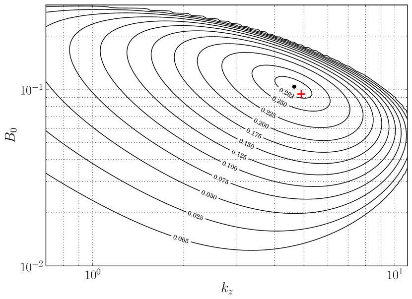
Figure 21: Stability map with the parameters from Kersalé et al. (2004). Our maximal growth rate is marked with a black dot, theirs is marked with a red cross.

Since we look for axisymmetric configurations, we can reduce the number of variables and naturally ensure the $\nabla\cdot B=0$ condition using the vector potential $A_{\varphi}$ such that $B_{r}=-\partial_{z}A_{\varphi}$ and $B_{z}=D_{r}A_{\varphi}$. The linearized induction equations become:

$$\begin{split}\partial_{t}B^{\prime}_{\varphi}&=B_{0}\partial_{z}v^{\prime}_{\varphi}+\sigma\partial_{z}^{2}B^{\prime}_{\varphi}\\ &+\ell_{\mathrm{H}}B_{0}\partial_{z}\left(\partial_{z}^{2}-\partial_{r}D_{r}-\partial_{r}\left[\Omega r\right]\right)\left[A^{\prime}_{\varphi}\right]\\ &+\eta\left(\partial_{r}^{2}+\frac{1}{r}\partial_{r}-\frac{1}{r^{2}}\right)\left[B^{\prime}_{\varphi}\right]\end{split}$$ (37)

$$\partial_{t}\left[-\partial_{z}A^{\prime}_{\varphi}\right]=B_{0}\partial_{z}v^{\prime}_{r}-\sigma\partial_{z}\left(\partial_{z}^{2}+\partial_{r}D_{r}\right)\left[A^{\prime}_{\varphi}\right]+\ell_{\mathrm{H}}B_{0}\partial_{z}B^{\prime}_{\varphi}$$ (38)

with $\sigma\equiv\eta+\gamma B_{0}^{2}$. At this stage, we have a linear system of partial differential equations for the the six fields $\bm{\xi}\equiv(\rho^{\prime},v^{\prime}_{r},v^{\prime}_{\varphi},v^{\prime}_{z},B^{\prime}_{\varphi},A^{\prime}_{\varphi})$, which we can write $\partial_{t}\,\bm{\xi}=\Delta\cdot\bm{\xi}$. Noticing that the periodic $z$ coordinate appears only in derivatives, we can replace it by a parameter $ik_{z}$ and reduce the problem to a system of one-dimensional equations. Expanding over a finite set of Chebyshev polynomials, the extraction of eigenmodes amounts to solving the generalized eigenvalue problem $\Delta\cdot\bm{\xi_{k}}=\omega_{k}\Gamma\!\cdot\bm{\xi_{k}}$, where $\Gamma$ is almost the identity matrix, in which a few lines are used to implement boundary conditions.

In order to test this method, we tried to reproduce the stability map from figure 3.a of Kersalé et al. (2004). The setup is the same as the one described in 3.2, including viscosity and ohmic resistivity with diffusivities $\nu=\eta=0.003$ and no Hall effect. The maximal growth rate is computed for different values of the background magnetic field $B_{0}$ and vertical wave number $k_{z}$ of the eigenmode. The spectral resolution used for this map is set to 32 modes after checking on several points that resolutions of 256, 64 or even 16 spectral modes gave the same eigenvalue to better than $10^{-4}$ relative accuracy.

The resulting map is shown in Fig. 21. Our unstable domain is geometrically very similar to the one of Kersalé et al. (2004), but extends on a larger portion of the $\left(k_{z},B_{0}\right)$ plane and displays larger growth rates. This comes from our different choice of boundary conditions for $v_{\varphi}$ and $B_{\varphi}$. Our maximal growth rate $\gamma_{M}\approx 0.266\Omega_{0}$ at $k_{z}=4.64r_{0}^{-1}$, $B_{0}=0.10$ is nevertheless very close to the one they found in this plane.

Appendix B Numerical setup of O’Keeffe & Downes (2014)

We present here the numerical setup of O’Keeffe & Downes (2014) and make the connection of their parameters real units to our dimensionless parameters.

O’Keeffe & Downes (2014) use a cubic box of size $L_{x}=L_{y}=2.6$ and $L_{z}=0.195$. The setup is a quarter disk with $r_{\mathrm{int}}=0.5$ and $r_{\mathrm{ext}}=2.58$. The units are so that 1 numerical length unit corresponds to $5.2\,\mathrm{a.u.}$ (O’Keefe 2013, p 80). This means, the disk extends from $r_{0}=2.6\,AU$ to $r_{1}=13.4\,AU$.

This cylindrical disk is filled with a flow of uniform initial density with $\rho=1.17\times 10^{-11}\,\mathrm{g.cm}^{-3}$ and a mean molecular mass $m_{\mathrm{n}}=\,m_{\mathrm{H}}$ which gives a number density $n=7\times 10^{12}\,\mathrm{cm}^{-3}$. The ionisation fraction is assumed to be $4\times 10^{-11}$ which implies a electron density of $n_{e}=2.82\times 10^{2}\,\mathrm{cm}^{-3}$.

The initial field strength is chosen to be $50\,\mathrm{mG}$, so that the Alfvén speed is

$$V_{\mathrm{A}}=\frac{B}{\sqrt{4\pi\rho}}=4.12\times 10^{3}\,\mathrm{cm.s}^{-1}.$$ (39)

The sound speed is not mentioned in O’Keeffe & Downes (2014) but may be found in O’Keefe (2013), p.81: $c_{s}=8.04\times 10^{4}\,\mathrm{cm.s}^{-1}$. This sound speed is coherent with a gas made of $\mathrm{H}_{2}$ at $T=130\,\mathrm{K}$.

With the values quoted above, we get the following dimensionless parameters

$$\frac{h}{r_{0}} =0.39,$$ (40)

$$\frac{c_{s}}{\Omega_{0}r_{0}} =4.35\times 10^{-2},$$ (41)

$$\frac{V_{\mathrm{A}}}{\Omega_{0}r_{0}} =2.23\times 10^{-3},$$ (42)

$$\frac{\ell_{H}}{r_{0}}\equiv\frac{c\sqrt{\rho\pi}}{2\pi en_{e}h} =5.5\times 10^{-3}.$$ (43)

The surprising low relative strength of the Hall effect ($\ell_{H}/h=1.4\times 10^{-2}\ll 1$) comes from the high ionisation fraction and the low midplane density compared to other models (e.g. Wardle 2007), and the large geometrical thickness compared to the pressure scale height ($h\Omega_{0}/c_{s}=9$)