Optical lattice influenced geometry of quasi-2D binary condensates and quasiparticle spectra

Abstract

We explore the collective excitations of optical lattices filled with two-species Bose-Einstein condensates (TBECs). We use a set of coupled discrete nonlinear Schrödinger equations to describe the system, and employ Hartree-Fock-Bogoliubov (HFB) theory with the Popov approximation to analyze the quasiparticle spectra at zero temperature. The ground state geometry, evolution of quasiparticle energies, structure of quasiparticle amplitudes, and dispersion relations are examined in detail. The trends observed are in stark contrast to the case of TBECs only with a harmonic confining potential. One key observation is the quasiparticle energies are softened as the system is tuned towards phase separation, but harden after phase separation and mode degeneracies are lifted.

I Introduction

The experimental realization of ultracold atoms in optical lattices has opened up a plethora of new possibilities to study interacting quantum many-body systems. The optical lattices, filled with bosons Greiner et al. (2001); Jaksch et al. (1998) or fermions Köhl et al. (2005); Hofstetter et al. (2002) provide unprecedented precision, tunability of interactions, possibility to generate different geometries and mimic the external gauge fields to study many-body systems Dalibard et al. (2011). These are near ideal systems to observe quantum phenomena such as superfluidity Anderson and Kasevich (1998); Fisher et al. (1989), quantum phase transition Greiner et al. (2002); Altman et al. (2005), Bloch oscillations Ben Dahan et al. (1996); Berg-Sørensen and Mølmer (1998), Landau-Zener tunneling Wu and Niu (2000); Liu et al. (2002), and various kind of instabilities Konotop and Salerno (2002); Chen and Wu (2010). In fact, the energy of collective excitations has emerged as fundamental and versatile tool to investigate many-body physics. An example of synergy between theory and experiment in this field is the study of the effect of tunneling and mean-field interaction of trapped 2D optical lattices on the collective excitation. Theoretically, Krämer et al. Krämer et al. (2002) studied it in detail, and Fort et al. Fort et al. (2003) verified the theoretical findings in experiments. A detailed understanding of the excitations of superfluid phase in optical lattices is possible with controlled variation of the lattice potential, and are excellent proxies to probe the properties of more complex condensed-matter counterparts. In this work, we examine the quasiparticle spectrum of condensates with tight binding approximation, and the condensate density is described through a set of coupled discrete nonlinear Schrödinger equations.

The introduction of a second species in the optical lattices, two-species BECs (TBECs) in lattices, creates a versatile model to probe diverse phenomena in physics. These are promising candidates to explain phenomena associated with fermionic correlations Paredes and Cirac (2003), phase separation Alon et al. (2006), hydrodynamical instability Lundh and Martikainen (2012) and novel phases Duan et al. (2003); Kuklov and Svistunov (2003). One remarkable property of TBECs is the phase segregation, which occurs when the interspecies interaction is stronger than the geometric mean of the intraspecies interactions Ho and Shenoy (1996). To date, TBECs in optical lattices have been experimentally realized in two different atomic species Catani et al. (2008) and two different hyperfine states of the same atomic species Gadway et al. (2010); Soltan-Panahi et al. (2011). It must be emphasized that TBECs with harmonic potential only have been realized in two different species of alkali-atoms Modugno et al. (2002); Lercher et al. (2011); McCarron et al. (2011); Thalhammer et al. (2008), and in two different isotopes Papp et al. (2008), and in two different hyperfine states Myatt et al. (1997); Stamper-Kurn et al. (1998); Hall et al. (1998); Tojo et al. (2010). These experiments have examined phase separation and other phenomena which are unique to binary BECs. The phenomenon of phase separation and transition from miscible-to-immiscible or vice versa has also been the subject of several theoretical studies Esry et al. (1997); Öhberg and Stenholm (1998); Svidzinsky and Chui (2003); Roy et al. (2014). These recent developments are motivations to probe the rich physics associated with TBECs in optical lattices. In recent works, we have investigated the fluctuation induced instability of dark solitons in TBECs Roy and Angom (2014) and change in the topology of the TBECs in quasi-1D lattices Suthar et al. (2015). However, to study the effects of fluctuations, either quantum or thermal, in optical lattices filled with TBECs it is essential to have a comprehensive understanding of the quasiparticle spectra.

In this paper, we examine the evolution of the quasiparticle spectra of TBECs in quasi-2D optical lattices at zero temperature. For this we use HFB formalism with Popov approximation, and tune one of the inter-atomic interactions to drive the TBEC from miscible to immiscible phase. In the immiscible domain, we show that the ground state has side-by-side density profile. This is in contrast to the case of quasi-1D system, where the ground state has sandwich density profile. To identify the geometry of the ground state, we examine the quasiparticle spectra using Bogoliubov de Gennes (BdG) analysis. For a stable ground state configuration, the spectra is real, but complex for metastable states. Following BdG analysis, we further examine the dispersion relation of binary system in optical lattices. These relations are used to understand the structure of the lower and higher energy excitations for miscible and immiscible domain of TBEC in lattice system. The dispersion relations are important to understand the nature of the excitations Stamper-Kurn et al. (1999); Steinhauer et al. (2002); Ticknor (2014), and Bragg spectroscopy Du et al. (2010) of ultracold quantum gases. These spectroscopic studies present full momentum-resolved measurements of the band structure and the associated interaction effects at several lattice depths Ernst et al. (2010). In fact, these relations have proved the presence of the rotonlike excitation in trapped dipolar BECs Wilson et al. (2010); Ticknor et al. (2011); Bisset and Blakie (2013); Blakie et al. (2013).

The paper is organized as follows: In Sec. II, we describe the HFB-Popov formalism and the dispersion relations for TBEC confined in optical lattices. The quasiparticle mode evolution and characteristic of the quasiparticle excitations with dispersion curves are presented in Sec. III. Finally, we conclude with the key finding of the present work in the Sec. IV.

II Theory and methods

Consider TBEC of dilute atomic gases in an optical lattice with a harmonic oscillator potential as a confining envelope potential. So, the net external potential is

$$V^{k}(\mathbf{r}) = V^{k}_{\rm ho}+V^{k}_{\rm latt}$$ (1)

$$= \frac{m_{k}}{2}(\omega_{x}^{2}x^{2}+\omega_{y}^{2}y^{2}+\omega_{z}^{2}z^{2})+V_{0}[\sin^{2}(2\pi x/\lambda_{L})$$

$$+\sin^{2}(2\pi y/\lambda_{L})+\sin^{2}(2\pi z/\lambda_{L})],$$

where $k=1,2$ denotes the species index, $m_{k}$ is the atomic mass of the $k$th species, $\omega_{i}(i=x,y,z)$ are the frequencies of the harmonic potential along each direction, $V_{0}=sE_{R}$ is the depth of the lattice potential in terms of the recoil energy $E_{R}=\hbar^{2}k^{2}_{L}/2m$ and dimensionless scale factor $s$. Here, $k_{L}=2\pi/\lambda_{L}$ is the wave number of the laser beam with wavelength $\lambda_{L}$ used to generate the optical lattice, and hence the lattice constant of the system is $a=\lambda_{L}/2$. It is to be noted that we consider the same external potential for both the condensate, and at $T=0$ K the grand canonical Hamiltonian of the system is

$$\hat{H} = \sum_{k=1}^{2}\int d\mathbf{r}~{}\hat{\Psi}^{\dagger}_{k}(\mathbf{r})\bigg{[}-\frac{\hbar^{2}{\nabla}^{2}}{2m_{k}}+V^{k}(\mathbf{r})-\mu_{k}+\frac{U_{kk}}{2}\hat{\Psi}^{\dagger}_{k}(\mathbf{r})$$

$$\times \hat{\Psi}_{k}(\mathbf{r})\bigg{]}\hat{\Psi}_{k}(\mathbf{r})+U_{12}\int d\mathbf{r}~{}\hat{\Psi}^{\dagger}_{1}(\mathbf{r})\hat{\Psi}^{\dagger}_{2}(\mathbf{r})\hat{\Psi}_{1}(\mathbf{r})\hat{\Psi}_{2}(\mathbf{r}),$$

where $\hat{\Psi}_{k}$, $\mu_{k}$ and $U_{kk}$ are the bosonic field operator, chemical potential and intraspecies interaction strength of $k$th species, and $U_{12}$ is the interspecies interaction strength. In the present study, we consider all the interactions to be repulsive, that is $U_{kk},U_{12}>0$. If the lattice is deep, i.e. $V_{0}\gg\mu_{k}$, the tight binding approximation (TBA) is applicable, and bosons occupy only the lowest energy band. In this approximation, the condensate is well localized within each lattice site, and the field operator for each of the species can be written as

$$\hat{\Psi}_{k}(\mathbf{r})=\sum_{\xi}\hat{a}_{k\xi}\phi_{k\xi}(\mathbf{r}),$$ (3)

where $\hat{a}_{k\xi}$ is the annihilation operator of the $k$th species at the lattice site with identification index $\xi$, which is a unique combination of the lattice index along $x$, $y$ and $z$ axes. The basic element of TBA lies in the definition of $\phi_{k\xi}(\mathbf{r})$, these are orthonormalized on-site Gaussian wave functions localized at the $\xi$th lattice site. Using the above definition of $\hat{\Psi}_{k}(\mathbf{r})$ in Eq. (LABEL:grand_can), we get the Bose-Hubbard Hamiltonian (BH) of the system.

II.1 HFB-Popov approximation for quasi-2D TBEC in optical lattices

To create a potential suitable to generate quasi-2D TBEC in optical lattices, set the frequencies to satisfy the condition $\omega_{x}=\omega_{y}=\omega_{\perp}\ll\omega_{z}$. The excitations along the tight or high frequency, $z$-axis, are of higher energies and we consider the condensate is in ground state along the $z$-axis at low temperatures $T\ll\hbar\omega_{z}/k_{B}$ with $k_{B}$ as the Boltzmann constant. Hence, the excitations of importance for quantum and thermal fluctuations are along the radial direction. In the TBA, the BH Hamiltonian which describes the system is

$$\hat{H}= \sum_{k=1}^{2}\left[-J_{k}\sum_{\langle\xi\xi^{\prime}\rangle}\hat{a}^{\dagger}_{k\xi}\hat{a}_{k\xi^{\prime}}+\sum_{\xi}(\epsilon^{(k)}_{\xi}-\mu_{k})\hat{a}^{\dagger}_{k\xi}\hat{a}_{k\xi}\right]$$ (4)

$$+ \frac{1}{2}\sum_{k=1}^{2}U_{kk}\sum_{\xi}\hat{a}^{\dagger}_{k\xi}\hat{a}^{\dagger}_{k\xi}\hat{a}_{k\xi}\hat{a}_{k\xi}$$

$$+ U_{12}\sum_{\xi}\hat{a}^{\dagger}_{1\xi}\hat{a}_{1\xi}\hat{a}^{\dagger}_{2\xi}\hat{a}_{2\xi},$$

where the index $\xi$ covers all the lattice sites. The summation index $\langle\xi\xi^{\prime}\rangle$ represents the nearest-neighbour, for illustration take $\xi\equiv(i,j)$ with $i$ and $j$ as labels of a lattice site along $x$ and $y$ axes, respectively. The possible values of $\xi^{\prime}$ in $\langle\xi\xi^{\prime}\rangle$ are then $(i-1,j)$, $(i+1,j)$, $(i,j-1)$, and $(i,j+1)$. The operator $\hat{a}_{k\xi}(\hat{a}^{\dagger}_{k\xi})$ is the bosonic annihilation (creation) operator of the $k$th species at the $\xi$th lattice site, and $J_{k}$s are the tunneling matrix elements. The effect of the envelope harmonic trapping potentials is subsumed in the offset energy $\epsilon^{(k)}_{\xi}=\Omega(i^{2}+j^{2})$. Here, $\Omega=m\omega^{2}_{\perp}a^{2}/2$ is the strength of the harmonic confinement. For simplicity, we assume the tunneling strength of the two species are identical in both $x$ and $y$ axes. For large tunneling strength and density, $J_{k}\gg\nu U_{kk},\nu U_{12}$ with $\nu$ as the filling factor, the bosons remain in superfluid phase. In this regime, the equilibrium properties of the system at $T=0$ K is well described by the 2D coupled discrete nonlinear Schrödinger equations (DNLSEs)

$$\mu_{1}c_{\xi}= - J_{1}\sum_{\xi^{\prime}}c_{\xi^{\prime}}+\left[\epsilon^{(1)}_{\xi}+U_{11}n^{c}_{1\xi}+U_{12}n^{c}_{2\xi}\right]c_{\xi},$$

(5a)

$$\mu_{2}d_{\xi}= - J_{2}\sum_{\xi^{\prime}}d_{\xi^{\prime}}+\left[\epsilon^{(2)}_{\xi}+U_{22}n^{c}_{2\xi}+U_{12}n^{c}_{1\xi}\right]d_{\xi},$$

where $c_{\xi}\equiv c_{i,j}$ and $d_{\xi}\equiv d_{i,j}$ are the complex amplitudes associated with the condensate wave functions of each species, and satisfy the normalization conditions $\sum_{\xi}|c_{\xi}|^{2}=\sum_{\xi}|d_{\xi}|^{2}=1$. The summation $\xi^{\prime}$ is over the nearest neighbours to the site $\xi$, more explicitly

$$\sum_{\xi^{\prime}}c_{\xi^{\prime}}\equiv c_{\xi-1}+c_{\xi+1}\equiv c_{i-1,j}+c_{i+1,j}+c_{i,j-1}+c_{i,j+1}.$$ (6)

From the definition of $\phi_{k\xi}$, in Eq.(5) $n^{c}_{1\xi}=|c_{\xi}|^{2}$ and $n^{c}_{2\xi}=|d_{\xi}|^{2}$ are the condensate densities of the first and second species at the $\xi$th lattice site, respectively. In the Bogoliubov approximation, we define the annihilation operators as $\hat{a}_{1\xi}=(c_{\xi}+\hat{\varphi}_{1\xi})e^{-i\mu_{1}t/\hbar}$, $\hat{a}_{2\xi}=(d_{\xi}+\hat{\varphi}_{2\xi})e^{-i\mu_{2}t/\hbar}$, and the new definition of the creation operators are the hermitian conjugates. The operator parts, ($\hat{\varphi}_{1\xi}$ or $\hat{\varphi}_{2\xi})$ represent small perturbations, and identify with the quantum and thermal fluctuations in the system. This approximation, when used in Eq. (4), partition the BH Hamiltonian to terms of different orders in the fluctuation operators. The lowest (zeroth) order term leads to the time-independent DNLSEs [Eq. (5)]. The leading order correction terms, linear in $\hat{\varphi}$, describe the effects arising from quantum and thermal fluctuations of the system. A more detailed description of the derivation is given in one of our previous works Suthar et al. (2015). The normal modes of the fluctuations, or the quasiparticle operators are defined through the Bogoliubov transformation

$$\hat{\varphi}_{k\xi} = \sum_{l}\left[u^{l}_{k\xi}\hat{\alpha}_{l}e^{-i\omega_{l}t}-v^{*l}_{k\xi}\hat{\alpha}^{\dagger}_{l}e^{i\omega_{l}t}\right],$$ (7a)

$$\hat{\varphi}^{\dagger}_{k\xi} = \sum_{l}\left[u^{*l}_{k\xi}\hat{\alpha}^{\dagger}_{l}e^{i\omega_{l}t}-v^{l}_{k\xi}\hat{\alpha}_{l}e^{-i\omega_{l}t}\right],$$ (7b)

where $u^{l}_{k\xi}$ and $v^{l}_{k\xi}$ are the quasiparticle amplitudes for the $k$th species in quasi-2D optical lattice potential, and $\omega_{l}=E_{l}/\hbar$ is the frequency of the $l$th quasiparticle mode with $E_{l}$ as the mode excitation energy. Further more, the quasiparticle amplitudes satisfy the normalization condition

$$\sum_{k\xi}\left(u^{*l}_{k\xi}u^{l^{\prime}}_{k\xi}-v^{*l}_{k\xi}v^{l^{\prime}}_{k\xi}\right)=\delta_{ll^{\prime}}.$$ (8)

Here $\hat{\alpha}_{l}(\hat{\alpha}^{\dagger}_{l})$ are the quasiparticle annihilation (creation) operators, which satisfy the Bose commutation relations. The above transformation diagonalizes the BH Hamiltonian, and taking into account the terms of higher order in fluctuation operators in total Hamiltonian leads to the HFB-Popov equations

$$E_{l}u^{l}_{1,\xi}= - J_{1}(u^{l}_{1,\xi-1}+u^{l}_{1,\xi+1})+\mathcal{U}_{1}u^{l}_{1,\xi}-U_{11}c^{2}_{\xi}v^{l}_{1,\xi}$$ (9a)

$$+ U_{12}c_{\xi}(d^{*}_{\xi}u^{l}_{2,\xi}-d_{\xi}v^{l}_{2,\xi}),$$

$$E_{l}v^{l}_{1,\xi}= J_{1}(v^{l}_{1,\xi-1}+v^{l}_{1,\xi+1})+\underline{\mathcal{U}}_{1}v^{l}_{1,\xi}+U_{11}c^{*2}_{\xi}u^{l}_{1,\xi}$$ (9b)

$$- U_{12}c^{*}_{\xi}(d_{\xi}v^{l}_{2,\xi}-d^{*}_{\xi}u^{l}_{2,\xi}),$$

$$E_{l}u^{l}_{2,\xi}= - J_{2}(u^{l}_{2,\xi-1}+u^{l}_{2,\xi+1})+\mathcal{U}_{2}u^{l}_{2,\xi}-U_{22}d^{2}_{\xi}v^{l}_{2,\xi}$$ (9c)

$$+ U_{12}d_{\xi}(c^{*}_{\xi}u^{l}_{1,\xi}-c_{\xi}v^{l}_{1,\xi}),$$

$$E_{l}v^{l}_{2,\xi}= J_{2}(v^{l}_{2,\xi-1}+v^{l}_{2,\xi+1})+\underline{\mathcal{U}}_{2}v^{l}_{2,\xi}+U_{22}d^{*2}_{\xi}u^{l}_{2,\xi}$$ (9d)

$$- U_{12}d^{*}_{\xi}(c_{\xi}v^{l}_{1,\xi}-c^{*}_{\xi}u^{l}_{1,\xi}),$$

where $\mathcal{U}_{1}=2U_{11}(n^{c}_{1\xi}+\tilde{n}_{1\xi})+U_{12}(n^{c}_{2\xi}+\tilde{n}_{2\xi})+(\epsilon^{(1)}_{\xi}-\mu_{1})$, $\mathcal{U}_{2}=2U_{22}(n^{c}_{2\xi}+\tilde{n}_{2\xi})+U_{12}(n^{c}_{1\xi}+\tilde{n}_{1\xi})+(\epsilon^{(2)}_{\xi}-\mu_{2})$ with $\underline{\mathcal{U}}_{k}=-\mathcal{U}_{k}$. The density of the noncondensate atoms at the $\xi$th lattice site is

$$\tilde{n}_{k\xi}=\sum_{l}[(|u^{l}_{k\xi}|^{2}+|v^{l}_{k\xi}|^{2})N_{0}(E_{l})+|v^{l}_{k\xi}|^{2}],$$ (10)

with $N_{0}(E_{l})$ as the Bose-factor of the system with energy $E_{l}$ at temperature $T$. The last term in the $\tilde{n}_{k\xi}$ is quantum fluctuations which is independent of the Bose-factor, and hence represents the quantum fluctuations of the system.

II.2 Dispersion relations of binary BEC

The dispersion relations, in general, determines how a system responds to external perturbations. So, in TBECs in optical lattices as well, it is important to examine the dispersion relations to understand how the system evolves after applying an external perturbation. Examples of current interest are topological defects generated through phase imprinting, evacuating single or multiple lattice sites, and tuning the lattice or harmonic potential parameters. To study the dispersion relation of the quasiparticles in optical lattices with a background trapping potential, we follow the definition in Ref. Wilson et al. (2010). Following which, we take the Fourier transform of the quasiparticle amplitudes, and compute the expectation value of the linear momentum $\langle k_{\xi}\rangle$ of each quasiparticle. So, in the momentum-space representation, for the $l$th quasiparticle

$${\langle k_{\xi}\rangle}_{l}=\left[\frac{\sum_{\alpha}\int d{{\bf k_{\xi}}}k^{2}_{\xi}[\tilde{u}^{l}_{\alpha}({\bf k_{\xi}})+\tilde{v}^{l}_{\alpha}({\bf k_{\xi}})]}{\sum_{\alpha}\int d{{\bf k_{\xi}}}[\tilde{u}^{l}_{\alpha}({\bf k_{\xi}})+\tilde{v}^{l}_{\alpha}({\bf k_{\xi}})]}\right]^{1/2},$$ (11)

where $k_{\xi}=(k_{i},k_{j})$ is the lattice site dependent wave-number and $\alpha=1,2$ is the index for species. Here $\tilde{u}^{l}_{\alpha}({\bf k_{\xi}})=\mathcal{F}[{u}^{l}_{\alpha}(\xi)]$, and $\tilde{v}^{l}_{\alpha}({\bf k_{\xi}})=\mathcal{F}[{v}^{l}_{\alpha}(\xi)]$ are the lattice site dependent quasiparticle amplitudes in momentum space, with $\mathcal{F}$ representing the Fourier transform. We, then, determine the discrete form of the dispersion relation by associating $\langle k_{\xi}\rangle_{l}$ to the excitation energies $E_{l}$. For TBECs in harmonic potential the dispersion curves were examined in a previous work, and reported unique trends in the miscible and immiscible regimes Ticknor (2014). Compared to which the presence of the optical lattice potential is expected to modify the dispersive properties of the systems in the present study. To examine the differences, and identify unique trends we compute $\langle k_{\xi}\rangle_{l}$ and study the dispersion curves in miscible and immiscible domains.

II.3 Numerical methods

To solve the coupled DNLSEs in Eq. (5) at $T=0$ K, we first scale the equations and rewrite in dimensionless form Suthar et al. (2015). The equations are then solved using the fourth order Runge-Kutta method. For the zero temperature computations we begin by neglecting the noncondensate density ($\tilde{n}_{k\xi}$) at each lattice site, and choose the initial guess values of the complex amplitudes with Gaussian or side-by-side envelope profile such that the quasiparticle energy spectrum is real. To obtain ground state of the system, we solve the DNLSEs with imaginary-time propagation. As described earlier, in the TBA, we take a basis set consisting of orthonormalized Gaussian functions localized at each lattice site. Hence, the basis set size or the number of basis functions is equal to the number of lattice sites in the system. Furthermore, to obtain the excitation spectrum we cast HFB-Popov Eqs. (9) as a matrix eigenvalue equation. For the computations at $T=0$ K, the matrix is diagonalized using the routine ZGEEV, routine to diagonalize non-symmetric matrix with complex elements, from the LAPACK library Anderson et al. (1999) to obtain the quasiparticle energies and amplitudes $E_{l}$, and $u^{l}_{\xi}$’s and $v^{l}_{\xi}$’s, respectively. However, when $T\neq 0$ K a larger number of basis functions is required to obtain a correct description of the thermal fluctuations, and this increases the dimension of the matrix corresponding to Eqs. (9). It is then better to use ARPACK Lehoucq et al. (1998) library for diagonalization as it is faster, and provides the option to compute a limited set of eigenvalues and eigen functions. The other advantage of using ARPACK is the optimal storage of large sparse matrices. In the latter part of our work to compute the dispersion curves, which in the present approach require quasiparticle amplitudes in the momentum representation, we use the FFTW library Frigo and Johnson (2005) in Intel MKL.

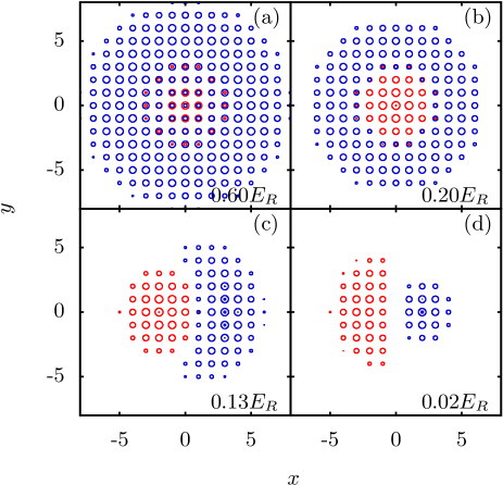
Figure 1: The geometry of the condensate density profiles and its transition from miscible to the immiscible domain for ⁸⁷Rb -⁸⁵Rb TBEC. (a) At higher $U_{22}$, the density of both species partially overlap, (b) as we decrease $U_{22}$ it changes into sandwich-type profile. At a critical value of $U_{22}$ ($0.16E_{R}$), both condensate segregate and rotational symmetry is broken, which results in side-by-side density profile in immiscible domain shown in (c,d). Here species labeled $1(2)$ is shown as red (blue) contours.

III Results and discussions

To examine the mode evolution of quasi-2D TBEC in optical lattices, we consider two cases from the experimentally realized TBECs, ⁸⁷Rb - ⁸⁵Rb Papp et al. (2008) and ¹³³Cs - ⁸⁷Rb  McCarron et al. (2011); Lercher et al. (2011). The former and latter are examples of TBECs with negligible, and large mass differences between the species, respectively. Another basic difference is, starting from miscible phase, the passage to the immiscible phase. In the ⁸⁷Rb - ⁸⁵Rb TBEC, the background scattering length of ⁸⁵Rb is negative, and hence to obtain stable ⁸⁵Rb condensate Cornish et al. (2000) it is essential to render it repulsive using magnetic Feshbach resonance Courteille et al. (1998); Roberts et al. (1998). The same can be employed to drive the system from miscible to immiscible domain. On the other hand, in ¹³³Cs - ⁸⁷Rb TBEC, the inter-species scattering length is tuned through a magnetic Feshbach resonance Pilch et al. (2009) to steer the TBEC from miscible to immiscible domain or vice-versa.

For the ⁸⁷Rb - ⁸⁵Rb TBEC, we assume ⁸⁷Rb and ⁸⁵Rb as the first and second species, respectively. For simplicity, and ease of comparison without affecting the results, the radial trapping frequency of the two species are chosen to be identical $\omega_{x}=\omega_{y}=2\pi\times 50$ Hz, with $\omega_{\perp}/\omega_{x}=20.33$. The wavelength of the laser beam to create the 2D lattice potential and lattice depth are $\lambda_{L}=1064$ nm and $V_{0}=5E_{R}$, respectively. To improve convergence, and have a good description of the optical lattice properties, we take the total number of atoms $N_{1}=N_{2}=300$ confined in a ($30\times 30$) lattice system. We use these set of parameters to study the ¹³³Cs - ⁸⁷Rb TBEC as well.

III.1 Mode evolution of trapped TBEC at $T=0$ K

To solve the DNLSE we consider Gaussian basis function of width $0.3a$, where $a$ is the lattice constant, to evaluate the lattice parameters. In the case of ⁸⁷Rb - ⁸⁵Rb TBEC, the tunneling matrix elements are $J_{1}=0.66E_{R}$ and $J_{2}=0.71E_{R}$, and $U_{11}$ = $0.07E_{R}$ and $U_{12}$ = $0.15E_{R}$ are the intraspecies and interspecies interactions, respectively. The difference in the values of $J_{1}$ and $J_{2}$ arises from the mass difference of the species in the TBEC system. Following the same steps, the parameters for the ¹³³Cs - ⁸⁷Rb TBEC are $J_{1}=0.66E_{R}$, $J_{2}=1.70E_{R}$, $U_{11}$ = $0.96E_{R}$ and $U_{22}$ = $0.42E_{R}$. In both the cases, we drive the system from miscible to immiscible phase, and examine the evolution of the modes in detail.

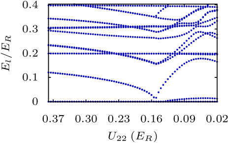
Figure 2: The evolution of the low-lying quasiparticle modes as a function of the intraspecies interaction ($U_{22}$) for the ⁸⁷Rb-⁸⁵Rb TBEC held in quasi-2D optical lattices. Here $U_{22}$ is in units of the recoil energy $E_{R}$.

III.1.1 ⁸⁷Rb - ⁸⁵Rb TBEC

As mentioned earlier $U_{22}$, the intraspecies interaction of ⁸⁵Rb, is decreased to drive the TBEC from miscible to immiscible domain. The changes in the ground state density profile are shown in Fig. 1. In the miscible domain, the profiles overlap and there is a shift in the position of the density maxima as $U_{22}$ is decreased [Fig. 1(b)]. At a critical value $U_{22}^{\rm c}$, the two species undergo phase separation with side-by-side density profiles and breaks the rotational symmetry. The features of the quasiparticles too change in tandem with the density profile, and the variation of the excitation energies with $U_{22}$ are shown in Fig. 2.

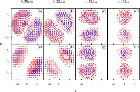
Figure 3: The evolution of quasiparticle amplitude corresponding to the slosh mode of first species (a-d) and second species (e-h) in ⁸⁷Rb -⁸⁵Rb TBEC as $U_{22}$ is decreased from $0.30E_{R}$ to $0.05E_{R}$. The value of $U_{22}$ is shown at the top of the figures. Here the red contours represent the quasiparticle amplitude ($u_{1}(x,y)$ and $u_{2}(x,y)$), whereas the blue contours represent the quasihole amplitude ($v_{1}(x,y)$ and $v_{2}(x,y)$). The density perturbation is from dotted contours to the solid contours.

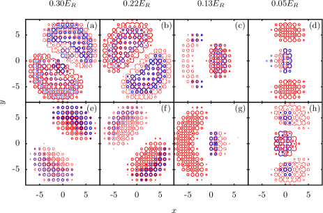
Figure 4: The evolution of the quasiparticle amplitude corresponding to the other slosh mode, which is degenerate to the mode shown in Fig. 3 in miscible domain. These amplitudes correspond to the first species (a-d) and second species (e-h) of ⁸⁷Rb -⁸⁵Rb TBEC with the change in $U_{22}$, which is shown at the top of the figures. At a critical value of $U_{22}$, this mode hardens and gets transformed into an interface mode (d, h). Here the red contours represent the quasiparticle amplitude, whereas the blue contours represent the quasihole amplitude.

To obtain the mode evolution curves, we do a series of computations starting from the miscible domain of the system (higher $U_{22}$), and decrease $U_{22}$ to values below $U_{22}^{\rm c}$.

In the miscible domain, all the excitation modes are doubly degenerate. As $U_{22}$ is lowered, eigen energies of modes with different phases of $u_{1}$ and $u_{2}$, or out-of-phase modes decrease in energy, and degeneracy is lifted when $U_{22}$ is below $U_{22}^{\rm c}$. The slosh and Kohn modes are the two lowest energy ones in the miscible domain, and are associated with the out-of-phase and in-phase modes, respectively. The structure of the two degenerate slosh modes are shown in Fig. 3(a,b,e,f) and Fig. 4(a,b,e,f). In general, the doubly degenerate modes are $\pi/2m$ rotation of each other, where $m$ is the azimuthal quantum number. For the slosh modes this property is evident from the figures. One of the degenerate slosh modes goes soft at $U_{22}^{\rm c}=0.16$, in particular, it is the one which is in-phase with the condensate density, but the other slosh mode gains energy at phase separation. Thus, below $U_{22}^{\rm c}$ the degeneracy of the slosh modes is lifted. On further decrease of $U_{22}$ one striking effect of the optical lattice potential is observed: the soft slosh mode gains energy and is transformed into an interface mode. This is in stark contrast to the case without the lattice potential, where the mode remains soft Ticknor (2013). This is also apparent from the nature of the quasiparticle amplitudes shown in the figures. The Kohn mode, on the other hand, remains steady with an energy of $0.2E_{R}$.

Considering the general trend, there are only mode crossings in the miscible domain, however, both mode crossing and avoided crossings occur in the phase-separated domain. Prior to phase separation, out-of-phase modes decrease in energy as $U_{22}$ is lowered, but the in-phase modes remain steady. So, no mode mixing occurs when modes of the former type encounters the latter, and they cross each other. However, when $U_{22}$ is below the critical value, degeneracies are lifted, and mode mixing can occur. This explains the presence of avoided crossings in the phase-separated domain. The energies of the out-of-phase modes decrease monotonically with decrease in $U_{22}$ as it favours phase separation. After phase separation, these modes get hardened due to rotational symmetry breaking. It must be noted that, as shown in Fig.  1(b), the density profiles are shell structured or rotationally symmetric for intermediate values of $U_{22}$. However, there is a sharp transition to side-by-side density profile as phase-separation occurs when $U_{22}$ is lowered.

III.1.2 ¹³³Cs - ⁸⁷Rb TBEC

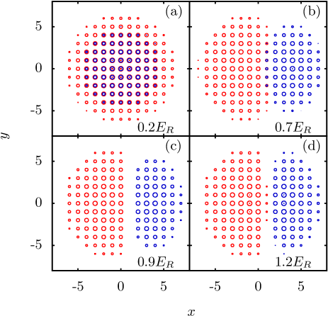
Figure 5: The geometry of the condensate density profiles and its transition from miscible to the immiscible domain in ¹³³Cs -⁸⁷Rb TBEC. Here species labeled $1(2)$ is shown as red (blue) contours.

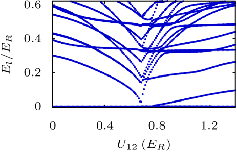
Figure 6: The evolution of the low-lying modes as a function of the interspecies interaction in ¹³³Cs-⁸⁷Rb TBEC held in quasi-2D optical lattices. Here $U_{12}$ is in units of the recoil energy $E_{R}$.

For the ¹³³Cs - ⁸⁷Rb TBEC, as mentioned earlier, we vary interspecies interaction $U_{12}$ to induce the miscible to the immiscible phase transition.

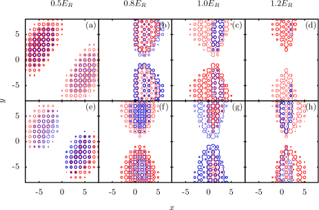
Figure 7: The evolution of quasiparticle amplitude corresponding to the slosh mode of first species (a-d) and second species (e-h) of ¹³³Cs -⁸⁷Rb TBEC as $U_{12}$ is increased from $0.5E_{R}$ to $1.2E_{R}$. The value of $U_{12}$ is shown at the top of the figures. Here the red contours represent the quasiparticle amplitude ($u_{1}(x,y)$ and $u_{2}(x,y)$), whereas the blue contours represent the quasihole amplitude ($v_{1}(x,y)$ and $v_{2}(x,y)$).

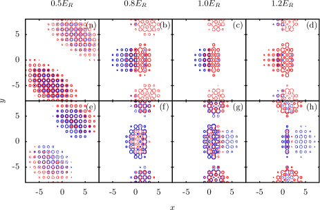
Figure 8: The evolution of the quasiparticle mode corresponding to the slosh mode, which is degenerate with the mode shown in Fig. 7 in miscible domain. These amplitudes correspond to the first species (a-d) and second species (e-h) of ¹³³Cs -⁸⁷Rb TBEC as $U_{12}$ is increased from $0.5E_{R}$ to $1.2E_{R}$. The value of $U_{12}$ is shown at the top of the figures. At a critical value of $U_{12}$, the energy of the mode increases and it gets transformed into an interface mode. Here the red contours represent the quasiparticle amplitude, whereas the blue contours represent the quasihole amplitude.

The density profiles, as the miscible-to-immiscible transition occurs, are shown in Fig. 5. The change, except for the curvature at the interface, are similar to the case of ⁸⁷Rb - ⁸⁵Rb TBEC shown in Fig. 1. The evolution of the mode energies before, during and after the transition are shown in Fig. 6. Like in the previous case, ⁸⁷Rb - ⁸⁵Rb TBEC, the slosh mode is degenerate in the miscible domain [shown in Fig. 7(a,e) and Fig. 8(a,e)]. It goes soft at the critical value $U^{c}_{12}=0.68E_{R}$, and the degeneracy is lifted. As shown in Fig. 7(b,c,d,f,g,h) and Fig. 8(b,c,d,f,g,h), the evolution of the non-degenerate modes are qualitatively similar to that of ⁸⁷Rb - ⁸⁵Rb TBEC. One key feature in the general trend of the mode evolution is, in the miscible domain all the mode energies decrease with increase in $U_{12}$. However, as discussed earlier, in ⁸⁷Rb - ⁸⁵Rb TBEC the energies of all the in-phase modes (modes with same phase of $u_{1}$ and $u_{2}$) remain steady. At phase separation, the mode energies reach minimal values and then, increase with increasing $U_{12}$ in the immiscible domain. To gain an insight on these trends, we examine the dependence on various parameters with a series of computations.

Based on the results, we observe that the form of the interaction, interspecies or intraspecies, which is tuned to drive the miscible-to-immiscible transition has an impact on the trends of the mode evolution. An important observation is, for high $U_{kk}/J_{k}$ all the modes decrease in energy, in the miscible domain, when the interspecies interaction is tuned. However, when the intraspecies interaction is tuned all the in-phase modes remain steady. Thus, we attribute the difference in the trends to the geometry of the interface at phase separation. When the interspecies interaction is tuned, as in ¹³³Cs - ⁸⁷Rb TBEC, the interface at phase separation is linear as evident from Fig. 5(c). Thus, it can align with the nodes of the mode functions, and decrease all the mode energies. This is not possible in the other case, tuning intraspecies interaction in ⁸⁷Rb - ⁸⁵Rb, as the interface is curved as shown in Fig. 1(c).

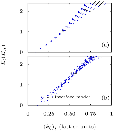
Figure 9: The discrete BdG quasiparticle dispersion curve in (a) miscible and (b) immiscible domain of ⁸⁷Rb -⁸⁵Rb TBEC.

III.2 Dispersion relations

To obtain dispersion curves, based on Eq. (11), we compute $\langle k_{\xi}\rangle_{l}$ of the $l$th quasiparticle, and plot the mode energies. To highlight trends in the dispersion curves dependent on angular momentum, we choose parameters different from what we have considered so far. Further more, we restrict ourselves to the case of ⁸⁷Rb - ⁸⁵Rb TBEC, where the trends in dispersion curves are more prominent due to weaker inter-atomic interactions, and small mass difference. In particular, we consider a system of ⁸⁷Rb - ⁸⁵Rb TBEC with DNLSE parameters $J_{1}=J_{2}=0.66E_{R}$, and $U_{11}=U_{22}=0.01E_{R}$. For the interspecies on-site interactions $U_{12}$, to explore the dispersion relations in miscible and immiscible domains we set it to $0.003E_{R}$ and $0.08E_{R}$, respectively. All the other parameters are retained with the same values as mentioned earlier. One important point to be emphasized is, unlike the parameters in the mode evolutions studies, the current choice of DNLSE parameters correspond to two different sets of $N_{1}$ and $N_{2}$.

III.2.1 Miscible domain

The ground state of the system has rotational symmetry in this domain. Hence, the azimuthal quantum number ($m$) is a good quantum number, and finite interspecies interaction mixes modes with same $m$ arising from each of the two species. This is reflected in the branch like structures in the dispersion curve as shown in Fig. 9(a). To understand the physics behind the structure of the dispersion curves, we examine the structure of the quasiparticle modes. For this, let us focus on modes which lie on three branches, marked by arrows, in Fig. 9(a). Each of the modes can be identified based on the value of $m$. As example, three of the low-energy ($\approx 1E_{R}$) and another three from higher energies ($\approx 2E_{R}$) are shown in Fig. 10.

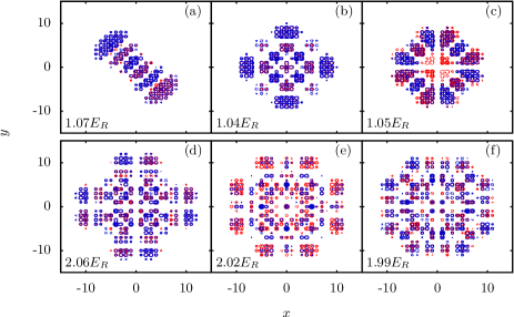
Figure 10: Shown here are the quasiparticle amplitudes in the miscible domain of a TBEC. (a-c) quasiparticle amplitudes with excitation energy ($\approx 1E_{R}$) and (d-f) quasiparticle amplitudes with excitation energy ($\approx 2E_{R}$). These quasiparticles are indicated in dispersion plot [Fig. 9(a)] by black circles. The excitation energies corresponding to each quasiparticle is written in the lower left corner of each plot in units of the recoil energy. Here excitations corresponding to species 1 (2) are shown with red (blue) contours.

The energies of the first three quasiparticle modes in the figure, Fig. 10(a-c), are out-of-phase type, and the values of $m$ are 1, 4 and 6. Among these modes, the first two modes have $\langle k_{\xi}\rangle_{l}\approx 0.42$, and are phonon-like as these lie on the linear part of the dispersion curve. However, the mode in Fig.  10(c) with $\langle k_{\xi}\rangle_{l}\approx 0.44$ and $m=6$ is a surface mode, which is evident from the structure of the mode function. The same observation is confirmed from the exponential decay in the numerical values of $u$ towards the center. These three modes show that within the same energy range ($\approx 1E_{R}$), phononlike and surface excitation co-exists. One discernible trend is, the modes with higher $m$ and $\langle k_{\xi}\rangle_{l}$ have extremas located farther from the center of the trap, and turn into surface modes. The quasiparticle amplitudes with higher excitation energies ($\approx 2E_{R}$), shown in Fig. 10(d,e,f), have intricate structures. This is as expected arising from the larger mode mixing due to higher density of states and non-zero $U_{12}$.

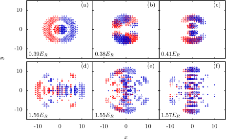
Figure 11: Shown here are the quasiparticle amplitudes in the immiscible domain of a TBEC. (a-c) quasiparticle amplitudes with excitation energy ($\approx 0.4E_{R}$) and (d-f) quasiparticle amplitudes with excitation energy ($\approx 1.5E_{R}$). These quasiparticles are indicated in dispersion plot [Fig. 9(b)] by black circles. The excitation energies corresponding to each quasiparticle is written in the lower left corner of each plot in units of the recoil energy. Here excitations corresponding to species 1 (2) are shown with red (blue) contours.

III.2.2 Immiscible domain

For the immiscible domain, the dispersion curve is as shown in Fig. 9(b), and there are no discernible trends. The reason is, in this domain the condensate density profile does not have rotational symmetry, and hence, there are mixing between quasiparticle modes with different $m$-values. To examine the structure of the mode functions we consider three each with energies $\approx 0.4E_{R}$ and $\approx 1.55E_{R}$, these are shown in Fig. 11(a-c), and Fig. 11(d-f), respectively. Consider the modes with energies $0.39E_{R}$ and $0.38E_{R}$ as shown in Fig. 11(a), and (b), the flow patterns in these are equivalent to the breathing and slosh modes in single species condensates, respectively. There is, however, one important difference: the density flow involves both the species, and have different velocity fields. The mode with energy $0.41E_{R}$, shown in Fig. 11(c), is out-of-phase in nature and has a different configuration compared to the two previous ones. That is, the mode functions are prominent around the interface region, and are negligible in the region where the condensate densities are maximal. In continuum case, modes with similar structure (interface mode) has been reported in recent works  Ticknor (2013, 2014). The mode with higher energies have enhanced mode mixing due to higher density of states, which is evident from the structure of the modes with $\approx 1.55E_{R}$ shown in Fig. 11(d-f). Hence, it is non-trivial to classify the modes like in the case of modes with energies $\approx 0.4E_{R}$. In terms of the geometrical structures, the modes in Fig. 11(d), (e), and (f) have extrema coincident with the condensates, interlaced distribution, and localized in the interface region, respectively. Thus, within a range of excitation energies, there exists modes with diverse characters.

IV Conclusions

Our studies show that the introduction of an optical lattice potential modifies the geometry of condensate density distribution of TBECs at phase separation. The sandwich or shell structured density profiles are no longer energetically favourable, and the side-by-side geometry emerges as the only stable ground state density profile. This arises from the higher interface energy due to the local density enhancements at lattice sites. The other important observation is, as the TBEC is tuned from miscible to immiscible phase, the evolution of the quasiparticle spectra can be grouped into two. The first group have quasiparticles which exhibit a decrease in the mode energies as we approach phase-separation, and reach minimal values at the critical interaction strength. However, the mode energies increase after crossing into the domain of phase-separation. The second group, on the other hand, remains steady as the interaction strength is tuned across the critical value. Furthermore, we have examined the dispersion curves for miscible and immiscible domains of TBEC. The curves, in the miscible domain, show discernible trends associated with the azimuthal quantum number of the quasiparticle. However, in the immiscible domain, there are no discernible trends associated with azimuthal quantum number. This is due to the rotational symmetry breaking of the condensate density profiles, and the resulting mixing of modes with different azimuthal quantum numbers.