Analytical study on parameter regions of dynamical instability for two-component Bose–Einstein condensates with coaxial quantized vortices

Abstract

The dynamical instability of weakly interacting two-component Bose–Einstein condensates with coaxial quantized vortices is analytically investigated in a two-dimensional isotopic harmonic potential. We examine whether complex eigenvalues appear on the Bogoliubov–de Gennes equation, implying dynamical instability. Rather than solving the Bogoliubov–de Gennes equation numerically, we rely on a perturbative expansion with respect to the coupling constant which enables a simple, analytic approach. For each pair of winding numbers and for each magnetic quantum number, the ranges of inter-component coupling constant where the system is dynamically unstable are exhaustively obtained. Co-rotating and counter-rotating systems show distinctive behaviors. The latter is much more complicated than the former with respect to dynamical instability, particularly because radial excitations contribute to complex eigenvalues in counter-rotating systems.

I INTRODUCTION

Dynamical instability is one of the most interesting phenomena in Bose–Einstein condensates of cold atomic gases. This instability is observed experimentally in various situations whose typical examples include the splitting of a multiply quantized vortex Shin and the decaying of a condensate flowing in an optical lattice Fallani . Theoretically, the dynamics of condensates are well described by the time-dependent Gross–Pitaevskii (TDGP) equation Dalfovo , and theoretical studies solving the TDGP equation successfully explained the experiment of vortex splitting Huhtamaki ; Munoz . When judging whether the condensate is dynamically unstable, we may employ the Bogoliubov–de Gennes (BdG) equation Bogoliubov ; deGennes ; Fetter , which is obtained by linearizing the TDGP equation. The BdG equation is a non-hermetian eigenvalue problem, giving complex eigenvalues as well as real eigenvalues, and we interpret the presence of complex eigenvalues as an indication of dynamical instability. By solving the BdG equation under given physical conditions, we can find regions of parameters in which the system is dynamically unstable.

The dynamical instability of a multiply quantized vortex in a single component system has been widely investigated. In this study, we consider multi-component systems with quantized vortices because understanding the instabilities in these systems is a difficult problem. Previous works on this matter numerically solve the differential equations (see Refs. Skryabin ; Ishino ; Wen ). The inter-component interaction and mutual influence between multiple vortices make the dynamical behavior of this system diverse and nontrivial. Therefore, it is not practical to solve the BdG equation numerically in the entire parameter space or to find all parameter regions of the dynamical instability. Such an exhaustive numerical study of the BdG equation on dynamically unstable regions is not easy even for a single component system with a multiply quantized vortex because some regions may be too small to be identified Kawaguchi .

The general properties of the BdG equation are well investigated Skryabin ; Kawaguchi ; Mine . To address its non-hermiticity, an inner product must be introduced with an indefinite metric, which guarantees orthonormality to the eigenfunction set. Then, eigenfunctions belonging to real eigenvalues are classified according to the sign of its squared norm into positive- and negative-norm eigenfunctions. On the other hand, the squared norm of an eigenfunction with a complex (non-real) eigenvalue is always zero. The degeneracy between positive- and negative-norm eigenfunctions, a kind of resonance, has been shown both numerically and analytically to be necessary for the emergence of complex eigenvalues Lundh ; Taylor ; Skryabin ; Kawaguchi . In our previous study Nakamura1 , we proposed a systematic method based on perturbation theory to find parameter regions in which complex eigenvalues emerge, namely regions where the system is dynamically unstable, starting from regions without complex eigenvalues. Because this method is simple in essence, it can be extended to multi-component systems.

The aim of this paper is to investigate the dynamical instability of two-component systems with two quantized vortices whose cores overlap according to the method in Ref. Nakamura1 . Determining whether such systems are unstable by solving the TDGP and BdG equations demands a heavy load of numerical calculations. In our method, we analytically solve algebraic equations, which are much simpler than the differential equations, and we can cover a wide area of parameters to exhaustively determine regions of dynamical instability without overlooking small regions. The only restrictions of our current study are that the coupling constants of the respective self-interactions and the inter-component interaction are assumed to be so small that the perturbative approach with respect to these coupling constants is allowed.

In Sect. II, a general formulation of the TDGP and BdG equations is reviewed for the two-dimensional, two-component condensate system trapped by a harmonic potential. We also review our analytic method based on the perturbation method in Ref. Nakamura1 , originally for a single component system, and consider its extension to a multi-component system in Sect. III. There, we emphasize that the degeneracy between the unperturbed positive- and negative-norm eigenstates is a necessary prerequisite to the emergence of complex eigenvalues. Section IV is the main part of this paper in which the formulations in the preceding sections are applied to a trapped two-component system with two coaxial quantized vortices. The unperturbed states are those with the vanishing intra- and inter-component coupling constants. A summary is given in Sect. V.

II GENERAL FORMULATION OF GROSS–PITAEVSKII AND BOGOLIUBOV–DE GENNES EQUATIONS FOR TWO COMPONENT CONDENSATE SYSTEM

We consider two-component condensates in the $x$-$y$ plane at zero temperature, trapped by a two-dimensional isotropic harmonic potential with trap frequency $\omega$. This condensate system can be realized as the limit of pancake-shaped condensates in a three-dimensional cylindrical harmonic potential with a very large trap frequency along the $z$-axis. The system is characterized by the order parameters, denoted by $\psi_{j}(\bm{x},t)$ ($j=1,2$ and ${\bm{x}}=(x,y)$), which satisfy the coupled TDGP equations,

$$i{\frac{\partial}{\partial t}}\psi_{j}(\bm{x},t)=\Bigl{\{}h_{0}-\mu_{j}$$

$$\quad+gN\beta_{jj}|\psi_{j}(\bm{x},t)|^{2}+gN\beta_{j\overline{j}}\left|\psi_{\overline{j}}(\bm{x},t)\right|^{2}\Bigr{\}}\psi_{j}(\bm{x},t)\,.$$ (1)

Here, we use the notation of $h_{0}=-\nabla^{2}/2m+m\omega^{2}(x^{2}+y^{2})/2$ and $\overline{j}=2,1$ for $j=1,2$ , and $\mu_{j}$ stands for the chemical potential of each component $j$ . Throughout this paper, $\hbar$ is set to unity. For simplicity, the masses and the condensate populations of the two species are taken to be the same and are denoted by $m$ and $N$, respectively. All interactions are assumed to be represented by two-body contact-type potentials, and the three independent coupling constants are $g\beta_{11}$ , $g\beta_{22}$ , and $g\beta_{12}=g\beta_{21}$ . The order parameters are normalized as

$$\int\!dxdy\,\left|\psi_{j}(\bm{x},t)\right|^{2}=1\,.$$ (2)

For the stationary Gross–Pitaevskii equations, the solutions are represented by $\xi_{j}(\bm{x})$,

$$\left(h_{0}-\mu_{j}+gN\beta_{jj}|\xi_{j}(\bm{x})|^{2}+gN\beta_{12}|\xi_{\overline{j}}(\bm{x})|^{2}\right)\xi_{j}(\bm{x})=0\,.$$ (3)

We suppose time evolution of the order parameters that slightly deviate from $\xi(\bm{x})$, i.e., $\psi_{j}(\bm{x},t)=\xi_{j}(\bm{x})+\delta\psi_{j}(\bm{x},t)$ . Substituting these parameters into Eq. (1) and linearizing the TDGP equations with respect to $\delta\psi_{j}$, we obtain

$$i\frac{\partial}{\partial t}\delta\psi_{j}(\bm{x},t)=\Bigl{\{}h_{0}-\mu_{j}$$

$$\qquad+2gN\beta_{jj}|\xi_{j}|^{2}+gN\beta_{12}|\xi_{\overline{j}}|^{2}\Bigr{\}}\delta\psi_{j}(\bm{x},t)$$

$$\qquad+gN\beta_{jj}\xi_{j}^{2}\delta\psi^{\ast}_{j}(\bm{x},t)+gN\beta_{12}\xi^{\ast}_{\overline{j}}\xi_{j}\delta\psi_{\overline{j}}(\bm{x},t)$$

$$\qquad+gN\beta_{12}\xi_{\overline{j}}\xi_{j}\delta\psi^{\ast}_{\overline{j}}(\bm{x},t)\,.$$ (4)

Then, $\delta\psi_{j}$ are expanded as

$$\delta\psi_{j}(\bm{x},t)=\sum_{q}\left\{u_{qj}(\bm{x})e^{-iE_{q}t}+v_{qj}^{\ast}(\bm{x})e^{iE_{q}^{\ast}t}\right\}\,.$$ (5)

Here, $u_{qj}$ and $v_{qj}$ are eigenfunctions of the following BdG equation,

$$\mathcal{T}\bm{u}_{q}=E_{q}\bm{u}_{q}\,,$$ (6)

where the quartet representation is introduced,

$$\bm{u}_{q} =\begin{pmatrix}u_{q1}\\ u_{q2}\\ v_{q1}\\ v_{q2}\end{pmatrix}\,,\qquad\qquad\mathcal{T}=\begin{pmatrix}\cal{L}&\cal{M}\\ -\cal{M}^{\ast}&-\cal{L}^{\ast}\end{pmatrix}\,,$$ (7)

$$\mathcal{L} =\begin{pmatrix}\mathcal{L}_{11}&\mathcal{L}_{12}\\ \mathcal{L}_{21}&\mathcal{L}_{22}\\ \end{pmatrix}\,,\qquad\cal{M}=\begin{pmatrix}\mathcal{M}_{11}&\mathcal{M}_{12}\\ \mathcal{M}_{21}&\mathcal{M}_{22}\end{pmatrix}\,,$$ (8)

$$\mathcal{L}_{jj} =h_{0}-\mu_{j}+2gN\beta_{jj}|\xi_{j}|^{2}+gN\beta_{12}|\xi_{\overline{j}}|^{2}\,,$$ (9)

$$\mathcal{M}_{jj} =gN\beta_{jj}\xi_{j}^{2}\,,$$ (10)

$$\mathcal{L}_{12} =\mathcal{L}_{21}^{\ast}=gN\beta_{12}\xi_{2}^{\ast}\xi_{1}\,,$$ (11)

$$\mathcal{M}_{12} =\mathcal{M}_{21}=gN\beta_{12}\xi_{2}\xi_{1}\,.$$ (12)

We define the indefinite inner product for any pair of quartets ${\bm{s}}(\bm{x})$ and ${\bm{t}}(\bm{x})$ by

$$(\bm{s},\bm{t})=\int\!dxdy\,\bm{s}^{\dagger}(\bm{x})\tau_{3}{\bm{t}}(\bm{x})\,,\quad\tau_{i}=\sigma_{i}\otimes 1=\begin{pmatrix}I&0\\ 0&-I\end{pmatrix}\,,$$ (13)

where $\sigma_{i}$ ($i=1,2,3$ ) are the Pauli matrices, operating on the space of the doublet $(u_{j},v_{j})$, and $I$ is a $2\times 2$ unit matrix with respect to the index $j$ . The symmetric property,

$$\tau_{3}\mathcal{T}\tau_{3}=\mathcal{T}^{\dagger}\,,$$ (14)

leads to the pseudo-Hermiticity of $\mathcal{T}$,

$$(\bm{s},\mathcal{T}\bm{t})=(\mathcal{T}\bm{s},\bm{t})\,.$$ (15)

The squared norm of ${\bm{s}}(\bm{x})$,

$$\|\bm{s}\|^{2}=(\bm{s},\bm{s})\,,$$ (16)

can be positive, negative, and zero. Because the unperturbed eigenfunctions relevant to our discussion belong solely to real eigenvalues, we do not repeat the properties of eigenfunctions belonging to complex and zero eigenvalues. The symmetric property,

$$\tau_{1}\mathcal{T}\tau_{1}=-\mathcal{T}^{\ast}\,,$$ (17)

implies that, for each eigenfunction ${\bm{y}}_{q}$ ($\mathcal{T}{\bm{y}}_{q}=E_{q}{\bm{y}}_{q}$) belonging to a real eigenvalue that is normalized as $\|\bm{y}_{q}\|^{2}=1$, there is an eigenfunction ${\bm{z}}_{\tilde{q}}=\tau_{1}{\bm{y}}^{\ast}_{q}$ such that $\mathcal{T}\bm{z}_{\tilde{q}}=-E_{q}\bm{z}_{\tilde{q}}$ with $\|\bm{z}_{\tilde{q}}\|^{2}=-1$ . Note that $\bm{z}_{\tilde{q}}$ may be denoted simply by $\bm{z}_{q}$, but we adopt the notation $\bm{z}_{\tilde{q}}$ to make our expressions simpler. The explicit form of ${\tilde{q}}$ will be given below Eq. (40) in Sect. IV. The set of $\{\bm{y}_{q}\,,\,\bm{z}_{q}\}$ is orthonormal,

$$(\bm{y}_{q},\bm{y}_{q^{\prime}})=-(\bm{z}_{q},\bm{z}_{q^{\prime}})=\delta_{qq^{\prime}}\,,\qquad(\bm{y}_{q},\bm{z}_{q^{\prime}})=0\,,$$ (18)

and complete,

$$\sum_{q}\left[\bm{y}_{q}(\bm{x})\bm{y}^{\dagger}_{q}(\bm{x}^{\prime})-\bm{z}_{q}(\bm{x})\bm{z}^{\dagger}_{q}(\bm{x}^{\prime})\right]=\tau_{3}\delta(\bm{x}-\bm{x}^{\prime})\,.$$ (19)

III GENERAL ANALYTIC FORMULATION BASED ON PERTURBATION THEORY

The complex eigenvalue in the BdG equations (6) indicates the dynamical instability of the system. In this study, we seek the parameter regions of the emergence of complex eigenmodes following the analytical method in Ref. Nakamura1 , which was originally applied to a single component system. We extend the work of Ref. Nakamura1 to a two-component system as follows. We suppose the vicinity of a boundary in the parameter space and divide it into regions with and without complex eigenvalues. We solve the stationary GP eq. (3) and BdG eq. (6) to obtain their eigenvalues and eigenfunctions at a point belonging to the region without complex eigenvalues. These eigenvalues and eigenfunctions are regarded as unperturbative eigenvalues and eigenfunctions. We then consider small variations in the parameters and develop a perturbative expansion to find complex eigenvalues in the first order of the expansion when the parameter variation crosses the boundary.

We develop the perturbative expansion as follows. First, the quantities in the GP equation are expanded as

$$\xi_{j}(\bm{x}) = \xi_{j}^{(0)}(\bm{x})+\varepsilon\xi_{j}^{(1)}(\bm{x})+O(\varepsilon^{2})\,,$$ (20)

$$\mu_{j} = \mu_{j}^{(0)}+\varepsilon\mu_{j}^{(1)}+O(\varepsilon^{2})\,,$$ (21)

where $\varepsilon$ is an infinitesimal parameter that characterizes the parameter variation. The expansion of the matrix $\mathcal{T}$, which involves both $\xi_{j}$ and $\mu_{j}$, is

$$\mathcal{T}=\mathcal{T}_{0}+\varepsilon\mathcal{T}^{\prime}+O(\varepsilon^{2})\,,$$ (22)

where

$$\mathcal{L}=\mathcal{L}_{0}+\varepsilon\mathcal{L}^{\prime}+O(\varepsilon^{2})\,,\quad\mathcal{M}=\mathcal{M}_{0}+\varepsilon\mathcal{M}^{\prime}+O(\varepsilon^{2})\,,$$ (23)

and

$$\mathcal{T}_{0}=\begin{pmatrix}\mathcal{L}_{0}&\mathcal{M}_{0}\\ -\mathcal{M}_{0}^{\ast}&-\mathcal{L}_{0}^{\ast}\\ \end{pmatrix}\,,\qquad\mathcal{T}^{\prime}=\begin{pmatrix}\mathcal{L}^{\prime}&\mathcal{M}^{\prime}\\ -\mathcal{M}^{\prime\ast}&-\mathcal{L}^{\prime\ast}\\ \end{pmatrix}\,.$$ (24)

Note that the symmetric properties (14) and (17) are respected in the perturbative expansion and that the properties of the indefinite inner product are preserved at any order of the perturbation.

Likewise, the eigenfunctions and eigenvalues of the BdG equations are expanded as $\bm{u}_{q}^{(0)}+\varepsilon\bm{u}_{q}^{(1)}+O(\varepsilon^{2})$ and $E_{q}=E_{q}^{(0)}+\varepsilon E_{q}^{(1)}+O(\varepsilon^{2})\,$, respectively. The zeroth-order equations are

$$\mathcal{T}_{0}\bm{u}_{q}^{(0)}=E_{q}^{(0)}\bm{u}_{q}^{(0)}\,,$$ (25)

and the first-order equations are organized as

$$(\mathcal{T}_{0}-E_{q}^{(0)})\bm{u}_{q}^{(1)}=(E_{q}^{(1)}-\mathcal{T}^{\prime})\bm{u}_{q}^{(0)}\,.$$ (26)

Assuming that $E_{q}^{(0)}$ is real, we examine whether $E_{q}^{(1)}$ is complex. According to Ref. Nakamura1 , the necessary prerequisite to complex $E_{q}^{(1)}$ is a degeneracy between $\bm{y}^{(0)}_{q}$ and $\bm{z}^{(0)}_{q}$  but not between $\bm{y}^{(0)}_{q}$’s nor $\bm{z}^{(0)}_{q}$’s. For a single $E_{q}^{(0)}$, consider a general situation in which there are $r$-fold degenerate $\bm{y}^{(0)}_{qi}$ $(i=1,2,\cdots,r)$ and $s$-fold degenerate $\bm{z}^{(0)}_{q^{\prime}i^{\prime}}$ $(i^{\prime}=1,2,\cdots,s)$ , i.e., a total of $r+s$ degenerate states. Here, $\bm{z}^{(0)}_{q^{\prime}}$ is the solution of

$$\mathcal{T}_{0}\bm{z}_{q^{\prime}}^{(0)}\left(=-E_{\tilde{q}^{\prime}}^{(0)}\bm{z}_{q^{\prime}}^{(0)}\right)=E_{q}^{(0)}\bm{z}_{q^{\prime}}^{(0)}\,.$$ (27)

Then, $\bm{u}_{q}^{(0)}$ is generally given by their linear combination,

$$\bm{u}_{q}^{(0)}=\sum_{i=1}^{r}c_{yi}\bm{y}_{qi}^{(0)}+\sum_{i^{\prime}=1}^{s}c_{zi^{\prime}}\bm{z}_{q^{\prime}i^{\prime}}^{(0)}\,.$$ (28)

Substituting this linear expression into Eq. (26), we obtain the secular equation for $E_{q}^{(1)}$ ,

$$\begin{vmatrix}\left(\bm{y}_{q1}^{(0)},\mathcal{T}^{\prime}\bm{y}_{q1}^{(0)}\right)-E_{q}^{(1)}&\cdots&\left(\bm{y}_{q1}^{(0)},\mathcal{T}^{\prime}\bm{z}_{{q^{\prime}}1}^{(0)}\right)&\cdots\\ \vdots&\ddots&\vdots&\ddots\\ \left(\bm{z}_{{q^{\prime}}1}^{(0)},\mathcal{T}^{\prime}\bm{y}_{q1}^{(0)}\right)&\cdots&\left(\bm{z}_{{q^{\prime}}1}^{(0)},\mathcal{T}^{\prime}\bm{z}_{{q^{\prime}}1}^{(0)}\right)+E_{q}^{(1)}&\cdots\\ \vdots&\ddots&\vdots&\ddots\end{vmatrix}$$

$$=0\,.$$ (29)

Multiplying each row from the $(r+1)$-th row to the $(r+s)$-th row by $-1$, we rewrite this secular equation as

$$\left|T^{\prime}-E_{q}^{(1)}\right|=0\,,$$ (30)

with

$$T^{\prime} =\begin{pmatrix}L_{y}&M\\ -M^{\dagger}&-L_{z}\end{pmatrix}\,,\quad (L_{y})_{ii^{\prime}} =\left(\bm{y}_{qi}^{(0)},\mathcal{T}^{\prime}\bm{y}_{qi^{\prime}}^{(0)}\right)$$ (31)

$$(L_{z})_{ii^{\prime}} =\left(\bm{z}_{{q^{\prime}}i}^{(0)},\mathcal{T}^{\prime}\bm{z}_{{q^{\prime}}i^{\prime}}^{(0)}\right)\,,\quad M_{ii^{\prime}} =\left(\bm{y}_{qi}^{(0)},\mathcal{T}^{\prime}\bm{z}_{{q^{\prime}}i^{\prime}}^{(0)}\right)\,.$$ (32)

It can be proven from the pseudo-Hermiticity of $\mathcal{T}^{\prime}$ that $L_{y}^{\dagger}=L_{y}$ and $L_{z}^{\dagger}=L_{z}$. When $M$ does not vanish, $T^{\prime}$ is non-Hermitian, and $E_{q}^{(1)}$ can be complex.

Our procedure for investigating the dynamical instability of a system consists of the following four steps. (1) We find appropriate zeroth-order BdG equations with real eigenvalues and solve the equations to obtain $\bm{y}^{(0)}$ and $\bm{z}^{(0)}$ . (2) The condition for the degeneracy between $\bm{y}^{(0)}$ and $\bm{z}^{(0)}$ is determined. (3) The secular equation involving degenerate $\bm{y}^{(0)}_{qi}$ and $\bm{z}^{(0)}_{{q^{\prime}}i^{\prime}}$ is established. (4) We verify whether the first-order eigenvalue $E^{(1)}_{q}$ is complex or real by solving the secular equation.

IV APPLICATION TO TWO-COMPONENT QUANTIZED VORTICES

In this study, we consider a trapped two-component system with quantized vortices, characterized by winding numbers $\kappa_{j}$ for component $j$  $(j=1,2)$ . Both vortex cores are located at the center of the trapping potential, which is set to the origin. We assume that all particle interactions, both intra- and inter-component interactions, are weak. That is, the coupling constant $g$ in Eq. (1) is a small parameter on the order of $\varepsilon$, and a perturbation expansion with respect to $g$ is developed. For this purpose, we replace $g$ with $\varepsilon g$ . Then, the vortex solutions of the stationary GP equations with $\kappa_{j}$ are

$$\xi_{j}(r,\theta)=\sqrt{\frac{1}{2\pi}}e^{i\kappa_{j}\theta}f_{j}(r)\,,$$ (33)

where $r$ and $\theta$ are the polar coordinates. Without loss of generality, the range of $\kappa_{j}$’s may be restricted to

$$\kappa_{1}\geq 0\,,\qquad\kappa_{1}\geq|\kappa_{2}|\,.$$ (34)

We call the rotations for $\kappa_{2}\geq 0$ and $\kappa_{2}<0$ co- and counter-rotations, respectively.

IV.1 Zeroth-Order BdG Equations

For $g=0$, the BdG equations (25) are linear Schrödinger equations under the isotropic harmonic potential and can be solved analytically, irrespective of the stationary solutions of the GP equations. All eigenvalues are real.

The zeroth-order eigenvalues and eigenfunctions of the BdG equations are labeled by $q=(n,\ell,j)$; $n\,,\,\ell$ being the principal and magnetic quantum numbers, respectively, and $j$ representing the component index. To give the eigenfunctions of the BdG and GP equations, we introduce the eigenfunctions $\phi_{n\ell j}$ ,

$$\left\{h_{0}-\mu^{(0)}_{j}\right\}\phi_{n\ell j}=E^{(0)}_{n\ell j}\phi_{n\ell j}\,,$$ (35)

which are given by

$$E^{(0)}_{n\ell j} =\omega\left(2n+|\ell+\kappa_{j}|+1\right)-\mu_{j}^{(0)}\,$$ (36)

$$n =0,1,2,\cdots\,,\qquad\ell=0,\pm 1,\pm 2\,,\cdots\,,$$ (37)

and

$$\phi_{n\ell j}(\rho,\theta)=\sqrt{\frac{1}{2\pi}}e^{i(\ell+\kappa_{j})\theta}R_{n\ell j}(\rho)\,,$$ (38)

with $\rho=\sqrt{m\omega}r$ . The explicit forms of $R_{n\ell j}(\rho)$ are presented in Appendix A. The zeroth-order BdG eigenfunctions are

$$\bm{y}_{n\ell 1}^{(0)} =\begin{pmatrix}\phi_{n\ell 1}\\ 0\\ 0\\ 0\end{pmatrix}\,,\qquad \bm{y}_{n\ell 2}^{(0)} =\begin{pmatrix}0\\ \phi_{n\ell 2}\\ 0\\ 0\end{pmatrix}\,,$$ (39)

$$\bm{z}_{n\ell 1}^{(0)} =\begin{pmatrix}0\\ 0\\ \phi_{n-\ell 1}^{\ast}\\ 0\end{pmatrix}\,,\qquad \bm{z}_{n\ell 2}^{(0)} =\begin{pmatrix}0\\ 0\\ 0\\ \phi_{n-\ell 2}^{\ast}\end{pmatrix}\,.$$ (40)

Note the definition $\tilde{q}=(n,-\ell,j)$ for $q=(n,\ell,j)$, which implies that $\bm{z}_{n\ell j}=\tau_{1}\bm{y}_{n-\ell j}^{*}$ and that the eigenvalues of $\bm{y}_{n\ell j}$ and $\bm{z}_{n\ell j}$ are $E^{(0)}_{n\ell j}$ and $E^{(0)}_{n-\ell j}$, respectively. We normalize $\phi_{n\ell j}$,

$$\int_{0}^{\infty}\int_{0}^{2\pi}\left|\phi_{n\ell j}(\rho,\theta)\right|^{2}\,rdrd\theta=1\,,$$ (41)

so

$$(\bm{y}_{n\ell j},\bm{y}_{n^{\prime}\ell^{\prime}j^{\prime}})=-(\bm{z}_{n\ell j},\bm{z}_{n^{\prime}\ell^{\prime}j^{\prime}})=\delta_{nn^{\prime}}\delta_{\ell\ell^{\prime}}\delta_{jj^{\prime}}\,.$$ (42)

IV.2 Zeroth- and First-Order GP Equations

The zeroth-order stationary GP equations are

$$h_{0}\xi_{j}^{(0)}=\mu_{j}^{(0)}\xi_{j}^{(0)}\,.$$ (43)

Their solutions, which are the lowest eigenstates, are found to be

$$\xi_{j}^{(0)}(\rho,\theta)=\phi_{00j}(\rho,\theta)\,,\qquad\mu_{j}^{(0)}=\omega\left(|\kappa_{j}|+1\right)\,.$$ (44)

Next, we have the first-order stationary GP equations,

$$\left\{h_{0}-\mu_{j}^{(0)}\right\}\xi^{(1)}_{j}$$

$$=-\left(gN\beta_{jj}\left|\xi^{(0)}_{j}\right|^{2}+gN\beta_{12}\left|\xi^{(0)}_{\overline{j}}\right|^{2}-\mu_{j}^{(1)}\right)\xi^{(0)}_{j}\,.$$ (45)

Multiplying both sides by $\xi_{j}^{(0)\ast}$ and integrating them over the whole two-dimensional space, we obtain the first-order chemical potentials $\mu_{j}^{(1)}$ as

$$\mu_{j}^{(1)}=m\omega F\left(\frac{\beta_{jj}}{2^{2|\kappa_{j}|}}\frac{(2|\kappa_{j}|)!}{(|\kappa_{j}|!)^{2}}+\frac{\beta_{12}}{2^{(\kappa_{1}+|\kappa_{2}|)}}\frac{(\kappa_{1}+|\kappa_{2}|)!}{\kappa_{1}!|\kappa_{2}|!}\right)\,,$$ (46)

with $F={gN}/{2\pi}\,.$

IV.3 First-Order Matrix Elements

The $\theta$-dependence of the first-order matrix $\mathcal{T}^{\prime}$ in Eq. (24) can be factorized as

$$\mathcal{T}^{\prime}=\begin{pmatrix}\mathcal{U}&0\\ 0&\mathcal{U}^{\dagger}\\ \end{pmatrix}\begin{pmatrix}\mathcal{L}^{\prime}_{r}&\mathcal{M}^{\prime}_{r}\\ -\mathcal{M}^{\prime}_{r}&-\mathcal{L}^{\prime}_{r}\\ \end{pmatrix}\begin{pmatrix}\mathcal{U}^{\dagger}&0\\ 0&\mathcal{U}\\ \end{pmatrix}\,,$$ (47)

where the $r$-dependent matrix is

$$\mathcal{L}^{\prime}_{r} =-\begin{pmatrix}\mu^{(1)}_{1}&0\\ 0&\mu^{(1)}_{2}\\ \end{pmatrix}+2F\begin{pmatrix}\beta_{11}R_{001}^{2}&0\\ 0&\beta_{22}R_{002}^{2}\\ \end{pmatrix}$$

$$\hskip 20.0pt+F\beta_{12}\begin{pmatrix}R_{002}^{2}&R_{001}R_{002}\\ R_{001}R_{002}&R_{001}^{2}\\ \end{pmatrix}\,,$$ (48)

$$\mathcal{M}^{\prime}_{r} =F\begin{pmatrix}\beta_{11}R_{001}^{2}&\beta_{12}R_{001}R_{002}\\ \beta_{12}R_{001}R_{002}&\beta_{22}R_{002}^{2}\\ \end{pmatrix}\,,$$ (49)

and the $\theta$-dependent unitary matrix $\mathcal{U}$ is

$$\mathcal{U}=\begin{pmatrix}e^{i\kappa_{1}\theta}&0\\ 0&e^{i\kappa_{2}\theta}\\ \end{pmatrix}\,.$$ (50)

It follows from Eq. (47) that all phase factors $e^{i\kappa_{j}\theta}$ in the integrands of the matrix elements (31)–(32) are canceled out and that only phase factors $e^{i\ell\theta}$ from $\bm{y}_{q,i}^{(0)}$ and $\bm{z}_{{q^{\prime}},i^{\prime}}^{(0)}$ survive. Therefore, after $\theta$-integration, the matrix elements carry $\delta_{\ell\ell^{\prime}}$. The matrix elements are evaluated as follows:

$$\phantom{=}\left(\bm{y}_{n\ell j}^{(0)},{\cal T}^{\prime}\bm{y}_{n^{\prime}\ell^{\prime}j}^{(0)}\right)=\left(\bm{z}_{n{-}\ell j}^{(0)},{\cal T}^{\prime}\bm{z}_{n^{\prime}{-}\ell^{\prime}j}^{(0)}\right)^{\ast}$$

$$=\delta_{\ell\ell^{\prime}}\left[-\delta_{nn^{\prime}}\mu_{j}^{(1)}\right.+2F\beta_{jj}\int\!rdr\left\{R_{00j}^{2}R_{n\ell j}R_{n^{\prime}\ell j}\right\}$$

$$\phantom{=\left(\bm{y}_{n\ell j}^{(0)},{\cal T}^{\prime}\bm{y}_{n^{\prime}\ell^{\prime}j}^{(0)}\right)}\left.+F\beta_{12}\int\!rdr\left\{R_{00\overline{j}}^{2}R_{n\ell j}R_{n^{\prime}\ell j}\right\}\right]\,,$$ (51)

$$\phantom{=}\left(\bm{y}_{n\ell j}^{(0)},{\cal T}^{\prime}\bm{y}_{n^{\prime}\ell^{\prime}\overline{j}}^{(0)}\right)=\left(\bm{z}_{n{-}\ell j}^{(0)},{\cal T}^{\prime}\bm{z}_{n^{\prime}{-}\ell^{\prime}\overline{j}}^{(0)}\right)^{\ast}$$

$$=\delta_{\ell\ell^{\prime}}F\beta_{12}\int\!rdr\left\{R_{00j}R_{00\overline{j}}R_{n\ell j}R_{n^{\prime}\ell\overline{j}}\right\}\,,$$ (52)

$$\phantom{=}\left(\bm{y}_{n\ell j}^{(0)},{\cal T}^{\prime}\bm{z}_{n^{\prime}{-}\ell^{\prime}j}^{(0)}\right)=\left(\bm{z}_{n^{\prime}{-}\ell^{\prime}j}^{(0)},{\cal T}^{\prime}{\bm{y}}_{n\ell j}^{(0)}\right)^{\ast}$$

$$=\delta_{\ell{-}\ell^{\prime}}F\beta_{jj}\int\!rdr\left\{R_{00j}^{2}R_{n\ell j}R_{n^{\prime}-\ell{j}}\right\}\,,$$ (53)

$$\phantom{=}\left(\bm{y}_{n\ell j}^{(0)},{\cal T}^{\prime}\bm{z}_{n^{\prime}{-}\ell^{\prime}\overline{j}}^{(0)}\right)=\left(\bm{z}_{n^{\prime}{-}\ell^{\prime}\overline{j}}^{(0)},{\cal T}^{\prime}{\bm{y}}_{n\ell j}^{(0)}\right)^{\ast}$$

$$=\delta_{\ell{-}\ell^{\prime}}F\beta_{12}\int\!rdr\left\{R_{00j}R_{00\overline{j}}R_{n\ell j}R_{n^{\prime}-\ell\overline{j}}\right\}\,.$$ (54)

The above properties of the matrix elements allow matrix $T^{\prime}$ in Eq. (31) to be shifted to a block diagonal form. We classify the degenerate states $\bm{y}_{q}$’s and $\bm{z}_{q^{\prime}}$’s into groups according to the value of $\ell$, that is, $m_{f}$ groups labeled by $\ell=\ell_{1},\cdots,\ell_{m_{f}}$ . Rearranging the matrix elements according to the above groups, we obtain the following block diagonal matrix $T^{\prime}$:

$$T^{\prime}=\begin{pmatrix}T^{\prime}_{\ell_{1}}&0&0&0\\ 0&T^{\prime}_{\ell_{2}}&0&0\\ 0&0&\ddots&0\\ 0&0&0&T^{\prime}_{\ell_{m_{f}}}\\ \end{pmatrix}\,.$$ (55)

IV.4 Patterns of Degeneracy

Based on the conclusions of the previous subsection, complex $E^{(1)}$ can only appear in block matrix $T^{\prime}_{\ell_{m}}$  that includes both $\bm{y}_{q}$ and $\bm{z}_{q^{\prime}}$. In addition, the matrix $M_{\ell_{m}}$ in $T_{\ell_{m}}$ must be non-vanishing. We, therefore, seek conditions for non-vanishing $M_{\ell}=\left(\bm{y}_{n\ell j}^{(0)},\mathcal{T}^{\prime}\bm{z}_{n^{\prime}\ell j^{\prime}}^{(0)}\right)$ . Hereafter, the superscript ⁽⁰⁾ for $\bm{y}$ and $\bm{z}$ is implicit for the sake of simplicity. The eigenvalues of $\bm{y}_{n\ell j}$ and $\bm{z}_{n^{\prime}\ell j^{\prime}}$ are

$$E_{n\ell j}^{(0)} =\omega\left(2n+|\ell+\kappa_{j}|-|\kappa_{j}|\right)$$ (56)

$$-E_{n^{\prime}-\ell j^{\prime}}^{(0)} =-\omega\left(2n^{\prime}+|-\ell+\kappa_{j^{\prime}}|-|\kappa_{j^{\prime}}|\right)$$ (57)

The degeneracy condition between $\bm{y}_{n\ell j}$ and $\bm{z}_{n^{\prime}\ell j^{\prime}}$, namely $E_{n\ell j}^{(0)}=-E_{n^{\prime}-\ell j^{\prime}}^{(0)}$  is

$$2(n+n^{\prime})+|\ell+\kappa_{j}|+|\ell-\kappa_{j^{\prime}}|-|\kappa_{j}|-|\kappa_{j^{\prime}}|=0\,.$$ (58)

When complex $E^{(1)}_{q}$ is found, it can be shown from Eq. (14) that $E^{(1)}_{\tilde{q}}$ is also complex. Therefore, without loss of generality, $\ell$ can be restricted to $\ell\geq 0$ when searching for the condition for complex eigenvalues. The degeneracy is possible only when $E_{n\ell j}^{(0)}\leq 0$ and/or $-E_{n^{\prime}-\ell j^{\prime}}^{(0)}\geq 0$, which restricts the allowed value of $\ell$ to $0\leq\ell\leq-2\kappa_{j}$ for $\kappa_{j}\leq 0$ and $0\leq\ell\leq 2\kappa_{j^{\prime}}$ for $\kappa_{j^{\prime}}\geq 0$ . Finally, with Eq. (34), we only have to consider the range $0\leq\ell\leq 2\kappa_{1}$ . The solutions of Eq. (58) are categorized into the following four types of ($j,j^{\prime}$) :

1. $(j,j^{\prime})=(1,1)$: $n=n^{\prime}=0$ when $0<\ell\leq\kappa_{1}$

2. $(j,j^{\prime})=(2,2)$: $n=n^{\prime}=0$ when $0<\ell\leq|\kappa_{2}|$

3. $(j,j^{\prime})=(1,2)$: $n=n^{\prime}=0$ when $0<\ell\leq\kappa_{2}$

4. $(j,j^{\prime})=(2,1)$:

   • $n=n^{\prime}=0$     when $0<\ell\leq\kappa_{1}$ and $0\leq\kappa_{2}$

   • $n+n^{\prime}=-\kappa_{2}$ when $0\leq-\kappa_{2}\leq\ell\leq\kappa_{1}$

   • $n+n^{\prime}=\ell$     when $0<\ell\leq-\kappa_{2}$

   • $n+n^{\prime}=-\ell+\kappa_{1}-\kappa_{2}$ when $\kappa_{1}\leq\ell\leq\kappa_{1}-\kappa_{2}$

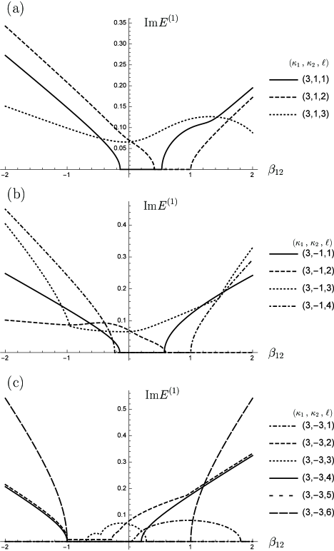
Figure 1: Regions with possible double degeneracy between $\bm{y}_{n\ell j}$ and $\bm{z}_{n^{\prime}\ell j^{\prime}}$ in the $\kappa_{2}-\ell$ plane for a fixed $\kappa_{1}>0$. They are (a) $\bm{y}_{0\ell 1}$ and $\bm{z}_{0\ell 1}$, (b) $\bm{y}_{0\ell 2}$ and $\bm{z}_{0\ell 2}$, (c) $\bm{y}_{0\ell 1}$ and $\bm{z}_{0\ell 2}$, (d) $\bm{y}_{n\ell 2}$ and $\bm{z}_{n^{\prime}\ell 1}$. The number inside each subregion denotes the value of $n+n^{\prime}$.

Note that the modes with $(n,\ell,j)=(0,0,1)\,,\,(0,0,2)$ are excluded from our considerations because they are zero modes. These modes remain as zero modes and never turn into complex modes under perturbation that retains the global phase symmetries $\xi_{j}\to\xi_{j}e^{i\delta_{j}}$ Takahashi2014 . From the inequality,

$$E_{0\ell j}^{(0)}+E_{0-\ell j^{\prime}}^{(0)}=|\ell+\kappa_{j}|+|\ell-\kappa_{j^{\prime}}|-|\kappa_{j}|-|\kappa_{j^{\prime}}|\geq 0$$ (59)

for $(j,j^{\prime})=(1,1),(2,2),(1,2)$ and $(j,j^{\prime})=(2,1)$ with $\kappa_{2}\geq 0$, we see that radial excited states $n+n^{\prime}\neq 0$ participate only in (d) with $\kappa_{2}<0$  implying counter-rotation.

The regions with double degeneracy in the $\kappa_{2}-\ell$ plane for a fixed $\kappa_{1}>0$ are depicted in Fig. 1. Collecting all these results, we obtain all possible multiply degenerate sets that contain both $\bm{y}$ and $\bm{z}$. They are categorized into the following five subregions: [A] $0<\ell\leq\kappa_{2}$,  [B] $0\leq\kappa_{2}<\ell\leq\kappa_{1}$,  [C] $0<-\kappa_{2}<\ell\leq\kappa_{1}$,  [D] $0<\ell\leq-\kappa_{2}$,  [E] $\kappa_{1}<\ell\leq\kappa_{1}-\kappa_{2}$  in Fig. 2. For example, in subregion C, where regions (a) and (d) with double degeneracy overlap one another but do not overlap regions (b) nor (c), we find two types of degenerate sets, namely ($\bm{y}_{0\ell 1}$,$\bm{y}_{-\kappa_{2}\ell 2}$,$\bm{z}_{0\ell 1}$) and ($\bm{y}_{n\ell 2}$,$\bm{z}_{n^{\prime}\ell 1}$), where $n+n^{\prime}=-\kappa_{2}$ and $n\neq-\kappa_{2}$. All types of degenerate sets are summarized in Table 1. The types are labeled by numbers representing degrees of degeneracy and by the additional indices $y,z,$ and $n$ in C, D and E.

Figure 2: Subregions with possible multiple degeneracies involving both $\bm{y}$ and $\bm{z}$. The boundaries denoted by solid lines or filled circles are included in the subregion while those denoted by dashed lines or open circles are excluded from the subregion.

For illustration, we count all degenerate sets for $\kappa_{1}=3$ in Fig. 3. Figure 3 and Table 1 provide general features of the appearance of the degenerate sets. In co-rotation, i.e., for $\kappa_{2}\geq 0$, there is only one degenerate set for each pair of $(\kappa_{2},\ell)$, which are either A₄ or B₃, and no radially excited state is involved. The degenerate patterns are richer in counter-rotations. The degenerate region extends to the maximum value $\ell=2\kappa_{1}$, which has been restricted to $\ell\leq\kappa_{1}$ for the co-rotating case. All degenerate sets involve radially excited states except for those on the line $\ell=-\kappa_{2}+\kappa_{1}$. There are plural degenerate sets for each $(\kappa_{2},\ell)$. In particular, there are $1-\kappa_{2}$ sets in subregion C, $1+\ell$ in D, and $1+\kappa_{1}-\kappa_{2}-\ell$ in E. These numbers increase around $\ell=\kappa_{1}$, where $-E_{0-\kappa_{1}1}$ is positive and reaches a maximum, and as $\kappa_{2}$ approaches $-\kappa_{1}$. The total number of degenerate sets for the winding number pair $(\kappa_{1},\kappa_{2})$, namely for that in each column in Table 1, is $\kappa_{1}-\kappa_{2}(\kappa_{1}+1)$ for the counter-rotating case and $\kappa_{1}$ for the co-rotating case including $\kappa_{2}=0$.

Table 1: All types of possible degeneracies involving both $\bm{y}$ and $\bm{z}$ in each subregion and the relevant eigenfunctions.

Subreg.	Symbol	Degenerate set of eigenfunctions
A	A4	($\bm{y}_{0\ell 1}$, $\bm{y}_{0\ell 2}$, $\bm{z}_{0\ell 1}$, $\bm{z}_{0\ell 2}$)
B	B3	($\bm{y}_{0\ell 1}$, $\bm{y}_{0\ell 2}$, $\bm{z}_{0\ell 1}$)
C	C3	($\bm{y}_{0\ell 1}$, $\bm{y}_{-\kappa_{2}\ell 2}$, $\bm{z}_{0\ell 1}$)
	C2n	($\bm{y}_{n\ell 2}$, $\bm{z}_{n^{\prime}\ell 1}$)  with $n+n^{\prime}=-\kappa_{2}$; $n\neq-\kappa_{2}$
D	D3y	($\bm{y}_{0\ell 1}$, $\bm{y}_{\ell\ell 2}$, $\bm{z}_{0\ell 1}$)
	D3z	($\bm{y}_{0\ell 2}$, $\bm{z}_{\ell\ell 1}$, $\bm{z}_{0\ell 2}$)
	D2n	($\bm{y}_{n\ell 2}$, $\bm{z}_{n^{\prime}\ell 1}$)  with $n+n^{\prime}=\ell$; $n,n^{\prime}\neq 0,\ell$
E	E2n	($\bm{y}_{n\ell 2}$, $\bm{z}_{n^{\prime}\ell 1}$)  with $n+n^{\prime}=\kappa_{1}-\kappa_{2}-\ell$

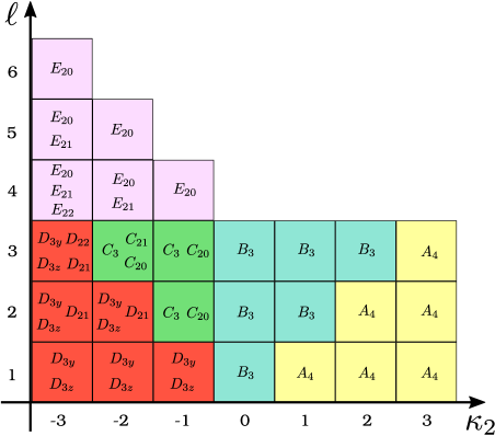
Figure 3: (Color online) All degenerate types for $\kappa_{1}=3$

IV.5 Range of Inter-Component Interaction Parameter $\beta_{12}$ of Complex Eigenvalues

First-order complex eigenvalues $E_{q}^{(1)}$ emerge only in subregions A–E, as shown above. Note that this is a prerequisite condition for the emergence of complex eigenvalues, and we have to verify the secular equation Eq. (30) to determine whether its solution is complex or real. We then study how the inter-component interaction affects the stability of a system with two vortices. Varying the inter-component interaction parameter $\beta_{12}$ with fixed $\beta_{11}=\beta_{22}=1$ for $\kappa_{1}=3$, we seek the ranges of $\beta_{12}$ in which some eigenvalues are complex. To this end, we manipulate only algebraic equations, which gives our study a clear advantage in numerical calculations over those that require solving the differential equations. Moreover, we use the discriminant $\Delta$ of the polynomial in the secure equation for doubly and triply degenerates sets and obtain the range of $\beta_{12}$ for $\Delta$. For quadruply degenerate sets $A_{4}$, we directly solve the secure equation and find the ranges of the complex eigenvalues. The results are shown for each $(\kappa_{1},\kappa_{2},\ell)$ in Fig. 4. We also plot the maximum value of the imaginary parts of $E^{(1)}$ for $\kappa_{1}=3$, $\kappa_{2}=1,-1,-3$, and all possible $\ell$  in Fig. 5.

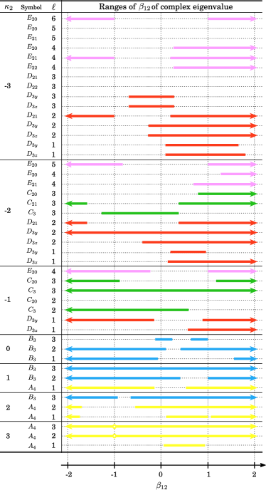
Figure 4: (Color online) Range of $\beta_{12}$ for complex eigenvalues in each $(\kappa_{1}=3,\kappa_{2},\ell)$.

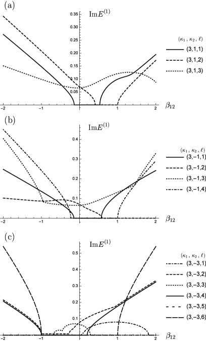
Figure 5: Maximum value of the imaginary parts of $E^{(1)}$ in units of $m\omega F$ for (a) $(\kappa_{1},\kappa_{2})=(3,1)$ with $\ell=1\,\sim\,3$ , (b) $(\kappa_{1},\kappa_{2})=(3,-1)$ with $\ell=1\,\sim\,4$, and (c) $(\kappa_{1},\kappa_{2})=(3,-3)$ with $\ell=1\,\sim\,6$ .

We can identify some general conclusions from Fig. 4. The co-rotating systems tend to be dynamically unstable. Most of the degenerate sets have wide ranges of $\beta_{12}$ with complex eigenvalues. The behaviors of counter-rotating systems of the two vortices are more complicated because the number of degenerate sets at each $(\kappa_{1},\kappa_{2},\ell)$ is two or more. For doubly degenerate sets, i.e. C_2n, D_2n, and $E_{2n}$ in Fig. 4, some complex eigenvalues appear away from $\beta_{12}=0$, while only real eigenvalues appear for some $(\kappa_{1},\kappa_{2},\ell)$ . Thus, the sign of $\beta_{12}$ is not essential, but positive $\beta_{12}$ is more likely to result in complex eigenvalues. Ranges without complex eigenvalue exist in subregion $E$ over small $|\beta_{12}|$ . This fact is consistent with the interpretation that decays of the two counter-rotating vortices are accelerated by energy exchange between the vortices through inter-component interaction. On the other hand, we also find stabilization due to the inter-component interaction. A weakly interacting system of a single vortex with winding number $\kappa$, which corresponds to the limiting case of $\beta_{12}=0$ in our formulation, gives complex eigenvalues for some $\ell$ and is dynamically unstable when $|\kappa|\geq 2$ Nakamura1 ; Pu . It is remarkable that there are a few ranges of $\beta_{12}$ where no complex eigenvalues arise (Fig. 4), explicitly $0.24\leq\beta_{12}\leq 0.42$ for $\kappa_{2}=0$ and $-1.0\leq\beta_{12}\leq-0.69$ for $\kappa_{2}=-3$.

Note that some of our results for $\kappa_{2}=-\kappa_{1}$ differ from those in Ref. Ishino , which were obtained by numerically solving the differential equations. However, the results are not inconsistent because the coupling constant $g$ in Ref. Ishino is much larger than that in our perturbative method.

IV.6 Splitting Patterns of Vortices

Let us next consider the splitting patterns of vortices according to the method of Ref. Kawaguchi .

Because the zeroth-order degeneracy of interest is quartic at the highest, we may express the zeroth-order eigenfunction with a fixed $\ell$, which may involve complex eigenvalues at the first order as

$$\bm{u}_{\ell}=c_{y1}\bm{y}_{n_{1}\ell 1}+c_{z1}\bm{z}_{n_{1}^{\prime}\ell 1}+c_{y2}\bm{y}_{n_{2}\ell 2}+c_{z2}\bm{z}_{n_{2}^{\prime}\ell 2}\,,$$ (60)

where the $c$ coefficients are determined from the eigenequation for $T^{\prime}_{\ell}$. One or two of $c$ coefficients are zero for triple or double degeneracy in the subregions B–E. When a mode associated with the eigenfunction $\bm{u}_{\ell}$ is excited, the change in the $j$-component order parameter is, for example,

$$\delta\psi_{\ell j}\propto c_{yj}\phi_{n_{j}\ell j}+c_{zj}\phi_{n_{j}-\ell j}^{*}\,,$$ (61)

which grows exponentially in time. Then, the condensate density of the $j$-component deforms as

$$|\psi_{j}+\delta\psi_{\ell j}|^{2}\simeq|\psi_{j}|^{2}+2\mathrm{Re}\psi^{*}_{j}\delta\psi_{\ell j}\,,$$ (62)

which has an $\ell$-fold rotational symmetry.

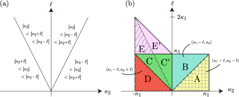
Figure 6: (Color online) (a) Magnitude relationship among $|\kappa_{2}-\ell|$, $|\kappa_{2}+\ell|$, and $|\kappa_{2}|$. The region is divided into four areas by the lines $\kappa_{2}=0$ and $\ell=\pm 2\kappa_{2}$. (b) Diagram of the splitting patterns of the vortices. The pattern of the resultant winding numbers after splitting of the initial $(\kappa_{1},\kappa_{2})$ are classified into three shaded areas.

The asymptotic form of the $j$th-component order parameter in the limit of $\rho\to 0$ is controlled by the winding number $\kappa_{j}$ as $\xi_{j}\sim\rho^{|\kappa_{j}|}$  . Inversely, the exponent of the asymptotic form of the order parameter informs the winding number. Because the asymptotic form of $\phi_{n\ell j}$ is proportional to $\rho^{|\kappa_{j}+\ell|}$, the winding number of the $j$th-component vortex with exponential growth results in $|\kappa_{j}\pm\ell|$ or remains $|\kappa_{j}|$. This restriction on the change in $\kappa_{j}$ is crucial. For $j=1$, we always have $|\kappa_{1}-\ell|<|\kappa_{1}|<|\kappa_{1}+\ell|$. The restriction for $j=2$ is depicted in Fig. 6 (a). Combining these results with Fig. 2, we finally obtain the splitting diagram shown in Fig. 6 (b). For example, in subregion A, it is predicted that the winding numbers of the two vortices vary from $(\kappa_{1},\kappa_{2})\to(\kappa_{1}-\ell,\kappa_{2}-\ell)$ once complex eigenvalues arise because $|\kappa_{j}-\ell|$ are the smallest in A. At first glance, we may conclude that the winding numbers also change into $(\kappa_{1}-\ell,\kappa_{2}-\ell)$ in subregion B, but this is not true. The correct answer is $(\kappa_{1}-\ell,\kappa_{2})$ because $\bm{z}_{n\ell 2}$ is not a member of the triply degenerate set in subregion B [see Table 1]. Subregions C and E are divided into two respective areas by the line $\ell=-2\kappa_{2}$.

V Summary

In this study, we searched for the dynamical instability parameter regions of a two-component system with coaxial quantized vortices. Our analytical method applied perturbation with respect to the coupling constants. Without numerically solving the BdG or TDGP equations, we completely obtained the unstable parameter ranges under the restriction of small coupling constants. Our method consists of the following three steps. First, we list all double degeneracies between $\bm{y}_{n\ell j}$ and $\bm{z}_{n^{\prime}\ell j^{\prime}}$ at the unperturbed level, which is necessary for the emergence of complex eigenvalues at the first order of the perturbation. At this step, the unstable modes certainly satisfy $1\leq\ell\leq\kappa_{1}$ for the co-rotating system and $1\leq\ell\leq\kappa_{1}-\kappa_{2}$ for the counter-rotating system. Next, all multiple degeneracies involving both $\bm{y}$ and $\bm{z}$ are enumerated. The relevant region of the $\kappa_{2}$–$\ell$ plane for a fixed $\kappa_{1}$ is divided into the five subregions A–E, as shown in Table 1. Note that a variety of degeneracies appear in the two-component system; however, in the single-component system, only a double degeneracy is involved for each $\ell$, but no radial excitation (no $n\neq$ one) appears. Finally, we can determine whether the degeneracies raise complex eigenvalues by solving the secular equation within each candidate degenerate set. Because the inter-component interaction coupling constant $\beta_{12}$ is the most sensitive and interesting parameter, we have searched for the range of complex eigenvalues, and the results for $\kappa_{1}=3$ are shown in Figs. 4 and 5. There are no heavy numerical calculations required because our secure equation is not more than a quartic equation. Thus, even though the system is restricted to small coupling constants, we have swept a wide parameter space, finding all unstable ranges.

As expected, Fig. 4 shows that the co-rotating ($\kappa_{2}>0$) and counter-rotating ($\kappa_{2}<0$) systems produce distinctive unstable ranges. In the co-rotating case, the addition of the second vortex ($\kappa_{2}$) does not drastically change the situation in which the highly quantized single vortex $\kappa_{1}\geq 2$ is already unstable. On the contrary, the counter-rotating system shows complicated behavior because the relative velocity of the two superflows are so large that large excitation energy radial modes can be members of degenerate sets, and complex eigenvalues appear if energy exchange between the two fluid components is possible. As shown in Fig. 4, complex eigenvalues appear for $\ell$, which are larger than the winding numbers ( $\ell>\kappa_{1}\geq|\kappa_{2}|$), in subregion E. This tendency becomes more pronounced for the larger absolute value of the inter-component coupling $|\beta_{12}|$, which accelerates the energy exchange between two components. We have also found a few regions where inter-component coupling stabilized the system. Finally, we have estimated all possible splitting patterns of the vortices with the aid of the degenerate set and the asymptotic forms of their eigenfunctions.

Appendix A Function Related to the Zeroth-Order BdG Eigenfunction

We give a concrete expression of the function $R_{n\ell j}$ , from Eq. (38) of Subsect. IV.1,

$$R_{n\ell j}(\rho)=C_{n\ell j}e^{-\frac{1}{2}\rho^{2}}\rho^{|\ell+\kappa_{j}|}S^{|\ell+\kappa_{j}|}_{n}(\rho^{2})\,.$$ (63)

Here, $S^{\gamma}_{n}(x)$ is Sonine polynomial, defined by

$$S^{\gamma}_{n}(x)=\sum_{k=0}^{n}\frac{(-1)^{k}(n+\gamma)!}{(n-k)!(\gamma+k)!k!}x^{k}$$ (64)

with the orthonormal property,

$$\int^{\infty}_{0}S^{\alpha}_{m}(x)S^{\alpha}_{n}(x)x^{\alpha}e^{-x}\,dx=\frac{\Gamma(\alpha+n+1)}{n!}\delta_{mn}\,.$$ (65)

The normalization condition on $\phi_{n\ell j}$, Eq. (41), implying

$$\int_{0}^{\infty}\left|R_{n\ell j}(\rho)\right|^{2}\,rdr=1\,,$$ (66)

fixes the normalization factor,

$$C_{n\ell j}=\sqrt{\frac{2m\omega\,n!}{(n+|\ell+\kappa_{j}|)!}}\,.$$ (67)

References

- (1) Y. Shin, M. Saba, M. Vengalattore, T. A. Pasquini, C. Sanner, A. E. Leanhardt, M. Prentiss, D. E. Pritchard, and W. Ketterle, Phys. Rev. Lett. 93, 160406 (2004).
- (2) L. Fallani, L. De Sarlo, J. E. Lye, M. Modugno, R. Saers, C. Fort, and M. Inguscio, Phys. Rev. Lett. 93, 140406 (2004).
- (3) F. Dalfovo, S. Giorgini, L. P. Pitaevskii, and S. Stringari, Rev. Mod. Phys. 71, 463 (1999).
- (4) J. A. M. Huhtamäki, M. Möttönen, T. Isoshima, V. Pietilä, and S. M. M. Virtanen, Phys. Rev. Lett. 97, 110406 (2006).
- (5) A. M. Mateo and V. Delgado, Phys. Rev. Lett. 97, 180409 (2006).
- (6) N. N. Bogoliubov, J. Phys. (Moscow) 11, 23 (1947).
- (7) P. G. de Gennes, Superconductivity of Metals and Alloys (Benjamin, New York, 1966).
- (8) A. L. Fetter, Ann. of Phys. 70, 67 (1972).
- (9) D. V. Skryabin, Phys. Rev. A 63, 013602 (2000).
- (10) S. Ishino, M. Tsubota, and H. Takeuchi, Phys. Rev. A 88, 063617 (2013).
- (11) L. Wen, Y. Qiao, Y. Xu, and L. Mao, Phys. Rev. A. 87, 033604 (2013).
- (12) Y. Kawaguchi and T. Ohmi, Phys. Rev. A. 70, 043610 (2004).
- (13) M. Mine, M. Okumura, T. Sunaga, and Y. Yamanaka, Ann. Phys. (N.Y.) 322, 2327 (2007).
- (14) E. Taylor and E. Zaremba, Phys. Rev. A 68, 053611 (2003).
- (15) E. Lundh and H. M. Nilsen, Phys. Rev. A. 74, 063620 (2006).
- (16) Y. Nakamura, M. Mine, M. Okumura, and Y. Yamanaka, Phys. Rev. A 77, 043601 (2008).
- (17) J. Takahashi, Y. Nakamura, and Y. Yamanaka, Ann. Phys. 347, 250 (2014).
- (18) H. Pu, C. K. Law, J. H. Eberly, and N. P. Bigelow, Phys. Rev. A 59, 1533 (1999).