Singular limit analysis of a model for earthquake faulting

Abstract

In this paper we consider a one dimensional spring-block model describing earthquake faulting. By using geometric singular perturbation theory and the blow-up method we provide a detailed description of the periodicity of the earthquake episodes. In particular we show that the limit cycles arise from a degenerate Hopf bifurcation whose degeneracy is due to an underlying Hamiltonian structure that leads to large amplitude oscillations. We use a Poincaré compactification to study the system near infinity. At infinity the critical manifold loses hyperbolicity with an exponential rate. We use an adaptation of the blow-up method to recover the hyperbolicity. This enables the identification of a new attracting manifold that organises the dynamics at infinity. This in turn leads to the formulation of a conjecture on the behaviour of the limit cycles as the time-scale separation increases. We illustrate our findings with numerics and suggest an outline of the proof of this conjecture.

Keywords: singular perturbation; Hamiltonian systems; rate and state friction; blow-up; earthquake dynamics; Poincaré compactification

1 Introduction

Earthquake events are a non-linear multi-scale phenomenon. Some of the non-linear occurrences are fracture healing, repeating behaviour and memory effects [Ruina1983, heaton1990a, vidale1994a, Marone1998]. In this paper we focus on the repeating behaviour of the earthquake cycles, where a cycle is defined as the combination of a rupture event with a following healing phase. An earthquake rupture consists of the instantaneous slipping of a fault side relative to the other side. The healing phase allows the fault to strengthen again and this process evolves on a longer time scale than the rupture event [carlson1989a, marone1998a].

The repetition of the earthquake events is significant for the predictability of earthquake hazards. The data collected in the Parkfield experiment in California show evidence of recurring micro-earthquakes [Nadeau1999, Marone1995, bizzarri2010a, Zechar2012]. For large earthquakes it is harder to detect a repeating pattern from the data, even though recent works indicate the presence of recurring cycles [Ben-zion2008].

The one dimensional spring-block model together with the empirical Ruina friction law is a fundamental model to describe earthquake dynamics [Burridge1967, Ruina1983, rice1983a, gu1984a, rice1986a, carlson1991a, belardinelli1996a, fan2014a]. Although the model does not represent all the non-linear phenomena of an earthquake rupture, it still reproduces the essential properties of the fault dynamics as extrapolated from experiments on rocks. The dimensionless form of the model is:

$$\dot{x} =-\rme^{z}\left(x+(1+\alpha)z\right),$$ (1)

$$\dot{y} =\rme^{z}-1,$$

$$\varepsilon\dot{z} =-\rme^{-z}\left(y+\frac{x+z}{\xi}\right).$$

Numerically, it has been observed that (1) has periodic solutions corresponding to the recurrence of the earthquake episodes, as shown in Figure 1 for two different values of the parameter $\varepsilon$ and $\alpha>\xi$ fixed. The steep growth of the $y$-coordinate corresponds to the earthquake rupture, while the slow decay corresponds to the healing phase. Hence the periodic solutions of (1) have a multiple time-scale dynamics. Furthermore in Figure 1 we observe that the amplitude of the oscillations increases for decreasing values of the time-scale separation $\varepsilon$. For these reasons extensive numerical simulations are difficult to perform in the relevant parameter range, that is $\varepsilon\in[10^{-24},10^{-8}]$ [rice1986a, carlson1989a, madariaga1996a, lapusta2000a, Erickson2008, Erickson2011].

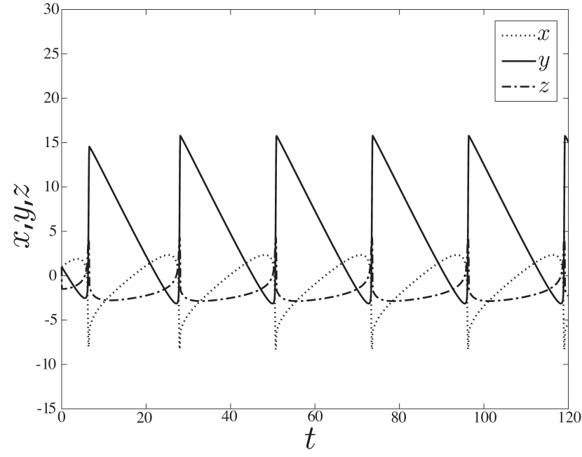
(a)

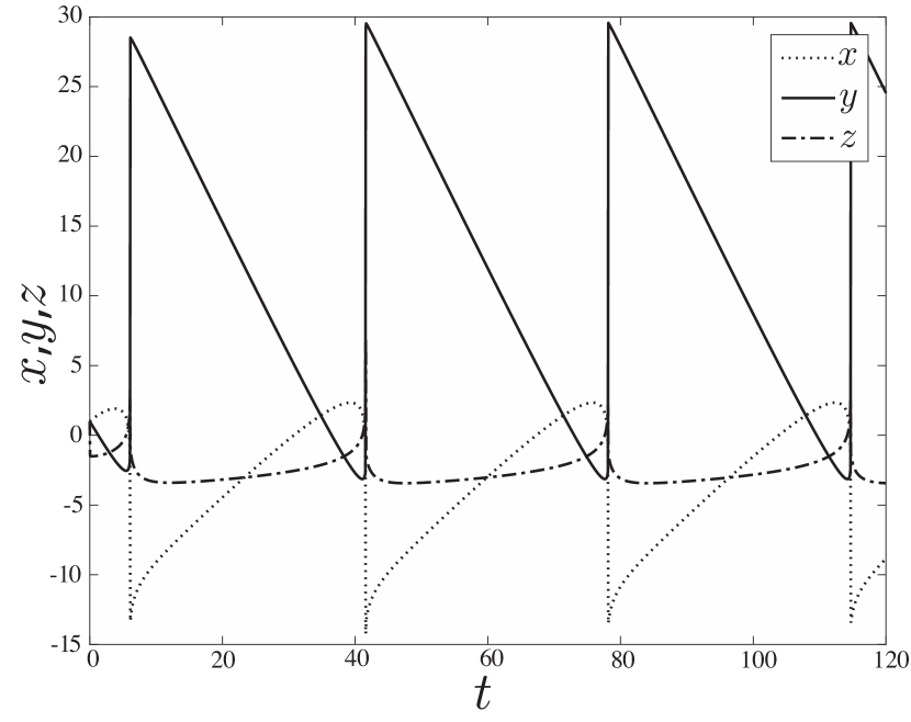
(b)

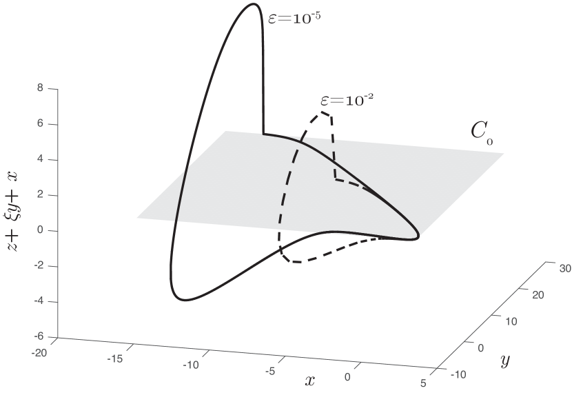
(c)

Figure 1: Numerical simulations of (1) for $\alpha=0.9$ and $\xi=0.5$. $\varepsilon=10^{-2}$ in 1(a) while $\varepsilon=10^{-5}$ in 1(b). In 1(c) phase space of both simulations. The grey plane $C_{0}$ and the coordinate $z+\xi y+x$ are clarified in section 3.

We remark that the periodic solutions of (1) appear in a finite interval of values of $\alpha>\xi$. If $\alpha$ is much larger than $\xi$ then chaotic dynamics emerges, as documented by Erickson2008 Erickson2008.
It is the purpose of the present paper to initiate a rigorous mathematical study of (1) as a singular perturbation problem [Jones1995, Kaper1999]. At the singular limit $\varepsilon=0$ we find an unbounded singular cycle when $\alpha>\xi$. For $\varepsilon>0$ we conjecture this cycle to perturb into a stable, finite amplitude limit cycle that explains the behaviour of Figure 1. In this way we can predict the periodic solutions of (1) even in parameter regions that are not possible to explore numerically. We expect that the deeper understanding of (1) that we provide, together with the techniques that we introduce, can be of help to study the continuum formulation of the Burridge and Knopoff model, in particular regarding the analysis of the Heaton pulses [heaton1990a].

As we will see in section 3, in our analysis the critical manifold loses normal hyperbolicity at infinity with an exponential rate. This is a non-standard loss of hyperbolicity that also appears in other problems [rankin2011a]. To deal with this issue we will first introduce a compactification of the phase space with the Poincaré sphere [chicone2006a] and repeatedly use the blow-up method of dumortier1996a dumortier1996a in the version of Krupa2001 Krupa2001. In particular we will use a technique that has been recently analyzed in [Kristiansen2015a]. For an introduction to the blow-up method we refer to [Kuehn2015].

Another way to study system (1) when $\varepsilon\ll 1$ is by using the method of matched asymptotic expansions, see [eckhaus1973a] for an introduction. putelat2008a putelat2008a have done the matching of the different time scales of (1) with an energy conservation argument, while in [pomeau2011critical] the causes of the switch between the two different time scales are not studied. However, the relaxation oscillation behavior of the periodic solutions of (1) is not explained.

Our paper is structured as follows. In section 2 we briefly discuss the physics of system (1). In section 3 we set (1) in the formalism of geometric singular perturbation theory and in section 4 we consider the analysis of the reduced problem for $\alpha=\xi$ and $\varepsilon=0$. Here a degenerate Hopf bifurcation appears whose degeneracy is due to an underlying Hamiltonian structure that we identify. We derive a bifurcation diagram in section 5 after having introduced a compactification of the reduced problem. From this and from the analysis of section 6, we conclude that the limit cycles of Figure 1 cannot be described by the sole analysis of the reduced problem. In section 7 we define a candidate singular cycle $\Gamma_{0}$ that is used in our main result, Conjecture 7.1. This conjecture is on the existence of limit cycles $\Gamma_{\varepsilon}\to\Gamma_{0}$ for $\varepsilon\ll 1$. The conjecture is supported by numerical simulations but in sections 8 and 9 we also lay out the foundation of a proof by using the blow-up method to gain hyperbolicity of $\Gamma_{0}$. Finally in section 10 we conclude and summarize the results of our analysis.

2 Model

The one dimensional spring-block model is presented in Figure 2. We suppose that one fault side slides at a constant velocity $v_{0}$ and drags the other fault side of mass $M$ through a spring of stiffness $\kappa$. The friction force $F_{\mu}=\sigma\mu$ acts against the motion. A common assumption is to suppose that the normal stress $\sigma$, i.e. the stress normal to the friction interface [Nakatani2001], is constant $\sigma=1$. The friction coefficient $\mu$ is modelled with the Ruina rate and state friction law $\mu=\mu(v,\theta)$, with $v$ the sliding velocity and $\theta$ the state variable. The state $\theta$ accounts for how long the two surfaces have been in contact [Ruina1983, Marone1998].

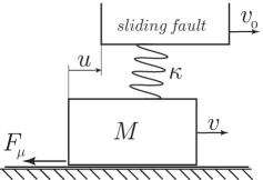
Figure 2: Spring-block model describing the earthquake faulting.

The equations of our model are:

$${\theta}^{\prime} =-\frac{v}{L}\left(\theta+b\ln\left(\frac{v}{v_{0}}\right)\right),$$ (2)

$${u}^{\prime} =v-v_{0},$$

$$M{v}^{\prime} =-\kappa u-\left(\theta+a\ln\left(\frac{v}{v_{0}}\right)\right),$$

where the variable $u$ is the relative displacement between the two fault sides and the prime denotes the time derivative. The parameter $L$ is the characteristic displacement that is needed to recover the contact between the two surfaces when the slip occurs, while $a$ and $b$ are empirical coefficients that depend on the material properties [Marone1998]. We introduce the dimensionless coordinates $(x,y,w,t)$ into system (2), where $\theta=ax,\,\,u=Ly,\,\,v=v_{0}w,\,\,t=({v_{0}}/L)t^{\prime}$:

$$\dot{x} =-w\left(x+(1+\alpha)\ln(w)\right),$$ (3)

$$\dot{y} =w-1,$$

$$\varepsilon\dot{w} =-y-\frac{x+\ln(w)}{\xi}.$$

We notice that equation (3) has a singularity in $w=0$ and to avoid it we henceforth introduce the variable $z=\ln(w)$ so that we obtain the formulation presented in (1). In system (3) we have introduced the parameters: $\varepsilon=Mv_{0}^{2}/(\kappa L^{2})$ such that $1/\sqrt{\varepsilon}$ is a non-dimensional frequency, $\xi=(\kappa L)/a$: the non-dimensional spring constant and $\alpha=(b-a)/b$ describing the sensitivity to the velocity relaxation [Erickson2008]. We consider the parameter values presented by Madariaga1998 Madariaga1998: $\varepsilon\in[10^{-24},10^{-8}]$, $\xi=0.5$, $\alpha>\xi$. An extensive reference to the parameter sets is in the work of dieterich1972 dieterich1972,dieterich1978a,Dieterich1979. We choose to keep the parameter $\xi>0$ fixed (selecting $\xi=0.5$ in our computations) and we use $\alpha$ as the bifurcation parameter. With this choice the study of (1) as a singular perturbation problem is simplified. Indeed as we will see in section 3, the critical manifold of (1) is a surface that depends on $\xi$. The results of our analysis can be easily interpreted for the case of $\alpha$ fixed and $\xi$ varying, that is the standard approach in the literature.

3 Singular perturbation approach to the model

The positive constant $\varepsilon\ll 1$ in system (1) measures the separation of two time scales. In particular the variables $(x,y)$ are slow while $z$ is fast. We call equation (1) the slow problem and the dot refers to the differentiation with respect to the slow time $t$. We introduce the fast time $\tau=t/\varepsilon$ to obtain the fast problem:

$$x^{\prime} =-\varepsilon\rme^{z}(x+(1+\alpha)z),$$ (4)

$$y^{\prime} =\varepsilon\left(\rme^{z}-1\right),$$

$$z^{\prime} =-\rme^{-z}\left(y+\frac{x+z}{\xi}\right),$$

where the prime stands for differentiation with respect to $\tau$. The two systems (1) and (4) are equivalent whenever $\varepsilon>0$. In the singular analysis we consider two different limit systems. By setting $\varepsilon=0$ in (1) we obtain the reduced problem:

$$\dot{x} =-\rme^{z}(x+(1+\alpha)z),$$ (5)

$$\dot{y} =\rme^{z}-1,$$

$$0 =-\rme^{-z}\left(y+\frac{x+z}{\xi}\right),$$

that is also referred in the literature as the quasi-static slip motion (specifically $M\to 0$ in (2), [Ruina1983]). Setting $\varepsilon=0$ in (4) gives the layer problem:

$${z}^{\prime}=-\rme^{-z}\left(y+\frac{x+z}{\xi}\right),\quad(x,y)(\tau)=(x^{0},y^{0}).$$ (6)

System (6) has a plane of fixed points that we denote the critical manifold:

$$C_{0}:=\Bigl{\{}(x,y,z)\in\mathbb{R}^{3}\Bigr{|}\quad z=-x-\xi y\Bigr{\}}.$$ (7)

This manifold, depicted in grey in Figure 1(c), is attracting:

$$\frac{\partial{z}^{\prime}}{\partial z}\biggr{|}_{C_{0}}=-\xi^{-1}\rme^{-z}<0.$$ (8)

The results by fenichel1974a fenichel1974a,Fenichel1979 guarantee that close to $C_{0}$ there is an attracting (due to (8)) slow-manifold $S_{\varepsilon}$ for any compact set $(x,y)\in\mathbb{R}^{2}$ and $\varepsilon$ sufficiently small. However we notice in (8) that $C_{0}$ loses its normal hyperbolicity at an exponential rate when $z\to+\infty$. This is a key complication: orbits leave a neighborhood of the critical manifold even if it is formally attracting. This is a non-standard loss of hyperbolicity that appears also in other physical problems [rankin2011a]. To our knowledge, [Kristiansen2015a] is the first attempt on a theory of exponential loss of hyperbolicity. In section 8 we will apply the method described in [Kristiansen2015a] to resolve the loss of hyperbolicity at infinity. In this paper we do not aim to give a general geometric framework to this approach. In the case of loss of hyperbolicity at an algebraic rate, like in the autocatalator problem studied originally by Gucwa2009783 Gucwa2009783, we refer to the work of kuehn2014a kuehn2014a.
Naïvely we notice that when $z\gg 1$ the dynamics of system (1) is driven by a new time scale, that is not related to its slow-fast structure. Assuming $z\gg\ln\varepsilon^{-1}$ we can rewrite (1) as:

$$\dot{x} =-x-(1+\alpha)z,$$ (9)

$$\dot{y} =1,$$

$$\dot{z} =0,$$

where we have further rescaled the time by dividing the right hand side by $\rme^{z}$ and ignored the higher order terms. Hence in this regime there is a family of $x$-nullclines:

$$x+(1+\alpha)z=0,$$ (10)

that are attracting since:

$$\frac{\partial\dot{x}}{\partial x}=-1.$$

This naïve approach is similar to the one used by rice1986a rice1986a to describe the different time scales that appear in system (1).

4 Reduced Problem

We write the reduced problem (5) as a vector field $f_{0}(y,z;\alpha)$ by eliminating $x$ in (5):

$$f_{0}(y,z;\alpha):=\quad\begin{cases}\dot{y}&=\rme^{z}-1,\\ \dot{z}&=\xi+\rme^{z}\left(\alpha z-\xi y-\xi\right).\end{cases}$$ (11)

The following proposition describes the degenerate Hopf bifurcation at the origin of (11) for $\alpha=\xi$.

Proposition 4.1

The vector field (11) has a unique fixed point in $(y,z)=(0,0)$ that undergoes a degenerate Hopf bifurcation for $\alpha=\xi$. In particular $f_{0}(y,z;\xi)$ is Hamiltonian and it can be rewritten as:

$$f_{0}(y,z;\xi)=g(y,z)J\nabla H(y,z),$$ (12)

with

$$g(y,z) =\frac{\rme^{\xi y+z}}{\xi},$$ (13a)

$$H(y,z) =-\rme^{-\xi y}\left(\xi y-\xi z+\xi+1-\xi\rme^{-z}\right)+1,$$ (13b)

and where $J$ is the standard symplectic structure matrix: $J=\begin{bmatrix}0&1\\ -1&0\end{bmatrix}.$

• The linear stability analysis of (11) in the fixed point $(y,z)=(0,0)$ gives the following Jacobian matrix:

  $$Df_{0}(0,0;\alpha)=\begin{bmatrix}0&1\\ -\xi&\alpha-\xi\end{bmatrix}.$$ (14)

  The trace of (14) is zero for $\alpha=\xi$ and its determinant is $\xi>0$. Hence a Hopf bifurcation occurs. The direct substitution of (13) into (12) shows that system (11) is Hamiltonian for $\alpha=\xi$. Therefore the Hopf bifurcation is degenerate. $\Box$

(a)

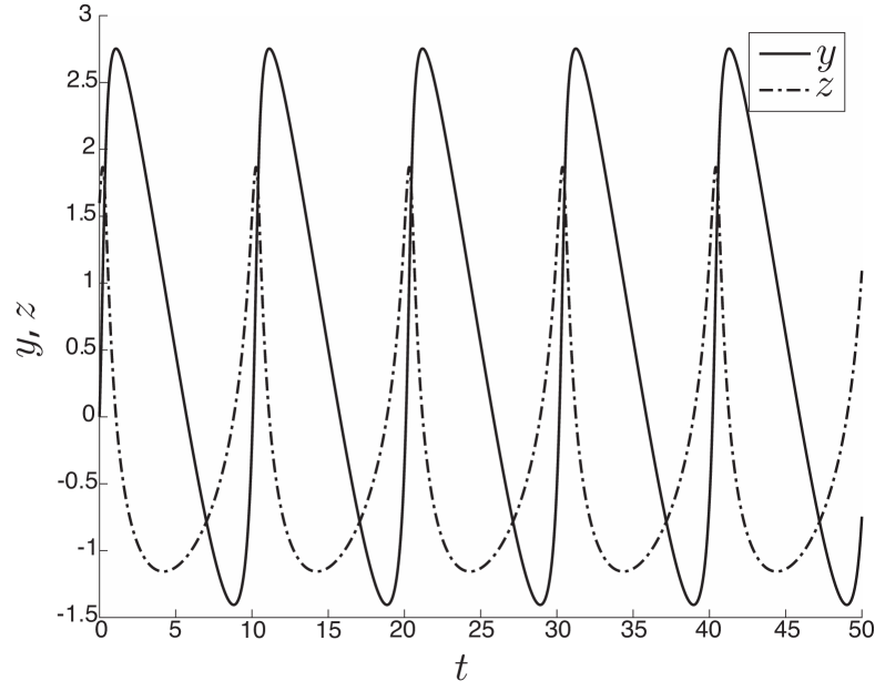
(b)

Figure 3: Behaviour of the reduced problem (12) for $\alpha=\xi$. In 3(a): phase space. The axis orientation is chosen in order to be consistent with the remaining figures of the paper. In 3(b): simulation of (12) for $H=0.4,\,\,\xi=0.5$.

The Hopf bifurcation of (11) for $\alpha=\xi$ is a known result [Ruina1983, putelat2008a, Erickson2008]. The function $H(y,z)$ has been used as a Lyapunov function in [gu1984a] without realising the Hamiltonian structure of (11).
From Proposition 4.1 we obtain a vertical family of periodic orbits for $\alpha=\xi$. The phase space of (12) is illustrated in Figure 3(a) for positive values of $H(y,z)$. We remark that the fixed point $(y,z)=(0,0)$ is associated with $H(y,z)=0$.
The intersection of the $y$-axis with the orbits $H(y,z)=h$ corresponds to the real roots of the Lambert equation:

$$-\rme^{-\xi y}(\xi y+1)+1=h,\quad h\geq 0.$$ (15)

Equation (15) has a real root for any $h>0$ in the region $y<0$, while a second real root in the region $y>0$ exists only for $h\in(0,1)$ [corless2014a]. The intersection of the Hamiltonian trajectories with the $y$-axis is transversal for all $h>0$, since the following condition holds:

$$\frac{\partial H}{\partial y}(y,0)=\xi^{2}y\rme^{-\xi y}\neq 0,\quad\forall y\neq 0.$$ (16)

The trajectory identified with $H(y,z)=1$ (that is in bold in Figure 3(a)) plays a special role since it separates the closed orbits for $H\in(0,1)$ from the unbounded ones for $H\geq 1$. Our analysis supports the results of gu1984a gu1984a and contrasts [ranjith1999a] where it is claimed that (12) has no unbounded solutions.

Remark 1

From (16) it follows that the function $H(y,0)$ defines a diffeomorphism between the points on the positive $y$-axis and the corresponding values $h\in(0,1)$.

Figure 3(b) highlights that the reduced problem (12) has an intrinsic slow-fastness. Indeed the phase space of (12) is swept with different speeds depending on the region considered. This feature is represented in Figure 3(a), with the double arrow representing fast motion. In particular when $z>0$ the trajectories are swept faster than for $z<0$. This is due to the exponential function in (11). The fast sweep for $z>0$ corresponds to the steep increase in the $y$ coordinate of Figure 3(b). This fast dynamics for $z>0$ resembles the slip that happens during an earthquake rupture, while the slow motion for $z<0$ matches the healing phase, recall Figure 1. From this observation we tend to disagree with the notation used in the literature, that calls the reduced problem the quasi-static slip phase [Ruina1983].
In order to describe the unbounded trajectories with $H(y,z)\geq 1$ for $y,z\to\infty$ and to extend the analysis to the case $\alpha\neq\xi$, we introduce a compactification of the reduced problem (11) and then we rewrite (11) on the Poincaré sphere.

5 Compactification of the reduced problem

We define the Poincaré sphere $\mathcal{S}^{2,+}$ as:

$$\mathcal{S}^{2,+}:=\{(Y,Z,W)\in\mathbb{R}^{3}\bigr{|}\quad Y^{2}+Z^{2}+W^{2}=1,\quad W\geq 0\},$$ (17)

which projects the phase space of (11) onto the northern hemisphere of $\mathcal{S}^{2,+}$. We refer to [chicone2006a] for further details on the compactification of vector fields. Geometrically (17) corresponds to embedding (11) into the plane $W=1$ that we call the directional chart $k_{2}$:

$$k_{2}:=\mathcal{S}^{2,+}\cap\{W=1\},\quad y_{2}=\frac{Y}{W},\,\,z_{2}=\frac{Z}{W},$$

and the dynamics on chart $k_{2}$ follows directly from (11) by variable substitution:

$$\dot{y}_{2} =\rme^{z_{2}}-1,$$ (18)

$$\dot{z}_{2} =\xi+\rme^{z_{2}}\left(\alpha z_{2}-\xi y_{2}-\xi\right).$$

The points at infinity in $k_{2}$ correspond to the condition $W=0$, that is the equator of $\mathcal{S}^{2,+}$. To study the dynamics on the equator we introduce the two additional directional charts:

$$k_{3}:=\mathcal{S}^{2,+}\cap\{Z=1\},\quad y_{3}=\frac{Y}{Z},w_{3}=\frac{W}{Z},$$ (19a)

$$k_{1}:=\mathcal{S}^{2,+}\cap\{Y=1\},\quad z_{1}=\frac{Z}{Y},w_{1}=\frac{W}{Y}.$$ (19b)

We follow the standard convention of Krupa2001 Krupa2001 and use the subscript $i=1,2,3$ to denote a quantity in chart $k_{i}$. We denote with $k_{ij}$ the transformation from chart $k_{i}$ to chart $k_{j}$ for $i,j=1,2,3$. We have the following change of coordinates:

$$k_{23}:\quad w_{3}=z_{2}^{-1},\quad y_{3}=y_{2}z_{2}^{-1},$$ (20a)

$$k_{21}:\quad w_{1}=y_{2}^{-1},\quad z_{1}=z_{2}y_{2}^{-1},$$ (20b)

$$k_{31}:\quad w_{1}=w_{3}y_{3}^{-1},\quad z_{1}=y_{3}^{-1},$$ (20c)

that are defined for $z_{2}>0$, $y_{2}>0$ and $y_{3}>0$ respectively. The inverse transformations $k_{ji}=k_{ij}^{-1}$ are defined similarly. Figure 4 shows a graphical representation of the sphere and the directional charts.
We define $C_{0,\infty}$ as the extension of the critical manifold $C_{0}$ onto the equator of the sphere. From (8) it follows that $C_{0,\infty}$ is non-hyperbolic.

Figure 4: Poincaré sphere $\mathcal{S}^{2,+}$ and the directional charts $k_{1,2,3}$.

Proposition 5.1

There exists a time transformation that is smooth for $W>0$ and that de-singularizes the dynamics within $W=0$, so that the reduced problem (11) has four fixed points $Q^{1,3,6,7}$ on $C_{0,\infty}$ satisfying:

• $Q^{1}$ is an improper stable node with a single eigenvector tangent to $C_{0,\infty}$.

• $Q^{3}$ has one unstable direction that is tangent to $C_{0,\infty}$ and a unique center-stable manifold $W^{c,s}$.

• $Q^{6}$ has one stable direction that is tangent to $C_{0,\infty}$ and a unique center-unstable manifold $W^{c,u}$.

• $Q^{7}$ is an improper unstable node with a single eigenvector tangent to $C_{0,\infty}$.

The stability properties of the fixed points are independent of $\alpha$, in particular both $W^{c,s}$ and $W^{c,u}$ are smooth in $\alpha$.

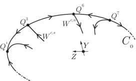
Figure 5: Fixed points on the compactified critical manifold $C_{0}$.

Figure 5 gives a representation of the statements of Proposition 5.1. We remark that we use superscripts as enumeration of the points $Q^{m},m=1,3,6,7$ to avoid confusion with the subscripts that we have used to define the charts $k_{i},i=1,2,3$. In particular the enumeration choice of the superscripts will become clear in section 7, where we will introduce the remaining points $Q^{2,4,5}$ in (53). In Proposition 5.2 we relate the structure at infinity of (11) to the dynamics on $C_{0}$ with respect to the parameter $\alpha$.

Proposition 5.2

Fix $c>0$ small and consider the parameter interval:

$$\alpha\in[\xi-c,\xi+c].$$ (21)

Then Figure 6 describes the phase space of (11) with respect to $\alpha$. In particular:

• When $\alpha<\xi$ the set $W^{c,s}$ separates the basin of attraction of $(y,z)=(0,0)$ from the solutions that are forward asymptotic to $Q^{1}$.

• When $\alpha=\xi$ Proposition 4.1 holds. The set $H=1$ corresponds to $W^{c,s}\cap W^{c,u}$.

• When $\alpha>\xi$ the set $W^{c,u}$ separates the solutions that are backwards asymptotic to the origin to the ones that are backwards asymptotic to $Q^{7}$.

Therefore no limit cycles appear in the reduced problem for $\varepsilon=0$ and $\alpha\neq\xi$.

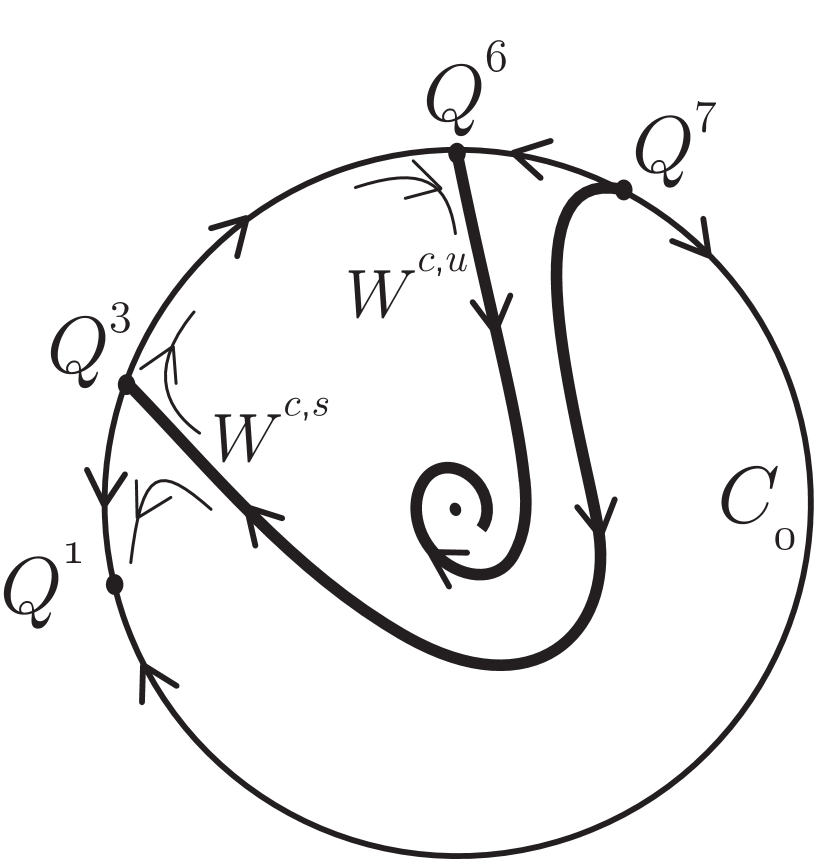
(a)

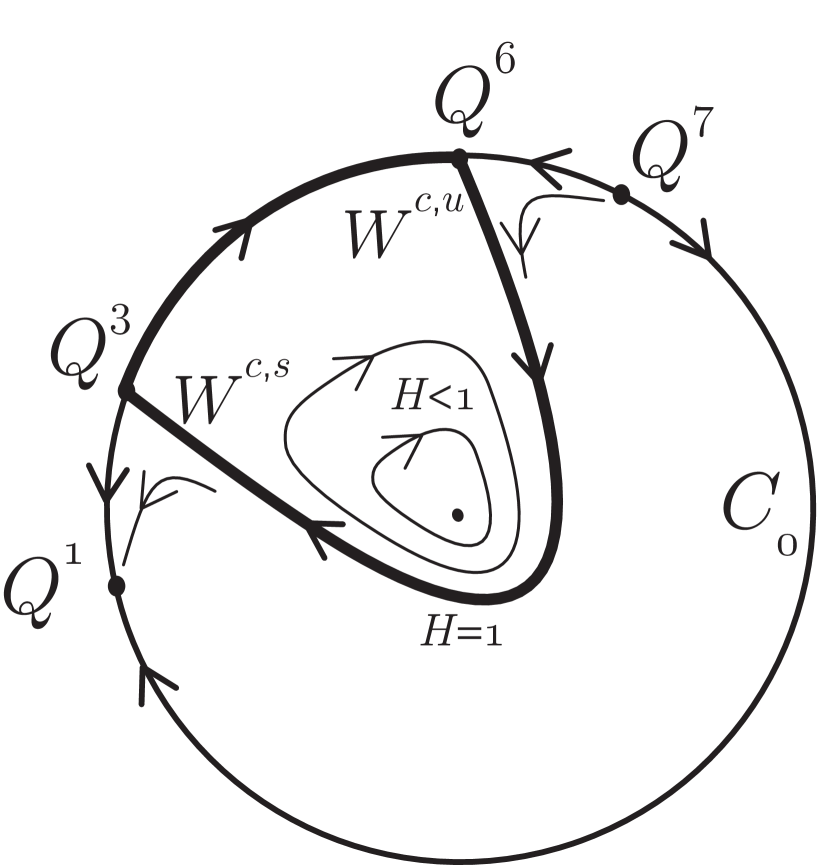
(b)

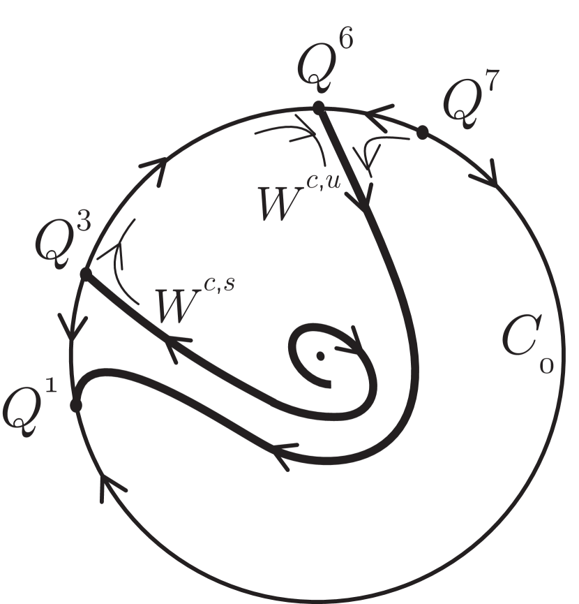
(c)

Figure 6: Bifurcation diagram of (11) with respect to the parameter $\alpha$. Orbits spiral inwards for $\alpha<\xi$ 6(a) or outwards for $\alpha>\xi$ 6(c). In 6(b): $\alpha=\xi$.

Remark 2

The local stability analysis of $(y,z)=(0,0)$ can be directly obtained using $H(y,z)$ as a Lyapunov function. This was done in [gu1984a].

In the rest of the section we prove the previous two propositions. In sections 5.1 and 5.2 we perform an analysis of (11) in the two charts $k_{3}$ and $k_{1}$ respectively to show Proposition 5.1. We prove Proposition 5.2 in section 5.3.

5.1 Chart $k_{3}$

We insert (19a) into the reduced problem (18) and obtain the following system:

$$\dot{w}_{3} =-w_{3}(\alpha-\xi y_{3})+\xi w_{3}^{2}(1-\rme^{-\frac{1}{w_{3}}}),$$ (22)

$$\dot{y}_{3} =-y_{3}(\alpha-\xi y_{3})-w_{3}(1+\xi y_{3})(1-\rme^{-\frac{1}{w_{3}}}),$$

here we have divided the right hand side by $\exp(1/w_{3})$ to de-singularize $w_{3}=0$.

Remark 3

The division by $\exp(1/w_{3})$ in (22) is formally performed by introducing the new time $t_{3}$ such that:

$$\rmd t_{3}=\exp(1/w_{3})\rmd t.$$ (23)

A similar de-singularization procedure is also used in the blow-up method.

System (22) has two fixed points:

$$Q^{1}:=\quad(w_{3},y_{3})=(0,0),$$ (24a)

$$Q^{3}:=\quad(w_{3},y_{3})=\left(0,\frac{\alpha}{\xi}\right).$$ (24b)

The point $Q^{1}$ is a stable improper node with the double eigenvalue $-\alpha$ and a single eigenvector $(0,1)^{T}$. The point $Q^{3}$ has one unstable direction $(0,1)^{T}$ due to the positive eigenvalue $\alpha$ and a center direction $(\alpha/(1+\alpha),1)^{T}$ due to a zero eigenvalue. Notice that for $\alpha=\xi$ then $Q^{3}=(0,1)$.

Lemma 5.3

There exists a unique center-stable manifold $W^{c,s}$ at the point $Q^{3}$. This manifold is smooth in $\alpha$. For $\alpha=\xi$ the set $H=1$ coincides with $W^{c,s}$.

• For $\alpha=\xi$ we rewrite the Hamiltonian (13b) in chart $k_{3}$ and insert the condition $H=1$ to obtain the implicit equation:

  $$\xi(y_{3}-1)+w_{3}(\xi+1)-\xi w_{3}\rme^{-\frac{1}{w_{3}}}=0,$$ (25)

  then $w_{3}\to 0$ gives $y_{3}\to 1$ that is the point $Q^{3}$. As a consequence $Q^{3}$ has a saddle-like behaviour with an unique center-stable manifold $W^{c,s}$ tangent to $(\alpha/(1+\alpha),1)^{T}$. This invariant manifold $W^{c,s}$ is smooth in $\alpha$ and therefore it preserves its features for small variations of $\alpha$ from $\alpha=\xi$. $\Box$

Remark 4

With respect to $t_{3}$ the points within $W^{c,s}$ decay algebraically to $Q^{3}$, while the decay towards the stable node $Q^{1}$ is exponential. Using (23) it then follows that all these points reach $w_{3}=0$ in finite time with respect to the original slow time $t$. This is a formal proof of the finite time blow-up of solutions of (11) for $\alpha>\xi$ that was also observed by gu1984a gu1984a and by pomeau2011critical pomeau2011critical.

5.2 Chart $k_{1}$

We insert (19b) into the reduced problem (18) to obtain the dynamics in chart $k_{1}$:

$$\dot{w} =w^{2}(1-\rme^{\frac{z}{w}}),$$ (26)

$$\dot{z} =w(\xi+z)(1-\rme^{\frac{z}{w}})+\rme^{\frac{z}{w}}(\alpha z-\xi),$$

where we have dropped the subscript for the sake of readability. We observe that the exponential term in (26) is not well defined in the origin. For this reason we introduce the blow-up transformation:

$$w=\bar{r}\bar{\omega},\qquad z=\bar{r}\bar{\zeta},$$ (27)

where $(\bar{\omega},\bar{\zeta})\in S^{1}=\{(\bar{\omega},\bar{\zeta}):\bar{\omega}^{2}+\bar{\zeta}^{2}=1\}$ and $\bar{r}\geq 0$. We consider the following charts:

$$\kappa_{1}:\quad w=r_{1}\omega_{1},\quad z=r_{1},$$ (28a)

$$\kappa_{2}:\quad w=r_{2},\qquad z=r_{2}\zeta_{2},$$ (28b)

$$\kappa_{3}:\quad w=r_{3}\omega_{3},\quad z=-r_{3}.$$ (28c)

Next we perform an analysis of the blown-up vector field and the main results are summarized in Figure 7.

Chart $\kappa_{1}$

We insert condition (28a) into system (26) and divide the right hand side by $\exp(1/\omega_{1})/r_{1}$ to get the de-singularized dynamics in chart $\kappa_{1}$:

$$\dot{\omega}_{1} =\omega_{1}(\xi-\alpha r_{1})+r_{1}\omega_{1}^{2}\xi\left(1-\rme^{-\frac{1}{\omega_{1}}}\right),$$ (29)

$$\dot{r}_{1} =-r_{1}(\xi-\alpha r_{1})-r_{1}^{2}\omega_{1}(\xi+r_{1})\left(1-\rme^{-\frac{1}{\omega_{1}}}\right).$$

System (29) has one fixed point in $(\omega_{1},r_{1})=(0,\xi/\alpha)$ that corresponds to the point $Q^{3}$ introduced in (24b). Furthermore system (29) has a second fixed point in $O_{1}:=(\omega_{1},r_{1})=(0,0)$ with eigenvalues $\xi,\,\,-\xi$ and corresponding eigenvectors $(1,0)^{T}$ and $(0,1)^{T}$. Both the eigendirections of $O_{1}$ are invariant and we denote by $\gamma_{1}$ the heteroclinic connection between $Q^{3}$ and $O_{1}$ along the $r_{1}$-axis.
The initial condition $p_{1,\text{in}}$ on $W^{c,s}$ with $\omega_{1}=\delta>0$ is connected through the stable and the unstable manifolds of $O_{1}$ to the point $p_{1,\text{out}}:=(\omega_{1},r_{1})=(\delta^{-1},0)$ as shown in Figure 7(a).

Chart $\kappa_{2}$

We insert the transformation (28b) into (26) and divide the right hand side by $\exp(\zeta_{2})/r_{2}$ to obtain the de-singularized vector field. In this chart there are no fixed points, yet the line $r_{2}=0$ is invariant and $\zeta_{2}$ decreases monotonically along it. The orbit entering from chart $\kappa_{1}$ has the initial condition $p_{2,\text{in}}:=\kappa_{12}(p_{1,\text{out}})=\,\,(\zeta_{2},r_{2})=(\delta,0)$ that lies on the invariant line $r_{2}=0$. Thus from $p_{2,\text{in}}$ we continue to the point $p_{2,\text{out}}:=(\zeta_{2},r_{2})=(-\delta^{-1},0)$, as shown in Figure 7(b).

Chart $\kappa_{3}$

We introduce condition (28c) into the vector field (26) and divide by $w_{3}$ to obtain the de-singularized dynamics in chart $\kappa_{3}$:

$$\dot{\omega}_{3} =(\xi-r_{3})(1-\rme^{-\frac{1}{\omega_{3}}})+r_{3}\omega_{3}(1-\rme^{-\frac{1}{\omega_{3}}})+\frac{\rme^{-\frac{1}{\omega_{3}}}}{r_{3}}(\alpha r_{3}+\xi),$$ (30)

$$\dot{r}_{3} =-r_{3}(\xi-r_{3})(1-\rme^{-\frac{1}{\omega_{3}}})-\frac{\rme^{-\frac{1}{\omega_{3}}}}{\omega_{3}}(\alpha r_{3}+\xi).$$

System (30) has an unstable improper node in:

$$Q^{7}:=\quad(\omega_{3},r_{3})=(0,\xi),$$ (31)

with double eigenvalue $\xi$ and single eigenvector $(1,0)^{T}$. For $w_{3}=r_{3}=0$ the quantity $\rme^{-1/\omega_{3}}/r_{3}$ in (30) is not well defined. We deal with this singularity by first multiplying the right hand side of the vector field by $r_{3}\omega_{3}$:

$$\dot{\omega}_{3} =r_{3}\omega_{3}(\xi-r_{3})(1-\rme^{-\frac{1}{\omega_{3}}})+r_{3}^{2}\omega_{3}^{2}(1-\rme^{-\frac{1}{\omega_{3}}})+\omega_{3}\rme^{-\frac{1}{\omega_{3}}}(\alpha r_{3}+\xi),$$ (32)

$$\dot{r}_{3} =-r_{3}^{2}\omega_{3}(\xi-r_{3})(1-\rme^{-\frac{1}{\omega_{3}}})-r_{3}\rme^{-\frac{1}{\omega_{3}}}(\alpha r_{3}+\xi).$$

Next we introduce the blow-up transformation:

$$\omega_{3}=\rho,\qquad r_{3}=\frac{\rme^{-1/\rho}}{\rho}\eta.$$ (33)

We substitute (33) into (32) and we divide by $\exp(-1/\rho)/\rho$ to obtain the de-singularized vector field:

$$\dot{\rho} =\xi\rho^{2}(\eta-1)+\Or\left(\frac{\eta}{\rho}\rme^{-1/\rho}\right),$$ (34)

$$\dot{\eta} =-\eta\xi(\eta-1)+\Or\left(\frac{\eta}{\rho}\rme^{-1/\rho}\right).$$

Remark 5

The blow-up map (33) is non-standard, since it is not written as an algebraic expression in $\rho$. To the author’s knowledge there is no former literature treating blow-ups of the form (33) and in particular the approach of [Kristiansen2015a] does not treat this type of blow-ups.

System (34) has two fixed points. The first fixed point $O_{3}:=(\rho,\eta)=(0,0)$ has one unstable direction $(0,1)^{T}$ associated with the eigenvalue $\xi$ and one center direction $(1,0)^{T}$ associated with the zero eigenvalue. The second fixed point is:

$$Q^{6}:=\quad(\rho,\eta)=(0,1),$$ (35)

and it has one stable direction $(0,1)^{T}$ associated with the eigenvalue $-\xi$ and one center direction $(1,0)^{T}$ associated with the zero eigenvalue. The axis $\rho=0$ is invariant, thus there exists an heteroclinic connection along the $\eta$-axis between the points $O_{3}$ and $Q^{6}$ that we denote by $\gamma_{3}$, see Figure 7(c).

Lemma 5.4

There exists a unique center-unstable manifold $W^{c,u}$ at the point $Q^{6}$ that is smooth in $\alpha$ and that contains solutions that decay algebraically to $Q^{6}$ backwards in time. For $\alpha=\xi$ the set $H=1$ coincides with $W^{c,u}$.

• We rewrite the Hamiltonian (13b) in the $(\rho,\eta)$ coordinates and then insert the condition $H=1$ to obtain the implicit equation:

  $$\frac{1}{\eta}-1+\rme^{-\frac{1}{\rho}}\left(\frac{1}{\rho}+1+\frac{1}{\xi}\right)=0.$$ (36)

  Here $\rho\to 0$ gives $\eta\to 1$. Therefore $Q^{6}$ has a saddle-like behaviour with a unique center-unstable manifold $W^{c,u}$ that is tangent to $(1,0)^{T}$ in $Q^{6}$. The invariant manifold $W^{c,u}$ is smooth in $\alpha$ and it maintains the center-unstable properties for small variation of $\alpha$ from $\alpha=\xi$. $\Box$

The orbit entering from chart $\kappa_{2}$ in the point $p_{3,\text{in}}:=\kappa_{23}(p_{2,\text{out}})=(\rho,\eta)=(\delta,0)$ is connected through the stable and the unstable manifolds of $O_{3}$ to the point $p_{3,\text{out}}$ on $W^{c,u}$ with $\omega_{3}=\delta$ as shown in Figure 7(c).

Remark 6

We observe that the singularity at the origin of chart $k_{1}$ (26), upon blow-ups (27) and (33), has turned into three hyperbolic fixed points $O_{1},O_{3}$ and $Q^{6}$. After the blow-down we obtain the singular structure depicted in Figure 7(d).

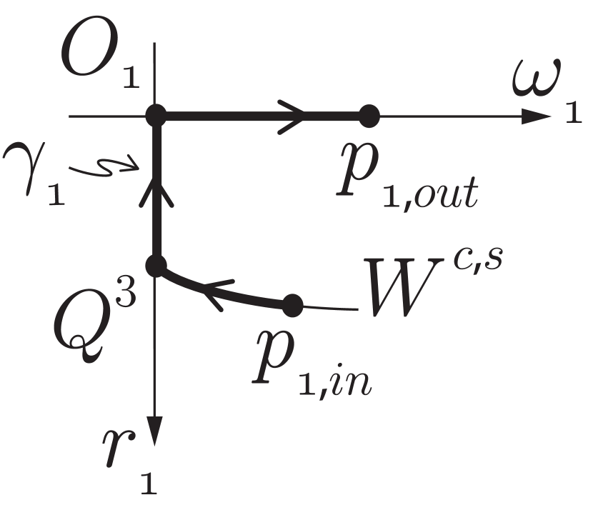
(a)

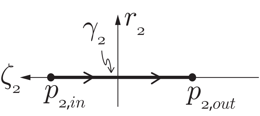
(b)

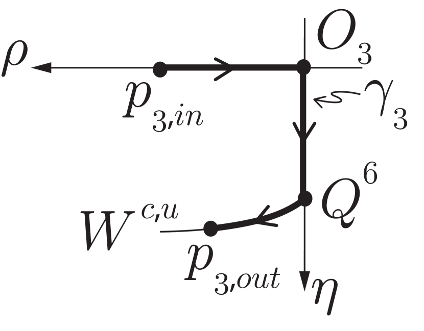
(c)

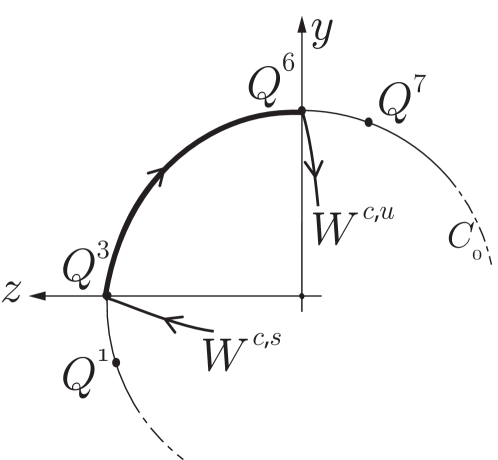
(d)

Figure 7: Blow-up of (26) in chart $k_{1}$. 7(a), 7(b) and 7(c) represent charts $\kappa_{1},\kappa_{2}$ and $\kappa_{3}$ respectively. In 7(d): behaviour at infinity after the blow-down.

5.3 The reduced problem on $\mathcal{S}^{2,+}$

The previous analysis has described the phase space of (11) near infinity. In the following we analyse the interaction of the unbounded solutions of the reduced problem (11) with the fixed points $Q^{1,3,6,7}$ for variations of the parameter $\alpha$. We follow the Melnikov-type approach of Chow94 Chow94, to describe how the closed orbits of the Hamiltonian system (12) break up near $\alpha=\xi$.
When $\alpha=\xi$ any bounded trajectory of (12) with $H=h,\,\,h\in(0,1)$, intersects the $y$-axis in the two points $D,d$ that correspond to the two real roots of the Lambert equation (15). We denote by $D$ the root with $y>0$ while we denote by $d$ the one with $y<0$, see Figure 8(a).
For $\alpha-\xi$ small, we compute the forward and backwards orbits $\gamma^{+}(t)$ and $\gamma^{-}(t)$ respectively emanating from $D$. The transversality condition (16) assures that $\gamma^{+}(t)$ and $\gamma^{-}(t)$ cross the $y$-axis for the first time in the points $d^{+}$ and $d^{-}$ respectively. Hence we define the distance function:

$$\Delta(\alpha) =H(d^{+})-H(d^{-}),$$ (37)

$$=\int_{0}^{T^{+}}\dot{H}(\gamma^{+}(t))\,\rmd t+\int_{T^{-}}^{0}\dot{H}(\gamma^{-}(t))\,\rmd t,$$

$$=\int_{0}^{T^{+}}\nabla{H(h)}\cdot f_{0}(y,z;\alpha)\,\rmd t+\int_{T^{-}}^{0}\nabla{H(h)}\cdot f_{0}(y,z;\alpha)\,\rmd t,$$

where $T^{\pm}=T^{\pm}(\alpha)\gtrless 0$ is the flow-time between $D$ and $d^{+}$ and between $D$ and $d^{-}$ respectively.

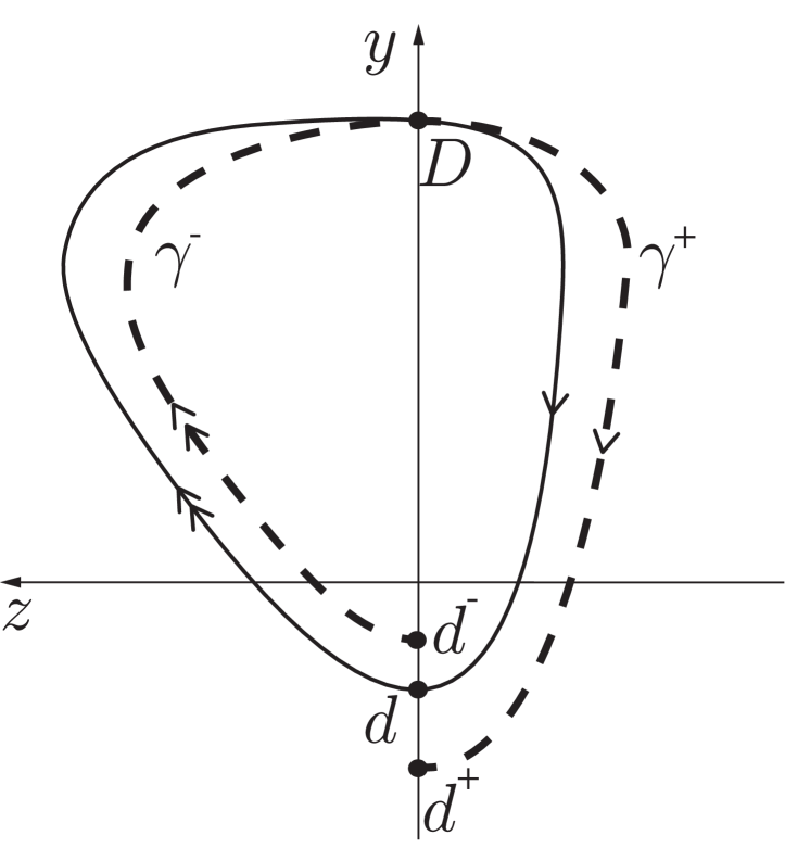
(a)

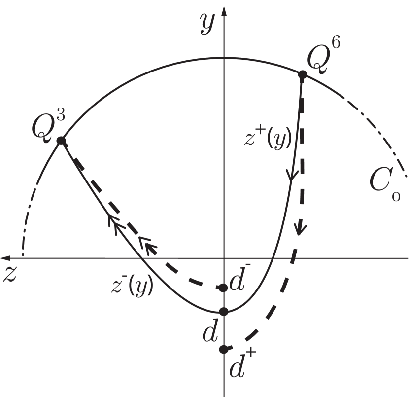
(b)

Figure 8: Perturbation of the Hamiltonian solutions for $\alpha-\xi$ small. In 8(a): closed orbit with $0<H<1$. In 8(b): heteroclinic connection for $H=1$.

We Taylor expand (37) around $\alpha=\xi$:

$$\Delta(\alpha)=(\alpha-\xi)\Delta_{\alpha}(h)+{\Or((\alpha-\xi)^{2}),}$$ (38)

with the quantity $\Delta_{\alpha}(h)$ defined as:

$$\Delta_{\alpha}(h) =\int_{T_{h}^{-}}^{T_{h}^{+}}\nabla H(h)\cdot\frac{\partial f_{0}}{\partial\alpha}(y,z;\xi)\,\rmd t$$ (39)

$$=\int_{T_{h}^{-},}^{T_{h}^{+}}\xi\rme^{-\xi y}z(\rme^{z}-1)\,\rmd t.$$

In (39) we have denoted with $(y,z)(t)$ the solution of (12) for $H=h$ and $\alpha=\xi$. The times $T_{h}^{\pm}=T_{h}^{\pm}(\xi)$ are the forward and backwards times from $D$ to $d$. The integrand of (39) is always positive for $z\neq 0$ and therefore $\Delta_{\alpha}(h)$ is positive for any $h\in(0,1)$. We conclude from (38) that the forward flow $\gamma^{+}(t)$ spirals outwards for $\alpha>\xi$ while it spirals inwards for $\alpha<\xi$, in agreement with Figure 6.
We now extend the analysis above to the case of $H=1$. In this case the points $d^{+}$ and $d^{-}$ are the intersections of $W^{c,u}$ and $W^{c,s}$ with the $y$-axis respectively, see Figure 8(b). From the analysis above we know that $W^{c,s}$ and $W^{c,u}$ depend smoothly on $\alpha$.

Lemma 5.5

For $\alpha=\xi$ there is a unique heteroclinic connection between $Q^{3}$ and $Q^{6}$ on $C_{0}$. This connection is through the manifolds $W^{c,s}$ and $W^{c,u}$ and it corresponds to the set $H=1$ in (13b). This set can be written as the union of two graphs $z=z^{\pm}(y)$ (see Figure 8(b)) with $y\geq-1/\xi$ so that $z^{-}(y)\,\,\left(z^{+}(y)\text{ resp.}\right)$ approaches $Q^{3}\,\,\left(Q^{6}\right)$ as $z^{-}=\Or(y)\,\,\left(z^{+}=\Or\left(\ln(y)\right)\,\right)$ for $y\to\infty$.

• We rewrite the trajectory $H=1$ as the graphs $z=z^{\pm}(y)$ for $y\geq-1/\xi$. The behaviour in forward time follows by considering the point $p_{1,\text{in}}$ in condition (25) and blowing it down to the original variables $(y,z)$. Similarly for the behaviour in backwards time by considering $p_{3,\text{out}}$ in condition (36). $\Box$

Figure 6(b) follows from Lemma 5.5. When $\alpha=\xi$ the manifolds $W^{c,s}$ and $W^{c,u}$ cross the $y$-axis in the point $d:=(y,z)=(-1/\xi,0)$. We define the distance function $\Delta(\alpha)$ as in (37), we Taylor expand it around $\alpha=\xi$ as in (38) and we define $\Delta_{\alpha}(1)$ as in (39). Since the integrand of (39) is positive for $H=1$ we just need to show that the improper integral (39) exists. From the reduced problem (11) we observe that $\dot{y}=\rme^{z}-1$, thus we rewrite (39) with respect to $y$ as:

$$\Delta_{\alpha}(1)=\int_{-1/\xi}^{+\infty}\xi\rme^{-\xi y}z^{-}(y)\,\rmd y-\int_{-1/\xi}^{+\infty}\xi\rme^{-\xi y}z^{+}(y)\,\rmd y.$$ (40)

Recall from Lemma 5.5 that $z^{-}(y)$ is asymptotically linear in $y$ for $y\to\infty$, while $z^{+}(y)$ decreases logarithmically with respect to $y$. The expression (40) therefore exists because of the exponential decay of the factor $\exp({-\xi y})$ and furthermore it is positive. We remark that $\Delta_{\alpha}(h)$ in (39) converges to $\Delta_{\alpha}(1)$ for $h\to 1$, since the orbit segment on $C_{0,\infty}$ does not give any contribution to (40).

Now we finish the proof of Proposition 5.2 by considering $\alpha$ as in (21). When $\alpha<\xi$ the set $W^{c,u}$ contracts to the origin, because $\Delta(\alpha)<0$ in (38). Furthermore the set $W^{c,s}$ is backwards asymptotic to $Q^{7}$ and acts as a separator between the basin of attraction of the origin and the basin of attraction of $Q^{1}$. A similar argument covers the case $\alpha>\xi$. This concludes the proof of Proposition 5.2 and justifies Figures 6(a) and 6(c). Therefore no periodic orbit exists on $C_{0}$ for $\alpha>\xi$ and $\varepsilon=0$.

6 Analysis of the perturbed problem for $\varepsilon>0$

Consider the original problem (1) and $0<\mu<1$ small but fixed. Then the compact manifold:

$$S_{0}=\{(x,y,z)\in C_{0}\lvert\quad 0\leq H(y,z)\leq 1-\mu\},$$ (41)

is normally hyperbolic for $\varepsilon=0$. Therefore Fenichel’s theory guarantees that for $\varepsilon$ sufficiently small there exists a locally invariant manifold $S_{\varepsilon}$ that is $\Or(\varepsilon)$-close to $S_{0}$ and is diffeomorphic to it. Moreover the flow on $S_{\varepsilon}$ converges to the flow of the reduced problem (11) for $\varepsilon\to 0$. A computation shows that $S_{\varepsilon}$ at first order is:

$$z=-(x+\xi y)+\varepsilon\xi\rme^{-2(x+\xi y)}\left(\alpha(x+\xi y)+\xi(y+1)-\xi\rme^{x+\xi y}\right)+\Or(\varepsilon^{2}),$$

hence we have the following vector field $f_{\varepsilon}(y,z;\alpha,\varepsilon)$ on $S_{\varepsilon}$:

$$f_{\varepsilon}(y,z;\alpha,\varepsilon):=\begin{cases}\dot{y}&=\rme^{z}-1-\varepsilon\xi\chi\rme^{2z}+\Or(\varepsilon^{2}),\\ \dot{z}&=\chi-\varepsilon\xi\chi\rme^{2z}(\alpha z-\xi y+\alpha-\xi+1)+\Or(\varepsilon^{2}),\end{cases}$$ (42)

with $\chi(y,z)=\alpha z\rme^{z}-\xi y\rme^{z}-\xi\rme^{z}+\xi$.

Proposition 6.1

Consider the compact manifold $S_{0}$ defined in (41). Then $S_{0}$ perturbs to a locally invariant slow manifold $S_{\varepsilon}$ for $0<\varepsilon\ll 1$. On $S_{\varepsilon}$ the origin of (42) undergoes a supercritical Hopf bifurcation for:

$$\alpha=\alpha_{H}:=\xi-\varepsilon\xi^{2}+\Or(\varepsilon^{2}),$$ (43)

with a negative first Lyapunov coefficient:

$$a=-\frac{1}{8}\varepsilon\xi^{3}(1+\xi)+\Or(\varepsilon^{2})<0.$$ (44)

Therefore for $\alpha\in\left(\alpha_{H},\alpha_{H}+c(\mu)\varepsilon\right)$ with $c(\mu)$ sufficiently small, there exists a family of locally unique attracting limit cycles with amplitude of order $\Or\left(\sqrt{-(\alpha-\alpha_{H})/a}\right)$.

The proof of Proposition 6.1 follows from straightforward computations. We remark that since (44) is proportional to $\varepsilon$, it follows that the results of Proposition 6.1 are valid only for a very small interval of $\alpha$ around $\alpha_{H}$. We use the analysis of section 5.3 to extend the small limit cycles of Proposition 6.1 into larger ones.

Proposition 6.2

Consider the slow manifold $S_{\varepsilon}$ of Proposition 6.1. On $S_{\varepsilon}$ there exists a family of closed periodic orbits for

$$\alpha=\alpha_{M}(h):=\xi-\varepsilon\frac{\Delta_{\varepsilon}(h)}{\Delta_{\alpha}(h)}+\Or(\varepsilon^{2}),$$ (45)

where $h\in[c_{1}(\mu),1-c_{2}(\mu)]$ with $(c_{1},c_{2})(\mu)$ small. The quantity $\mathit{\Delta}_{\varepsilon}(h)$ is defined as:

$$\Delta_{\varepsilon}(h)=\int_{T_{h}^{-}}^{T_{h}^{+}}\nabla H(h)\cdot\frac{\partial f_{\varepsilon}}{\partial\varepsilon}(y,z;\xi,0)\,\rmd t,$$ (46)

while $\Delta_{\alpha}(h)>0$ was defined in (39).

• By Fenichel’s theorem we know that the flow on $S_{\varepsilon}$ converges to the flow of the reduced problem (11) for $\varepsilon\to 0$. Therefore we can define the distance function $\Delta(\alpha,\varepsilon)$ similarly to (37) whose Taylor expansion around $\alpha=\xi$ and $\varepsilon=0$ is:

  $$\Delta(\alpha,\varepsilon)=(\alpha-\xi)\Delta_{\alpha}(h)+\varepsilon\Delta_{\varepsilon}(h)+\Or((\alpha-\xi+\varepsilon)^{2}),$$ (47)

  with $\Delta_{\alpha}(h)$ and $\Delta_{\varepsilon}(h)$ defined in (39) and (46) respectively. The integrand of $\Delta_{\alpha}(h)$ is strictly positive for all $h\in(0,1)$, therefore we can apply the implicit function theorem to (47) for $\Delta(\alpha,\varepsilon)=0$ and obtain the result (45). $\Box$

In Figure 9 we show a numerical computation of the leading order coefficient in (45) for an interval of energies $H=h\in(0,0.6]$. No saddle-node bifurcations occur in this interval and hence the periodic orbits are all asymptotically stable. We expect a similar behaviour for larger values of $h$ but we did not manage to compute this due to the intrinsic slow-fast structure of the reduced problem. It might be possible to study the term $\Delta_{\varepsilon}(h)/\Delta_{\alpha}(h)$ analytically by using the results of Lemma 5.5 but the expressions are lengthy and we did not find an easy way.
The analysis above can only explain the limit cycles that appear for $\alpha-\xi=\Or(\varepsilon)$ and it does not justify the limit cycles of Figure 1 that appear for larger values of $\alpha-\xi$. For this reason we proceed to study the full problem (1) at infinity, introducing its compactification through the Poincaré sphere.

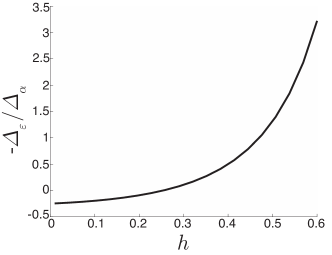
Figure 9: Plot of the leading order coefficient in (45) for $\xi=0.5$ and $h\in(0,0.6]$.

7 Statement of the main result

In this section we find a connection at infinity between the points $Q^{1}$ and $Q^{6}$ (recall Proposition 5.1) that will establish a return mechanism to $C_{0}$ of the unbounded solutions of (4) when $\varepsilon=0$ and $\alpha>\xi$. This mechanism will be the foundation for the existence of limit cycles when $0<\varepsilon\ll 1$ and $\alpha-\xi\geq c>0$.
Similar to section 5, we introduce a four-dimensional Poincaré sphere $\mathcal{S}^{3,+}$:

$$\mathcal{S}^{3,+}:=\left\{(X,Y,Z,W)\in\mathbb{R}^{4}\bigr{|}\quad X^{2}+Y^{2}+Z^{2}+W^{2}=1,\quad W\geq 0\right\}.$$ (48)

The fast problem (4) is interpreted as a directional chart ${K}_{2}$ on $\mathcal{S}^{3,+}$ defined for $W=1$:

$${K}_{2}:=\mathcal{S}^{3,+}\cap\{W=1\},\quad x_{2}=\frac{X}{W},y_{2}=\frac{Y}{W},z_{2}=\frac{Z}{W},$$

therefore the vector field in chart $K_{2}$ is obtained by introducing the subscript in (4):

$$\dot{x}_{2} =-\varepsilon\rme^{z_{2}}(x_{2}+(1+\alpha)z_{2}),$$ (49)

$$\dot{y}_{2} =\varepsilon\left(\rme^{z_{2}}-1\right),$$

$$\dot{z}_{2} =-\rme^{-z_{2}}\left(y_{2}+\frac{x_{2}+z_{2}}{\xi}\right).$$

The points at infinity in ${K}_{2}$ correspond to $W=0$ which is a sphere ${S}^{2}$. We introduce the two directional charts:

$${K}_{3}:=\mathcal{S}^{3,+}\cap\{Z=1\},\quad x_{3}=\frac{X}{Z},y_{3}=\frac{Y}{Z},w_{3}=\frac{W}{Z},$$ (50a)

$${K}_{1}:=\mathcal{S}^{3,+}\cap\{Y=1\},\quad x_{1}=\frac{X}{Y},z_{1}=\frac{Z}{Y},w_{1}=\frac{W}{Y}.$$ (50b)

We have the following transformations between the charts:

$${K}_{23}:\quad w_{3}=z_{2}^{-1},\quad\,x_{3}=x_{2}z_{2}^{-1},\quad y_{3}=y_{2}z_{2}^{-1},$$ (51a)

$${K}_{21}:\quad w_{1}=y_{2}^{-1},\quad\,x_{1}=x_{2}y_{2}^{-1},\quad z_{1}=z_{2}y_{2}^{-1},$$ (51b)

$${K}_{31}:\quad w_{1}=w_{3}y_{3}^{-1},\,x_{1}=x_{3}y_{3}^{-1},\quad z_{1}=y_{3}^{-1},$$ (51c)

that are defined for $z_{2}>0$, $y_{2}>0$ and $y_{3}>0$ respectively. The inverse transformations are defined similarly. The three points $Q^{1},Q^{3}\in K_{3}$ and $Q^{6}\in K_{1}$:

$$Q^{1}:=\quad(x_{3},y_{3},w_{3})=(-1,0,0),$$ (52a)

$$Q^{3}:=\quad(x_{3},y_{3},w_{3})=\left(-1-\alpha,\frac{\alpha}{\xi},0\right),$$ (52b)

$$Q^{6}:=\quad(x_{1},z_{1},w_{1})=\left(-\xi,0,0\right),$$ (52c)

introduced in Proposition 5.1 and the three points $Q^{2},Q^{4}\in K_{3}$ and $Q^{5}\in K_{1}$:

$$Q^{2}:=\quad(x_{3},y_{3},w_{3})=(-1-\alpha,0,0),$$ (53a)

$$Q^{4}:=\quad(x_{3},y_{3},w_{3})=\left(-1-\alpha,\frac{2\alpha}{\xi},0\right),$$ (53b)

$$Q^{5}:=\quad(x_{1},z_{1},w_{1})=\left(-\frac{\xi}{2\alpha}(1+\alpha),\frac{\xi}{2\alpha}(1-\alpha),0\right),$$ (53c)

are going to play a role in the following, together with the lines:

$$L_{0} :=\quad\left\{(x_{3},y_{3},w_{3})\lvert\quad x_{3}+1+\alpha=0,\,\,w_{3}=0\right\},$$ (54a)

$$C_{0,\infty} :=\quad\left\{(x_{3},y_{3},w_{3})\lvert\quad x_{3}+\xi y_{3}+1=0,\,\,w_{3}=0\right\}.$$ (54b)

Notice that the line $L_{0}$ corresponds to the intersection of the family of nullclines (10) with infinity through $K_{23}$. We construct the following singular cycle:

• Let $\Gamma_{0}$ be the closed orbit consisting of the points $Q^{1,2,4,5,6}$ and of the union of the following sets:

  • $\gamma^{1,2}$ connecting $Q^{1}$ with $Q^{2}$. In chart ${K}_{3}$ the segment $\gamma^{1,2}$ is:

    $$\gamma^{1,2}:=\{(x_{3},y_{3},w_{3})\in{K}_{3}\lvert\quad x_{3}\in(-1-\alpha,-1),y_{3}=0,w_{3}=0\}.$$ (55)

  • $\gamma^{2,4}$ connecting $Q^{2}$ with $Q^{4}$ along $L_{0}$. In chart ${K}_{3}$ the segment $\gamma^{2,4}$ is:

    $$\gamma^{2,4}:=\left\{(x_{3},y_{3},w_{3})\in{K}_{3}\lvert\quad x_{3}=-1-\alpha,y_{3}\in\left(0,\frac{2\alpha}{\xi}\right),w_{3}=0\right\}.$$ (56)

  • $\gamma^{4,5}$ connecting $Q^{4}$ with $Q^{5}$. This segment is a fast fiber of (6) and in chart ${K}_{1}$ the segment $\gamma^{4,5}$ is:

    $$\gamma^{4,5}:=\left\{(x_{1},z_{1},w_{1})\in{K}_{1}\lvert\quad x_{1}=-\frac{\xi}{2\alpha}(1+\alpha),z_{1}\in\left(\frac{\xi}{2\alpha}(1-\alpha),\frac{\xi}{2\alpha}\right),w_{1}=0\right\}.$$ (57)

  • $\gamma^{5,6}$ connecting $Q^{5}$ with $Q^{6}$ on $C_{0,\infty}$. In chart ${K}_{1}$ the segment $\gamma^{5,6}$ is:

    $$\gamma^{5,6}:=\left\{(x_{1},z_{1},w_{1})\in{K}_{1}\lvert\quad x_{1}=-\xi-z_{1},z_{1}\in\left(0,\frac{\xi}{2\alpha}(1-\alpha)\right),w_{1}=0\right\}.$$ (58)

  • $W^{c,u}$ connecting $Q^{6}$ with $Q^{1}$ on the critical manifold $C_{0}$.

In section 8 we identify $\Gamma_{0}$ using repeatedly the blow-up method on system (49). Figure 10 shows $\Gamma_{0}$ and its different segments: 10(a) displays the complete cycle while 10(b) and 10(c) illustrate the portions of $\Gamma_{0}$ that are visible in the charts ${K}_{3}$ and ${K}_{1}$ respectively.

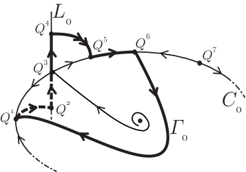
(a)

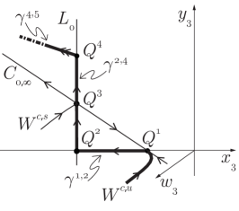
(b)

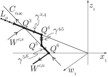
(c)

Figure 10: Schematisation of $\Gamma_{0}$ in 10(a). In chart $K_{3}$ 10(b) we see the segments $\gamma^{1,2},\gamma^{2,4}$ and partially $\gamma^{4,5}$. In chart $K_{1}$ 10(c) we see $\gamma^{4,5},\gamma^{5,6}$ and partially $\gamma^{2,4}$.

$\Gamma_{0}$ plays an important role in our main result, since we conjecture it to be the candidate singular cycle:

Conjecture 7.1

Fix $\alpha>\xi$. Then for $0<\varepsilon\ll 1$ there exists an attracting limit cycle $\Gamma_{\varepsilon}$ that converges to the singular cycle $\Gamma_{0}$ for $\varepsilon\to 0$.

A rigorous proof of Conjecture 7.1 requires an analysis both for $\varepsilon=0$ and $0<\varepsilon\ll 1$. In section 9 we outline a procedure to prove the conjecture and we leave the full details of the proof to a future manuscript.

Remark 7

Here we collect the results of sections 6 and 7. When $\varepsilon=0$ and $\alpha=\xi$ then there exists a family of periodic solutions on $\mathcal{S}^{3,+}$, corresponding to the Hamiltonian orbits with $H\in(0,1)$. For $\alpha>\xi$ only the cycle $\Gamma_{0}$ persists.
When $0<\varepsilon\ll 1$ and $\alpha-\xi=\Or(\varepsilon)$ there exists a limit cycle resembling the bounded Hamiltonian orbits. For larger values of $\alpha-\xi$ we conjecture that the limit cycle tends to $\Gamma_{0}$. Figure 11 shows the conjectured bifurcation diagram of the periodic orbits.

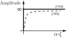
Figure 11: Conjectured bifurcation diagram of the limit cycles for $\varepsilon\ll 1$.

Figure 13 shows some numerical simulations supporting Conjecture 7.1: 12(a) illustrates the limit cycles $\Gamma_{\varepsilon}$ for three different values of $\varepsilon\in\{10^{-8},10^{-4},10^{-2}\}$ with $\alpha=0.9$ and $\xi=0.5$ while 12(b) and 13(a) show the portions of $\Gamma_{\varepsilon}$ that appear in the charts $K_{3}$ and $K_{1}$ respectively. The amplitudes of the orbits increase for decreasing values of the parameter $\varepsilon$ and both the plane $C_{0}$ and the line $L_{0}$ play an important role. Close to the origin the dynamics evolves on $C_{0}$ while sufficiently far from the origin $L_{0}$ becomes relevant. Indeed in Figure 12(b) we see that the solutions contract to $L_{0}$ following $\gamma^{1,2}$ and then they evolve following $\gamma^{2,4}$. When the trajectories are close to $Q^{4}$ they follow $\gamma^{4,5}$ and contract again towards $C_{0}$ along a direction that tends to the fast fiber for $\varepsilon\to 0$, as we can see in Figure 13(a).

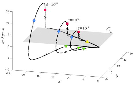
(a)

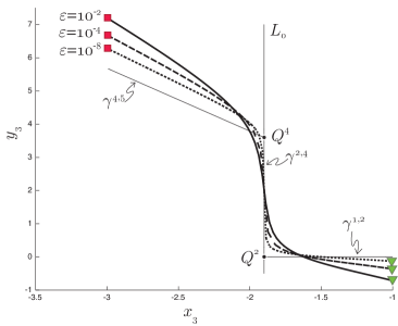
(b)

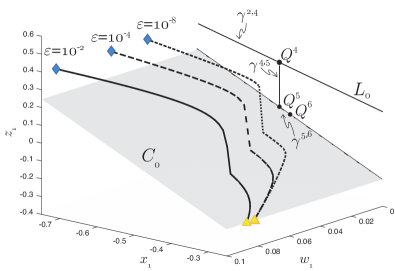
(a)

Figure 13: Figure 12(a): numerical simulation of (1) for $\varepsilon\in\{10^{-8},10^{-4},10^{-2}\}$, $\alpha=0.9$ and $\xi=0.5$. In 12(b): portion of $\Gamma_{\varepsilon}$ visible in chart $K_{3}$, i.e. between the green lower triangle and the red square. In 13(a): portion of $\Gamma_{\varepsilon}$ visible in $K_{1}$, i.e. between the blue diamond and the yellow upper triangle. We remark that the portion between the blue triangle and the red square is visible both in $K_{3}$ and $K_{1}$ since the two charts overlap for $y_{3}>0$ or $z_{1}>0$. Colours are available in the online version.

8 Identification of the segments of $\Gamma_{0}$ at infinity

In this section we focus on the identification of the segments of $\Gamma_{0}$ (55)–(58). We are especially interested in revealing the line $L_{0}$ and the segments that interact with it. In 8.1 we study the dynamics along chart $K_{3}$ and then in 8.2 we consider chart $K_{1}$. More details are available in [Bossolini2015a].

8.1 Chart ${K}_{3}$

We obtain the vector field in chart ${K}_{3}$ by inserting condition (50a) into the fast problem (49). This vector field is de-singularized at $w_{3}=0$ by division of $\rme^{1/w_{3}}$. For the sake of readability we drop the subscripts:

$$\dot{w} =w\rme^{-\frac{2}{w}}\left(y+\frac{x+1}{\xi}\right),$$ (59)

$$\dot{x} =-\varepsilon(x+1+\alpha)+x\rme^{-\frac{2}{w}}\left(y+\frac{x+1}{\xi}\right),$$

$$\dot{y} =\varepsilon w(1-\rme^{-\frac{1}{w}})+y\rme^{-\frac{2}{w}}\left(y+\frac{x+1}{\xi}\right),$$

$$\dot{\varepsilon} =0.$$

System (59) is a four-dimensional vector field defined on $\mathbb{R}^{4}$ where we treat $\varepsilon$ as a variable. The set $w=\varepsilon=0$ consists of non-hyperbolic fixed points of (59) and the two lines $C_{0,\infty}$ and $L_{0}$ (54) are contained within this set. Since we consider a regime of $w$ sufficiently small, we approximate $1-\rme^{-1/w}\simeq 1$ in the $y$-equation of (59) to simplify the computations. Qualitatively this has no effects on the results.
We blow-up (59) around $Q^{1}$ in order to extend the hyperbolicity of $C_{0}$ up to infinity. To do so we need to get rid of the exponential terms. We deal with it by introducing a new variable $q$:

$$q=\rme^{-\frac{2}{w}},$$ (60)

so that the extended system contains only algebraic terms in its variables [Kristiansen2015a]. Indeed by differentiating (60) with respect to time we obtain:

$$\dot{q} =2w^{-2}\dot{w}\rme^{-\frac{2}{w}},$$ (61)

$$=2w^{-1}q\left(y+\frac{x+1}{\xi}\right),$$

where we have used (59) and (60). Inserting (61) into (59) we obtain the five-dimensional vector field:

$$\dot{w} =w^{2}q\left(y+\frac{x+1}{\xi}\right),$$ (62)

$$\dot{x} =-\varepsilon w(x+1+\alpha)+xqw\left(y+\frac{x+1}{\xi}\right),$$

$$\dot{y} =\varepsilon w^{2}+yqw\left(y+\frac{x+1}{\xi}\right),$$

$$\dot{q} =2q^{2}\left(y+\frac{x+1}{\xi}\right),$$

$$\dot{\varepsilon} =0.$$

after multiplying the right hand side by $w$. The evolution of $q$ in (62) is slaved by $w$ through (60). However, this dependence is not explicit and we will refer to it only when needed. We refer to [Kristiansen2015a] for further details on this approach. System (62) has a 3-dimensional space of non-hyperbolic fixed points for $\varepsilon=q=0$, since each point has a quintuple zero eigenvalue. To overcome the degeneracy we introduce the blow-up map:

$$\quad q=\bar{r}\bar{q},\quad\varepsilon=\bar{r}\bar{\epsilon},$$ (63)

with $(\bar{q},\bar{\epsilon})\in S^{1}$ and $\bar{r}\geq 0$ while the variables $(w,x,y)\in\mathbb{R}^{3}$ in (62) are kept unchanged. We remark that the quantity $\varepsilon$ in (63) is a constant, hence the blown-up space is foliated by invariant hyperbolas. We study the two local charts:

$$\mathcal{K}_{1}:\quad q=r_{1},\qquad\varepsilon=r_{1}\epsilon_{1},$$ (64a)

$$\mathcal{K}_{2}:\quad q=r_{2}q_{2},\qquad\varepsilon=r_{2}.$$ (64b)

Notice that $q_{2}=\Or(1)$ in chart $\mathcal{K}_{2}$ corresponds to $w=\Or(\ln^{-1}\varepsilon^{-1})$ or $z_{2}=\Or(\ln\varepsilon^{-1})$ through (60). This is the relevant regime for the naïve identification of $L_{0}$ as in (9).

Chart $\mathcal{K}_{1}$

To simplify the analysis we place the $x$-axis of (62) on $C_{0}$ by introducing the new coordinate $\tilde{x}=x+\xi y+1$ so that $Q^{1}$ is now in the origin of chart ${K}_{3}$. We insert (64a) into (62) and divide out a common factor of $r_{1}$ to obtain the de-singularized system in chart $\mathcal{K}_{1}$. This system is independent of $r_{1}$ therefore we restrict the analysis to the remaining four variables $(w,\tilde{x},y,\epsilon_{1})$ and we drop the subscript. The origin of the reduced system is still degenerate with all zero eigenvalues. To overcome the degeneracy we introduce the following blow-up of $C_{0,\infty}$:

$$w=\bar{r}\bar{w},\quad\tilde{x}=\bar{r}\bar{\tilde{x}},\quad\epsilon=\bar{r}\bar{\epsilon},$$

where $(\bar{w},\bar{\tilde{x}},\bar{\epsilon})\in{S}^{2}$ and $\bar{r}\geq 0$ small, while the variable $y\in\mathbb{R}$ is kept unchanged. We study charts $\mathtt{K}_{1}$ and $\mathtt{K}_{2}$ that are defined for $\bar{w}=1$ and $\bar{\epsilon}=1$ respectively.
Chart $\mathtt{K}_{1}$ has an attracting 3-dimensional center manifold $M_{1}$ in the origin. This manifold is the extension of the slow-manifold $S_{\varepsilon}$ (see Proposition 6.1) into chart $\mathtt{K}_{1}$ when $\varepsilon=\text{const.}$ and $q=\rme^{-2/w}$. Thus we can extend the hyperbolicity of $C_{0}$ up to $C_{0,\infty}$ for $\bar{\epsilon}=0$ and recover the contraction to $Q^{1}$ of Figure 6(c). We follow the unique unstable direction of $Q^{1}$ that sits on the sphere $\bar{r}=0$. This direction exits chart $\mathtt{K}_{1}$ for $\bar{\epsilon}$ large and contracts to the origin of chart $\mathtt{K}_{2}$ along the invariant plane $\bar{r}=0$. Using hyperbolic methods we follow the unique 1-dimensional unstable manifold $\gamma_{2}^{1}$ departing from the origin of chart $\mathtt{K}_{2}$ into chart $\mathcal{K}_{2}$, where it enters with $q_{2}$ small.

Chart $\mathcal{K}_{2}$

We substitute (64b) into (62) and divide the right-hand side by $r_{2}$ to obtain the dynamics in chart $\mathcal{K}_{2}$. The system is independent of $r_{2}$ and we restrict the analysis to $(w,x,y,q_{2})$. The unstable manifold $\gamma_{2}^{1}:=\left\{(w,x,y,q_{2})\in\mathcal{K}_{2}\lvert\quad(w,x,y)=(0,-1,0),q_{2}\geq 0\right\}$ contracts towards the fixed point:

$$(w,x,y,q_{2})=(0,-1,0,0).$$ (65)

The point (65) belongs to a plane of non-hyperbolic fixed points with $w=q_{2}=0$ and to overcome the loss of hyperbolicity we introduce the blow-up map (after having dropped the subscript):

$$w=\bar{r}\bar{w},\quad q=\bar{r}\bar{q},$$ (66)

where $(\bar{w},\bar{q})\in{S}^{1}$ and $\bar{r}\geq 0$. We study charts $\hat{\mathtt{K}}_{1}$ and $\hat{\mathtt{K}}_{2}$ that are defined for $\bar{w}=1$ and $\bar{q}=1$ respectively.

Chart $\hat{\mathtt{K}}_{1}$

We insert (66) with $\bar{w}=1$ into the vector field of chart $\mathcal{K}_{2}$ and drop the bar. We divide the system by $r$ to obtain the de-singularized equations:

$$\dot{r} =r^{2}q\left(y+\frac{x+1}{\xi}\right),$$ (67)

$$\dot{x} =-(x+1+\alpha)+xrq\left(y+\frac{x+1}{\xi}\right),$$

$$\dot{y} =r+yrq\left(y+\frac{x+1}{\xi}\right),$$

$$\dot{q} =q^{2}(2-r)\left(y+\frac{x+1}{\xi}\right).$$

In the following important lemma we identify the line $L_{0}$ and the segment $\gamma^{1,2}$:

Lemma 8.1

In chart $\hat{\mathtt{K}}_{1}$ there exists an attracting 3-dimensional center manifold:

$$x=-1-\alpha+\Or(r+q),$$ (68)

whose intersection with the plane $r=q=0$ corresponds to the line $L_{0}$ (54a). The trajectory $\gamma^{1,2}$ defined in (55) connects along a stable fiber the point (65) to $Q^{2}$ (53a).

• (67) has a line of fixed points for $r=q=0,x=-1-\alpha,y\in\mathbb{R}$. This line corresponds to $L_{0}$ through the coordinate changes (64b), (66). The linearized dynamics on $L_{0}$ is hyperbolic only in the $x$-direction and furthermore is stable. Therefore (68) appears for $r,q$ sufficiently small. The point (65) in chart $\hat{\mathtt{K}}_{1}$ becomes:

  $$(r,x,y,q)=(0,-1,0,0),$$ (69)

  hence there is a solution backwards asymptotic to (69) and forward asymptotic to $Q^{2}\in L_{0}$ (recall (53a)) through a stable fiber. This connection corresponds to $\gamma^{1,2}$. $\Box$

We insert (68) into (67) to obtain the dynamics on the center manifold. The resulting vector field has a line of non-hyperbolic fixed points, corresponding to $L_{0}$, for $r=q=0$ since each point has a triple zero eigenvalue. We gain hyperbolicity of this line by introducing the blow-up map:

$$r=\rho\sigma,\quad q=\rho,$$ (70)

where $\rho\geq 0,\sigma\geq 0$. In chart (70) the point $Q^{2}$ (53a) is blown-up to the $\sigma$-axis $\{y=\rho=0,\sigma\geq 0\}$. Similarly $Q^{4}$ (53b) corresponds to the line $\{y=2\alpha/\xi,\rho=0,\sigma\geq 0\}$. We divide the vector field of chart (70) by the common divisor $\rho$ and obtain:

$$\dot{\sigma} =\sigma(-2+\rho\sigma+\rho^{2})\left(y-\frac{\alpha}{\xi}\right)\left(1+\Or\left(\rho\right)\right),$$ (71)

$$\dot{y} =\sigma+y\rho\sigma\left(y-\frac{\alpha}{\xi}\right)\left(1+\Or\left(\rho\right)\right),$$

$$\dot{\rho} =\rho(2-\rho\sigma)\left(y-\frac{\alpha}{\xi}\right)\left(1+\Or\left(\rho\right)\right).$$

Following equations (65) and $\gamma_{2}^{1}$ we enter chart (70) with $\sigma=0$ and $y=0$. Subsequently, by following $\gamma^{1,2}$ we have $\rho=0$. In the following we describe the dynamics within $L_{0}$ and identify $\gamma^{2,4}$ as a heteroclinic orbit.

Lemma 8.2

System (71) has two invariant planes for $\rho=0$ and $\sigma=0$. Their intersection $\rho=\sigma=0$ is a line of fixed points. We have:

• The origin $(\sigma,y,\rho)=(0,0,0)$ has a strong stable manifold:

  $$W^{s}(0,0,0):=\left\{(\sigma,y,\rho)\in\mathbb{R}^{2}\times\mathbb{R}_{+}\lvert\quad\sigma=0,y=0,\rho\geq 0\right\}.$$ (72)

• There exists a heteroclinic connection:

  $$\gamma^{2,4}=\left\{(\sigma,y,\rho)\in\mathbb{R}^{2}\times\mathbb{R}_{+}\lvert\quad\sigma=2\frac{\alpha}{\xi}y-y^{2},y\in(0,2\alpha/\xi),\rho=0\right\}.$$ (73)

  joining $(\sigma,y,\rho)=(0,0,0)$ backwards in time with $(\sigma,y,\rho)=(0,2\alpha/\xi,0)$ forward in time.

• The point $(\sigma,y,\rho)=(0,2\alpha/\xi,0)$ has a strong unstable manifold:

  $$W^{u}(0,2\alpha/\xi,0):=\left\{(\sigma,y,\rho)\in\mathbb{R}^{2}\times\mathbb{R}_{+}\lvert\quad\sigma=0,y=2\alpha/\xi,\rho\geq 0\right\}.$$ (74)

The results of Lemma 8.2 are summarized in Figure 14.

Remark 8

Upon blowing down, the expression in (73) gives $\gamma^{2,4}$ in (56). We use the same symbol in (73) and (56) for simplicity.

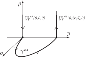
Figure 14: Dynamics in chart $\hat{\mathtt{K}}_{1}$. The plane $\rho=0$ corresponds to the blown-up line $L_{0}$. Here the singular dynamics contracts to $L_{0}$ and then is expelled from it.

• On the invariant plane $\sigma=0$ we have the following dynamics:

  $$\dot{y} =0,$$ (75)

  $$\dot{\rho} =2\rho\left(y-\frac{\alpha}{\xi}\right)\left(1+\Or\left(\rho\right)\right).$$

  This plane is foliated with invariant lines in the $y$-direction. The solution of (75) with $y=0$ is (72) and contracts towards the invariant plane $\rho=0$. Hence this trajectory acts as a strong stable manifold. We substitute $\rho=0$ into (71) and after dividing by $\sigma$ we obtain the explicit solution (73) given the initial condition in the origin. This solution is forward asymptotic to $(\sigma,y,\rho)=(0,2\alpha/\xi,0)$. Eventually $\rho$ expands on the strong unstable manifold (74), that is the solution of (75) with $y=2\alpha/\xi$. $\Box$

Using hyperbolic methods we follow the unstable manifold $W^{u}(0,2\alpha/\xi,0)$ into chart $\hat{\mathtt{K}}_{2}$ where it contracts towards the origin along the invariant plane $\bar{r}=0$. We continue this trajectory by following the unstable manifold of the origin on the plane $\bar{w}=0$. We continue this manifold into chart $\mathcal{K}_{1}$, since eventually chart $\mathcal{K}_{2}$ is no longer suited to describe this trajectory. Here the variable $\epsilon$ decreases exponentially and for $\epsilon=w=0$ we obtain a layer problem. Therefore from $Q^{4}$ we follow after de-singularization a fast fiber $\gamma^{4,5}$ that corresponds to the solution of this layer problem and that contracts to the point $Q^{5}$ on $C_{0}$. Since $Q^{5}$ may not be visible in chart ${K}_{3}$, we compute its coordinates in chart ${K}_{1}$.

8.2 Chart ${K}_{1}$

We insert (51b) into the fast problem (49) and divide by $\rme^{z_{1}/w_{1}}$ to obtain the de-singularized vector field in chart ${K}_{1}$. We drop the subscript henceforth for the sake of readability:

$$\dot{w} =-\varepsilon w^{2}(1-\rme^{-z/w}),$$ (76)

$$\dot{x} =-\varepsilon\left(x+(1+\alpha)z\right)-\varepsilon xw(1-\rme^{-z/w}),$$

$$\dot{z} =-\rme^{-2z/w}\left(1+\frac{x+z}{\xi}\right)-\varepsilon zw(1-\rme^{-z/w}).$$

In chart ${K}_{1}$ the layer problem is obtained by requiring $\varepsilon=0$ in (76). Hence the dynamics on the layer problem is only in the $z$-direction and the fibers are all vertical. In particular the fiber $\gamma^{4,5}$ is written as in (57) since it departs from $K_{31}(Q^{4})$. It follows that $\gamma^{4,5}$ is forward asymptotic to the point $Q^{5}$ defined in (53c). The point $Q^{5}$ is connected to $Q^{6}$ through the segment $\gamma^{5,6}$, according to the analysis of the reduced problem of section 5. From the point $Q^{6}$ the solution is connected to the point $Q^{1}$ through the manifold $W^{c,u}$. This closes the singular cycle $\Gamma_{0}$.
Figure 10(c) illustrates the dynamics in chart ${K}_{1}$. We remark that the change of coordinates from chart ${K}_{3}$ to chart ${K}_{1}$ is defined for $z_{1}>0$ and therefore when $\alpha>1$ the point $Q^{5}$ is visible only in chart ${K}_{1}$.

9 Outline of a proof

To prove Conjecture 7.1 we would have to consider a section $\Lambda_{1}:=\{w_{1}=\delta\}$ transverse to $W^{c,u}$ where $\delta>0$ is small but fixed. Using the blow-up in chart ${K}_{3}$ we can track a full neighbourhood $N\subset\Lambda_{1}$ of $\Lambda_{1}\cap W^{c,u}$ using Proposition 5.2, $\gamma^{1,2},\gamma^{2,4},\gamma^{4,5},\gamma^{5,6}$ and $W^{c,u}$ respectively, to obtain a return map $P_{1}:N\to N$ for $\varepsilon$ sufficiently small. For $\varepsilon=0$ the forward flow of $N$ contracts to the point $Q^{1}$. This would provide the desired contraction of $P_{1}$ and establish, by the contraction mapping theorem, the existence of the limit cycle $\Gamma_{\varepsilon}$ satisfying $\Gamma_{\varepsilon}\to\Gamma_{0}$ for $\varepsilon\to 0$.

10 Conclusions

We have considered the one dimensional spring-block model that describes the earthquake faulting phenomenon. We have used geometric singular perturbation theory and the blow-up method to provide a detailed description of the periodicity of the earthquake episodes, in particular we have untangled the increase in amplitude of the cycles for $\varepsilon\to 0$ and their relaxation oscillation structure. We have shown that the limit cycles arise from a degenerate Hopf bifurcation. The degeneracy is due to an underlying Hamiltonian structure that leads to large amplitude oscillations. Using the Poincaré compactification together with the blow-up method, we have described how these limit cycles behave near infinity in the limit of $\varepsilon\to 0$. A full detailed proof of Conjecture 7.1, including the required careful estimation of the contraction, will be the subject of a separate manuscript.
We have observed that the notation of quasi-static slip motion to define the reduced problem (11) is misleading. Indeed the solutions of (11) have an intrinsic slow-fast structure resembling the stick-slip oscillations. Our analysis also shows that the periodic solutions of (1) cannot be investigated by studying the so-called quasi-static slip phase and the stick-slip phase separately, as it is done in [Ruina1983, gu1984a], since the two phases are connected by the non-linear terms of (1). We also suggest suitable coordinate sets and time rescales to deal with the stiffness of (1) during numerical simulations. We hope that a deeper understanding of the structure of the earthquake cycles may be of help to the temporal predictability of the earthquake episodes.
We presuppose that we can apply some of the ideas in this manuscript to the study of the 1-dimensional spring-block model with Dieterich state law. Indeed in this new system the fixed point in the origin behaves like a saddle, the critical manifold loses hyperbolicity like (8) and solutions reach infinity in finite time for $\varepsilon\to 0$. Moreover we think that these ideas can also be used to study the continuum formulation of the Burridge and Knopoff model with Ruina state law, in particular to analyse the self-healing slip pulse solutions [heaton1990a]. Indeed this latter model has the same difficulties of (1) in terms of small parameter and non-linearities of the vector field [Erickson2011]. We remark that the self-healing slip pulse solutions are considered to be related to the energy of an earthquake rupture.

References

References

- [1] \harvarditemBelardinelli \harvardand Belardinelli1996belardinelli1996a Belardinelli M E \harvardand Belardinelli E 1996 Nonlinear Processes in Geophysics 3(3), 143–149.
- [2] \harvarditemBen-Zion2008Ben-zion2008 Ben-Zion Y 2008 Reviews of Geophysics 46(4). RG4006.
- [3] \harvarditemBizzarri2010bizzarri2010a Bizzarri A 2010 Geophysical Research Letters 37(20). L20315.
- [4] \harvarditemBossolini et al.2016Bossolini2015a Bossolini E, Brøns M \harvardand Kristiansen K U 2016 ArXiv e-prints arXiv:1603.02448v1 [math.DS] .
- [5] \harvarditemBurridge \harvardand Knopoff1967Burridge1967 Burridge R \harvardand Knopoff L 1967 Bulletin of the Seismological Society of America 57(3), 341–371.
- [6] \harvarditemCarlson \harvardand Langer1989carlson1989a Carlson J M \harvardand Langer J S 1989 Physical Review A 40(11), 6470–6484.
- [7] \harvarditemCarlson et al.1991carlson1991a Carlson J M, Langer J S, Shaw B E \harvardand Tang C 1991 Physical Review A 44(2), 884–897.
- [8] \harvarditemChicone2006chicone2006a Chicone C 2006 Ordinary differential equations with applications Springer Science+Business Media.
- [9] \harvarditemChow et al.1994Chow94 Chow S N, Li C \harvardand Wang D 1994 Normal Forms and Bifurcation of Planar Vector Fields Cambridge University Press.
- [10] \harvarditemCorless et al.1996corless2014a Corless R M, Gonnet G H, Hare D E G, Jeffrey D J \harvardand Knuth D E 1996 Advances in Computational Mathematics 5(1), 329–359.
- [11] \harvarditemDieterich1972dieterich1972 Dieterich J H 1972 Journal of Geophysical Research 77(20), 3690–3697.
- [12] \harvarditemDieterich1978dieterich1978a Dieterich J H 1978 Pure and Applied Geophysics 116(4-5), 790–806.
- [13] \harvarditemDieterich1979Dieterich1979 Dieterich J H 1979 Journal of Geophysical Research 84(B5), 2161–2168.
- [14] \harvarditemDumortier \harvardand Roussarie1996dumortier1996a Dumortier F \harvardand Roussarie R 1996 Memoirs of the American Mathematical Society 121(577).
- [15] \harvarditemEckhaus1973eckhaus1973a Eckhaus W 1973 Matched asymptotic expansions and singular perturbations North-Holland Publ.
- [16] \harvarditemErickson et al.2008Erickson2008 Erickson B, Birnir B \harvardand Lavallée D 2008 Nonlinear Processes in Geophysics 15(1), 1–12.
- [17] \harvarditemErickson et al.2011Erickson2011 Erickson B, Birnir B \harvardand Lavallée D 2011 Geophysical Journal International 187(1), 178–198.
- [18] \harvarditemFan et al.2014fan2014a Fan Q, Xu C, Niu J, Jiang G \harvardand Liu Y 2014 Journal of Seismology 18(3), 637–649.
- [19] \harvarditemFenichel1974fenichel1974a Fenichel N 1974 Indiana University Mathematics Journal 23(12), 1109–1137.
- [20] \harvarditemFenichel1979Fenichel1979 Fenichel N 1979 Journal of Differential Equations 31(1), 53–98.
- [21] \harvarditemGu et al.1984gu1984a Gu J C, Rice J R, Ruina A L \harvardand Tse S T 1984 Journal of the Mechanics and Physics of Solids 32(3), 167–196.
- [22] \harvarditemGucwa \harvardand Szmolyan2009Gucwa2009783 Gucwa I \harvardand Szmolyan P 2009 Discrete and Continuous Dynamical Systems - Series S 2(4), 783–806.
- [23] \harvarditemHeaton1990heaton1990a Heaton T H 1990 Physics of the Earth and Planetary Interiors 64(1), 1–20.
- [24] \harvarditemJones1995Jones1995 Jones C K R T 1995 in R Johnson, ed., ‘Dynamical Systems’ Vol. 1609 of Lecture Notes in Mathematics Springer Berlin Heidelberg pp. 44–118.
- [25] \harvarditemKaper1999Kaper1999 Kaper T J 1999 in ‘Proceedings of Symposia in Applied Mathematics’ Vol. 56 American Mathematical Society pp. 85–132.
- [26] \harvarditemKristiansen2016Kristiansen2015a Kristiansen K U 2016 ArXiv e-prints arXiv:1603.01821 [math.DS] .
- [27] \harvarditemKrupa \harvardand Szmolyan2001Krupa2001 Krupa M \harvardand Szmolyan P 2001 SIAM Journal on Mathematical Analysis 33(2), 286–314.
- [28] \harvarditemKuehn2014kuehn2014a Kuehn C 2014 Nonlinearity 27(6), 1351–1366.
- [29] \harvarditemKuehn2015Kuehn2015 Kuehn C 2015 Multiple Time Scale Dynamics Vol. 191 of Applied Mathematical Sciences Springer International Publishing.
- [30] \harvarditemLapusta et al.2000lapusta2000a Lapusta N, Rice J R, Ben-Zion Y \harvardand Zheng G T 2000 Journal of Geophysical Research 105(B10), 23765–23789.
- [31] \harvarditemMadariaga1998Madariaga1998 Madariaga R 1998 Complex Heterogeneous Faulting Models. Unpublished notes (Preprint).
- [32] \harvarditemMadariaga \harvardand Cochard1996madariaga1996a Madariaga R \harvardand Cochard A 1996 Proceedings of the National Academy of Sciences of the United States of America 93(9), 3819–3824.
- [33] \harvarditemMarone1998amarone1998a Marone C 1998a Nature 391(6662), 69–72.
- [34] \harvarditemMarone1998bMarone1998 Marone C 1998b Annual Review of Earth and Planetary Sciences 26, 643–696.
- [35] \harvarditemMarone et al.1995Marone1995 Marone C, Vidale J E \harvardand Ellsworth W L 1995 Geophysical Research Letters 22(22), 3095–3098.
- [36] \harvarditemNadeau \harvardand McEvilly1999Nadeau1999 Nadeau R M \harvardand McEvilly T V 1999 Science 285(5428), 718–721.
- [37] \harvarditemNakatani2001Nakatani2001 Nakatani M 2001 Journal of Geophysical Research: Solid Earth 106(B7), 13347–13380.
- [38] \harvarditemPomeau \harvardand Berre2011pomeau2011critical Pomeau Y \harvardand Berre M L 2011 ArXiv e-prints arXiv:1107.3331 [physics.geo-ph] .
- [39] \harvarditemPutelat et al.2008putelat2008a Putelat T, Willis J R \harvardand Dawes J H P 2008 Philosophical Magazine 88(28–29), 3219–3243.
- [40] \harvarditemRanjith \harvardand Rice1999ranjith1999a Ranjith K \harvardand Rice J R 1999 Journal of the Mechanics and Physics of Solids 47(6), 1207–1218.
- [41] \harvarditemRankin et al.2011rankin2011a Rankin J, Desroches M, Krauskopf B \harvardand Lowenberg M 2011 Nonlinear Dynamics 66(4), 681–688.
- [42] \harvarditemRice \harvardand Ruina1983rice1983a Rice J R \harvardand Ruina A L 1983 Journal of Applied Mechanics 50(2), 343–349.
- [43] \harvarditemRice \harvardand Tse1986rice1986a Rice J R \harvardand Tse S T 1986 Journal of Geophysical Research 91(B1), 521–530.
- [44] \harvarditemRuina1983Ruina1983 Ruina A 1983 Journal of Geophysical Research: Solid Earth 88(B12), 10359–10370.
- [45] \harvarditemVidale et al.1994vidale1994a Vidale J E, Ellsworth W L, Cole A \harvardand Marone C 1994 Nature 368(6472), 624–626.
- [46] \harvarditemZechar \harvardand Nadeau2012Zechar2012 Zechar J D \harvardand Nadeau R M 2012 Geophysical Journal International 190(1), 457–462.
- [47]