A Mathematical Model of Foreign Capital Inflow

Abstract

The paper models foreign capital inflow from the developed to the developing countries in a stochastic dynamic programming (SDP) framework. Under some regularity conditions, the existence of the solutions to the SDP problem is proved and they are then obtained by numerical technique because of the non-linearity of the related functions. A number of comparative dynamic analyses explore the impact of parameters of the model on dynamic paths of capital inflow, interest rate in the international loan market and the exchange rate.

JEL Classification: C61, E44, E47, F32, F34, F42, G11

Mathematics Subject Classification: 90C39, 91-08, 91G10, 91G30

Keywords and Phrases: Capital Inflow, Interest Rate Determination, Dynamic Programming Principle, Portfolio Theory, E-M Algorithm, Dynamic Terms of Trade

1 Introduction

The paper develops a simple model of foreign capital inflow in a multi period dynamic programming frame work. Typically capital flows from the developed to the developing countries owing to a higher rate of return in the latter because of scarcity of capital and thus a higher marginal product of capital than in the developed countries which are capital rich with a lower marginal product of capital. The foreign capital supplements the domestic resources of the developing countries for achieving a higher rate of capital formation and hence higher rate of economic growth. Generally developing countries are characterized by consistent current account deficit. This together with a higher interest rate creates a natural condition for flow of capital from the developed to the developing countries. The inflow to the borrowing country helps appreciate the domestic currency followed by rise in asset prices and local goods prices which via favourable fiscal conditions further encourages domestic credit creation. Repayment of loans in the next period has an adverse effect on exchange rate resulting into depreciation of exchange rate. This does not matter as long as inflow is sufficient. The crisis situation occurs particularly when the rate of capital inflow reaches a plateau or the global investors find a new country with even a higher rate of return then the new paradigm looks shop worn; a sudden stop a la Calvo (1998) to capital inflow or a reversal of current account balance leading to asset price contraction, decreased domestic investment and the economy adjusts backwards. In an extreme situation depreciation of domestic currency makes debt servicing difficult which can lead to a foreign exchange crisis or banking crisis or both (see Reinhart and Reinhart, 2008; Reinhart and Rogoff, 2009; Wolf, 2008). The crisis may further get aggravated by bad macroeconomic management on fiscal and monetary fronts. The problem of debt servicing arises because capital inflow to developing countries are typically pegged in hard currency which has been termed as ’original sin’ (Eichengreen and Hausman, 1999; Eichengreen, Hausman and Panizza, 2005).

In a simple two period model the potential of financial crisis emanating from the depreciation of exchange rate at the time of repayment of foreign currency loans was modeled by Marjit, Das and Bardhan (2007). The argument is based on simple text book explanation of terms of trade effect based on trade theoretic argument as in Caves et al 1993; Helpman and Krugman, 1989. When all the producers sell in the international market at a given world price the combined supply reduces the world price though no individual seller or even a country can affect world price. The same argument applies in the context of capital inflow in a two period framework. It is argued that the terms of trade effect may dominate leading to a financial crisis. Basak, Das and Marjit (2012) extended the model by introducing repayment of previous period borrowing. It adds multi period dynamics in the structure for a better understanding of the possibility of crisis. Costinot et al. (2014) has argued for capital control on the basis of dynamic terms of trade in the same spirit as in this paper. The present paper is a formalization of the process of capital inflow in an infinite horizon set up with micro foundations of the choice problem of the agents - borrowers and lenders. The model investigates the effect of an increase in the perception of risk of default of international loan in the lending country, shift in the expectation of the future exchange rate or decreased productivity in the domestic sector in the borrowing country on capital inflow. The issue pertaining to the origin of the financial crisis in the process of inflow is also discussed.

With this short introduction the paper proceeds as follows. Section 2 formulates a model of capital inflow in a two country setup, a borrowing country and a lending country. From the individual optimization exercise we derive equilibria in the two markets, viz. international loan market and the foreign exchange market which are then solved for the interest rate in the international loan market and exchange rate by numerical method. Proofs of the existence of the solutions are given in the Appendices. In section 3, we undertake comparative dynamic exercises of changes in parameter values. The final section concludes.

2 The Model

We consider a two-country model with one borrowing (developing) and another lending (developed) country. The two country framework is an abstraction from the reality where the two countries represent two country groups. The borrowing country group is capital scarce, thus has a higher marginal product of capital and hence a higher domestic interest rates whereas the lending country has lower domestic interest rates as this group is capital rich. Actual borrowing-lending takes place through banks or financial intermediaries, there is no direct lending. A typical bank in the developing country borrows from both the domestic and international markets and lends to domestic production sector while a typical bank in the developed country borrows from domestic sector and lends to both the domestic and international borrowers. The developing country banks have to repay the foreign debt along with the interest rate in the next period denominated in the lending country’s currency, i.e., hard currency. International loan market is assumed to be competitive so that the international loan rate is given to both lending country and borrowing country banks. We do not consider the determination of domestic borrowing or lending rates of interest in the model. It is only the interest rate on foreign borrowing/ lending and the exchange rate that are determined in this model. Each bank in both the developed and the developing countries maximize discounted expected utility over infinite horizon, specifically an intertemporal mean-variance utility function, by choice of their portfolio of borrowing and lending.

2.1 Developed country

Competitive banking in the developed country ensures that all banks are symmetric so that each one of them raise the same amount of deposit, assumed to be $K_{t}^{D}$ in each period. Number of banks is assumed to be $m^{D}$. We define, at time period $t$ $r_{t}^{D}$ = interest rate paid on deposits, $R_{t}^{D}$ = interest rate on domestic loans, $R_{t}^{*}$ = interest rate on international loan, $F_{t}$ = total funds at the disposal of the bank. The bank lends $\mu_{t}$ fraction in the international market the rest in the international market with a risk of default $\epsilon_{t}$ for the foreign loan defined as

$$\epsilon_{t}=\begin{cases}1&\mbox{with probability }p_{t},\\ \epsilon_{0}&\mbox{with probability }1-p_{t},\ \epsilon_{0}\in[0,1).\end{cases}$$

Domestic loan has no risk of default. Total funds for lending $F_{t}$ is the sum of accumulated profit from the previous period and the amount of new deposits and is given by:

$$F_{t}=F_{t-1}[(1-\mu_{t-1})(1+R_{t-1}^{D})+(\mu_{t-1})(1+R_{t-1}^{*})\epsilon_{t-1}]-(1+r_{t-1}^{D})K_{t-1}^{D}+K_{t}^{D}.$$ (2.1)

The expected profit of each bank in the current period is given by,

$$E[\pi_{t}^{D}]=F_{t}[(1-\mu_{t})(1+R_{t}^{D})+\mu_{t}(1+R_{t}^{*})E(\epsilon_{t})]-(1+r_{t}^{D})K_{t}^{D},$$

and the variance by,

$$V_{t}(\pi_{t}^{D})=F_{t}^{2}\mu_{t}^{2}(1+R_{t}^{*})^{2}V_{t}(\epsilon_{t}).$$

A typical bank chooses its portfolio to maximize its intertemporal expected profit adjusted for risk (measured by variance). The instantaneous utility (mean-variance utility function) of a bank in the developed country at time period t is

$$\Omega_{t}^{D}=E_{t}(\pi_{t}^{D})-\frac{\gamma}{2}V_{t}(\pi_{t}^{D}).$$ (2.2)

The bank maximizes

$$\begin{split}[\Omega_{t}^{D}+B^{D}[E_{t}(\pi_{t+1}^{D})-\frac{\gamma}{2}V_{t}(\pi_{t+1}^{D})]+{B^{D}}^{2}[E_{t}(\pi_{t+2}^{D})-\frac{\gamma}{2}V_{t}(\pi_{t+2}^{D})]&+\\ {B^{D}}^{3}[E_{t}(\pi_{t+3}^{D})-\frac{\gamma}{2}V_{t}(\pi_{t+3}^{D})]+\ldots,\end{split}$$

by choice of $\mu_{t}$ subject to the funds constraint, where $B^{D}$ is the discount factor assumed same for all time periods.

The above optimality problem is solved by Bellman optimization technique.[5] The problem of the bank can be stated in the Bellman framework as

$$V^{D}(F_{t})=max_{\mu_{t}}\{\Omega_{t}^{D}+B^{D}E_{t}(V^{D}(F_{t+1}))\},$$ (2.3)

subject to fund constraint (2.1) where $V^{D}(F_{t})$ denotes the value function assumed to be stationary. Since (i) the utility function is concave and the constraint function is linear, (ii) the utility function is time separable in contemporaneous control and state variables, and (iii) current decision affect current and future utilities but not the past ones, Bellman principle can be applied here to solve the dynamic programming problem. In particular, solution would be of the form of quadric function since the utility function is quadratic. So we let,

$$V^{D}(F_{t})=a+bF_{t}+cF_{t}^{2},$$ (2.4)

$a$, $b$ , $c$ are the coefficients of the value function to be determined. It is to be noted that the value function needs to be concave to have a unique maximum which is satisfied if $c$ is negative.

Theorem 1

Under the linear quadratic framework, for the existence of unique positive solution $\mu_{t}$ for all $t$ it is necessary that $\frac{1}{(1+R_{t}^{D})^{2}}<B^{D}<\min(1,\frac{(Z_{t}^{2}+(1+R_{t}^{*})^{2}V_{t}(\epsilon_{t}))^{2}}{(1+R_{t}^{D})^{2}[(3/2)Z_{t}^{2}(1+R_{t}^{*})^{2}V_{t}(\epsilon_{t})+((1+R_{t}^{*})^{2}V_{t}(\epsilon_{t}))^{2}]})$ whenever $Z_{t}=(1+R_{t}^{*})E_{t}(\epsilon_{t})-(1+R_{t}^{D})>0$. Further, for $\gamma\in(\gamma_{0},\gamma_{1})$, for some $0<\gamma_{0}<\gamma_{1}$, the solution $\mu_{t}\in(0,1)$ exists for all $t$ and is given by

$$\mu_{t}^{*} = \frac{Z_{t}[(1+B^{D}b)+2B^{D}cF_{t}(1+R_{t}^{D})-2B^{D}cr_{tk}^{D}]}{F_{t}[\gamma(1+R_{t}^{*})^{2}V_{t}(\epsilon_{t})-2B^{D}c(Z_{t}^{2}+(1+R_{t}^{*})^{2}V_{t}(\epsilon_{t}))]}$$ (2.5)

with

$$r_{tk}^{D}=(1+r_{t})K_{t}^{D}-K_{t+1}^{D},$$

where $b$ and $c$ are given in (5) and (5).

For the proof of this theorem please see Appendix A. The intuition of the theorem obtains from the fact that as $\mu$ increases from zero to positive values utility from out of lending increases but the marginal utility of lending falls with rising $\gamma$ (i.e., rising perception of risk) and at a high enough $\gamma$ the maxima of the utility function achieves at some $\mu<1$. Thus for a high enough $\gamma$, $\mu$ is bounded at unity from above.

2.2 Developing country

We also assume competitive banking in the developing country with total number of banks $m^{U}$ each of which is symmetric. Number of firms which borrow from each bank are normalized at unity. A typical bank raises a fraction $\lambda_{t}$ from the international market at an interest rate $R_{t}^{*}$ and the rest from the domestic market at an interest rate $r_{t}^{u}$. These funds are lent to domestic sector at an interest rates $R_{t}^{u}$ with a risk of default arising out of productivity shock denoted by $\eta_{t}$. A typical bank is assumed to hedge against currency fluctuations by buying a currency forward. Let us define $e_{t}$ = spot exchange rate at $t$, $e_{t}^{f}$ = forward market exchange rate, $P_{t}^{f}$ = price of the forward contract at $t$. $G_{t}$ = funds available to each bank at $t$ (accumulated from past profits and new deposit raised) and is given by

$$G_{t}=\eta_{t-1}(1+R_{t-1}^{U})G_{t-1}-K_{t-1}^{U}[(1-\lambda_{t-1})(1+r_{t-1}^{U})+\lambda_{t-1}(1+R_{t-1}^{*})E_{t}(\frac{e_{t}}{e_{t-1}})]+K_{t}^{U}.$$

The profit of each bank in the developing country is thus given by

$$\pi_{t}^{U} = \eta_{t}(1+R_{t}^{U})G_{t}-K_{t}^{U}[(1-\lambda_{t})(1+r_{t}^{U})+\lambda_{t}(1+R_{t}^{*})(\frac{e_{t+1}}{e_{t}})]$$ (2.6)

$$+(1+R_{t}^{U})G_{t}(\frac{e_{t+1}}{e_{t}^{f}}-1)-P_{t}^{f},$$

When foreign exchange markets are either informationally efficient or whenever risk premium is a non decreasing function of the level of transaction, forward contracts are priced in such a way that marginal benefit from the contract equals marginal cost of the contract. The last two terms in (2.6) vanish. Hence, the instantaneous mean variance utility function is given by

$$\Omega_{t}^{U} = E_{t}(\pi_{t}^{U})-\frac{\beta V_{t}(\pi_{t}^{U})}{2}$$

$$= E_{t}(\eta_{t})(1+R_{t}^{U})G_{t}-K_{t}^{U}[(1-\lambda_{t})(1+r_{t}^{U})+\lambda_{t}(1+R_{t}^{*})E_{t}(\frac{e_{t+1}}{e_{t}})]$$

$$-\frac{\beta}{2}[(1+R_{t}^{U})^{2}G_{t}^{2}V_{t}(\eta_{t})+(K_{t}^{U})^{2}\lambda_{t}^{2}(1+R_{t}^{*})^{2}V_{t}(\frac{e_{t+1}}{e_{t}})].$$

The problem of the bank in the Bellman framework is given by

$$V^{U}(G_{t})=max_{\lambda_{t}}\{\Omega_{t}^{D}+B^{U}E_{t}(V^{U}(G_{t+1})\}.$$ (2.7)

subject to fund constraint (2.2) where $V^{U}(G_{t})$is the value function assumed to be stationary and $B^{U}$ is the discount factor. As in the case of developed country the Bellman principle can be applied here on the quadratic value function to solve the dynamic programming problem. Thus,

$$V^{U}(G_{t})=x+yG_{t}+zG_{t}^{2},$$ (2.8)

with $x,y,z$ to be determined by equating coefficients.

Theorem 2

Under the linear quadratic framework for the existence of unique positive solution $\lambda_{t}$ for all $t$ it is necessary that $\frac{1}{3(1+R_{t}^{U})^{2}V_{t}(\eta_{t})+(1+R_{t}^{U})^{2}(E_{t}(\eta_{t}))^{2}}<B^{U}<\frac{1}{(1+R_{t}^{U})^{2}[V_{t}(\eta_{t})+(E_{t}(\eta_{t}))^{2}]},$ whenever $A_{t}=(1+r_{t}^{U})-(1+R_{t}^{*})E_{t}(\frac{e_{t+1}}{e_{t}})>0$. Further, there exists $\beta$s neither very large nor very small (in an interval, $(\beta_{0},\beta_{1})$, for some $0<\beta_{0}<\beta_{1}$) such the solution $\lambda_{t}\in(0,1)$ exists for all $t$ and is given by

$$\lambda_{t}^{*} = \frac{A_{t}[(1+B^{U}y)+2B^{U}z(1+R_{t}^{U})E_{t}(\eta_{t})G_{t}-2B^{U}zr_{tk}^{U}]}{K_{t}^{U}[(1+R_{t}^{*})^{2}V_{t}(\frac{e_{t+1}}{e_{t}})(\beta-2B^{U}z)-2B^{U}zA_{t}^{2}]}$$ (2.9)

with

$$r_{tk}^{U}=K_{t}^{U}(1+r_{t}^{U})-K_{t+1}^{U}$$

where $y$ and $z$ are given in (6.17) and (6.5).

The proof of this theorem is relegated to Appendix B.

It may be noted that for a small value of $\beta$ (implying low perception of risk) allows the developing country banks to borrow larger amount, possibly even $\lambda>1$, as long as $R^{*}_{t}$ remains lower than the level given by $A_{t}>0$. On the other hand, if $\beta$ is too high then $\lambda$ can become zero or negative. Thus for a solution of $\lambda\in(0,1)$ one must choose a $\beta\in(\beta_{0},\beta_{1})$, for some $0<\beta_{0}<\beta_{1}$.

2.3 Equilibrium: Existence and Characterization

There are two markets in this model, viz. international loan market and the foreign exchange market. Total supply of loans in the international market is the sum total of loans by the developed country banks and total demand for international loans is the sum total of demand by individual banks in the developing country. In equilibrium aggregate demand equals aggregate supply at each $t$ so that

$$m^{D}\mu_{t}^{*}F_{t}=\frac{m^{U}\lambda_{t}^{*}K_{t}^{U}}{e_{t}}.$$ (2.10)

The R.H.S is aggregate demand and the L.H.S. is aggregate supply of loans. It may be noted that developing country banks cannot raise loans from the international market at their home currency, it has to be in hard currency, such as US Dollar or EURO. The equilibrium in the foreign exchange market is obtained by the equality of the demand for foreign exchange comprising of repayment of loans of previous period and the supply comprising of net exports plus current period loan. The current net exports is assumed to be a linear increasing function of current period exchange rate,

$$N_{t}=-N_{0}+N_{1}e_{t}$$ (2.11)

where $N_{1}$ equals relative price of foreign goods (imports) vis-à-vis home goods (exports), with $N_{1}>0$ and both $N_{0},N_{1}$ following uniform distribution in the intervals $(N_{01},N_{02})$ and $(N_{11},N_{12})$ respectively and $N_{0}>0$. Stochastic coefficients of the net export function adds dynamics to the model. It is clear from (2.11) that net exports is actually rising function of price of foreign goods expressed in home currency relative to price of home goods. It may be noted that at zero exchange rate or a very low price of foreign goods relative to home goods there is a negative net exports, i.e. there is positive imports. The equilibrium in the foreign exchange market is given by

$$-N_{0}+N_{1}e_{t}+\frac{m^{U}\lambda_{t}^{*}K_{t}^{U}}{e_{t}}=\frac{m^{U}(1+R_{t-1}^{*})\lambda_{t-1}^{*}K_{t-1}^{U}}{e_{t-1}^{*}}.$$ (2.12)

The LHS gives the supply of foreign exchange while the RHS the demand for foreign exchange. Equations (2.10), (2.12) (with substitutions from (2.5), (2.9)) simultaneously determine, $R_{t}^{*}$ and $e_{t}^{*}$ at each $t$ corresponding to realizations of random shocks in the respective periods. Accordingly we get the dynamics of capital inflow, interest rate and exchange rate. Existence of equilibrium solutions are given by the following theorem.

Theorem 3

Under the assumptions of Theorems 1 and 2 there exist unique positive solutions to (2.10) and (2.12) provided

$$N_{0}^{2}>4N_{1}m^{U}K_{t}^{U}$$ (2.13)

For the proof of this theorem please see Appendix C.

The value function in each case is assumed to be stationary. If $c<0$ and $z<0$ then the value function is concave which in turn ensures existence of unique maximum for each of the borrowing and lending country banks respectively. It readily follows from (5)that $c<0$ if and only if $B^{D}(1+R_{t}^{D})^{2}>1$  and  $B^{D}(1+R_{t}^{D})^{2}<\frac{(Z_{t}^{2}+(1+R_{t}^{*})^{2}V_{t}(\epsilon_{t}))^{2}}{[(3/2)Z_{t}^{2}(1+R_{t}^{*})^{2}V_{t}(\epsilon_{t})+((1+R_{t}^{*})^{2}V_{t}(\epsilon_{t}))^{2}}$  and  $0<B^{D}<1$. So the condition is easily satisfied provided $B^{D}$ is small enough to make the product less than unity. Similarly $z<0$ if and only if $0<B^{U}(1+R_{t}^{U})^{2}E_{t}(\eta^{2})<1$ for the developing country banks. We need another condition on the interest rate on international loan for positive amount of foreign borrowing by developing country banks. The developed country bank lends only when the expected return from the loan is greater than the return from domestic deposits i.e.,

$$(1+R_{t}^{*})E_{t}(\epsilon_{t})>(1+R_{t}^{D})\ \ \mbox{is also a necessary condition for }\ \ \mu_{t}^{*}>0.$$

The developing country bank borrows only when the international interest rate adjusted for the exchange rate is less than the domestic interest rate i.e.,

$$(1+R_{t}^{*})E_{t}(\frac{e_{t+1}}{e_{t}})<(1+r_{t}^{U})\ \ \mbox{is also a necessary condition for }\ \ \lambda_{t}^{*}>0.$$

Combining these two conditions we have

$$\frac{(1+R_{t}^{D})}{E_{t}(\epsilon_{t})}<(1+R_{t}^{*})<\frac{(1+r_{t}^{U})}{E_{t}(\frac{e_{t+1}}{e_{t}})}.$$ (2.14)

In the next section, the endogenous variables, viz. $R_{t}^{*}$, $e_{t}$ and capital inflow are numerically solved for given initial values and parameters of the model and explain how the equilibria behave over time.

2.4 Simulation

The two equations, (2.10) and (2.12)solve for equilibrium values of $R_{t}^{*}$ and $\mu_{t}$ for a given parametric configuration and exogenous variables. We run the simulation for 30 time periods. It may be noted that the algorithm used for finding the equilibrium values of the endogenous variables employs a version of E-M Algorithm (Estimation Maximization employed in Maximum Likelihood Estimation in econometrics) in a dynamic setup. Given below the initial values chosen for two countries and values for parameters of the model equilibrium values are calculated using the algorithm provided in Appendix D. We have set $B^{D}=0.91,B^{U}=0.8$, $G_{0}=10,K^{U}=20$ and $F_{0}=10,K^{D}=10$. In the entire analysis we have assumed that the new deposits raised $K_{t}^{U}$ and $K_{t}^{D}$ are constant over time.

Table 1: Initial values of stochastic parameters

$E(\frac{e_{t+1}}{e_{t}})$	$E(\epsilon_{t})$	$V(\epsilon_{t})$	$V(\frac{e_{t+1}}{e_{t}})$	$E(\eta_{t})$	$V(\eta_{t})$	$N_{01}$	$N_{02}$	$N_{11}$	$N_{12}$
0.92	0.94	0.09	0.25	0.85	0.09	1100	1200	15	18

Table 2: Initial values of parameters and variables

$\gamma$	$\beta$	$m^{D}$	$m^{U}$	$K^{D}$	$K^{U}$	$R^{D}$	$r^{D}$	$R^{U}$	$r^{U}$	$R_{0}^{*}$	$e_{0}$	$G_{0}$	$F_{0}$
4	1	10	100	10	20	0.05	0.04	0.2	0.15	0.14	75	10	10

The equilibrium $R_{t}^{*}$, $e_{t}^{*}$ and total capital inflow (international borrowing/ lending) for 30 time period obtained via simulation are provided in Figs. 1 through 3 below.

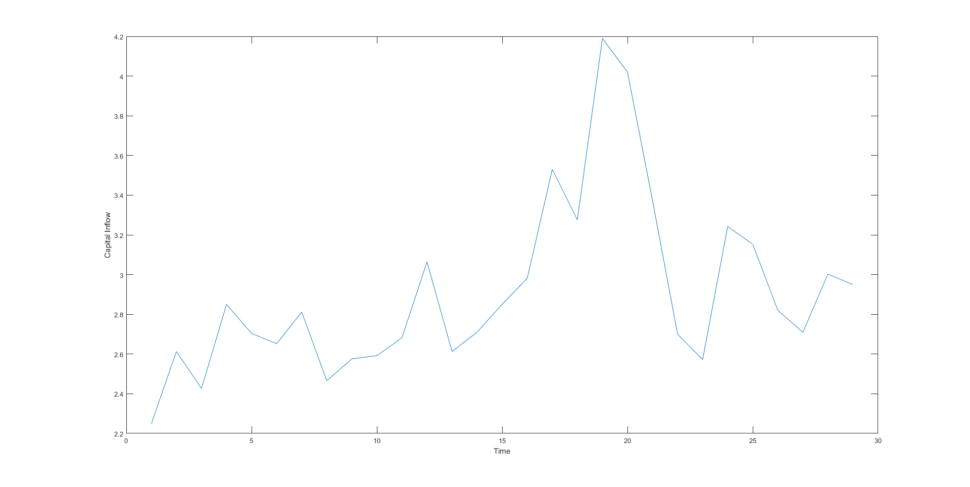
Figure 1: Capital Inflow

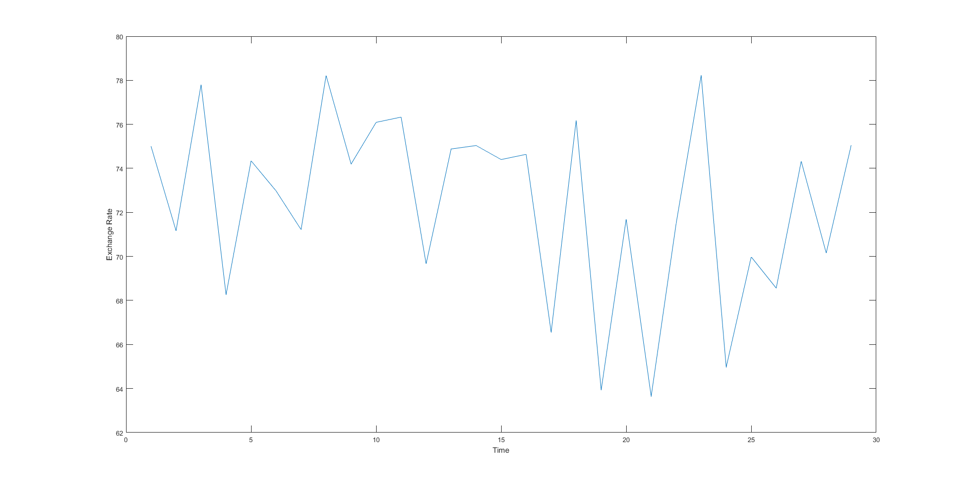
Figure 2: $e_{t}$

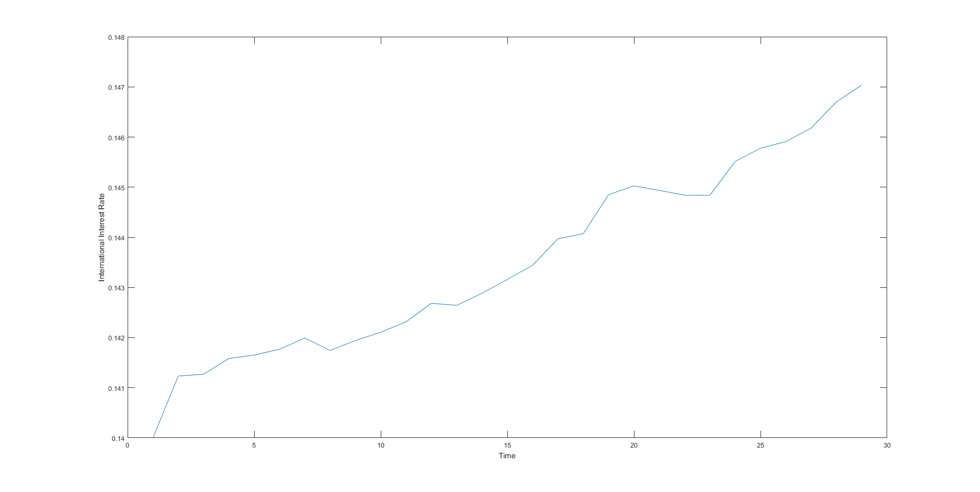
Figure 3: $R_{t}^{*}$

It is evident from the above figures that capital inflow and exchange rate follow stationary pattern with a shift in the trajectory of the former between the period between 15 and 20. The international interest rate shows a rising trend in a small band. This is because of the fact that a static expectation of next period exchange rate with a value less than unity implies banks in the developing country finds it optimal to borrow from the international market. The ever increasing demand for loans raises the interest rate over time. In the process the role of dynamic terms of trade operates via (2.12). If there is an adverse supply shock in the foreign exchange market (due to, say a deficit in the balance of trade) then the second component on the L.H.S. of (2.12) has to fall to match the given value on the R.H.S. This interacts with the R.H.S. of (2.10) to achieve equilibrium in the foreign exchange market. The effect of current period exchange rate becomes more pronounced because the expectation of next period exchange rate is static - invariant to current information set about the future. Eventually in the final equilibrium interest rate effect in each period dominates so that aggregate capital inflow to the developing country hovers around a stationary path. The fluctuation around the stationary path is governed by the stochastic shocks to net exports. In this model balance of trade has a dominant role in the determination of the intertemporal path of foreign capital inflow. As a matter of fact the trajectory of capital inflow is almost a mirror image of the trajectory of the exchange rate.

In Table 3 below we provide the mean and variance of the endogenous variables.

Table 3: Mean and variance of the endogenous variables

Variable	Mean	SD	Coefficient of Variation
$R_{t}^{*}$	0.1444	0.0015	0.0104
$e_{t}$	71.7915	4.4440	0.0619
Capital inflow	3.0516	0.4532	0.1485

The average exchange rate for the period of simulation turns out to be $71.7915$ units of domestic currency per unit of the foreign currency and the interest of the international market is $14.44\%$. The aggregate equilibrium capital inflow to the developing country is 3.0516 units. It may be noted that the mean and standard deviation of the endogenous variables reported in Table 3 are valid for the values of the parameters and initial values of the endogenous variables as in Tables 1 and 2. Any change in one or more of the parameter values generates different dynamic paths of the endogenous variables. Such exercises constitute comparative dynamics of the model. The new mean and standard deviation of the endogenous variables summarize the change in the series corresponding to new parameter values.

3 Comparative Dynamic Analysis

We consider changes in some of the parameter values of interest for a better understanding of the economics of foreign capital inflow with emphasis on the primary focus of the model. It may be noted that for the comparative dynamic analysis we have retained the same realised values of shock to the net export function to make comparisons meaningful. The set of baseline trajectory of the endogenous variables are plotted in black while the new set are plotted in red throughout this paper.

3.1 Change in risk perception of the developed country banks, $\gamma$

An increase in $\gamma$ implies that banks in the developed country perceive a higher risk for a given level of expected profit (see equation (2.2)). In this particular exercise $\gamma$ is raised from 4 to 15. The change corresponds to a dramatic shift in the risk perception and often happens during the episodes of crisis. Then a typical bank in the developed country supplies lower amount of funds in the international market. As a result aggregate supply of foreign loans decreases resulting into increase in the international rate $R_{t}^{*}$. In the final equilibrium capital inflow to the developing country decreases and international rate increases for each $t$.

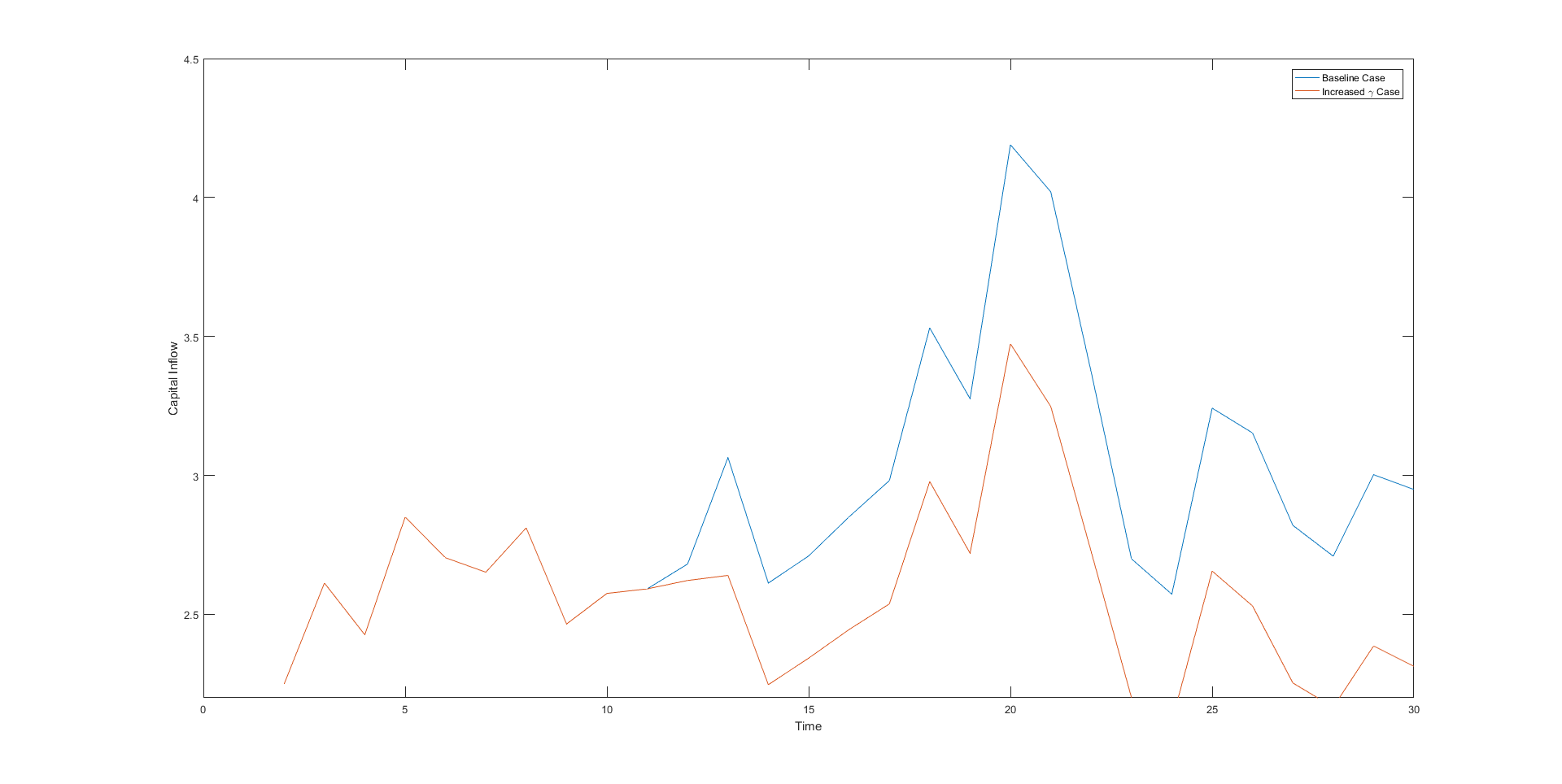
Figure 4: Effect of increased $\gamma$ on capital inflow (Bottom plot for higher $\gamma$)

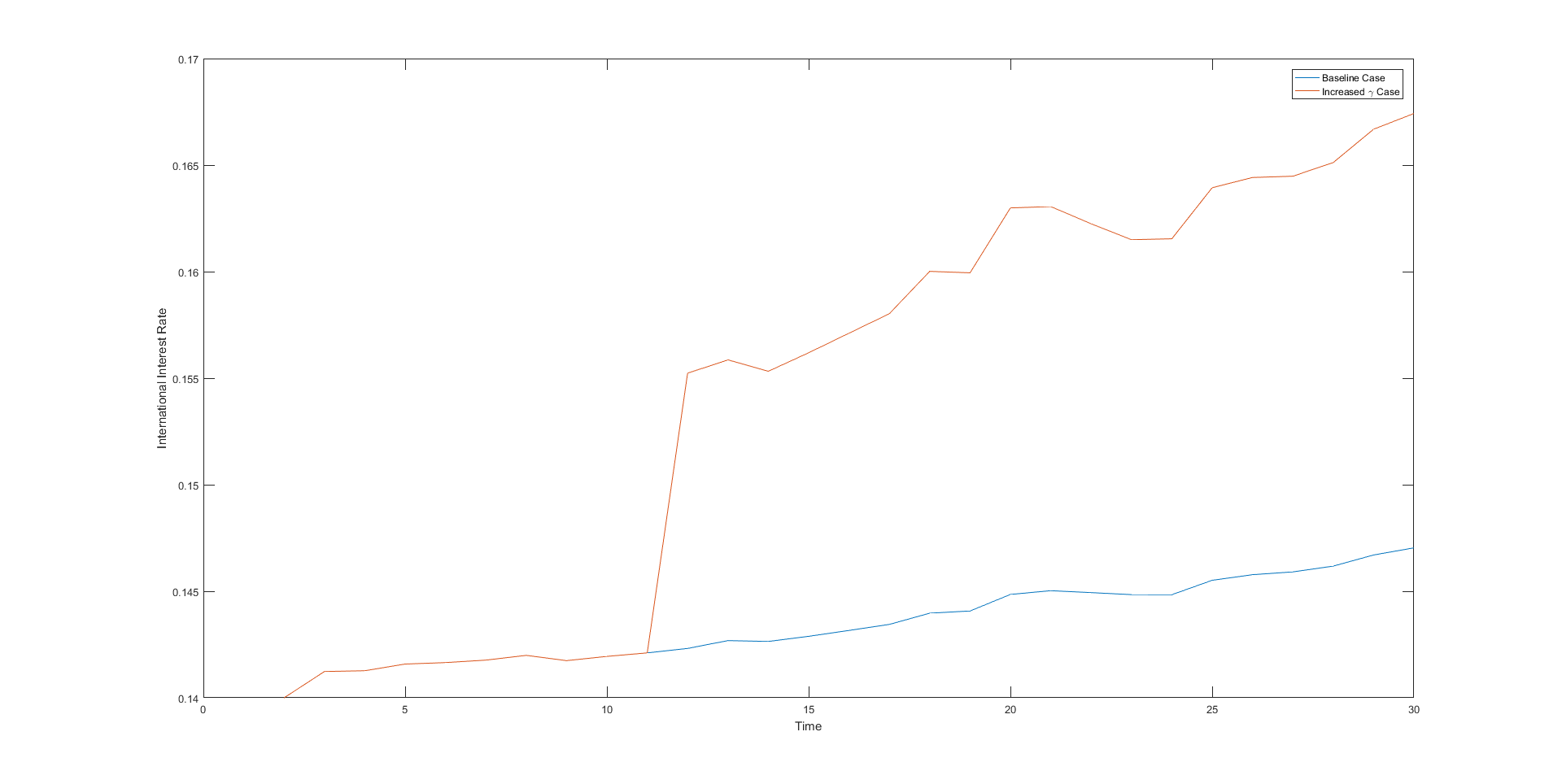
Figure 5: Effect of increased $\gamma$ on $R^{*}_{t}$ (Top plot for higher $\gamma$)

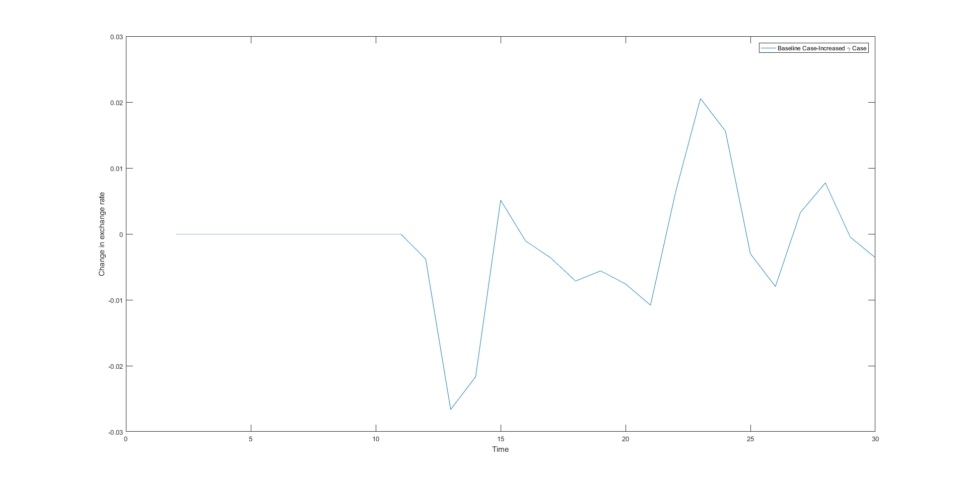
Figure 6: Effect of increased $\gamma$ on $e_{t}$ (difference with baseline)

Figs. 4 and 5 depict the new intertemporal trajectory (in red) of the capital inflow and the international interest rate along with the baseline (in black). The trajectory of capital inflow shows a downward shift from the original trajectory while the international interest rate shifts up. However, there is very little change in the exchange rate. To get a clear picture we plotted the difference of the new exchange rate from its baseline for each $t$ and plotted them in Fig. 6. The trajectory follows a stationary path around zero within a band from -0.027 to 0.02. There is no appreciable change in the exchange rate because the shock does not affect the net exports and so the balance of trade which as we argued earlier has a dominating role in the determination of the equilibrium trajectories.

Table 4: Mean and variance of variables-increased $\gamma$

Variable	Mean	SD	Coefficient of Variation
$R_{t}^{*}$	0.1602	0.0057	0.0356
$e_{t}$	71.7937	4.4425	0.0619
capital inflow	2.5597	0.3543	0.1384

The averages for the new values of the endogenous variables also confirm this. There is a decrease in the average foreign capital inflow from $3.0516$ to $2.5597$ which is expected because of the increase in borrowing rate $R_{t}^{*}$. However, the percentage fall in foreign capital inflow 16.12% is more than the rise in $R_{t}^{*}$ 10.94%. The increase in risk perception, $\gamma$ is 275% from its initial value. The rate of change in the average capital inflow with respect to $\gamma$ is -0.0447 while the rate of change of $R_{t}^{*}$ is 0.00014. The elasticity of capital inflow and interest rate with respect to $\gamma$ are -0.0379 and 0.0014 (evaluated at sample averages). Clearly the sensitivity of capital inflow to risk perception is much higher than the sensitivity of interest rate.

3.2 Effect of a rise in $E_{t}(\frac{e_{t+1}}{e_{t}})$: Expected depreciation of exchange rate

When banks in the developing country (borrowers in the developing country in general) expect a depreciation of exchange rate in the future, meaning an increase in the expected exchange rate vis-à-vis current rate, $E_{t}(\frac{e_{t+1}}{e_{t}})$, cost of borrowing (in terms of foreign currency) increases. This change in expectation leads to a decrease in the demand for foreign borrowing which in turn reduces $R_{t}^{*}$ in the final equilibrium in each period. $E_{t}(\frac{e_{t+1}}{e_{t}})$ is raised from 0.92 to 0.98 (6.52% rise), with no change in the other parameter values. Comparing the new intertemporal trajectory with the baseline trajectory we find that the capital inflow attains a low level trajectory though the nature of the time path remains similar to the baseline trajectory.

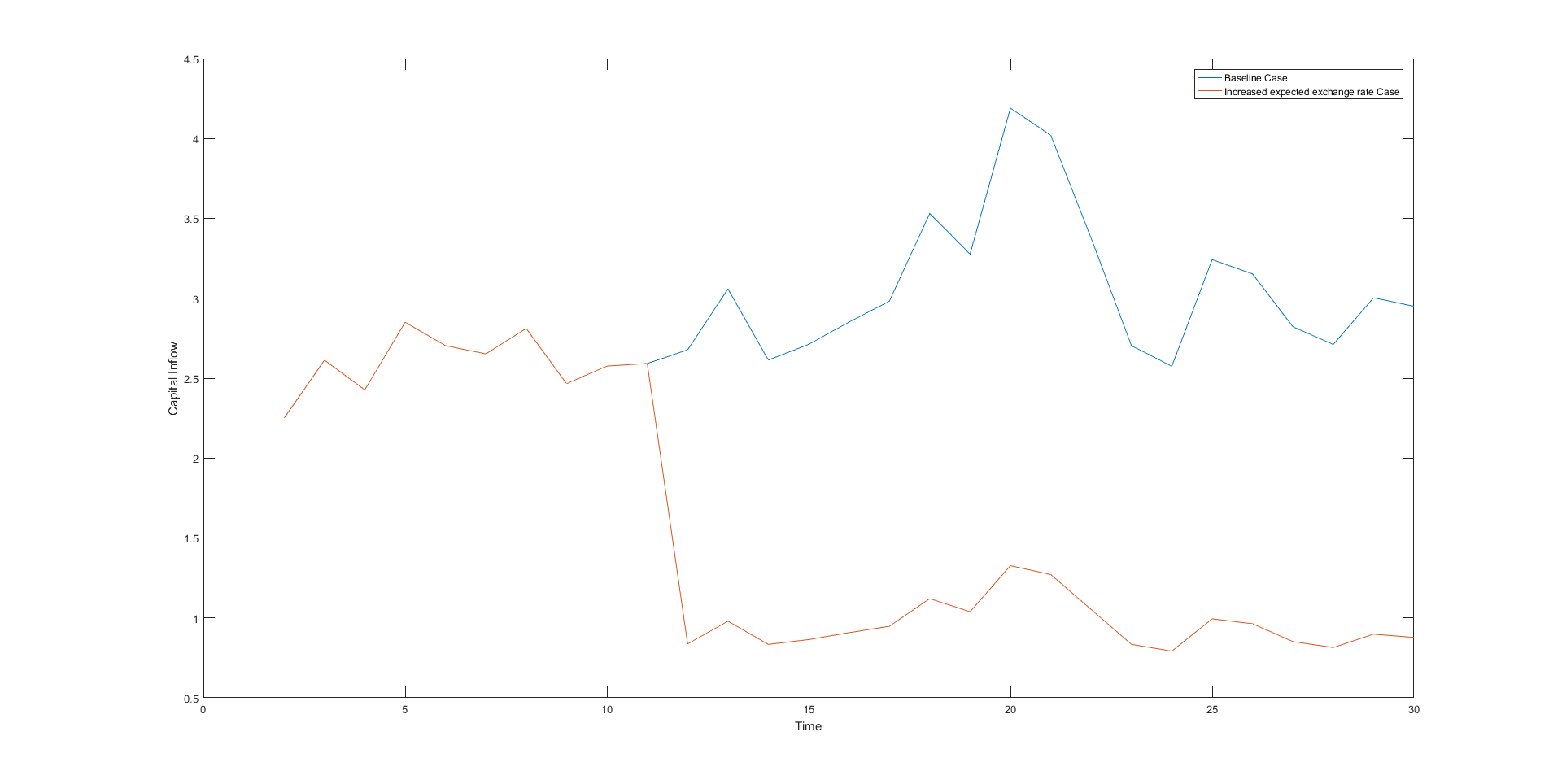
Figure 7: Effect of depreciation of $E(\frac{e_{t+1}}{e_{t}})$ on capital inflow (Bottom plot for higher $E(\frac{e_{t+1}}{e_{t}})$)

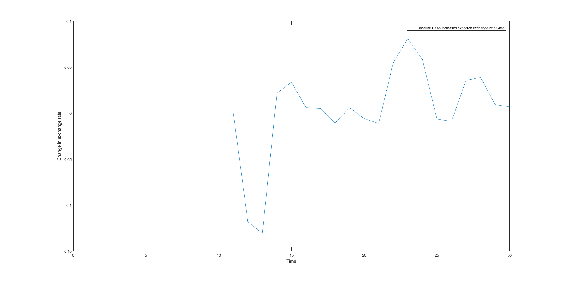
Figure 8: Effect of depreciation of $E(\frac{e_{t+1}}{e_{t}})$ on $e_{t}$ (difference from baseline)

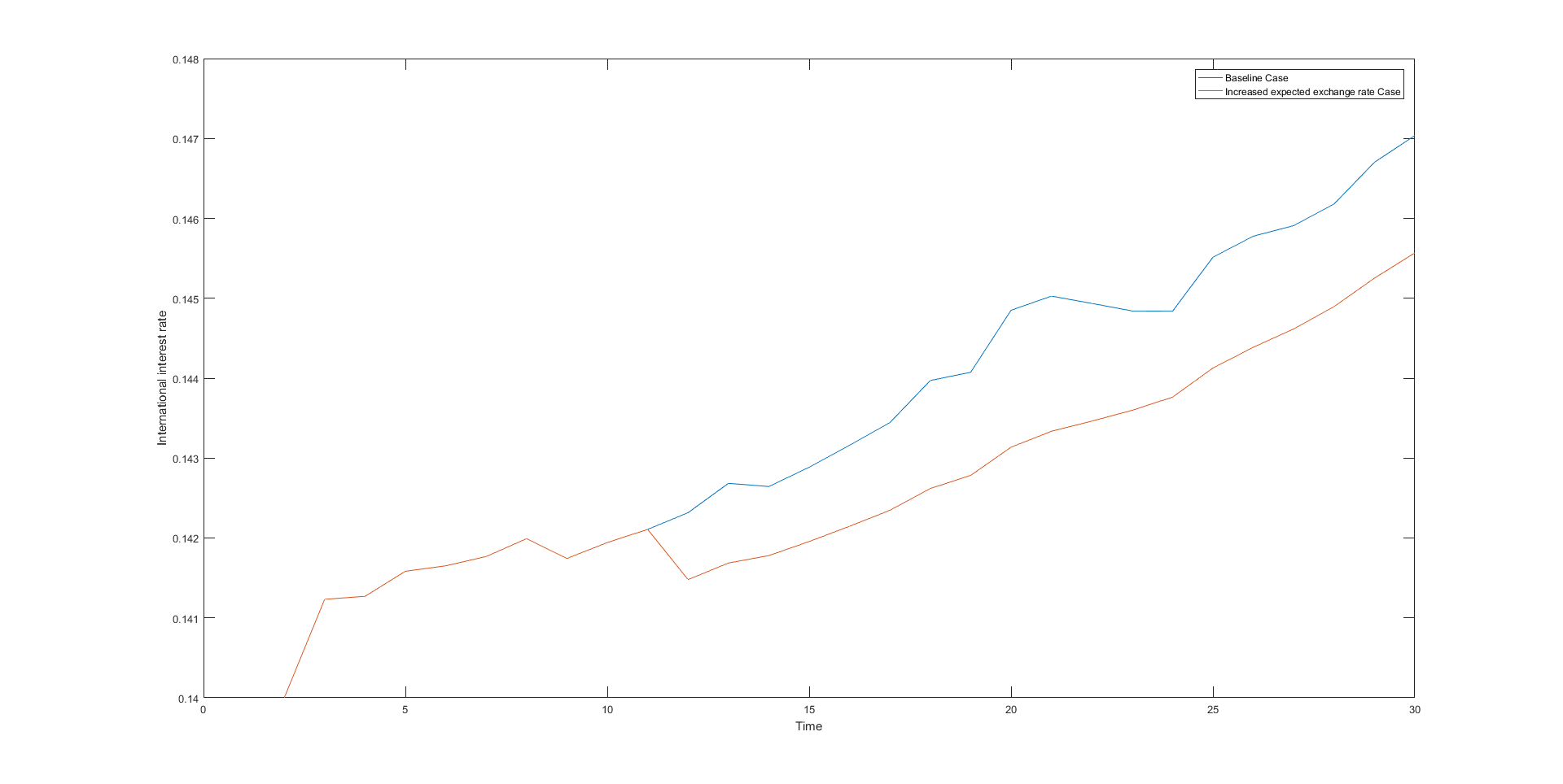
Figure 9: Effect of depreciation of $E(\frac{e_{t+1}}{e_{t}})$ on $R^{*}_{t}$ (Bottom plot for higher $E(\frac{e_{t+1}}{e_{t}})$)

Table 5: Mean and variance of variables - Increased $E(\frac{e_{t+1}}{e_{t}})$

Variable	Mean	SD	Coefficient of Variation
$R_{t}^{*}$	0.1433	0.0013	0.0087
$e_{t}$	71.7883	4.4439	0.0619
capital inflow	1.0399	0.3934	0.3783

Comparing the summary statistics reported in Table 5 with the baseline summary statistics reveals that capital inflow decreases by 65.92% and $R_{t}^{*}$ decreases by 0.76% on an average. The rate of change of capital inflow with respect to expected exchange rate is -33.53 which is much higher than the rate of change of interest rate (-0.0183). The elasticities of capital inflow and interest rate with respect to expected exchange rate are found to be -15.57 and -0.121. The current exchange rate does not change to any appreciable level. Difference of the current exchange rate from the baseline plotted in Fig. 8 shows that the range of variation is not significant (from $-0.14$ to $0.07$). The behaviour of the endogenous variables as depicted in the figures are also confirm from the respective averages over the periods provided in Table 5.

3.3 Decrease in the productivity of the domestic sector of the developing country, $E_{t}(\eta)$

When there is a decrease in the productivity of the domestic sector of the developing country, $E_{t}(\eta_{t})$, profit in the production sector falls which in turn leads to decreased demand for foreign loans by the developing countries. We conduct this exercise by reducing $E_{t}(\eta_{t})$ reduced from 0.85 to 0.70 (roughly 17.64% decrease). Given below the plots of endogenous variables with the new $E_{t}(\eta_{t})$.

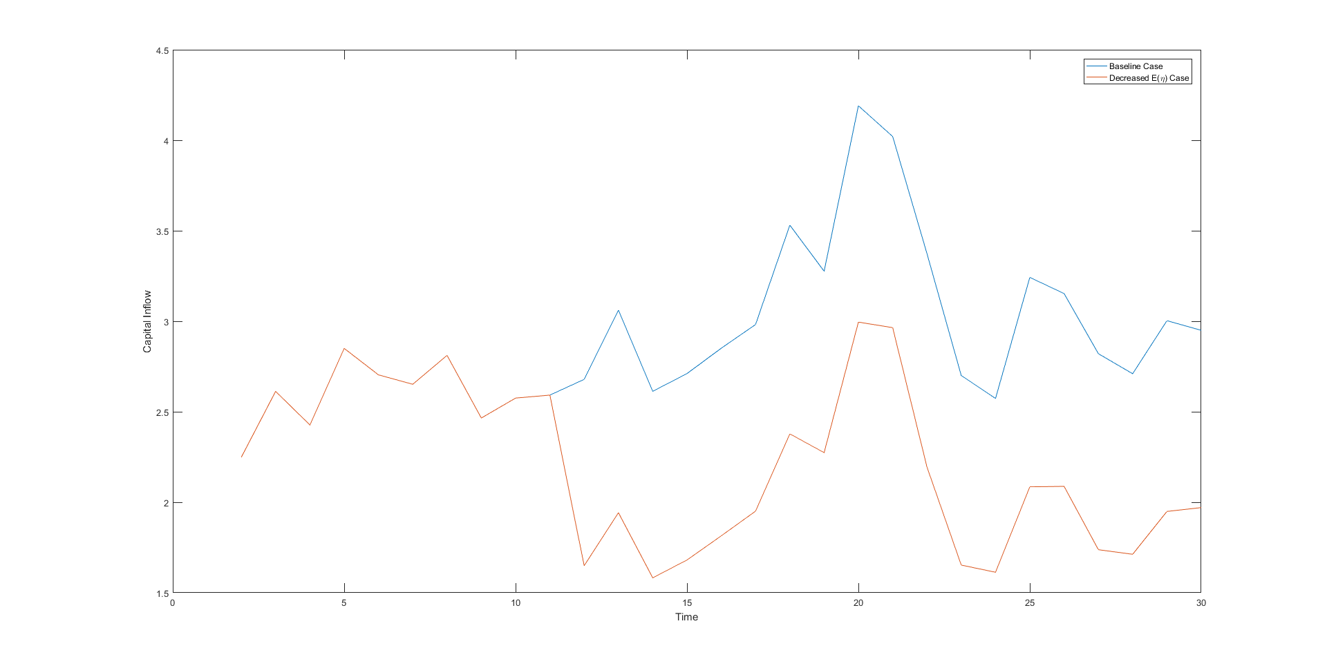
Figure 10: Effect of a lower $E_{t}(\eta)$ on Capital Inflow (Bottom plot for lower $E_{t}(\eta)$)

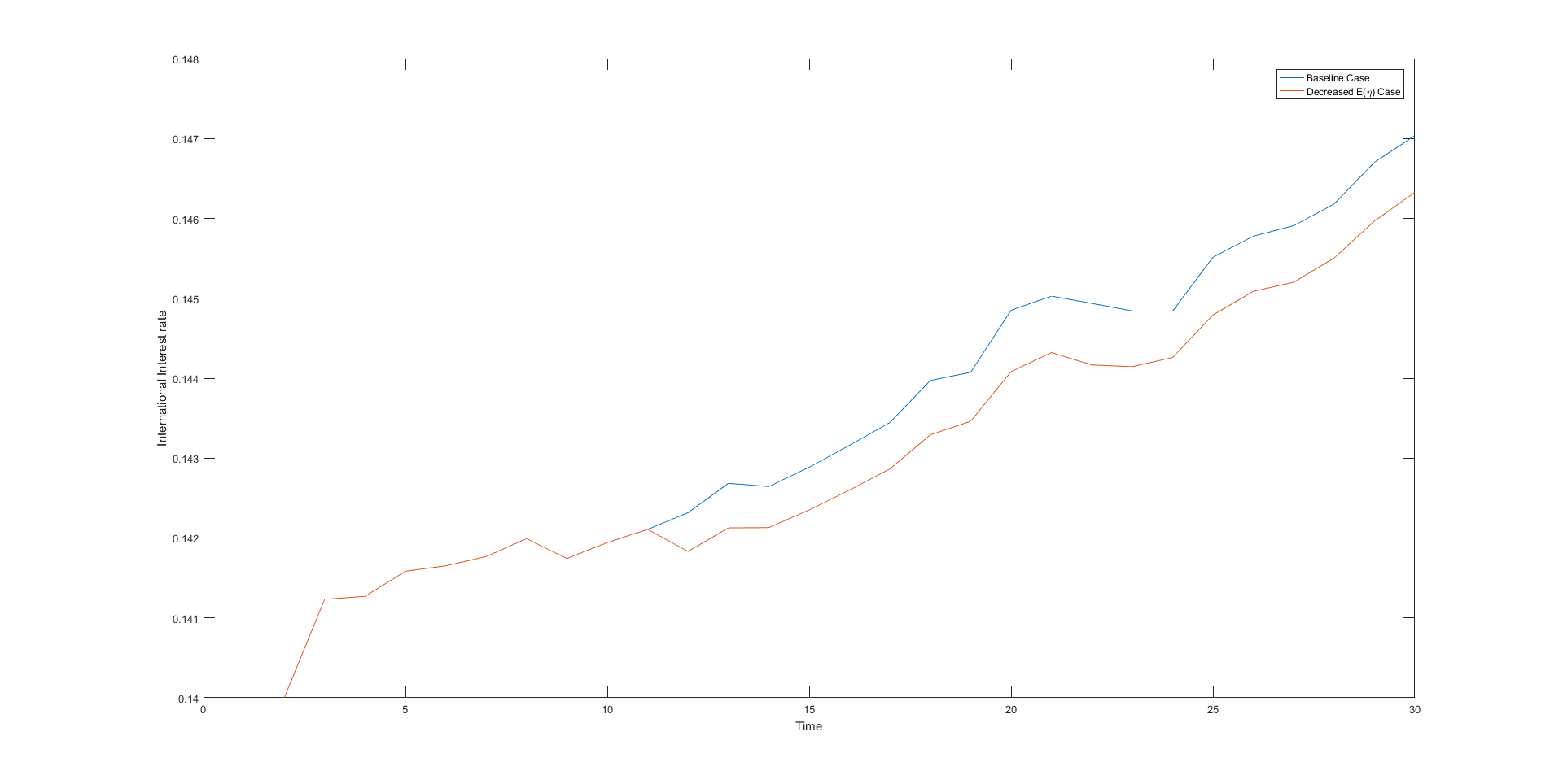
Figure 11: Effect of a lower $E_{t}(\eta)$ on $R_{t}^{*}$ (Bottom plot for lower $E_{t}(\eta)$)

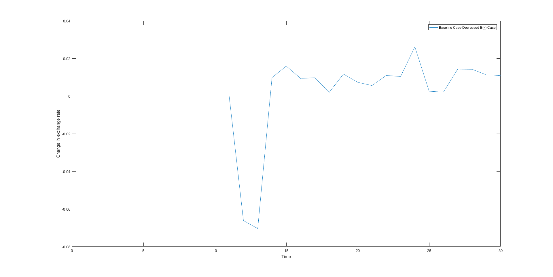
Figure 12: Effect of a lower $E_{t}(\eta)$ on $e_{t}$ (in difference)

From the plot it is seen that the whole trajectory of $R_{t}^{*}$ as well as the trajectory of the capital inflow shift below. Comparing the averages with that of the baseline (see Table 6) it is evident that there is no appreciable change in $e_{t}$ while there is fall in both the capital inflow and $R_{t}^{*}$ by 6.73% and 0.004% respectively. Thus the fall capital inflow is much higher and the fall in $R_{t}^{*}$ is a slightly lower compared to the decrease in productivity, $E(\eta_{t})$. The rate of change of capital inflow with respect to $E(\eta_{t})$ is 6.7 while that for $R_{t}^{*}$ is 0.004 and the corresponding elasticities are 2.05 and 0.022 respectively.

Table 6: Mean and variance of variables-shock to $E_{t}(\eta)$

Variable	Mean	SD	Coefficient of Variation
$R_{t}^{*}$	0.1438	0.0014	0.0096
$e_{t}$	71.7896	4.4437	0.0619
capital inflow	2.0415	0.4212	0.2063

An increase in the production cost in the developing country has similar effect as the decrease in the productivity. Such increases can occur due to increase in the price of inputs, wages, interest rate or price of raw materials. A very common cause of increased production cost arises due to increase in the prices of imported inputs, particularly crude petroleum and generates balance of payments crisis. The comparative dynamic analyses considered above show that the international interest rate is less sensitive to changes in the parameter values than capital inflow. This is true whether the parametric changes occur in the developed country or in the developing country. A comparison of the elasticities of capital inflow and rate of interest in the international loan market with respect to the parameter values reveals that responsiveness with respect to the expected exchange rate in the next period far exceeds the responsiveness with respect to the risk perception of loans of the developed country banks or productivity of the domestic sector of the developing country (borrowing firms in the developing country). However, the behaviour of the current exchange rate is governed by the behaviour of the net exports. It is seldom affected by the change in the expected exchange rate. This is because of the fact that the nature of expectation of the exchange rate is static, expectation of future exchange rate is invariant with respect to behaviour of the current exchange rate.

The above analyses can be useful for an analysis of the potential of financial crisis in this model. All the above three cases have the potential for generating financial crisis when foreign capital inflow drops to a very low level; in the extreme case it can hit the horizontal axis as in Figs. 4 and 10 leading to what can be called sudden stop a la Calvo (1998). As a matter of fact in the case of a sudden stop it is very difficult for the borrowing country to come back to its original position. However, the crisis, in this model does not occur because of imperfection in the loan market resulting into binding finance constraints for firms which becomes profound with goods price rigidity as in Aghion et al(2000). It is not the fallout of classic problem of moral hazard or adverse selection (Krugman, 1998). Nor it is (mis)information issue that has been ascribed very important role in the sense of herd behaviour discussed by Kindleberger (1978) and formally modelled by Banerjee (1992).

We have shown that a favourable foreign capital inflow can turn into a crisis even when macroeconomic fundamentals are good. In view of the such vulnerability of unrestricted capital flow to financial crisis eminent economists such as Bhagwati (1998), Ostroy et al (2010), Rodrick (1998) have suggested policy to tax capital out flow, such as Tobin type tax in general even when macroeconomic fundamentals show good performance and Sen (2006) in particular has argued against full capital account convertibility for the Indian economy.

4 Conclusion

The study addresses the economics of foreign capital inflow based on trade theoretic explanation operating via terms of trade effect in a dynamic context. The model is set up and solved in a two country group framework - developing or borrowing group and developed or lending group. Each individual agent in both the country groups chooses her respective loan portfolio for each period by optimization of an intertemporal objective function of mean-variance variety. The equilibrium in the loan market together with the foreign exchange market solves the endogenous variables of the model using numerical methods. Net exports which constitutes the supply side of the foreign exchange market dominates intertemporal trajectory of endogenous variables. Simulation exercises are then conducted to derive comparative dynamic results to assess the impact of shocks to parameters of the model on the intertemporal trajectory of the endogenous variables, viz. international interest rate, foreign capital inflow and exchange rate.

Given the structure of the model a change in the risk perception in the developed country reduces capital inflow to the developing country group as a whole. An increase in the expected exchange rate vis-à-vis the current exchange rate raises the effective cost of foreign loans leading to a decrease in demand which in the final equilibrium also reduces the international interest rate. A fall in the productivity in the domestic sector of the developing country leads to a fall in foreign capital inflow and a fall in the international interest rate. However, the responsiveness with respect to expected exchange rate vis-à-vis current exchange rate is much more compared to the other comparative dynamic analyses considered here.

The paper can be extended in several directions. A restrictive assumption of the model is static expectation of exchange rate. An extension with endogenous determination of expected exchange rate is capable to add richer dynamics to the model. Another interesting extension could be the endogeneity of risk of default that is dependent on the outstanding borrowing of the developing countries. Finally, a multi country extension within the borrowing country group can be undertaken to show the contagion effect when a shock originating in one of the borrowing countries spreads to the other members of the group.

5 Appendix A

Proof of Theorem 1:  From (2.3)

$$a+bF_{t}+cF_{t}^{2}=max_{\mu_{t}}\{\Omega_{t}^{D}+B^{D}E_{t}(V^{D}(F_{t+1})\},$$

where

$$\Omega_{t}^{D}=F_{t}(1-\mu_{t})(1+R_{t}^{D})+F_{t}\mu_{t}(1+R_{t}^{*})E_{t}(\epsilon_{t})-(\gamma/2)F_{t}^{2}\mu_{t}^{2}(1+R_{t}^{*)^{2}}V_{t}(\epsilon_{t})$$

and

$$E_{t}(F_{t+1})=F_{t}[(1-\mu_{t})(1+R_{t}^{D})+\mu_{t}(1+R_{t}^{*})E_{t}(\epsilon_{t})]-(1+r_{t}^{D})K_{t}^{D}+K_{t+1}^{D}.$$

To solve this, denote $M_{t}^{D}=\Omega_{t}^{D}+B^{D}[a+bE_{t}(F_{t+1})+cE_{t}(F_{t+1}^{2})]$, then the value function takes the form,

$$V^{D}(F_{t})=\mbox{ma$x_{\mu_{t}}$\{$M_{t}^{D}\}$}.$$

First order condition to the above equation yields

$$\frac{\partial M_{t}^{D}}{\partial\mu_{t}^{*}}|\mu_{t}^{*}=0.$$ (5.1)

Now,

$$\frac{\partial\Omega_{t}^{D}}{\partial\mu_{t}^{*}}=-F_{t}(1+R_{t}^{D})+F_{t}(1+R_{t}^{*})E_{t}(\epsilon_{t})-\gamma F_{t}^{2}\mu_{t}(1+R_{t}^{*})^{2}V_{t}(\epsilon_{t}).$$

$$\Rightarrow\ \ \ \frac{\partial E_{t}(F_{t+1})}{\partial\mu_{t}^{*}}=-F_{t}(1+R_{t}^{D})+F_{t}(1+R_{t}^{*})E_{t}(\epsilon_{t}).$$

$$\Rightarrow\ \ \ E_{t}(F_{t+1}^{2})=V_{t}(F_{t+1})+(E_{t}(F_{t+1}))^{2}.$$

Now,

$$\frac{\partial(E_{t}(F_{t+1}))^{2}}{\partial\mu_{t}^{*}}=2E_{t}(F_{t+1})\frac{\partial E_{t}(F_{t+1})}{\partial\mu_{t}^{*}}$$

and,

$$V_{t}(F_{t+1})=\mu_{t}^{2}(1+R_{t}^{*})^{2}F_{t}^{2}V_{t}(\epsilon_{t}).$$

Thus,

$$\frac{\partial V_{t}(F_{t+1})}{\partial\mu_{t}^{*}}=2\mu_{t}(1+R_{t}^{*})^{2}F_{t}^{2}V_{t}(\epsilon_{t})$$

$$\Rightarrow\ \ \ \frac{\partial M_{t}^{D}}{\partial\mu_{t}^{*}}|\mu_{t}^{*}=\frac{\partial\Omega_{t}^{D}}{\partial\mu_{t}^{*}}+B^{D}b\frac{\partial E_{t}(F_{t+1})}{\partial\mu_{t}^{*}}+B^{D}c\frac{\partial V_{t}(F_{t+1})}{\partial\mu_{t}^{*}}+B^{D}c\frac{\partial(E_{t}(F_{t+1}))^{2}}{\partial\mu_{t}^{*}}.$$

This implies,

$$0 = -F_{t}(1+R_{t}^{D})+F_{t}(1+R_{t}^{*})E_{t}(\epsilon_{t})-\gamma F_{t}^{2}\mu_{t}(1+R_{t}^{*})^{2}V_{t}(\epsilon_{t})$$

$$+B^{D}b[-F_{t}(1+R_{t}^{D})+F_{t}(1+R_{t}^{*})E_{t}(\epsilon_{t})]+B^{D}c[2\mu_{t}(1+R_{t}^{*})^{2}F_{t}^{2}V_{t}(\epsilon_{t})]$$

$$+2B^{D}c[F_{t}[(1-\mu_{t})(1+R_{t}^{D})+\mu_{t}(1+R_{t}^{*})E_{t}(\epsilon_{t})]-r_{tk}^{D}]$$

$$\times[-F_{t}(1+R_{t}^{D})+F_{t}(1+R_{t}^{*})E_{t}(\epsilon_{t})].$$

Rearranging,

$$\mu_{t}^{*} = \frac{F_{t}Z_{t}[(1+B^{D}b)+2B^{D}cF_{t}(1+R_{t}^{D})-2B^{D}cr_{tk}^{D}]}{F_{t}^{2}[\gamma(1+R_{t}^{*})^{2}V_{t}(\epsilon_{t})-2B^{D}c(Z_{t}^{2}+(1+R_{t}^{*})^{2}V_{t}(\epsilon_{t}))]}$$ (5.3)

$$= \frac{Z_{t}[(1+B^{D}b)+2B^{D}cF_{t}(1+R_{t}^{D})-2B^{D}cr_{tk}^{D}]}{F_{t}[\gamma(1+R_{t}^{*})^{2}V_{t}(\epsilon_{t})-2B^{D}c(Z_{t}^{2}+(1+R_{t}^{*})^{2}V_{t}(\epsilon_{t}))]}$$

with

$$Z_{t}=[(1+R_{t}^{*})E_{t}(\epsilon_{t})-(1+R_{t}^{D})]$$ (5.4)

and

$$r_{tk}^{D}=(1+r_{t})K_{t}^{D}-K_{t+1}^{D},$$ (5.5)

where $b$ and $c$ are determined as given below. Let $\mu_{t}^{*}$be the optimum portfolio, then the optimum portfolio satisfies $a+bF_{t}+cF_{t}^{2}=\Omega_{t}^{D}(F_{t},\mu_{t}^{*})+B^{D}E_{t}(V(F_{t+1})(\mu_{t}^{*}))$ from equation (2.3) This equation holds for every $F_{t}$, so $a$, $b$, $c$ are determined by comparing coefficients of $F_{t}$ , $F_{t}^{2}$ and constant on both the sides of the equation. This implies

$$a+bF_{t}+cF_{t}^{2} = F_{t}[(1-\mu_{t}^{*})(1+R_{t}^{D})+\mu_{t}^{*}(1+R_{t}^{*})E_{t}(\epsilon_{t})]-\frac{\gamma}{2}F_{t}^{2}{\mu_{t}^{*}}^{2}(1+R_{t}^{*})^{2}V_{t}(\epsilon)+B^{D}a$$ (5.6)

$$+B^{D}b[F_{t}[(1-\mu_{t}^{*})(1+R_{t}^{D})+\mu_{t}^{*}(1+R_{t}^{*})E_{t}(\epsilon_{t})]-(1+r_{t}^{D})K_{t}^{D}+K_{t+1}^{D}]$$

$$+B^{D}c[(E_{t}(F_{t+1}))^{2}+V_{t}(F_{t+1})].$$

This is so because $E_{t}(F_{t+1}^{2})=(E_{t}(F_{t+1}))^{2}+V_{t}(F_{t+1})$ Comparing the coefficients of $F_{t}^{2}$ on both the sides of the equation, the following equality is obtained:

$$c=(1+R_{t}^{*})^{2}V_{t}(\epsilon_{t})\left(\frac{2B^{D}c(1+R^{D}_{t})Z_{t}}{\mu_{denom}}\right)^{2}(-(\gamma/2)+B^{D}c)+(1+R^{D})^{2}B^{D}c+\frac{(2B^{D}c(1+R^{D}_{t})Z_{t})^{2}}{\mu_{denom}},$$

where $\mu_{denom}=(\gamma-2B^{D}c)(1+R_{t}^{*})^{2}V_{t}(\epsilon_{t})-2B^{D}cZ_{t}^{2}$. This yields,

$$\mu_{denom}^{2}c(1-B^{D}(1+R_{t}^{D})^{2}) = (2B^{D}c(1+R^{D}_{t})Z_{t})^{2}[\mu_{denom}-(1/2)(\gamma-2B^{D}c)(1+R_{t}^{*})^{2}V_{t}(\epsilon_{t})]$$

$$\Rightarrow$$

$$(A-cE)^{2}(1-T) = 2cZ_{t}^{2}B^{D}T(A-cE_{1})$$

$$\Rightarrow (\mbox{ as }c\neq 0,\mbox{ otherwise the value function would be linear }$$

$$(A^{2}+c^{2}E^{2}-2cAE)(1-T) = 2cZ_{t}^{2}B^{D}T(A-cE_{1})$$

$$\Rightarrow$$

$$0 = c^{2}(E^{2}(1-T)+2Z_{t}^{2}B^{D}TE_{1})-2c(AE(1-T)+Z_{t}^{2}B^{D}TA)+A^{2}(1-T)$$

where $A=\gamma(1+R_{t}^{*})^{2}V_{t}(\epsilon_{t})$,  $E=2B^{D}(Z_{t}^{2}+(1+R_{t}^{*})^{2}V_{t}(\epsilon_{t}))=2B^{D}(Z_{t}^{2}+\frac{A}{\gamma})$,  $T=B^{D}(1+R_{t}^{D})^{2}$  and  $E_{1}=2B^{D}(Z_{t}^{2}+\frac{A}{2\gamma})$. Hence, Note, since $A$, $E$ and $T$ all are positive, the coefficient of $c$ in (5) is negative. Therefore, if $0<T\leq 1$, then all solution of $c$ are positive real, as the discriminant is positive, since for $0<T\leq 1$,  $A^{2}E^{2}(1-T)^{2}=A^{2}E^{2}(1-T)^{2}$,  $2B^{D}Z_{t}^{2}A^{2}ET(1-T)\geq 2B^{D}Z_{t}^{2}A^{2}E_{1}T(1-T)$  and  $(B^{D})^{2}Z_{t}^{4}A^{2}T^{2}>0$. Hence, the necessary condition is $T>1$. But then the discriminant may not always be positive as the 2nd condition may not always hold and the coefficient of $c^{2}$ may also be negative. So, the main idea would be to choose $B^{D}$, such that $T>1$, i.e, coefficient of $c^{0}$ is negative, but the coefficient of $c^{2}$ is positive. For $T>1$, when coefficient of $c^{2}$ is positive then there exists exactly one solution of $c$ which is negative. Therefore $c<0$ if and only if $B^{D}(1+R_{t}^{D})^{2}>1$  and

$$(1+R_{t}^{D})^{2}(Z_{t}^{2}+(1+R_{t}^{*})^{2}V_{t}(\epsilon_{t}))^{2} > T[(Z_{t}^{2}+(1+R_{t}^{*})^{2}V_{t}(\epsilon_{t}))^{2}-Z_{t}^{2}(Z_{t}^{2}+(1/2)(1+R_{t}^{*})^{2}V_{t}(\epsilon_{t}))^{2}]$$

$$= T[(3/2)Z_{t}^{2}(1+R_{t}^{*})^{2}V_{t}(\epsilon_{t})+((1+R_{t}^{*})^{2}V_{t}(\epsilon_{t}))^{2}$$

$$\Leftrightarrow B^{D}(1+R_{t}^{D})^{2}<\frac{(Z_{t}^{2}+(1+R_{t}^{*})^{2}V_{t}(\epsilon_{t}))^{2}}{(3/2)Z_{t}^{2}(1+R_{t}^{*})^{2}V_{t}(\epsilon_{t})+((1+R_{t}^{*})^{2}V_{t}(\epsilon_{t}))^{2}}.$$

For the coefficient of $F_{t}$,

$$b = 2B^{D}c\frac{Z_{t}^{2}(1+R_{t}^{D})}{\mu_{denom}}+(1+R_{t}^{D})-\frac{\gamma}{2}(1+R_{t}^{*})^{2}V_{t}(\epsilon_{t})4B^{D}c(1+R_{t}^{D})\frac{Z_{t}^{2}}{\mu_{denom}^{2}}[(1+B^{D}b)-2B^{D}cr_{tk}^{D}]$$ (5.10)

$$+B^{D}b[(1+R^{D})+\frac{Z_{t}^{2}}{\mu_{denom}^{2}}2B^{D}c(1+R_{t}^{D})]+B^{D}c[\frac{2Z_{t}^{2}(1+R_{t}^{D})}{\mu_{denom}}[(1+B^{D}b)-2B^{D}cr_{tk}^{D}]$$

$$+\frac{2Z_{t}^{4}(1+R_{t}^{D})}{\mu_{denom}^{2}}2B^{D}c[(1+B^{D}b)-2B^{D}cr_{tk}^{D}]-2r_{tk}^{D}[(1+R_{t}^{D})+2B^{D}c\frac{Z_{t}^{2}(1+R_{t}^{D})}{\mu_{denom}}]]$$

$$+B^{D}c(1+R_{t}^{*})^{2}V_{t}(\epsilon_{t})4B^{D}c(1+R_{t}^{D})\frac{Z_{t}^{2}}{\mu_{denom}^{2}}[(1+B^{D}b)-2B^{D}cr_{tk}^{D}]$$

$$= (1+R_{t}^{D})(1+2B^{D}c\frac{Z_{t}^{2}}{\mu_{denom}})[(1+B^{D}b)-2B^{D}cr_{tk}^{D}]$$

$$+2B^{D}c(1+R_{t}^{D})\frac{Z_{t}^{2}}{\mu_{denom}}(1+2B^{D}c\frac{Z_{t}^{2}}{\mu_{denom}})[(1+B^{D}b)-2B^{D}cr_{tk}^{D}]$$

$$+(1+R_{t}^{*})^{2}V_{t}(\epsilon_{t})4B^{D}c\frac{Z_{t}^{2}}{\mu_{denom}^{2}})[(1+B^{D}b)-2B^{D}cr_{tk}^{D}][B^{D}c-\frac{\gamma}{2}]$$

$$= [(1+B^{D}b)-2B^{D}cr_{tk}^{D}](1+R_{t}^{D})(1+2B^{D}c\frac{Z_{t}^{2}}{\mu_{denom}})(1+2B^{D}c\frac{Z_{t}^{2}}{\mu_{denom}})$$

$$+[(1+B^{D}b)-2B^{D}cr_{tk}^{D}](1+R_{t}^{*})^{2}V_{t}(\epsilon_{t})4B^{D}c(1+R_{t}^{D})\frac{Z_{t}^{2}}{\mu_{denom}^{2}})[B^{D}c-\frac{\gamma}{2}]$$

$$= [(1+B^{D}b)-2B^{D}cr_{tk}^{D}][(1+R_{t}^{D})(1+2B^{D}c\frac{Z_{t}^{2}}{\mu_{denom}})^{2}$$

$$-(\frac{\gamma}{2}-B^{D}c)(1+R_{t}^{*})^{2}V_{t}(\epsilon_{t})4B^{D}c(1+R_{t}^{D})\frac{Z_{t}^{2}}{\mu_{denom}^{2}}].$$

This implies,

$$b(1-B^{D}L) = (1-2B^{D}cr_{tk}^{D})L$$

$$\Rightarrow$$

$$b = \frac{(1-2B^{D}cr_{tk}^{D})L}{1-B^{D}L},$$ (5.11)

where

$$L = (1+R_{t}^{D})\left(1+\frac{2B^{D}cZ_{t}^{2}}{\mu_{denom}}\right)^{2}-(\gamma-2B^{D}c)(1+R_{t}^{*})^{2}V_{t}(\epsilon_{t})(1+R_{t}^{D})\frac{2B^{D}cZ_{t}^{2}}{\mu_{denom}^{2}}$$ (5.12)

$$= (1+R_{t}^{D})\left(1-\frac{-2B^{D}cZ_{t}^{2}}{\mu_{denom}}\right)^{2}+(1+R_{t}^{D})\frac{(\gamma-2B^{D}c)(1+R_{t}^{*})^{2}V_{t}(\epsilon_{t})}{\mu_{denom}}\frac{-2B^{D}cZ_{t}^{2}}{\mu_{denom}}$$

$$= (1+R_{t}^{D})\left(1-\frac{-2B^{D}cZ_{t}^{2}}{\mu_{denom}}\right)^{2}+(1+R_{t}^{D})\left(1-\frac{-2B^{D}cZ_{t}^{2}}{\mu_{denom}}\right)\frac{-2B^{D}cZ_{t}^{2}}{\mu_{denom}},$$

since $\mu_{denom}-(\gamma-2B^{D}c)(1+R_{t}^{*})^{2}V_{t}(\epsilon_{t})=-2B^{D}cZ_{t}^{2}$. Hence,

$$L = (1+R_{t}^{D})\left(1-\frac{-2B^{D}cZ_{t}^{2}}{\mu_{denom}}\right)\left[1-\frac{-2B^{D}cZ_{t}^{2}}{\mu_{denom}}+\frac{-2B^{D}cZ_{t}^{2}}{\mu_{denom}}\right]$$ (5.13)

$$= (1+R_{t}^{D})\left(1-\frac{-2B^{D}cZ_{t}^{2}}{\mu_{denom}}\right).$$

This immediately implies that $B^{D}L<1$, as $z$ is negative and $\frac{-2B^{D}cZ_{t}^{2}}{\mu_{denom}}<1$. Also, note

$$1+B^{D}b=\frac{(1-2B^{D}cr_{tk}^{D}(B^{D}L))}{1-B^{D}L}.$$

Positivity of the $\mu_{t}^{*}$ may be found from the condition as given below.

$$\mu_{t}^{*}>0 \Leftrightarrow \frac{1-2B^{D}cr_{tk}^{D}(B^{D}L)}{1-B^{D}L}+2B^{D}c[F_{t}(1+R_{t}^{D})-r_{tk}^{D}]>0$$ (5.14)

$$\Leftrightarrow 1-2B^{D}cr_{tk}^{D}(B^{D}L)+2B^{D}c(1-B^{D}L)[F_{t}(1+R_{t}^{D})-r_{tk}^{D}]>0$$

$$\Leftrightarrow 1-2B^{D}cr_{tk}^{D}+2B^{D}c(1-B^{D}L)[F_{t}(1+R_{t}^{D})]>0$$

$$\Leftrightarrow 2B^{D}c[r_{tk}^{D}-(1-B^{D}L)[F_{t}(1+R_{t}^{D})]]<1.$$

If $r_{tk}^{D}>(1-B^{D}L)[F_{t}(1+R_{t}^{D})]$, then it always holds as $c<0$. This should be the case, as it means $F_{t}$, is tool small compared to $r_{tk}^{D}$. On the other hand, if $r_{tk}^{D}<(1-B^{D}L)[F_{t}(1+R_{t}^{D})]$, which is often the case, then there exists $\gamma_{1}>0$ such that, $\gamma<\gamma_{1}$ would imply the last condition, as $c$ is linear in $\gamma$. This means if the loan do not have too high a risk premium then $\mu_{t}^{*}>0$.

Again, the condition for $\mu_{t}^{*}<1$ may be found from below:

$$\mu_{t}^{*}<1 \Leftrightarrow Z_{t}\left(\frac{1-2B^{D}cr_{tk}^{D}(B^{D}L)}{1-B^{D}L}+2B^{D}c[F_{t}(1+R_{t}^{D})-r_{tk}^{D}]\right)<\mu_{denom}F_{t}$$ (5.15)

$$\Leftrightarrow Z_{t}\left((1-2B^{D}cr_{tk}^{D}(B^{D}L))+2B^{D}c(1-B^{D}L)[F_{t}(1+R_{t}^{D})-r_{tk}^{D}]\right)<\mu_{denom}F_{t}(1-B^{D}L)$$

$$\Leftrightarrow Z_{t}\left((1-2B^{D}cr_{tk}^{D})+2B^{D}c(1-B^{D}L)[F_{t}(1+R_{t}^{D})]\right)<\mu_{denom}F_{t}(1-B^{D}L)$$

$$\Leftrightarrow Z_{t}<F_{t}(1-B^{D}L)\mu_{denom}+2B^{D}cZ_{t}[r_{tk}^{D}-(1-B^{D}L)F_{t}(1+R_{t}^{D})].$$

Since $\mu_{denom}$ is linear in $\gamma$, as $c$ is, from (5.14) it is clear that there exists $0<\gamma_{0}<\gamma_{1}$, such that for $\gamma>\gamma_{0}$ the last condtion holds. This means if the riskpremium is to low then there is always a possibility of over-subscription of lending.

Hence the proof of existence of $\mu^{*}\in(0,1)$  for  $\gamma\in(\gamma_{0},\gamma_{1})$. Upper bound $\gamma_{1}$ may be infinity if $F_{t}$ remains too small.

6 Appendix B

Proof of Theorem 2:  To solve the maximization problem, denote

$$M_{t}^{U}=\Omega_{t}^{U}+B^{U}E_{t}(V^{U}(G_{t+1})).$$

Then

$$V^{U}(G_{t})=max_{\lambda_{t}}M_{t}^{U}.$$

First order condition for maximization implies,

$$\frac{\partial M_{t}^{U}}{\partial\lambda_{t}}{\mid}_{\lambda_{t}=\lambda_{t}^{*}}=0$$ (6.1)

Now,

$$\frac{\partial\Omega_{t}^{U}}{\partial\lambda_{t}}=K_{t}^{U}A_{t}+\beta\lambda_{t}K_{t}^{U^{2}}(1+R_{t}^{*})^{2}V_{t}(\frac{e_{t+1}}{e_{t}})$$

where,

$$A_{t}=(1+r_{t}^{U})-(1+R_{t}^{*})E_{t}(\frac{e_{t+1}}{e_{t}}).$$

Further,

$$E_{t}(G_{t+1})=E_{t}(\eta_{t})(1+R_{t}^{U})G_{t}-K_{t}^{U}[(1-\lambda_{t})(1+r_{t}^{U})+\lambda_{t}(1+R_{t}^{*})E_{t}(\frac{e_{t+1}}{e_{t}})]+K_{t+1}^{U}.$$

So,

$$\frac{\partial E_{t}(G_{t+1})}{\partial\lambda_{t}}=K_{t}^{U}A_{t},$$

and, $E_{t}(G_{t+1}^{2})=(E_{t}(G_{t+1}))^{2}+V_{t}(G_{t+1})$.

Now,

$$\frac{\partial(E_{t}(G_{t+1})^{2}}{\partial\lambda_{t}}=2E_{t}(G_{t+1})\frac{\partial E_{t}(G_{t+1}}{\partial\lambda_{t}}$$

$$\Rightarrow\ \ \ V_{t}(G_{t+1})=K_{t}^{U^{2}}\lambda_{t}^{2}(1+R_{t}^{*})^{2}V_{t}(\frac{e_{t+1}}{e_{t}})+V_{t}(e^{\int_{0}^{t}\theta_{u}^{2}du}ta_{t})G_{t}^{2}(1+R_{t}^{U})^{2}.$$

Thus

$$\frac{\partial V_{t}(G_{t+1})}{\partial\lambda_{t}}=2K_{t}^{U^{2}}\lambda_{t}(1+R_{t}^{*})^{2}V_{t}(\frac{e_{t+1}}{e_{t}}).$$

$$\Rightarrow\ \ \ \frac{\partial M_{t}^{U}}{\partial\lambda_{t}}=\frac{\partial\Omega_{t}^{U}}{\partial\lambda_{t}}+B^{U}y\frac{\partial E_{t}(G_{t+1})}{\partial\lambda_{t}}+B^{U}z\frac{\partial V_{t}(G_{t+1})}{\partial\lambda_{t}}+B^{U}z\frac{\partial(E_{t}(G_{t+1}))^{2}}{\partial\lambda_{t}}.$$

This implies,

$$0 = K_{t}^{U}A_{t}-\beta\lambda_{t}K_{t}^{U^{2}}(1+R_{t}^{*})^{2}V_{t}(\frac{e_{t+1}}{e_{t}})+B^{U}y(A_{t}K_{t}^{U})+B^{U}z[2K_{t}^{U^{2}}\lambda_{t}(1+R_{t}^{*})^{2}V_{t}(\frac{e_{t+1}}{e_{t}})]$$

$$+2B^{U}z(A_{t}K_{t}^{U})[(E_{t}(\eta_{t})(1+R_{t}^{U})G_{t}-K_{t}^{U}[(1-\lambda_{t})(1+r_{t}^{U})+\lambda_{t}(1+R_{t}^{*})E_{t}(\frac{e_{t+1}}{e_{t}})]+K_{t+1}^{U}].$$

Rearranging,

$$\lambda_{t}^{*} = \frac{K_{t}^{U}A_{t}[(1+B^{U}y)+2B^{U}z(1+R_{t}^{U})E_{t}(\eta_{t})G_{t}-2B^{U}zr_{tk}^{U}]}{K_{t}^{U^{2}}[(1+R_{t}^{*})^{2}V_{t}(\frac{e_{t+1}}{e_{t}})(\beta-2B^{U}z)-2B^{U}zA_{t}^{2}]}$$ (6.2)

$$= \frac{A_{t}[(1+B^{U}y)+2B^{U}z(1+R_{t}^{U})E_{t}(\eta_{t})G_{t}-2B^{U}zr_{tk}^{U}]}{K_{t}^{U}[(1+R_{t}^{*})^{2}V_{t}(\frac{e_{t+1}}{e_{t}})(\beta-2B^{U}z)-2B^{U}zA_{t}^{2}]}$$

where

$$r_{tk}^{U}=K_{t}^{U}(1+r_{t}^{U})-K_{t+1}^{U}$$

$x,y,z$ are determined as in below. If $\lambda_{t}^{*}$ is optimal then

$$x+yG_{t}+zG_{t}^{2}=\Omega_{t}^{U}(G_{t},\lambda_{t}^{*})+B^{U}E_{t}(V^{U}(G_{t+1})).$$ (6.3)

$x,y,z$ are obtained by comparing the coefficients of $G_{t},G_{t}^{2}$ and constants on both the sides of the equation. Substituting for value function $E_{t}(V^{U}(G_{t+1}))$ we get $z=-\frac{\beta}{2}(1+R_{t}^{U})^{2}V_{t}(\eta_{t})+B^{U}z$(coeff of $G_{t}^{2}$ in $(E_{t}(G_{t+1}))^{2}+B^{U}z$(coeff of $G_{t}^{2}$ in $V_{t}(G_{t+1}))$, i.e.,

for the coefficient of $G_{t}^{2}$,

$$z = -\frac{\beta}{2}[(1+R_{t}^{U})^{2}V_{t}(\eta_{t})+(1+R_{t}^{*})^{2}V_{t}(\frac{e_{t+1}}{e_{t}})\frac{A_{t}^{2}}{\lambda_{denom}^{2}}4(B^{U})^{2}z^{2}(1+R_{t}^{U})^{2}(E_{t}(\eta_{t}))^{2}]$$ (6.4)

$$+B^{U}z[(1+R_{t}^{U})^{2}(E_{t}(\eta_{t}))^{2}+\frac{A_{t}^{4}}{\lambda_{denom}^{2}}4(B^{U})^{2}z^{2}(1+R_{t}^{U})^{2}(E_{t}(\eta_{t}))^{2}+\frac{A_{t}^{2}}{\lambda_{denom}}4B^{U}z(1+R_{t}^{U})^{2}(E_{t}(\eta_{t}))^{2}]$$

$$+B^{U}z[(1+R_{t}^{U})^{2}V_{t}(\eta_{t})+(1+R_{t}^{*})^{2}V_{t}(\frac{e_{t+1}}{e_{t}})\frac{A_{t}^{2}}{\lambda_{denom}^{2}}4(B^{U})^{2}z^{2}(1+R_{t}^{U})^{2}(E_{t}(\eta_{t}))^{2}],$$

where $\lambda_{denom}=[(1+R_{t}^{*})^{2}V_{t}(\frac{e_{t+1}}{e_{t}})(\beta-2B^{U}z)-2B^{U}zA_{t}^{2}].$ This implies,

$$z\lambda_{denom}^{2} = \lambda_{denom}^{2}(1+R_{t}^{U})^{2}V_{t}(\eta_{t})[B^{U}z-\frac{\beta}{2}]$$ (6.5)

$$+(1+R_{t}^{*})^{2}V_{t}(\frac{e_{t+1}}{e_{t}})A_{t}^{2}4(B^{U})^{2}z^{2}(1+R_{t}^{U})^{2}(E_{t}(\eta_{t}))^{2}[B^{U}z-\frac{\beta}{2}]$$

$$+B^{U}z(1+R_{t}^{U})^{2}(E_{t}(\eta_{t}))^{2}[\lambda_{denom}^{2}+A_{t}^{4}4(B^{U})^{2}z^{2}+\lambda_{denom}A_{t}^{2}4B^{U}z].$$

Note that, if we bring everything to the left and equate it to zero, we obtain, coefficient of $z^{3}$ as,

$$(2B^{U})^{2}H^{2}-(2B^{U})^{2}H^{2}B^{U}(1+R_{t}^{U})^{2}V_{t}(\eta_{t})-(2B^{U})^{2}(1+R_{t}^{*})^{2}V_{t}(\frac{e_{t+1}}{e_{t}})A_{t}^{2}(1+R_{t}^{U})^{2}(E_{t}(\eta_{t}))^{2}B^{U}$$

$$-(2B^{U})^{2}(1+R_{t}^{U})^{2}(E_{t}(\eta_{t}))^{2}H^{2}B^{U}-(2B^{U})^{2}A_{t}^{4}(1+R_{t}^{U})^{2}(E_{t}(\eta_{t}))^{2}B^{U}$$

$$-(2B^{U})^{2}A_{t}^{2}(1+R_{t}^{U})^{2}(E_{t}(\eta_{t}))^{2}(-2B^{U})H$$

$$= (2B^{U})^{2}H^{2}[1-B^{U}(1+R_{t}^{U})^{2}V_{t}(\eta_{t})-B^{U}(1+R_{t}^{U})^{2}(E_{t}(\eta_{t}))^{2}]+(2B^{U})^{2}A_{t}^{2}(1+R_{t}^{U})^{2}(E_{t}(\eta_{t}))^{2}B^{U}H,$$

where $H=(A_{t}^{2}+(1+R_{t}^{*})^{2}V_{t}(\frac{e_{t+1}}{e_{t}}))$. This coefficient is positive if $B^{U}(1+R_{t}^{U})^{2}[V_{t}(\eta_{t})+(E_{t}(\eta_{t}))^{2}]<1$, i.e., $B^{U}(1+R_{t}^{U})^{2}E_{t}(\eta_{t}^{2})<1$.

Now, the coefficient of $z^{0}$, in the similar expression as above is,

$$\frac{\beta}{2}(1+R_{t}^{U})^{2}V_{t}(\eta_{t})[(1+R_{t}^{*})^{2}V_{t}(\frac{e_{t+1}}{e_{t}})\beta]^{2},$$

which is positive. Since the coefficient of $z^{3}$ and $z^{0}$ are both positive it guarantees a negative solution of $z$.

If we can get a condition which gives the coefficient of $z$ to be negative then the Descartes’ rule of sign says there is at most one negative root.

Now the coefficient of $z$ is,

$$[(1+R_{t}^{*})^{2}V_{t}(\frac{e_{t+1}}{e_{t}})\beta]^{2}-B^{U}(1+R_{t}^{U})^{2}V_{t}(\eta_{t})[(1+R_{t}^{*})^{2}V_{t}(\frac{e_{t+1}}{e_{t}})\beta]^{2}$$ (6.7)

$$+(\beta/2)(1+R_{t}^{U})^{2}V_{t}(\eta_{t})(-4B^{U})H[(1+R_{t}^{*})^{2}V_{t}(\frac{e_{t+1}}{e_{t}})\beta]$$

$$-B^{U}(1+R_{t}^{U})^{2}(E_{t}(\eta_{t}))^{2}[(1+R_{t}^{*})^{2}V_{t}(\frac{e_{t+1}}{e_{t}})\beta]^{2}$$

$$= [(1+R_{t}^{*})^{2}V_{t}(\frac{e_{t+1}}{e_{t}})\beta]^{2}[1-3B^{U}(1+R_{t}^{U})^{2}V_{t}(\eta_{t})-B^{U}(1+R_{t}^{U})^{2}(E_{t}(\eta_{t}))^{2}]$$

$$-2\beta^{2}B^{U}(1+R_{t}^{U})^{2}V_{t}(\eta_{t})A_{t}^{2}(1+R_{t}^{*})^{2}V_{t}(\frac{e_{t+1}}{e_{t}}).$$

This expression is negative if,

$$3B^{U}(1+R_{t}^{U})^{2}V_{t}(\eta_{t})+B^{U}(1+R_{t}^{U})^{2}(E_{t}(\eta_{t}))^{2}>1.$$ (6.8)

Thus there exists exactly one negative solution $z$ if and only if

$$\frac{1}{3(1+R_{t}^{U})^{2}V_{t}(\eta_{t})+(1+R_{t}^{U})^{2}(E_{t}(\eta_{t}))^{2}}<B^{U}<\frac{1}{(1+R_{t}^{U})^{2}[V_{t}(\eta_{t})+(E_{t}(\eta_{t}))^{2}]}.$$ (6.9)

For the coefficient of $z^{2}$,  in  $a_{0}+a_{1}z+a_{2}z^{2}+a_{3}z^{3}=0$ is

$$-4B^{U}H(\beta(1+R_{t}^{*})^{2}V_{t}(\frac{e_{t+1}}{e_{t}})-B^{U}(1+R_{t}^{U})^{2}[(E_{t}(\eta_{t}))^{2}+V_{t}(\eta_{t})][(-4B^{U})H(\beta(1+R_{t}^{*})^{2}V_{t}(\frac{e_{t+1}}{e_{t}})]$$ (6.10)

$$+(\beta/2)(1+R_{t}^{U})^{2}V_{t}(\eta_{t})(-2B^{U})^{2}H^{2}+(\beta/2)(1+R_{t}^{U})^{2}(E_{t}(\eta_{t}))^{2}(1+R_{t}^{*})^{2}V_{t}(\frac{e_{t+1}}{e_{t}})A_{t}^{2}4(B^{U})^{2}$$

$$-B^{U}(1+R_{t}^{U})^{2}(E_{t}(\eta_{t}))^{2}A_{t}^{2}4B^{U}(1+R_{t}^{*})^{2}V_{t}(\frac{e_{t+1}}{e_{t}})\beta$$

$$= -4B^{U}H(\beta(1+R_{t}^{*})^{2}V_{t}(\frac{e_{t+1}}{e_{t}})+4(B^{U})^{2}(1+R_{t}^{U})^{2}E_{t}(\eta_{t}^{2})H(\beta(1+R_{t}^{*})^{2}V_{t}(\frac{e_{t+1}}{e_{t}})$$

$$+(\beta/2)4(B^{U})^{2}(1+R_{t}^{U})^{2}V_{t}(\eta_{t})H^{2}-(\beta/2)4(B^{U})^{2}(1+R_{t}^{U})^{2}(E_{t}(\eta_{t}))^{2}(1+R_{t}^{*})^{2}V_{t}(\frac{e_{t+1}}{e_{t}})A_{t}^{2}.$$

For the coefficient of $G_{t}$,

$$y = (1+R_{t}^{U})E_{t}(\eta_{t})+\frac{A_{t}^{2}}{\lambda_{denom}}2B^{U}z(1+R_{t}^{U})E_{t}(\eta_{t})$$

$$-\frac{\beta}{2}(1+R_{t}^{*})^{2}V_{t}(\frac{e_{t+1}}{e_{t}})[\frac{2A_{t}^{2}}{\lambda_{denom}^{2}}2B^{U}z(1+R_{t}^{U})E_{t}(\eta_{t})[(1+B^{U}y)-2B^{U}zr_{tk}^{U}]]$$

$$+B^{U}y[(1+R_{t}^{U})E_{t}(\eta_{t})+\frac{A_{t}^{2}}{\lambda_{denom}}2B^{U}z(1+R_{t}^{U})E_{t}(\eta_{t})]$$

$$+B^{U}z[2(1+R_{t}^{U})E_{t}(\eta_{t})[\frac{A_{t}^{2}}{\lambda_{denom}}[(1+B^{U}y)-2B^{U}zr_{tk}^{U}]-r_{tk}^{U}]$$

$$+\frac{A_{t}^{2}}{\lambda_{denom}}4B^{U}z(1+R_{t}^{U})E_{t}(\eta_{t})[\frac{A_{t}^{2}}{\lambda_{denom}}[(1+B^{U}y)-2B^{U}zr_{tk}^{U}]-r_{tk}^{U}]]$$

$$+B^{U}z(1+R_{t}^{*})^{2}V_{t}(\frac{e_{t+1}}{e_{t}})[\frac{A_{t}^{2}}{\lambda_{denom}^{2}}4B^{U}z(1+R_{t}^{U})E_{t}(\eta_{t})[(1+B^{U}y)-2B^{U}zr_{tk}^{U}]].$$

This implies

$$y = (1+R_{t}^{U})E_{t}(\eta_{t})[1+\frac{2B^{U}zA_{t}^{2}}{\lambda_{denom}}]$$

$$+B^{U}y[(1+R_{t}^{U})E_{t}(\eta_{t})][1+\frac{2B^{U}zA_{t}^{2}}{\lambda_{denom}}]$$

$$+B^{U}z[2(1+R_{t}^{U})E_{t}(\eta_{t})[\frac{A_{t}^{2}}{\lambda_{denom}}[(1+B^{U}y)-2B^{U}zr_{tk}^{U}]-r_{tk}^{U}]][1+\frac{2B^{U}zA_{t}^{2}}{\lambda_{denom}}]$$

$$+(1+R_{t}^{*})^{2}V_{t}(\frac{e_{t+1}}{e_{t}})[\frac{2B^{U}zA_{t}^{2}}{\lambda_{denom}^{2}}(1+R_{t}^{U})E_{t}(\eta_{t})[(1+B^{U}y)-2B^{U}zr_{tk}^{U}]][2B^{U}z-\beta].$$

Thus,

$$y = (1+R_{t}^{U})E_{t}(\eta_{t})[1+\frac{2B^{U}zA_{t}^{2}}{\lambda_{denom}}]+B^{U}y[(1+R_{t}^{U})E_{t}(\eta_{t})][1+\frac{2B^{U}zA_{t}^{2}}{\lambda_{denom}}]$$

$$+B^{U}y[(1+R_{t}^{U})E_{t}(\eta_{t})[\frac{2B^{U}zA_{t}^{2}}{\lambda_{denom}}][1+\frac{2B^{U}zA_{t}^{2}}{\lambda_{denom}}]]$$

$$+B^{U}z[2(1+R_{t}^{U})E_{t}(\eta_{t})[\frac{A_{t}^{2}}{\lambda_{denom}}[1-2B^{U}zr_{tk}^{U}]-r_{tk}^{U}]][1+\frac{2B^{U}zA_{t}^{2}}{\lambda_{denom}}]$$

$$+B^{U}y(1+R_{t}^{*})^{2}V_{t}(\frac{e_{t+1}}{e_{t}})[\frac{2B^{U}zA_{t}^{2}}{\lambda_{denom}^{2}}(1+R_{t}^{U})E_{t}(\eta_{t})][2B^{U}z-\beta].$$

$$+(1+R_{t}^{*})^{2}V_{t}(\frac{e_{t+1}}{e_{t}})[\frac{2B^{U}zA_{t}^{2}}{\lambda_{denom}^{2}}(1+R_{t}^{U})E_{t}(\eta_{t})[1-2B^{U}zr_{tk}^{U}]][2B^{U}z-\beta].$$

Therefore,

$$y = (1+R_{t}^{U})E_{t}(\eta_{t})[1+\frac{2B^{U}zA_{t}^{2}}{\lambda_{denom}}]+B^{U}y[(1+R_{t}^{U})E_{t}(\eta_{t})][1+\frac{2B^{U}zA_{t}^{2}}{\lambda_{denom}}]^{2}$$

$$+B^{U}z[2(1+R_{t}^{U})E_{t}(\eta_{t})[\frac{A_{t}^{2}}{\lambda_{denom}}[1-2B^{U}zr_{tk}^{U}]-r_{tk}^{U}]][1+\frac{2B^{U}zA_{t}^{2}}{\lambda_{denom}}]$$

$$+B^{U}y(1+R_{t}^{*})^{2}V_{t}(\frac{e_{t+1}}{e_{t}})[\frac{2B^{U}zA_{t}^{2}}{\lambda_{denom}^{2}}(1+R_{t}^{U})E_{t}(\eta_{t})][2B^{U}z-\beta].$$

$$+(1+R_{t}^{*})^{2}V_{t}(\frac{e_{t+1}}{e_{t}})[\frac{2B^{U}zA_{t}^{2}}{\lambda_{denom}^{2}}(1+R_{t}^{U})E_{t}(\eta_{t})[1-2B^{U}zr_{tk}^{U}]][2B^{U}z-\beta].$$

Hence,

$$y[1-J_{1}+J_{2}] = (1+R_{t}^{U})E_{t}(\eta_{t})[1+\frac{2B^{U}zA_{t}^{2}}{\lambda_{denom}}]$$

$$+B^{U}z[2(1+R_{t}^{U})E_{t}(\eta_{t})[\frac{A_{t}^{2}}{\lambda_{denom}}[1-2B^{U}zr_{tk}^{U}]-r_{tk}^{U}]][1+\frac{2B^{U}zA_{t}^{2}}{\lambda_{denom}}]$$

$$+(1+R_{t}^{*})^{2}V_{t}(\frac{e_{t+1}}{e_{t}})[\frac{2B^{U}zA_{t}^{2}}{\lambda_{denom}^{2}}(1+R_{t}^{U})E_{t}(\eta_{t})[1-2B^{U}zr_{tk}^{U}]][2B^{U}z-\beta]$$

$$= (1+R_{t}^{U})E_{t}(\eta_{t})[1-\frac{-2B^{U}zA_{t}^{2}}{\lambda_{denom}}]$$

$$+[(1+R_{t}^{U})E_{t}(\eta_{t})]\frac{2B^{U}zA_{t}^{2}}{\lambda_{denom}}[1-2B^{U}zr_{tk}^{U}][1-\frac{-2B^{U}zA_{t}^{2}}{\lambda_{denom}}]$$

$$+(1+R_{t}^{U})E_{t}(\eta_{t})(-2B^{U}zr_{tk}^{U})[1-\frac{-2B^{U}zA_{t}^{2}}{\lambda_{denom}}]$$

$$-(1+R_{t}^{U})E_{t}(\eta_{t})[1-2B^{U}zr_{tk}^{U}][\frac{(\beta-2B^{U}z)(1+R_{t}^{*})^{2}V_{t}(\frac{e_{t+1}}{e_{t}})}{\lambda_{denom}}][\frac{2B^{U}zA_{t}^{2}}{\lambda_{denom}}]$$

$$= (1+R_{t}^{U})E_{t}(\eta_{t})[1-\frac{-2B^{U}zA_{t}^{2}}{\lambda_{denom}}][1-2B^{U}zr_{tk}^{U}]$$

$$+[(1+R_{t}^{U})E_{t}(\eta_{t})]\frac{2B^{U}zA_{t}^{2}}{\lambda_{denom}}[1-2B^{U}zr_{tk}^{U}][1-\frac{-2B^{U}zA_{t}^{2}}{\lambda_{denom}}]$$

$$-(1+R_{t}^{U})E_{t}(\eta_{t})[1-2B^{U}zr_{tk}^{U}][1-\frac{-2B^{U}zA_{t}^{2}}{\lambda_{denom}}][\frac{2B^{U}zA_{t}^{2}}{\lambda_{denom}}]$$

$$= (1+R_{t}^{U})E_{t}(\eta_{t})[1-\frac{-2B^{U}zA_{t}^{2}}{\lambda_{denom}}][1-2B^{U}zr_{tk}^{U}],$$

since $\lambda_{denom}-(\beta-2B^{U}z)(1+R_{t}^{*})^{2}V_{t}(\frac{e_{t+1}}{e_{t}})=-2B^{U}zA_{t}^{2}$, where

$J_{1}=B^{U}[(1+R_{t}^{U})E_{t}(\eta_{t})][1+\frac{2B^{U}zA_{t}^{2}}{\lambda_{denom}}]^{2}$, and

$J_{2}=B^{U}(1+R_{t}^{*})^{2}V_{t}(\frac{e_{t+1}}{e_{t}})[\frac{2B^{U}zA_{t}^{2}}{\lambda_{denom}^{2}}(1+R_{t}^{U})E_{t}(\eta_{t})][\beta-2B^{U}z]$.

As in $L$ (5.12) and (5.13) in the computation of $y$, the expression for $J_{1}-J_{2}$ can be simplified further. Note,

$$J_{1}-J_{2} = B^{U}[(1+R_{t}^{U})E_{t}(\eta_{t})]\left[\left(1-\frac{-2B^{U}zA_{t}^{2}}{\lambda_{denom}}\right)^{2}+\frac{(\beta-2B^{U}z)(1+R_{t}^{*})^{2}V_{t}(\frac{e_{t+1}}{e_{t}})}{\lambda_{denom}}\left(\frac{-2B^{U}zA_{t}^{2}}{\lambda_{denom}}\right)\right]$$ (6.16)

$$= B^{U}[(1+R_{t}^{U})E_{t}(\eta_{t})]\left[\left(1-\frac{-2B^{U}zA_{t}^{2}}{\lambda_{denom}}\right)^{2}+\left(1-\frac{-2B^{U}zA_{t}^{2}}{\lambda_{denom}}\right)\left(\frac{-2B^{U}zA_{t}^{2}}{\lambda_{denom}}\right)\right]$$

$$= B^{U}[(1+R_{t}^{U})E_{t}(\eta_{t})]\left[\left(1-\frac{-2B^{U}zA_{t}^{2}}{\lambda_{denom}}\right)\left[\left(1-\frac{-2B^{U}zA_{t}^{2}}{\lambda_{denom}}\right)+\left(\frac{-2B^{U}zA_{t}^{2}}{\lambda_{denom}}\right)\right]\right]$$

$$= B^{U}[(1+R_{t}^{U})E_{t}(\eta_{t})]\left(1-\frac{-2B^{U}zA_{t}^{2}}{\lambda_{denom}}\right)$$

$$= B^{U}J,$$

where $J=[(1+R_{t}^{U})E_{t}(\eta_{t})]\left(1-\frac{-2B^{U}zA_{t}^{2}}{\lambda_{denom}}\right)$. Thus,

$$y = \frac{(1+R_{t}^{U})E_{t}(\eta_{t})[1-\frac{-2B^{U}zA_{t}^{2}}{\lambda_{denom}}][1-2B^{U}zr_{tk}^{U}]}{1-B^{U}J}$$ (6.17)

$$= \frac{J(1-2B^{U}zr_{tk}^{U})}{(1-B^{U}J)}.$$

From this, $y$ can be found immediately once the $z$ is known.

Now (6.17) further implies

$$1+B^{U}y=\frac{(1-2B^{U}zr_{tk}^{U}(B^{U}J))}{1-B^{U}J}.$$

Positivity of the $\lambda_{t}^{*}$ may be found from the condition as given below:

$$\lambda_{t}^{*}>0 \Leftrightarrow \frac{1-2B^{U}zr_{tk}^{U}(B^{U}J)}{1-B^{D}J}+2B^{U}z[G_{t}(1+R_{t}^{U})E(\eta_{t})-r_{tk}^{U}]>0$$ (6.18)

$$\Leftrightarrow 1-2B^{U}zr_{tk}^{U}(B^{U}J)+2B^{U}z(1-B^{D}J)[G_{t}(1+R_{t}^{U})E(\eta_{t})-r_{tk}^{U}]>0$$

$$\Leftrightarrow 1-2B^{U}zr_{tk}^{U}+2B^{U}z(1-B^{D}J)[G_{t}(1+R_{t}^{U})E(\eta_{t})]>0$$

$$\Leftrightarrow 2B^{U}z[r_{tk}^{U}-(1-B^{D}J)[G_{t}(1+R_{t}^{U})E(\eta_{t})]]<1.$$

If $r_{tk}^{U}>(1-B^{U}J)[G_{t}(1+R_{t}^{U})E(\eta_{t})]$, then it always holds as $z<0$. This should be the case, as it means $G_{t}$, is tool small compared to $r_{tk}^{D}$ (or perhaps negative). On the other hand, if $r_{tk}^{U}<(1-B^{U}J)[G_{t}(1+R_{t}^{U})E(\eta_{t})]$, then there exists $\beta_{1}>0$ such that, $\beta<\beta_{1}$ would imply the last condition, as $z$ is linear in $\beta$. This means if the loan do not have too high a risk premium then $\lambda_{t}^{*}>0$.

Since $\lambda_{denom}$ is linear in $\beta$, as $z$ is, from (6.18) it is clear that there exists $0<\beta_{0}<\beta_{1}$, such that for $\beta>\beta_{0}$ the last condtion holds. This means if the risk premium is too low then there is always a possibility of over-subscription of borrowing.

Hence the proof of existence of $\lambda_{t}^{*}\in(0,1)$  for  $\beta\in(\beta_{0},\beta_{1})$. Upper bound $\beta_{1}$ may be infinity if $G_{t}$ remains too small or negative.

Similarly, the condition for $\lambda_{t}^{*}<1$ may be found from below:

$$\lambda_{t}^{*}<1 \Leftrightarrow A_{t}\left(\frac{1-2B^{U}zr_{tk}^{U}(B^{U}J)}{1-B^{U}J}+2B^{U}z[G_{t}(1+R_{t}^{U})E(\eta_{t})-r_{tk}^{U}]\right)<\lambda_{denom}K_{t}^{U}$$ (6.19)

$$\Leftrightarrow A_{t}\left((1-2B^{U}zr_{tk}^{U}(B^{U}J))+2B^{U}z(1-B^{U}J)[G_{t}(1+R_{t}^{U})E(\eta_{t})-r_{tk}^{U}]\right)<\lambda_{denom}K_{t}^{U}(1-B^{U}J)$$

$$\Leftrightarrow A_{t}\left((1-2B^{U}zr_{tk}^{U})+2B^{U}z(1-B^{U}J)[G_{t}(1+R_{t}^{U})E(\eta_{t})]\right)<\lambda_{denom}K_{t}^{U}(1-B^{U}J)$$

$$\Leftrightarrow A_{t}<(1-B^{U}J)\lambda_{denom}K_{t}^{U}+2B^{U}zA_{t}\left(r_{tk}^{U}-(1-B^{U}J)G_{t}(1+R_{t}^{U})E(\eta_{t})\right).$$

Since $\lambda_{denom}$ is linear in $\beta$, as $z$ is, from (6.18) it is clear that there exists $0<\beta_{0}<\beta_{1}$, such that for $\beta>\beta_{0}$ the last condtion holds. This means if the risk premium is too low then there is always a possibility of over-subscription of borrowing.

Hence the proof of existence of $\lambda_{t}^{*}\in(0,1)$  for  $\beta\in(\beta_{0},\beta_{1})$. Upper bound $\beta_{1}$ may be infinity if $G_{t}$ remains too small or negative.

Since it has multiple roots, we consider only those roots which belong to [0,1].

Remark: Since $Z_{t}>0$ and $A_{t}>0$, are the economic requirement for the flow of Capital, we still have the same restrictions on $R_{t}^{*}$, as

$$\frac{(1+R_{t}^{D})}{E_{t}(\epsilon_{t})}<(1+R_{t}^{*})<\frac{(1+r_{t}^{U})}{E_{t}(\frac{e_{t+1}}{e_{t}})}.$$

Besides, hypothesis of Theorem 3 is also required, i.e.,

$$N_{0}^{2}>4N_{1}m^{U}K_{t}^{U},$$

to have a solution for $(R_{t}^{*},e_{t})$.

7 Appendix C

Proof of Theorem 3: Define

$$L_{1}(R_{t}^{*},e_{t}) = m^{D}\mu_{t}^{*}F_{t}-\frac{m^{U}\lambda_{t}^{*}K_{t}^{U}}{e_{t}}$$

and

$$L_{2}(R_{t}^{*},e_{t}) = N_{1}e_{t}^{2}-(N_{0}+C_{t-1})e_{t}+m^{U}\lambda_{t}^{*}K_{t}^{U}$$ (7.1)

where $C_{t-1}=\frac{m^{U}(1+R_{t-1}^{*})\lambda_{t-1}^{*}K_{t-1}^{U}}{e_{t-1}^{*}}$. Note, $L_{2}$ is a quadratic function of $e_{t}$ for every $R_{t}^{*}$. Thus, equating $L_{2}$ with zero to get

$$e_{t}=\frac{(N_{0}+C_{t-1})\pm\sqrt{(N_{0}+C_{t-1})^{2}-4N_{1}m^{U}\lambda_{t}^{*}K_{t}^{U}}}{2N_{1}}.$$ (7.2)

Since $N_{1}>0$ and $N_{0}+C_{t-1}>0$,  (7.2) has a unique positive solution if and only if $(N_{0}+C_{t-1})^{2}>4N_{1}m^{U}\lambda_{t}^{*}K_{t}^{U}$. But the later holds if $N_{0}^{2}>4N_{1}m^{U}K_{t}^{U}$  as $\lambda_{t}^{*}\in(0,1)$ by Theorem 1.

Again, from the assumption of Theorems 1 and 2,

$$\frac{(1+R_{t}^{D})}{E_{t}(\epsilon_{t})}<(1+R_{t}^{*})<\frac{(1+r_{t}^{U})}{E_{t}(\frac{e_{t+1}}{e_{t}})}.$$ (7.3)

Thus, for every $e_{t}$,  $L_{1}$ is positive if $(1+R_{t}^{*})=\frac{(1+r_{t}^{U})}{E_{t}(\frac{e_{t+1}}{e_{t}})}$ (i.e., $R_{t}^{*}=\frac{(1+r_{t}^{U})}{E_{t}(\frac{e_{t+1}}{e_{t}})}-1$)  as $A_{t}=0$ implies $\lambda_{t}^{*}=0$. Similarly, for every $e_{t}$,  $L_{1}$ is negative if $(1+R_{t}^{*})=\frac{(1+R_{t}^{D})}{E_{t}(\epsilon_{t})}$, (i.e., $R_{t}^{*}=\frac{(1+R_{t}^{D})}{E_{t}(\epsilon_{t})}-1>0$)  as $Z_{t}=0$ implies $\mu_{t}^{*}=0$. Also, for every $e_{t}$,  $L_{1}$ is clearly an increasing function of $R_{t}^{*}$. Hence there exist an unique positive solution of $R_{t}^{*}$ for the equation $L_{1}=0$ for every $e_{t}$. However, unique positive solution $e_{t}$ is guaranteed by the above assumption of the Theorem 3. Hence the proof.

8 Appendix D

Algorithm of simulation

• Start with initial values of endogenous variables $R_{0}^{*}=0.14$ and $e_{0}^{*}=40$ and other parametric values.

• Calculate $\mu_{0}^{*}$ and $\lambda_{0}^{*}$ from $R_{0}^{*}$ using equations (5.3) and (6.2) respectively.

• To calculate $e_{t}$, $R_{t}^{*}$, $\lambda_{t}^{*}$ and $\mu_{t}^{*}$ at each t, fixed point iteration method is used. This is a version of majorize-minimization or an E-M algorithm in a dynamic context.

• Step 1: Start with an initial value $\lambda_{tj}$, calculate $e_{tj}$ given $\lambda_{tj}^{*}$ using (2.12)

• Step 2: $\lambda_{tj}^{*}=$ constant$\mu_{tj}^{*}\Rightarrow\lambda_{tj}^{*}=f(R_{tj}^{*})$ from (5.3)

• Step 3: As $\lambda_{tj}^{*}$ is given(initial value), $R_{tj}^{*}$ is determined as the root of above polynomial.

• Step 4: Obtaining $R_{t}^{*}$, update $\lambda_{t(j+1)}^{*}$ using (6.2),go back to step 1 and repeat the process until each variable converges.

• Step 5: Having obtained all the exogenous variables at time period $t$, repeat the process to get those values at time period $t+1$.

9 Appendix E

Distribution of $\epsilon_{t}$, $\eta_{t}$
$\epsilon$, $\eta_{t}$ are taken as two point random variables. Given two points and expectation, their variance is fixed. Similarly given two points and variance, their expectation is fixed. So, for a two point distribution expectation and variance cannot be arbitrarily chosen given two points. Here $\eta_{t}$ take values {1, $\eta$} and $\eta$ is chosen in such a way to match expectation and variance and so do for $E_{t}(\epsilon_{t})$. $\eta_{t}$ is simulated randomly from a distribution which satisfies the given expectation variance property. Since $V(\eta_{t})$ is very low, $E_{t}(\eta_{t})$ can be used as a random number simulator from the unknown distribution.

Compliance with Ethical Standards

Disclosure of potential conflicts of interest

Research involving Human Participants and/or Animals

Informed consent

References

• [1] Allen, F., Gale, D.: Understanding Financial Crises, OUP: Oxford, UK, Clarendon Lecture in Economics (2007)
• [2] Banerjee, A. V.: A simple model of herd behaviour, Quarterly Journal of Economics 107, 797-817 (1992).
• [3] Aghion, P., Bacchetta, P., Banerjee, A.V.: A Simple Model of Monetary Policy and Currency Crises, European Economic Review, 44, 728-38 (2000)
• [4] Basak, G.K., Das, P.K., Marjit, S.: Foreign capital inflow, exchange rate dynamics and potential financial crisis, Vol 103, page:673-684, Current science, India (2012)
• [5] Bellman, R. and Dreyfus, S.: Applied Dynamic Programming, Princeton University Press, New Jersy The Bellman principal of optimality, online site of Rosu, I., http://webhost.hec.fr/rosu/research/notes/bellman.pdf (1962).
• [6] Bhagwati, J.: The Capital Myth: The Difference Between Trade in Widgets and Trade in Dollars, Foreign Affairs, 77, 7-12 (1998)
• [7] Bussière, M., Fratzscher, M., Koeniger, W.: Currency Mismatch, Uncertainty and Debt Maturity Structure, ECB Working Paper Series No. 409 (2004)
• [8] Calvo, G.A.: Capital Flows and Capital-Market Crises: The Simple Economics of Sudden Stops, Journal of Applied Economics, 1, 1, 35-54 (1998)
• [9] Caves, R. E., Frankel, J. A., Jones, R. W.: World Trade and Payments: An Introduction, Sixth Edition, Harper Collins College Publishers, New York (1993)
• [10] Costinot, A., Lorenzoni, G., Werning, I.: A Theory of Capital Controls as Dynamic Terms-of-Trade Manipulation, Journal of Political Economy, 122, 1, 77-128 (2014)
• [11] Dominguez, K. M. E., Tesar, L.L.: International Borrowing and Macroeconomic Performance in Argentina, NBER Working Paper No. 11353 (2005)
• [12] Eichengreen, B., Hausmann, R. : Exchange Rates and Financial Fragility, Federal Reserve Bank of Kansas City, New Challenges for Monetary Policy, pp. 329-368 (1999)
• [13] Eichengreen, B., Hausmann, R., Panizza, U. : The Pain of Original Sin, in Barry Eichengreen and Ricardo Hausmann (eds.), Other People’s Money, University of Chicago Press: Chicago (2005)
• [14] Goldfajn, I., Minella, A.: Capital Flows and Controls in Brazil: What Have We Learned? NBER Working Paper No. 11640 (2005)
• [15] Gorton, G.: The Panic of 2007, Federal Reserve Bank of Kansas City Symposium 2008 (available at http://www.kc.frb.org/publicat/sysmpos/2008/Gorton.10.04.08.pdf) (2008)
• [16] Helpman, E., Krugman, P. A.: Trade Policy and Market Structure, MIT Press, Cambridge, Mass (1989)
• [17] Krugman, P. A.: What happened to Asia? Website of Paul A. Krugman (1998)
• [18] Kindleberger, C.: Manias, Panics, and Crashes: A History of financial Crises, Basic Books: New York (1978)
• [19] Marjit, S., Das, P. K., Bardhan, S.: A portfolio based theory of foreign borrowing and capital control in a small open economy, Research in International Business and Finance, 21, 175-187 (2007)
• [20] Noland, M.: South Korea’s Experience with International Capital Flows, NBER Working Paper No. 11381 (2005)
• [21] Ostroy, J. D., Ghosh,A. R., Habermeier, K., Chamon, M., Qureshi, M., Reinhardt, D. B.S.: Capital Inflows: The Role of Controls, IMF Staff Position Note No. SPN 10/04, IMF: Wasington D.C. (2010)
• [22] Rakshit, M.K.: The East Asian Currency Crisis, OUP: New Delhi (2002)
• [23] Reinhart, V., Reinhart, C. M.: Capital Flows Bonanzas: AN Encompassing View of the Past and Present, CEPR Discussion Paper No. DP6996, UK (2008)
• [24] Reinhart, C. M., Rogoff, K.: This Time is Different: Eight Centuries of Financial Folly, Princeton University Press, Princeton: New Jersy (2009)
• [25] Rodrik, D.: Who Needs Capital-Account Convertibility? Essays in International Finance 207, Princeton, New Jersey: Princeton University (1998)
• [26] Sen, P.: Case Against Rushing into Full Capital Account Convertibility, Economic and Political Weekly, 41, 19, 1853-1857 (2006)
• [27] Wolf, M.: Fixing Global Finance, John Hopkins Press, Baltimore (2008)
• [28] rootSolve package-http:// stat.ethz.ch / R-manual / R-patched / library / stats /html / uniroot.html