SDSS J163459.82$+$204936.0: A Ringed Infrared-Luminous Quasar with Outflows in Both Absorption and Emission Lines

Abstract

SDSS J163459.82$+$204936.0 is a local ($z=0.1293$) infrared-luminous quasar with $L_{\rm IR}=10^{11.91}L_{\odot}$. We present a detailed multiwavelength study of both the host galaxy and the nucleus. The host galaxy, appearing as an early-type galaxy in the optical images and spectra, demonstrates violent, obscured star formation activities with $SFR\approx 140M_{\odot}{\rm yr^{-1}}$, estimated from either the polycyclic aromatic hydrocarbon emission or IR luminosity. The optical to NIR spectra exhibit a blueshifted narrow cuspy component in H$\beta$, He I $\lambda\lambda$5876,10830 and other emission lines consistently with an offset velocity of $\approx 900$ $\mathrm{km~{}s^{-1}}$, as well as additional blueshifting phenomena in high-ionization lines (e.g., a blueshifted broad component of He I$\lambda$10830 and the bulk blueshifting of [O III]$\lambda$5007), while there exist blueshifted broad absorption lines (BALs) in Na I D and He I$\lambda\lambda 3889,10830$, indicative of the active galactic nucleus (AGN) outflows producing BALs and emission lines. Constrained mutually by the several BALs in the photoionization simulations with Cloudy, the physical properties of the absorption line outflow are derived as follows: density $10^{4}<n_{\rm H}\lesssim 10^{5}$ cm^-3, ionization parameter $10^{-1.3}\lesssim U\lesssim 10^{-0.7}$ and column density $10^{22.5}\lesssim N_{\rm H}\lesssim 10^{22.9}$ cm^-2, which are similar to those derived for the emission line outflows. This similarity suggests a common origin. Taking advantages of both the absorption lines and outflowing emission lines, we find that the outflow gas is located at a distance of $\sim$ 48 – 65 pc from the nucleus, and that the kinetic luminosity of the outflow is $10^{44}$–$10^{46}$ $\mathrm{erg~{}s^{-1}}$. J1634$+$2049 has a off-centered galactic ring on the scale of $\sim 30$ kpc that is proved to be formed by a recent head-on collision by a nearby galaxy for which we spectroscopically measure the redshift. Thus, this quasar is a valuable object in the transitional phase emerging out of dust enshrouding as depicted by the co-evolution scenario invoking galaxy merger (or violent interaction) and quasar feedback. Its proximity enables our further observational investigations in detail (or tests) of the co-evolution paradigm.

1. Introduction

In the generally believed cold dark matter (CDM) paradigm of the universe, galaxies grow in a “bottom-up” fashion as led by the CDM halos, with smaller ones forming first and then merging into successively larger ones. Mergers and strong interactions of gas-rich galaxies are also believed to play a vital role in triggering the accretion activity, namely the active galactic nucleus (AGN) phenomenon, of supermassive black holes (SMBHs) which reside at the centers of most (if not all) galaxies (see, e.g., Hopkins et al., 2006). Observationally, the ultraluminous infrared galaxies (ULIRGs; $L_{\rm IR}\geq~{}10^{12}L_{\sun}$) in the local Universe that were discovered three decades ago are found mostly in mergers, which inspired a merger-driven, evolutionary sequence from ULIRGs to quasars and finally to present-day elliptical galaxies (Sanders et al., 1988; Sanders & Mirabel, 1996; Hopkins et al., 2006, 2008). At first, galaxy merging induces enormous starbursts, which are almost completely enshrouded by dust (i.e., in the ULIRG phase), and triggers the central AGN; with the increasing feedback from the starbursts and AGN, the cold gas and dust are heated up and even expelled out of the galaxy and thus the AGN becomes optically bright (i.e., the quasar phase); meanwhile the large-scale starbursts decline. Finally the cold gas and dust is gone, the AGN shuts down, and the galaxy becomes an old elliptical. This scenario has been supported by subsequent observations and $N$-body/SPH simulations (Hopkins et al., 2006). Particularly, the tight correlation between the masses of SMBHs and the properties of the spheroids observed in local quiescent galaxies suggests a co-evolution of galaxies with SMBHs (see Kormendy & Ho 2013 for a review).

In practice, however, the concrete triggering and feedback processes underlying this scenario have remained unknown for the last decades. This leaves many open questions, e.g., what the timing is between starburst and AGN activities, how the AGN feedback operates in the host galaxy. The physical processes actually cannot be learned from the statistical studies alone (e.g., correlation analysis) of galaxy and quasar samples; they are also beyond the capabilities of current simulations (see, e.g., Hopkins et al., 2006; Veilleux et al., 2009). A straightforward way is to carry out complementary investigations of individual sources in detail, particularly of the rare cases in transitional phases of the proposed evolutionary sequence.

This paper presents a detailed multiwavelength analysis of SDSS J163459.82$+$204936.0 (hereafter J1634$+$2049), a type-1 AGN at $z=0.1293$ with outflows revealed in both broad absorption lines (BALs) and narrow emission lines. This object was detected by the Infrared Astronomical Satellite (IRAS) and was compiled by Condon et al. (1995) into their catalog of radio-detected bright IRAS sources. J1634$+$2049 was noted by us from the SDSS spectral data set when we compiled the sample of low-$z$ quasars with broad He I$\lambda 3889$ absorption troughs (Liu et al., 2015). In the present paper, we will see that J1634$+$2049 is a LIRG with a total infrared luminosity of $10^{11.91}~{}L_{\odot}$, suggesting a strong ongoing star formation ( SFR $\sim~{}140~{}M_{\odot}$  yr^-1) . Both star formation regions and the AGN show considerable internal dust obscuration. The spectroscopy observation on the nearby galaxy demonstrates that J1634$+$2049 was collided through by a galaxy, leaving a stellar ring around it on scales of 30 kpc (§3.3). Besides the outflow revealed in BALs of He I* and Na I D(§2.4.3), there are outflows revealed in the emission of the narrow Hydrogen Balmer and Paschen lines, [O II], [O III]$\lambda 5007$, He I$\lambda 5876$ and $\lambda 10830$ (§2.4.2). Analyses with model calculations indicate that the physical conditions of the absorption line outflow and emission line outflow are similar, suggesting that the two are intrinsically the same outflow. The outflow is estimated to be $\sim 48$–65 pc away from the central nuclei with a large kinetic luminosity $\sim 10^{44}$ $\mathrm{erg~{}s^{-1}}$ (see §3.4). In terms of the mid-infrared (MIR) – far-infrared (FIR) spectral energy distribution (SED) (see §2.2), J1634$+$2049 is between the prototypal ULIRG/quasar composite object Mrk 231 (see e.g., Kawakatu et al., 2006; Veilleux et al., 2013; Spoon et al., 2013; Leighly et al., 2014) and normal quasars. Mrk 231 has been long-known as the nearest ULIRG/QSO composite object, with a total infrared luminosity of $3.6\times 10^{12}L_{\sun}$, AGN bolometric luminosity of $1.5\times 10^{46}$ $\mathrm{erg~{}s^{-1}}$ and a star formation rate (SFR) of 170 $M_{\odot}\rm yr^{-1}$ (Veilleux et al., 2013). It is a FeLoBAL quasar and displays neutral and ionized nuclear outflows in several optical and UV tracers (e.g., Veilleux et al., 2013; Leighly et al., 2014); recently Mrk 231 has been regarded as the archetype showing galactic-scale quasar-driven winds. J1634$+$2049 should be a young, transitional quasar immediately after Mrk 231 in the evolutionary sequence, blowing out of the enshrouded dust after a violent galactic collision. Throughout this work we assume a cosmology with $H_{0}=70$ km s^-1 Mpc^-1, $\Omega_{m}=0.3$, and $\Omega_{\Lambda}=0.7$.

2. Observations and Data Analysis

2.1. Spectroscopic and photometric Observations

J1634$+$2049 has been observed in multiple bands both spectroscopically and photometrically. It was first spectroscopically observed by SDSS on 2004 August 7th UT with an exposure time of 3072 s under the seeing of $\sim 1\arcsec.3$, with a wavelength coverage of 3800–9200 Å. The SDSS pipeline gave a redshift of 0.1286$\pm$0.0014. We measure a redshift $z_{\rm em}=0.1293\pm 0.0007$ from [S II]$\lambda\lambda 6716,6731$, and all the following rest frame spectra are referred to this redshift.

Trying to extend the optical spectrum toward both the near-ultraviolet and near-infrared ends, we have taken spectroscopy with the Double Spectrograph (DBSP) on the Palomar 5 m $Hale$ telescope (Oke & Gunn, 1982). Two exposures of 300s each were obtained on 2014 April 23 UT, when the sky is basically clear and the seeing was $\sim 1\arcsec.5$. With a 1″.5 slit-width and the 600/4000 grating, the blue side (3150–5700 Å) spectrum has a spectral resolution of $\sim 4.13$ Å; with a 1″.5 slit-width and the 600/10000 grating, the red-side (7800–10200 Å) spectrum has a spectral resolution of $\sim 4.2$ Å. The data reduction was performed with the standard routines in the IRAF.

In addition, there are two small nearby galaxies seen to the west of J1634$+$2049 in the SDSS image (C1, C2 in Figure 2). The two galaxies show similar colors to J1634$+$2049 and their photometric redshift values given by SDSS are 0.224$\pm$0.0421 and 0.283$\pm$0.0781 respectively, close to that of J1634$+$2049 in light of the large uncertainties of the photometric redshifts. Considering the galactic ring around J1634$+$2049, we wonder if the two nearby galaxies had been once interacting with J1634$+$2049. To measure the redshifts of two possible physically companion galaxies, we performed spectroscopy observations of J1634$+$2049 and the two nearby galaxies using the Yunnan Faint Object Spectrograph and Camera (YFOSC) mounted on the Lijiang GMG 2.4m telescope on 2015 March 13. The G10 (150 mm^-1) grating provides a wavelength range of 3400–10000 Å and a resolution of $R\approx$ 760. The 1.″8 slit-width was adopted, and the slit was rotated by a position angle ${\rm PA}=86$° to place J1634$+$2049 and C1 and C2 (see Figure 9) all in the slit. Two exposures of 2400 s each were obtained. The data reduction was performed with the standard IRAF routines. Due to the low spectral resolution and the imperfect HeNeAr lamp spectra, IRAF gives a quite large uncertainty of the wavelength calibration, 2.84Å (rms).

The near-infrared (NIR) spectroscopic observations for this object were performed with the TripleSpec spectrograph on the Palomar 5 m Hale telescope on 2012 April 15. Four exposures of 120 s each were obtained in an A-B-B-A dithering mode, and the sky was clear with seeing $\sim$ 1″.2. The slit-width of TripleSpec was fixed to 1″. Two telluric standard stars were taken quasi-simultaneously. The data was reduced with the IDL program SpexTool (Cushing et al., 2004). The flux calibration and telluric correction were performed with the IDL program using the methods described in Vacca et al. (2003).

MIR Observation of J1634$+$2049 was performed using the Infrared Spectrograph (IRS; Houck et al., 2004) on board $Spitzer$ (Werner et al., 2004) on 2008 April 30 (PI: Lei Hao, program ID: 40991). All four modes–short-low 1 (SL1), short-low 2 (SL2), long-low 1 (LL1), and long-low 2 (LL2)–were used, to obtain full 5–35 $\micron$ low-resolution ($R\sim$ 100) spectra. We obtain the reduced spectrum from the public archive “Cornell Atlas of $Spitzer$/IRS Sources” (CASSIS v7; Lebouteiller et al. 2011).

J1634$+$2049 has been photometrically observed in multiple bands and we list all the available photometric data in Table SDSS J163459.82$+$204936.0: A Ringed Infrared-Luminous Quasar with Outflows in Both Absorption and Emission Lines.

2.2. Broadband SED

As shown in Figure 1, we construct the broadband SED in rest frame wavelength using the photometric data and spectra in multiple bands. These data are corrected for Galactic extinction using the dust map of Schlegel et al. (1998) and the Fitzpatrick (1999) reddening curve. Because these photometric and spectroscopic observations are non-simultaneous, we first check the variability of this object before we analyze the broadband SED. The Catalina Sky Survey performs an extensive photometric monitor since 2005 April 9 (MJD from 53469 to 56590), and has 272 observations so far. We obtain these data from the Catalina Surveys Data Release 2 (CSDR2), and bin it every day. As the bottom panel of Figure 1 shows, J1634$+$2049 has a long-term optical variability within 0.2 mag in the $V$ band. Such a variability amplitude does not impact our discussions on its SED and so on below.

The top panel of Figure 1 shows the broadband SED of J1634$+$2049. The average QSO spectrum from the UV to FIR band scaled at 2$\micron$ is overplotted for comparison. This average QSO spectrum is combined from the UV to optical average QSO spectrum of Vanden Berk et al. (2001), the NIR average QSO spectrum of Glikman et al. (2006) and the FIR average QSO spectrum of Netzer et al. (2007). It is obvious that the observed SED of J1634$+$2049 shows a very different shape from that of the average QSO spectrum. In the UV, optical, and NIR $J$ and $H$ bands, J1634$+$2049 is much lower than the average QSO spectrum; from the $K$ band up to the MIR (5–30 $\micron$), the shape of the SED is similar to that of the average QSO spectrum; in the FIR band, J1634$+$2049 shows an obvious excess, 10 times higher than the luminosity of the average SED of QSOs at $60\micron$.

Note that in Figure 1 the $AKARI$ photometric flux densities are systematically lower than the $IRAS$ ones, which is actually because the $AKARI$ data at 65µm and 140µm are not reliable. For the AKARI data, the quality flags at 65µm, 90µm and 140µm are “1”, “3” and “1”, respectively, where “3” indicates the highest data quality and “1” indicates that the source is not confirmed. For the $IRAS$ data, the quality flags of the flux densities at 12µm, 25µm, 60µm, and 100µm are “1”, “3”, “3” and “2”, respectively, where “3” means the highest data quality and “1” means that the flux is only an upper limit. Thus, the $IRAS$ flux densities at 25µm, 60µm and the AKARI flux density at 90µm are the most reliable; the $IRAS$ flux density at 100µm is the second most reliable with a quality flag of “2”, and it is consistent with the $AKARI$ flux densities at 90µm  within 1-$\sigma$. The $IRAS$ 12µm flux density is higher than the $WISE$ $W3$ (12µm), which is because the $IRAS$ 12µm datum is just an upper limit (with a $IRAS$ quality flag of “1”). Besides, the flux density of the $IRAS$ 25µm is consistent with those of the $WISE$ $W4$ and $SPITZER/IRS$ 22µm; the flux densities of $WISEW3$ (12µm) and $W4$ (22µm) are consistent with those of $SPITZER/IRAC$ 8µm, $SPITZER/IRAC$ 16µm, and $SPITZER/IRS$ 22µm.

We try to match its SED to the reddened versions of the average QSO spectrum with different extinction curves. In Figure 1, the blue dashed line indicates the average QSO spectrum reddened with Milky Way extinction curve (Fitzpatrick, 1999) by $E_{\rm B-V}$ = 0.64, while the purple and green dashed lines show the reddening with SMC extinction curve (Pei, 1992) by E${}_{\rm B-V}=0.61$ and the LMC extinction curve (Misselt et al., 1999) by $E_{\rm B-V}$ = 0.66, respectively. Here, the $R_{\rm V}$ for the Milky Way extinction curve is 3.1, and for the LMC extinction curve is 2.6 (Weingartner & Draine, 2001). It is hard to distinguish the extinction types according to the optical and NIR spectra, since these reddened average QSO spectra show little difference in the optical and NIR bands. Considering also the NUV and FUV photometric data retrieved from the GALEX archive (albeit not as superior as a UV spectrum), the LMC extinction curve is favored (see Figure 1). Hereafter, we will employ the LMC extinction curve with $R_{\rm V}=2.6$ for the internal dust obscuration of J1634$+$2049.

The IR luminosity (8-1000 $\micron$) is calculated based on the $IRAS$ photometric fluxes following Sanders & Mirabel (1996). Because the $IRAS$ 12µm flux density is an upper limit, in the calculation we use the $WISE$ datum in the $W3$ band (12µm) instead. It gives log$L_{\rm IR}(L_{\odot})=11.91\pm 0.03$, which is very closed to the defining IR luminosity of ULIRGs. As Schweitzer et al. (2006) suggested, for typical QSOs (e.g., PG QSOs), most of the far-infrared luminosity is originated from star formation. If this is the case for J1634$+$2049, following the relation SFR$(M_{\odot}yr^{-1})=4.5\times 10^{-44}L_{\rm IR}$ ($\mathrm{erg~{}s^{-1}}$) (Kennicutt, 1998), the star formation rate (SFR) is estimated to be SFR $=140\pm 43M_{\odot}$ yr^-1. The scatter of this equation is $\pm$ 30% (Kennicutt, 1998), which is dominated the statistical uncertainty of the SFR. From the polycyclic aromatic hydrocarbon (PAH) emission lines and 24$\micron$ continuum, the SFR are estimated to be $141M_{\odot}$ yr^-1 and $143M_{\odot}$ yr^-1 respectively, which are well consistent with the SFR estimated from its IR luminosity.

The $k-$corrected radio power at 1.4GHz for J1634$+$2049 is also estimated, $P_{1.4\rm GHz}=9.14\times 10^{23}$ W Hz^-1. This is calculated by $P_{1.4\rm GHz}=4\pi D_{\rm L}^{2}f_{\rm int}/(1+z)^{1+\alpha_{\rm r}}$, where the radio spectral index $\alpha_{\rm r}~{}(F_{\nu}\varpropto\nu^{\alpha_{\rm r}})$ is assumed to be $-$0.5.

We compare the SED of J1634$+$2049 with that of Mrk 231, which is a prototypal nearest ULIRG/quasar composite object. The SED of Mrk 231 is constructed from the multiband spectra we collected. The FUV (1150–1450Å) spectrum is obtained with $Cosmic\ Origins\ Spectrograph$ (COS) G130M grating on board the $Hubble\ Space\ Telescope$ (HST). The UV spectrum within (1600–3200Å) is obtained with $Faint\ Object\ Spectrograph$ (FOS) G190 and G270 gratings on board HST. All the HST spectra are retrieved from HST data archive. The optical spectrum (3750–7950 Å) is obtained from Kim et al. (1995). We also observed Mrk 231 using TripleSpec spectrograph on Hale telescope on 2013 February 23 to obtain its NIR spectra. The FIR spectrum is obtained from Brauher et al. (2008). These multibands spectra are corrected for the Galactic extinction, and combined together by matching to its photometry data. In Figure 1 we scale the SED of Mrk 231 at 2$\micron$ to that of J1634$+$2049. As Figure 1 demonstrates, the shapes of the two SEDs differ significantly. Mrk 231 appears more reddened in the NUV–optical continuum. More strikingly, Mrk 231 has a much larger excess in MIR and FIR bands with a deeper silicate absorption dip at 9.7$\mu$m than J1634$+$2049.

2.3. Analysis of SDSS Images

J1634$+$2049 was photometrically observed by SDSS in the $u,g,r,i$, and $z$ bands on 2003 June 23 UT, with an exposure time of 54 s per filter in drift-scan mode (Gunn et al., 1998). A bright point-like source appears at the center of its images and the whole galaxy is almost round in shape and has no spiral arms, indicating an elliptical/spheroidal or a face-on S0 galaxy. Closer inspection reveals a low surface brightness (SB) yet visible, circumgalactic ring-like structure. Although the standard SDSS images have a relatively short exposure time and low spatial resolution due to the seeing limit, they are still very useful for global study. The drift-scan mode, yielding accurate flat-fielding, in combination with the large field of view (FOV) ensures very good measurement of the sky background, and thus the azimuthally averaged, radial SB profile can be reliably determined down to $\mu_{r}\approx 27$ mag arcsec^-2 (e.g., Pohlen & Trujillo, 2006; Erwin et al., 2008; Jiang et al., 2013). We try to perform a two-dimensional (2D) decomposition of the AGN and host galaxy of J1634$+$2049 using GALFIT (Peng et al., 2002, 2010). An accurate decomposition cannot only help us understand its host galaxy, but also put an independent constraint on the SED of the AGN, which is helpful for spectral fitting (cf. Jiang et al., 2013). Taking advantage of the large FOV, a bright yet unsaturated nearby star (SDSSJ163503.44$+$204700.3) is selected as the PSF image, whose precision is essentially important to separate the AGN from the host. The host galaxy is represented by a Sérsic (1968) $r^{1/n}$ function. During the fitting, the sky background is set to be free; the outer ring region, enclosed by the green polygon as in Figure 2, is masked out. All other photometric objects in the field identified either by Sextractor (Bertin & Arnouts, 1996) or by the SDSS photometric pipeline are also masked out.

We begin the fitting with a free PSF $+$ Sérsic scheme allowing all parameters to vary, which yields an unreasonable high value of Sérsic index ($n>10$). Then we thus try to fixed $n$ to 4, 3, 2, and 1, respectively (see Jiang et al., 2013). Except for the $u$-band image, which is totally dominated by the AGN component, all other four bands yield well consistent results: the best-fit Sérsic component is with $n=4$. We have also attempted to add an exponential disk component, yet no convergent result can be achieved. The fitting results in the $g$, $r$, and $i$ bands are summarized in Figure 2 and Table 2. To illustrate the AGN and host galaxy contribution at different radii, shown in Figure 3 shows the corresponding radial SB profiles of the best-fit components of the $r$ band image.

As we know, the SDSS spectrum is extracted through a fiber aperture of 3″ in diameter. To further assess the AGN and host galaxy fluxes in the fiber aperture, we have also integrated the fluxes within the aperture from the model images of the AGN and Sérsic components, respectively, which are also listed in Table 2.

2.4. Analysis of the Optical-NIR Spectrum

2.4.1 Decomposition of the continuum

Before we perform the analysis on its spectra from different telescopes/instruments, we first check the aperture effect because J1634$+$2049 is an extended galaxy. Although the SDSS, DBSP, and NIR spectra are observed with different apertures/slits, we find that the three spectra, which were calibrated independently, are well consistent in flux level; especially, DBSP, and SDSS spectra are almost the same in their overlap part. On the other hand, as Figure 3 demonstrates, the surface brightness of J1634$+$2049 decreases rapidly in $r>$1″, and therefore the outer region ($r>$1″.5) has a negligible contribution to these spectra. Besides, considering the above fact that the SDSS and DBSP spectra are almost the same although the three spectra were observed in different time (SDSS: MJD 53224, NIR: MJD 56034, DBSP: MJD 56771), the variability effect can be ignored.

Figure 4 shows the spectrum combined from the DBSP, SDSS, and NIR spectra, the overlap parts of which are weighted by spectral S/N. First, we take a global overview of the features of the AGN and starlight components. In §2.3 the 2D imaging decomposition by GALFIT gives the contributions of the two components. Within the 3″-diameter aperture, the PSF (AGN) component accounts for 59% of the $g$-band light, 44% in the $r$, 44% in the $i$, and 67% in the $z$, respectively. The u-band image is much less sensitive, so an accurate decomposition is difficult; our rough decomposition shows that it is totally dominated by a PSF component. According to the 2D decomposition, the colors ($g-r$, $r-i$) of the Sérsic component are (0.93, 0.5), which suggest that the age of the dominating stellar component could be older than 10 Gyr (Bruzual & Charlot, 2003). Now looking at the combined spectrum, the typical AGN features such as strong broad emission lines and blueshifted absorption lines are significant; in contrast, the starlight component is almost lost of any features, except for the appearance of weak Ca II H & K and Na I D absorption lines. On the other hand, the high FIR luminosity betrays recent violent star formation activities (see §2.2), suggestive of the presence of a (obscured) young stellar population. Meanwhile, both the large extinction in the UV and the large Balmer decrement of narrow hydrogen emission lines (see §2.4.2 and Table 4) suggest the star formation region is enshrouded by thick dust. Here we can roughly estimate the lower limit to the extinction for the young stellar population that ionizes the H II region and powers the nebular emission lines and FIR dust emission. Using the SFR estimated from PAH (see §2.5) and the relation $SFR(M_{\odot}\rm yr^{-1})=7.9\times 10^{-42}L(\rm H\alpha)$ (erg s^-1) (Kennicutt, 1998), we get the predicted luminosity of H$\alpha$ for the HII region, $1.78\times 10^{43}$ $\mathrm{erg~{}s^{-1}}$. Yet the observed luminosity of the narrow H$\alpha$ line $L$ (narrow H$\alpha$) is only $1.88\times 10^{41}$ $\mathrm{erg~{}s^{-1}}$. Assuming all the emission of the narrow H$\alpha$ component is from star formation, then the extinction for narrow H$\alpha$ emission line is $A_{H\alpha}$ = 4.9; applying the LMC extinction curve, the $E_{\rm B-V}$ of the young stellar population is thus $\sim$2.6. In addition, the excess emission between $\sim 2$ and 10 $\micron$, which appears in this spectrum, has been widely regarded to be originated from the hot dust of $\sim 1500$ K in the studies of AGN SEDs (Rieke, 1978; Edelson & Malkan, 1986; Barvainis, 1987; Elvis et al., 1994; Glikman et al., 2006).

Based on the above analysis, we can decompose the continuum (3000–22000 Å in rest frame wavelength) with the following model:

$$\begin{split}F_{\lambda}=C_{\rm nucleus}\,A_{\rm nucleus}(E^{\rm nucleus}_{\rm B-V},\lambda)\,\lambda^{\alpha}~{}+~{}C_{\rm bb}B_{\lambda}(T_{\rm dust})~{}+~{}\\ C_{\rm host,1}\,SSP(\geqslant 2{\rm Gyr})~{}+~{}C_{\rm host,2}\,A_{\rm host}(E^{\rm host}_{\rm B-V},\lambda)\,SSP(\leqslant 1{\rm Gyr})~{},\end{split}$$ (1)

where $F_{\lambda}$ is the observed spectrum in the rest frame, $C_{\rm nucleus}$, $C_{\rm host,1}$, $C_{\rm host,2}$, and $C_{\rm bb}$ are the factors for the respective components; $A_{\rm nucleus}$ and $A_{\rm host}$ are the dust extinction to the AGN emission and to the young stellar population, respectively; and $B_{\lambda}(T_{\rm dust})$ is the Planck function. As $\alpha$ (the intrinsic AGN continuum slope) and $E^{\rm nucleus}_{\rm B-V}$ are somehow degenerate, in the fitting $\alpha$ is fixed to $-1.7$ while $E^{\rm nucleus}_{\rm B-V}$ is free, which is the common recipe for reddened AGN continua in the literature (see, e.g., Dong et al. 2005, 2012, and Zhou et al. 2006). The two stellar populations are modeled by two simple stellar population (SSP) templates from Bruzual & Charlot (2003), with the metallicity being fixed to the solar ($Z=0.02$) for simplicity. A SSP is defined as a stellar population whose star formation duration is short compared with the lifetime of its most massive stars. Based on the analysis in the preceding paragraph, we select 30 SSP templates with ages between 50 Myr and 1 Gyr to model the young stellar component, and 28 SSP templates with ages between 5 Gyr and 12 Gyr to model the old stellar component. We traverse every possible SSP template in the library during the fitting, and use the IDL routine MPFIT (Markwardt, 2009) to do the job with $C_{\rm nucleus}$, $C_{\rm host,1}$, $C_{\rm host,2}$, $C_{\rm bb}$, $E^{\rm nucleus}_{B-V}$, $E^{\rm host}_{B-V}$ and $T_{\rm dust}$ being free parameters. Detailedly, as the average QSO spectrum reddened with LMC extinction curve by $E_{B-V}=0.66$ fits this object well (see Figure 1), the $E^{\rm nucleus}_{B-V}$ is initially set to be 0.66 and allowed to vary freely within 0.3–0.8 according to the Balmer decrement measured from the broad-line H$\alpha$/H$\beta$; The $E^{\rm host}_{B-V}$ is initially set to be 2.6, varying within 1.0–3.0 according to the Balmer decrement measured from the narrow-line H$\alpha$/H$\beta$ (see Table 4). We also set the fraction of the power-law component in the $r$ band to be 0.5 initially and allow the value varying within 0.4–0.6.

The fitting converges on the two SSP templates with ages of 127 Myr and 9 Gyr, respectively, $E^{\rm nucleus}_{B-V}$ of 0.41, $E^{\rm host}_{B-V}$ of 2.2, and $T_{\rm dust}=$1394 K that is close to the result of Glikman et al. (2006). As Figure 4 shows, the fractions of the decomposed nucleus and starlight components in the spectrum are basically consistent with the imaging decomposition. The blackbody continuum from the hot dust of the presumable torus should be the dominant emission in the $K$ band and the $WISE$ $W1$ band. To check it, we extend the fitting result to the $WISE$ $W1$ band, and find that it can well reproduce the observed data point. As to the best-fit starlight spectrum composed of the two SSP components, it reproduces well the Ca II H & K and H$\delta$ absorption lines, yet it overestimates the Na I D absorption. This discrepancy may be due to the uncertainty of the decomposition or more likely the contamination to the Na I D absorption by the nearby He I$\lambda 5876$ emission line.

The concern on the decomposition is mainly about the decomposition of the two stellar components. To assess the reliability of the decomposed stellar components (mainly of their ages), we do the following checks. First, regardless of the above physical arguments to justify the use of two SSPs, we test this point with the data (lest the spectral quality should not be sufficient to support it). Using a single SSP with the metallicity and age being free parameters for the starlight in the model, we obtain the best fit with a much larger minimum $\chi^{2}$. The reduced $\chi^{2}$ increases by $\Delta\chi^{2}_{\nu}=2.5$, and the two-SSP model is favored according to $F-$test (the chance probability $P_{\mathrm{null}}=0$). Then we check the algorithm of MPFIT for global minimum, as follows. (1) We loop over the grid of the 28 templates for the old stellar population component and for every case of the assigned template for the old component we get the best-fit young stellar component according to minimum $\chi^{2}$; these 28 best-fit young populations have ages in the range of 80–210 Myr. (2) On the other hand, we loop over the grid of the 30 templates for the young stellar population component and for every case we get the best-fit old component by $\chi^{2}$ minimization; these 30 best-fit old stellar populations have ages in the range of 8–11 Gyr. We can see that, at least, the ages of the two components can be well separated. (3) Furthermore, considering that the Ca II H & K and H$\delta$ absorption lines are dominated by the old stellar component, we devise instead a $\chi^{2}$_abs as calculated in the spectral region of 3900-4050Å in order to better constrain the fitting of the old stellar component. We repeat the procedure of (2) yet with minimizing $\chi^{2}$_abs. For every case of the held template for the young component, the best-fit SSP template for the old component may be different from (2). Yet the ages of the best-fit old components of all the 30 cases are still in the range of 8–11 Gyr. Certainly, we should note that the above checks do not account for the effect of the internal dust extinction parameters (see Eq. 1), which should impact the fitting of the two stellar components.

Since for any a SSP the age and metallicity are degenerate parameters, we also try to model the starlight with two SSPs with their age and metallicity set to be free (allowing $Z$ = 0.0001, 0.0004, 0.004, 0.008, 0.02 and 0.05). This test scheme yields that the best-fit two SSPs have ages of 47.5 Myr and 12 Gyr, and both converge to an extremely low metallicity $Z=0.0004$. Such a metallicity is even lower than that of most of the most metal-poor (dwarf) galaxies, which is unrealistic for J1634$+$2049 with a mass/size similar to the Milky Way. Besides, this scheme does not change much the best-fit starlight (the sum of the two stellar populations): the difference of the starlight between this scheme and the solar metallicity scheme we adopt is 14% in the H$\beta$—[O III] region, and only 2% in the $K$ band; the best-fits of the other components (the reddened AGN continuum and the hot dust emission) change negligibly also. In this present work, we use $K$-band luminosities to derive stellar masses (see Sections 3.1 and 3.2) and do not use stellar age and metallicity to achieve any conclusions. Thus, it is safe to assume the solar metallicity for the two SSPs in the model.

2.4.2 Emission lines

As the Figure 4 shows, strong emission lines of J1634$+$2049 display intensively in four spectral regions: H$\beta$ + [O III]$\lambda\lambda 4959,5007$ + Fe II multiplets, H$\alpha$ + [N II]$\lambda\lambda 6548,6583$ + [S II]$\lambda\lambda 6716,6731$, P$\gamma$ + He I$\lambda 10830$ and P$\alpha$ (note that the P$\beta$ and P$\delta$ emission lines are of low S/N).

Before we fit the four regions, we first take a look at the profiles of the various emission lines. Figure 5 shows P$\alpha$, P$\gamma$, He I$\lambda 10830$, H$\alpha$, He I$\lambda 5876$, [O III]$\lambda 5007$, H$\beta$, Ne III$\lambda 3869$ and [O III]$\lambda 3727$ emission lines in the common velocity space. We note the following major points. (1) The total profiles of the recombination lines (such as P$\alpha$, P$\gamma$, He I$\lambda 10830$, H$\alpha$, He I$\lambda 5876$ and H$\beta$) apparently exhibit a narrow peaked component and a lower and broad base; the two components appears separable from each other. (2) Besides, probably of the most interesting, in H$\beta$ and He I$\lambda\lambda 5876,10830$, there clearly exists an extra cuspy narrow component that is blueshifted by a velocity of $\sim 900$ $\mathrm{km~{}s^{-1}}$; the blueshift velocity is consistent in the three lines. (3) The whole profile of high-ionization narrow forbidden emission lines, [O III]$\lambda 5007$ and Ne III$\lambda 3869$, is blueshifted evidently, with an offset velocity of $\approx$500 $\mathrm{km~{}s^{-1}}$ according to the peak of [O III]$\lambda 5007$; this kind of bulk blueshifting seems to be present in the low-ionization forbidden line [O II]$\lambda 3727$, yet with a smaller blueshift.

We start the line profile fittings with the P$\alpha$ emission line, which is the strongest of the hydrogen Paschen series, and basically free of blending (unlike He I $\lambda 10830$). Its profile can be used as a template to fit the P$\gamma$ $+$ He I$\lambda 10830$ blends (Landt et al., 2008). The high contrast between the narrow peak and broad base of the P$\alpha$ profile makes it be able to decompose easily into the broad and narrow components. There is another weak yet significant excess cusp on the blue side of the P$\alpha$ profile. If this cusp belongs to P$\alpha$, its velocity offset is almost the same as the narrow cusp of H$\beta$ mentioned above (at velocity of $-900$ $\mathrm{km~{}s^{-1}}$ in Figure 5). Therefore, we take this cusp as the third component of the P$\alpha$ profile in the model. Every components are modeled with (multiple) Gaussians. Initially, the narrow, the blueshifted cuspy, and the broad components are fitted with one Gaussian each; more additional Gaussian(s) can be added into the model for a component if the $\chi^{2}$ decreases significantly with an $F$-test probability $\leq$0.05. A first-order polynomial is adopted to fine-tune the local continuum.

The fitting turns out, with a reduced $\chi^{2}$ of 0.99, that the narrow component and the blueshited cusp are well fitted with a single Gaussian each, and the broad component is sufficiently fitted with two Gaussians (see Figure 6).

The P$\gamma$ emission line is heavily blended with the He I $\lambda 10830$ emission line. In addition, two broad He I*$\,\lambda 10830$ absorption troughs are located in the blue wing of the He I$\lambda 10830$ emission line, which increases the complexity of decomposing this blend. We use the P$\alpha$ as the template to fit P$\gamma$. To be specific, we assume that P$\gamma$ has also three components, namely the narrow, broad, and blueshifted cuspy ones, and every component shares the same profile as the corresponding one of P$\alpha$, only with free intensity factors. The profile of the He I $\lambda 10830$ emission line is different from that of P$\alpha$, except that its blueshifted cusp is located at a similar blueshifted velocity to the cusps of P$\alpha$ and H$\beta$. We understand that He I$\lambda 10830$ is a high-ionization line (with a ionization potential of 24.6 eV), and it is well known that high-ionization lines generally have a more complex profile than low-ionization lines (e.g., C IV $\lambda 1549$, Wang et al., 2011; see also Zhang et al., 2011). This is interpreted by the presence of pronounced other components in high-ionization lines—particularly the emission originated from the AGN outflows—in addition to the normal component emitting from the virialized BLR clouds that is located at the systematic redshift (see, e.g., Zhang et al., 2011) To get a convergent fitting for the He I line, we use the profile of the broad P$\alpha$ (namely the two-Gaussian model) as the template to model the virialized broad He I component, a Gaussian to model the NLR-emitted He I, a Gaussian to the blueshifted cusp, and as many more Gaussians as statistically guaranteed (namely $F-$test probability $\leq$0.05) to account for the remaining flux. In the fitting the absorption region is carefully masked. The best-fit model is shown in the lower left panel of Figure 6 with a reduced $\chi^{2}=1.15$; the best-fit parameters as listed in Table 3. Besides the virialized broad component, the NLR one and the cusp, finally there are two additional Gaussians to account for an extra blueshifted broad component. This extra component is blueshifted (by $1360$ $\mathrm{km~{}s^{-1}}$), which is consistent with the aforementioned outflow interpretation for the profiles of high-ionization broad lines. Note that such a blueshifting is not a direct identification but merely ascribed to the asymmetry of the broad-line He I$\lambda$10830 profile, which is different from the situation of the blueshifted narrow cusp component. Hereafter when necessary, for the ease of narration we denote this blueshifted broad component with “outflow^B”, and the blueshifted narrow cusp “outflow^N”.

In the optical, H$\alpha$ shows a strong broad base and an apparent narrow peak, which are blended with [N II]$\lambda\lambda 6548,6583$ doublet. The red wing of the broad base is also slightly affected by [S II]$\lambda\lambda 6716,6731$ doublet. H$\beta$, as we stress in the above, shows an apparent narrow cusp blueshifted by $\approx 900$ $\mathrm{km~{}s^{-1}}$, which is consistent with the extra cuspy components revealed in P$\alpha$ and He I$\lambda 10830$ (see Figure 5). This suggests that H$\alpha$ should also have such a blueshifted cuspy component. Because the Balmer lines are heavily blended with strong Fe II multiplet emission, we fit the continuum-subtracted spectrum (namely, simultaneously fitting Balmer lines $+$ [O III] $+$ [N II] $+$ [S II] $+$ Fe II), following the methodology of Dong et al. (2008). Specifically, we assume the broad, narrow and blueshifted cuspy components of H$\beta$ and H$\gamma$ have the same profiles as the respective components of H$\alpha$. The [O III]$\lambda\lambda 4959,5007$ doublet lines are assumed to have the same profile and fixed in separation by their laboratory wavelengths; the same is applied to [N II]$\lambda\lambda 6583,6548$ doublet lines and to [S II]$\lambda\lambda 6716,6731$ doublet lines. The flux ratio of the [O III] doublet $\lambda 5007/\lambda 4959$ is fixed to the theoretical value of 2.98 (e.g., Storey & Zeippen, 2000; Dimitrijević et al., 2007); the flux ratio of the [N II] doublet $\lambda 6583/\lambda 6548$ is fixed to the theoretical value of 2.96 (e.g., Acker et al., 1989; Storey & Zeippen, 2000). We use Gaussians to model every components of the above emission lines as we describe in the above for the NIR lines, starting with one Gaussian and adding in more if the fit can be improved significantly according to the $F-$test. The best-fit model turns out that two Gaussians are used for the broad component of the Hydrogen Balmer lines: one for the narrow component, and one for the blueshifted cusp. Two Gaussians are used for every line of the [O III] doublet and one for all the other aforementioned narrow lines. The Fe II multiplet emission is modeled with the two separate sets of analytic templates of Dong et al. (2008), one for the broad-line Fe II system and the other for the narrow-line system, constructed from measurements of I Zw 1 by Véron-Cetty et al. (2004). Within each system, the respective set of Fe II lines is assumed to have no relative velocity shifts and the same relative strengths as those in I Zw 1. We assume that the broad and narrow Fe II lines have the same profiles as the broad and narrow H$\beta$, respectively; see Dong et al. (2008, 2011) for the detail and justification. A first-order polynomial is adopted to fine-tune the local continuum of the H$\alpha$ $+$ [N II] $+$ [S II] region and the H$\beta$ $+$ H$\gamma$ region, respectively. The best-fit model is presented in Figure 6, with a reduced $\chi^{2}$ of 2.34 in the H$\beta$ $+$ H$\gamma$ region and a reduced $\chi^{2}$ of 1.46 in H$\alpha$ $+$ [N II] $+$ [S II] region. The somehow large reduced $\chi^{2}$ in the H$\beta$ $+$ H$\gamma$ region is mainly due to the excess emission in the red wing of H$\beta$, the so-called “red-shelf” commonly seen in type-1 AGNs and has been discussed in the literature (e.g., Meyers & Peterson, 1985; Véron et al., 2002). It is probably the residual of Fe II multiplet 42 ($\lambda 4924,5018,5169$), or broad He I$\lambda\lambda 4922,5016$ lines (see Véron et al., 2002), or just the mis-match between H$\alpha$ and H$\beta$. Since it is irrelevant to the components of interest in this work, we do not discuss it further. We also fit [O II] $\lambda 3727$ line, which is well isolated and easily fitted with two Gaussians (see Figure 5).

The measured line parameters are listed in Table 3. The extinction of the broad, narrow, and blueshifted cuspy components of the Balmer lines can be derived from the observed Balmer decrement H$\alpha$/H$\beta$. The intrinsic value of broad-line H$\alpha$/H$\beta$ is 3.06 with a standard deviation of 0.03 dex Dong et al. (2008). A value of 3.1 is generally adopted for the intrinsic narrow-line H$\alpha$/H$\beta$ in AGN (Halpern & Steiner, 1983; Gaskell & Ferland, 1984). The intrinsic P$\alpha$/H$\beta$ of AGNs is very close to the Case-B value 0.34 (Gaskell & Ferland, 1984). In Table 4, we list the observed H$\alpha$/H$\beta$ and P$\alpha$/H$\beta$ as well as $E_{\rm B-V}$ assuming the extinction curve of the LMC ($R_{\rm V}=2.6$). The extinctions to the broad components and to the blueshifted cusps are similar, while the narrow components suffer much lager extinction, indicating that the NLR could be more dust-obscured.

2.4.3 Absorption Lines

J1634$+$2049 shows He I*$\lambda\lambda 3889,10830$ and Na I D BALs, which are generally deemed to be caused by AGN outflows. To analyze the absorbed intensities, we need to first identify the pre-absorption AGN spectrum and normalize the data with it. We first subtract the best-fit narrow emission lines and the starlight component from the observed spectrum before normalization, as the absorption gas does not cover the NLR in all well studied BALs. There are three components left in the observed spectrum: the power-law continuum, the broad emission lines, and the blackbody (hot dust) continuum. He I* absorption lines might be normalized in different ways depending on whether or not the absorbing gas covers the torus and/or the BLR. We notice that the He I*$\lambda 10830$ absorption trough shows a flat bottom, which indicates that the He I*$\lambda 10830$ line is saturated and the residual fluxes should be zero in those pixels. Meanwhile, we find the residual fluxes at the line centroid of He I*$\lambda 10830$ is close to zero after subtracting the starlight continuum (see the middle panel in Figure 4). Again, we check carefully the decomposition of the continuum. The fractions of the power law and starlight in the optical are determined by the decomposition of images, which should be reliable. The fitted blackbody continuum, which originates from the hot dust of the torus, is the dominant emission in the $K$ band and the $WISEW1$ band, which also accords with the expectation. Therefore, we conclude that the absorbing gas is likely exterior to the torus.

The left panels of Figure 7 demonstrate the absorption profiles of He I*$\lambda\lambda 3889,10830$ and Na I D absorption lines in velocity space. On the SDSS spectrum, the He I*$\lambda 3889$ absorption is clearly detected. It splits into two absorption troughs, including a larger one near -4100 $\mathrm{km~{}s^{-1}}$, and a second one near -3400 $\mathrm{km~{}s^{-1}}$, and totally covering the velocity ranges -5000 – -2800 $\mathrm{km~{}s^{-1}}$ (trough A and B in Figure 7). The strong He I*$\lambda 10830$ absorption line is identified on the TripleSpec spectrum. It separates into two major troughs spreading from $v\sim-5000$ $\mathrm{km~{}s^{-1}}$to $v\sim-2000$ $\mathrm{km~{}s^{-1}}$ (trough A+B, C in Figure 7). He I*$\lambda 3889$ and He I*$\lambda 10830$ are transitions from the same lower level, so they should have the same velocity profile theoretically. The strongest trough, which corresponds to the trough A and B of He I*$\lambda 3889$, is obvious saturated, since the bottom of the absorption line is flat. This can be naturally explained by the large optical depths ratio of He I*$\lambda 10830$ and He I*$\lambda 3889$. The Na I D$\lambda\lambda 5890,5896$ profile also two principal components, the velocities of which correspond to the absorption troughs A and B of He I*$\lambda 3889$. The appearance of neutral Sodium absorption lines suggests the large column densities of the absorption gas and the neutral Sodium exists deep in the clouds, otherwise neutral Sodium will be easily ionized. The third He I*$\lambda 10830$ trough (trough C) has a weak counterpart of He I*$\lambda 3889$ and Na I D.

We use the Voigt profile (Hjerting, 1938; Carswell et al., 1984) to fit these absorption troughs, which are shown in Figure 7. The Voigt profile is implemented with the program x_voigt in the XIDL package. He I*$\lambda\lambda 3889,10830$ are the strongest two transitions from the metastable state to the 2p, 3p states, and the $\tau$ ratio ($\varpropto\lambda~{}f_{\rm ik}N_{\rm ion}$) of He I*$\lambda\lambda 10830,3889$ is 23.5:1 (Liu et al., 2015, their Table 2). If the lines are not saturated and the absorbers fully cover the source, the normalized flux $R_{10830}=R_{3889}^{23.5}$. The cyan dotted lines in the upper left panel of Figure 7 shows the He I*$\lambda 10830$ absorption profile predicted from the He I*$\lambda 3889$ absorption trough under the full-coverage assumption. The red wing of the observed He I*$\lambda 10830$ absorption line fits the predicted profile well, while the blue wing of the observed profile is evidently different from the predicted. This suggests a full-coverage situation for the absorbing gas of low outflowing speed and a partial coverage for the gas of high speed.

Based on the above inference, we try to estimate the covering factor of the outflow gas assuming a simple partial-coverage model, where the observed normalized spectrum can be expressed as follows:

$$R=(1-C_{f}(v))+C_{f}(v)e^{-\tau(v)}.$$ (2)

Here the $\tau$ ratio of He I*$\lambda\lambda 10830,3889$ is 23.5. Although the spectral resolutions of the SDSS and TripleSpec spectrum are not high enough for us to study the velocity structure of absorption trough in detail, the tendency and the mean of $C_{\rm f}$ are reliable. We bin the spectrum by three pixels and perform the calculation and analysis using the binned data. Following the methodology of Leighly et al. (2011), we derive the covering fraction ($C_{\rm f}$), the optical depth ($\tau$) and the column density of He I*, as a function of velocity (see right panels of Figure 7). the covering factor of outflow with $v<4300$ $\mathrm{km~{}s^{-1}}$ is close to 1.0, contrasting with the high speed outflow with $v>4300$ $\mathrm{km~{}s^{-1}}$. The average covering factor of component A is 0.82, and log $N_{\rm He\,{\footnotesize I}*}(\rm cm^{-2})=15.01\pm 0.16$. Assuming Na I D absorption lines have the same covering factor with He I* absorption lines, then we get the ionic column density of Na I is log $N_{\rm HaI}(\rm cm^{-2})=13.31\pm 0.21$.

2.5. Analysis of the $Spitzer$ spectrum

The MIR spectrum of J1634$+$2049 shows significant PAH emission features and a steeply rising continuum toward long wavelength end (see Figure 8). We measured the apparent strength (namely the apparent optical depth) of the 9.7$\micron$ silicate feature following the definition by Spoon et al. (2007),

$$S_{\rm sil}=\text{ln}\frac{f_{\rm obs(9.7\micron)}}{f_{{\rm cont}(9.7\micron)}}~{},$$ (3)

where $f_{\rm obs(9.7\micron)}$ is the observed flux density at 9.7$\micron$ and $f_{\rm cont(9.7\micron)}$ is the continuum flux density at 9.7$\micron$. Following Spoon et al. (2007), we estimate $f_{\rm cont(9.7\micron)}$ from a power-law interpolation over 5.5–14.0µm. It gives $S_{\rm sil}=0.01\pm 0.03$ (1$\sigma$), indicating (almost) neither silicate emission nor absorption. It is interesting that the silicate absorption is not present at all, as the analysis in the UV and optical bands demonstrates instead that J1634$+$2049 is dust-obscured. In the diagnostic diagram of EW (PAH 6.2 µm) vs. 9.7 µm silicate strength as shown in Figure 1 of Spoon et al. (2007), galaxies are located mainly around two branches closely: a diagonal and a horizontal. J1634$+$2049 belongs to the horizontal branch in the 1A class (EW(PAH 6.2µm) = 0.050$\pm$0.003, see Table 5). Interestingly, Mrk 231 also belongs to this class but with a larger 9.7$\micron$ silicate absorption strength ($S_{\rm sil}\sim-0.65$) as well as a smaller PAH 6.2$\micron$ EW ($\sim 0.01$). As discussed by Spoon et al. (2007), the two distinct branches reflect likely the differences in the spatial distribution of the nuclear dust. Galaxies in the horizontal branch may have clumpy dust distributions, which produce only shallow absorption features. In J1634$+$2049 as we analyzed above, the narrow emission lines suffer larger extinction than the broad emission lines and the young stellar component is obscured more seriously than the AGN continuum and broad/narrow emission lines. This implies that the dust in the nuclear region is clumpy and patchy; i.e., the nuclear region is not fully enshrouded by dust. Meanwhile, there are significant Ne II 12.8µm and Ne III 15.6µm emission lines, but no higher-ionization lines such as Ne V  14.3µm and [O VI] 25.89µm in the MIR spectrum; this may indicates that the AGN contributes insignificantly to the MIR emission (Farrah et al., 2007).

We use the PAHFIT spectral decomposition code (v1.2)  (Smith et al., 2007) to fit the spectrum as a sum of dust attenuated starlight continuum, thermal dust continuum, PAH features, and emission lines. As the above analysis suggests that the AGN contribution in the MIR flux is low, we adopt the fully mixed extinction geometry. Figure 8 shows the MIR spectrum and the best-fit decomposition with a reduced $\chi^{2}=1.16$. The $\tau_{9.7}$ is fitted to be $\sim 0$. The fluxes of the main MIR components derived form the PAHFIT are listed in Table 5. The flux errors are given by PAHFIT; see Smith et al. (2007) for the detail. The errors of the EWs are estimated according to error propagation formula, where the uncertainties of continuum is estimated as follows. For the spectral region of every emission line feature, we calculate the residual between the raw spectrum and the best-fit (continuum + line) and then the standard deviation of the residual in this region is taken as the 1-$\sigma$ error of the continuum placement. The total PAH Luminosity Log $L_{\rm PAH}$ (erg s^-1) = 43.64$\pm 0.02$, which is $\sim$1.2% of total IR luminosity of this source. We estimate star formation rate from the PAH features using the relation of Farrah et al. (2007), SFR($M_{\odot}$, yr${}^{-1})=1.18\times 10^{-41}~{}L\,(\rm PAH~{}6.2\micron+\rm PAH~{}11.2\micron)$, and the errors of the SFR derived using this equation are of order $\sim$ 50% for individual objects. According to our measurements, we get the SFR${}_{\rm PAH}=141\pm 71~{}M_{\odot}\rm yr^{-1}$. As a double check, we also estimate the SFR from the 24$\micron$ emission. Adopting the relation for galaxies with $L_{\rm IR}\geq 10^{11}L_{\odot}$ of Rieke et al. (2009), the error of the SFR derived from which is whitin 0.2 dex, we get SFR${}_{24\micron}\sim 143^{+84}_{-53}~{}M_{\odot}\rm yr^{-1}$. The SFR values estimated from the PAH, 24$\micron$ emissions and the total IR luminosity are well consistent, and they are also consistent with the upper limit of the SFR estimated from the IR luminosity. Hence, we adopt the SFR estimated from PAH in this paper.

3. Results

3.1. Central Black Hole

With the measured luminosity and line width of the broad emission lines, we can estimate the mass of the central BH using the commonly used virial mass estimators. We use the broad H$\alpha$ based mass formalism given by Xiao et al. (2011, their Eq. 6), which is based on Greene & Ho (2005, 2007) but incorporates the recently updated relation between BLR size and AGN luminosity calibrated by Bentz et al. (2009). The broad-H$\alpha$ luminosity is corrected for the broad-line extinction using the LMC extinction curve, resulting $L_{\rm H\alpha}=1.5\times 10^{43}$ $\mathrm{erg~{}s^{-1}}$. Together with FWHM(H$\alpha$) $=2955$ $\mathrm{km~{}s^{-1}}$, the central Black hole mass is estimated to be $M_{\rm BH}=7.94\times 10^{7}M_{\odot}$.

We calculate monochromatic continuum luminosity $\lambda L_{\lambda}(5100\AA)$ at 5100 Å from the best-fit power-law component (see §2.4.1). The best-fit $E_{\rm B-V}$ value of the power-law component is 0.42 (assuming the LMC extinction curve) and the extinction corrected luminosity $\lambda L_{\lambda}(5100\AA)=2.47\times 10^{44}$$\mathrm{erg~{}s^{-1}}$. As a check, we also estimate the $\lambda L_{\lambda}(5100\AA)$ from the H$\alpha$ flux (Greene & Ho, 2005), which gives $\lambda L_{\lambda}(5100\AA)=2.49\times 10^{44}$ $\mathrm{erg~{}s^{-1}}$, fairly consistent with the above one obtained from the best-fit power law. Then we calculate the bolometric luminosity using the conversion $L_{\rm bol}=0.75\times 4.89+0.91\lambda L_{\lambda}(5100\AA)$ (Runnoe et al., 2012), which gives $L_{\rm bol}=1.45\times 10^{45}$ $\mathrm{erg~{}s^{-1}}$. The corresponding Eddington ratio is thus $L_{\rm bol}/L_{\rm Edd}=0.15$. Based on the bolometric luminosity, the amount of mass being accreted is estimated as follows:

$$\dot{M}_{\rm acc}=\frac{L_{\rm bol}}{\eta c^{2}}=0.26M_{\odot}\rm yr^{-1}~{},$$ (4)

where we assumed an accretion efficiency $\eta$ of 0.1, and $c$ is the speed of light.

3.2. Host Galaxy

The 2D decomposition of the SDSS images (§2.3) yields that the host galaxy is an early-type galaxy with Sérsic index $n=4$ and $M_{\rm r}=-22.07$ mag. We use the $K$-band luminosity of the starlight to calculate the stellar mass of J1634$+$2049, which is relatively insensitive to dust absorption and to stellar population age. Into & Portinari (2013) provide a calibration of mass-to-light ratios against galaxy colors, and we here adopt their Table 3 relation for log $M/L_{\rm Ks}$ = 1.055 ($B-V$) - 1.066 with a scatter of $\pm 0.13$ dex. The $B$, $V$ magnitude and $L_{\rm Ks}$ of J1634$+$2049 is calculated by convolving the decomposed stellar component (see 2.4.1) with the Jonson $B$ band and $V$ band response curve. We get $B-V=0.63$ and $L_{\rm Ks}=2.4\times 10^{44}$ $\mathrm{erg~{}s^{-1}}$, the stellar mass estimated from $L_{\rm Ks}$ is $M_{\rm host}=(1.8\pm 0.54)\times 10^{11}M_{\odot}$. The error estimate accounts for the uncertainty of decomposition of starlight in $K$ band (see §2.4.1) and the uncertainty of $M/L_{\rm Ks}$. As a check, we also use V band luminosity to estimate the stellar mass. The UV-NIR continuum decomposition (§2.4.1) shows that the galaxy is dominated by an old stellar population with an age of $\approx 9$ Gyr, which corresponds to a mass-to-light ratio of $M/L_{\rm V}\approx$ 5.2 $M_{\odot}$/$L_{\odot,V}$ (Bruzual & Charlot, 2003). The $V$-band luminosity of the old stellar population is calculated by convolving the decomposed old stellar component with Jonson $V$-band response curve, which gives $L_{\rm V}=9.24\times 10^{43}$ $\mathrm{erg~{}s^{-1}}$. Thus, the stellar mass is $M_{\rm host}\approx 1.34\times 10^{11}M_{\odot}$, which is basically consistent with stellar mass estimated from $K$-band luminosity.

Both the decomposition of the UV to NIR spectrum and the analysis of its SED and MIR spectrum reveal that there is a heavily obscured young stellar component (see §2.4.1) relating to the recent violent (obscured) star formation activities. This stellar component is heavily obscured in the UV and optical bands. We cannot see any sign of star formation activities from the optical image either. According to the decomposition of the optical continuum, this component accounts for $\lesssim 5$% of the total continuum emission at 5100Å. The best-fit result of the spectral decomposition gives the extinction of this component is E${}_{\rm B-V}=~{}2.2$ (see §2.4.1). This is why we can only reliably infer the presence of this young stellar component from the PAH emission in the $Spitzer$ spectrum and the high FIR luminosity.

It is interesting to note the fact that the AGN narrow emission lines suffer more dust obscuration than the AGN broad lines, and the young stellar component suffer more than the two. This may tell us some clues of the spatial distribution of the dust. The AGN NLR is probably related to the heavily obscured H II region. Next we investigate the situations of the observed narrow emission lines in all the available bands, which are in principle powered by both starburst and AGN. The optical narrow emission lines are observed to have the following line ratios: log (H$\beta$/[O III]$\lambda 5007$) $=~{}0.86\pm 0.03$, log ([N II]$\lambda 6583$/H$\alpha$) $=~{}0.03\pm 0.01$, log ([S II]$\lambda\lambda 6716,6731$/H$\alpha$) $=~{}-0.23\pm 0.01$, and log ([O I]$\lambda 6300$/H$\alpha$) $=~{}-0.85\pm 0.04$. According to the BPT diagnostics diagrams (Baldwin et al., 1981; Kauffmann et al., 2003; Kewley et al., 2006), J1634$+$2049 is classified as a purely Seyfert galaxy, indicating that these observed optical line fluxes are mainly powered by the AGN. Then how are the NIR narrow emission lines? As we know, the NIR narrow emission lines should be less affected by dust obscuration, and so the observed narrow P$\alpha$ could be powered by both the AGN and the star formation considerably. Thus, a conservative starburst-powered P$\alpha$ emission can be estimated as follows. We take (reasonably) the narrow H$\beta$ to be totally from the AGN NLR, and correct it for the nuclear dust reddening by the narrow-line Balmer decrement (see Table 4), giving the unreddened narrow H$\beta$ flux of $1.3\pm 0.32\times 10^{-14}$ erg s^-1 cm^-2. In AGN NLR environment, the line ratio P$\alpha$/H$\beta$ is close to the Case-B value for all conditions and the value is $\sim$ 0.34 (Gaskell & Ferland, 1984). Thus, the AGN-powered narrow P$\alpha$ flux (unreddened) can be estimated from the unreddened narrow H$\beta$ flux, giving $4.4\pm 1.1\times 10^{-15}$ $\mathrm{erg~{}s^{-1}}$ cm^-2. Similarly, we estimate the total unreddened narrow P$\alpha$ flux by applying the same dust extinction as the narrow H$\beta$, which is certainly a conservative estimate (lower limit) of the P$\alpha$ flux (since the star-formation region is obscured more seriously than the AGN NLR); this yields the total unreddened narrow P$\alpha$ $>7.3\pm 0.3\times 10^{-15}$ $\mathrm{erg~{}s^{-1}}$ cm^-2 Å^-1 (both the AGN and starburst powered). So the AGN-powered is at most 61% of the total narrow P$\alpha$ flux. That is, more than 39% of the narrow P$\alpha$ is powered by starburst.

With interest, we try to investigate the relationship between the galactic bulge and the central BH. As we cannot measure the stellar velocity dispersion from the optical spectra, we use instead the velocity dispersion of the line-emitting gas in the NLR as traced by the low-ionization [S II]$\lambda\lambda 6716,6731$ lines as a surrogate (Greene & Ho, 2005; Komossa & Xu, 2007). For $\sigma_{\star}\simeq\sigma_{\rm[SII]}=178.8\mathrm{km~{}s^{-1}}$, the $M_{\rm BH}$–$\sigma_{\star}$ relation for early-type galaxies of McConnell & Ma (2013, their Table 2) predicts $M_{\rm BH}=1.37\times 10^{8}M_{\odot}$, which is 1.6 times the virial BH mass based on the broad H$\alpha$ line. Now we take the Sérsic $n=4$ component (§2.3) as the galactic bulge, the $M_{\rm BH}$–$L_{\rm bulge}$ relation for early-type galaxies of McConnell & Ma (2013, their Table 2) predicts $M_{\rm BH}=3.47\times 10^{8}M_{\odot}$, which is $\sim$ 4.4 times the virial estimate based on the broad H$\alpha$ line. Considering the large uncertainties associated with these quantities (both methodologically and statistically), at this point we can only say that both the $M_{\mathrm{BH}}$–$\sigma_{\star}$ and $M_{\mathrm{BH}}$–$L_{\rm bulge}$ relationships of the nearby inactive galaxies seem to hold in this object.

3.3. The companion galaxy and the galactic ring

There are two small faint galaxies to the west of of the ring (C1 and C2 in Figure 9). The projected distances from the center of J1634$+$2049 to the centers of C1 and C2 are 18″.5 and 19″.1, corresponding to 35.7 kpc and 44.0 kpc, respectively. We spectroscopically observed the C1 and C2 galaxies using YFOSC mounted on Lijiang GMG 2.4m telescope. The right panel of Figure 9 shows the obtained spectra of J1634$+$2049 and C1. The C2 galaxy is too faint to get an effective spectrum. In the right top panel of Figure 9, the spectra of the Lijiang 2.4m telescope and of the SDSS are compared to make sure that the wavelength calibration is reliable, which is key to determine the redshift of C1. The spectrum of C1 galaxy shows characteristics of an early-type galaxy (ETG) of old stellar population, with visible stellar absorption features and no emission lines. By comparing the C1 spectrum with the template spectra in the SWIRE template library (Polletta et al., 2007), a best-matched template of elliptical galaxy of 5 Gyr old is picked up. Because of no strong emission lines, we perform a grid search of redshift for the redshift of C1. The searching procedure is as follows. The redshift grids are set to be $0.11<z<0.15$. In every redshift grid, the template spectrum is brought to the observer frame, and is reddened with the Milky Way extinction along the direction of C1; then we fit the observed C1 spectrum with the reddened template and calculate the $\chi^{2}$. In this way we obtain the curve of $\chi^{2}$ with redshift, as shown in the bottom panel of Figure 9. The redshift value corresponding to the smallest $\chi^{2}$ is taken as the best-fit redshift of the C1 galaxy, which is 0.1276 with the 1-$\sigma$ error of 0.0004 ($\Delta\chi^{2}=1$). Recalling the redshift of J1634$+$2049 being $z=0.1293$, the redshifts of the J1634$+$2049 and C1 implies that the two galaxies form a collisional system with a line of sight (LOS) velocity difference of $\approx 451$ $\mathrm{km~{}s^{-1}}$. We also calculate the $V$ band luminosity for C1 by convolving the spectrum with Jonson $V$ band filter, yielding $L_{\rm V}=7.8\times 10^{42}$ $\mathrm{erg~{}s^{-1}}$. Though the best-matched template for C1 shows a stellar age of 5 Gyr, the real stellar age of C1 is hard to determine with the low signal-to-noise ratio(S/N) spectrum. The colors ($g-r$, $r-i$) of C1 from the photometry are (1.03, 0.34), which are even redder than that of J1634$+$2049. It is likely that the stellar age of C1 is older than 9 Gyr. To be conservative, we argue the stellar age of C1 should be older than 5 Gyr. For a stellar population of solar metallicity with an ages of 5 Gyr and 12 Gyr, the mass-to-light ratios $M/L_{\rm V}$ are between 3.36 and 6.68 $M_{\odot}$/$L_{\odot,V}$ (Bruzual & Charlot, 2003). Thus the stellar mass of C1 $M_{\rm c1}$ is estimated to within $7.3\times 10^{9}$ – $1.45\times 10^{10}$$M_{\odot}$.

Figure 2 shows that J1634$+$2049  is an ETG (an elliptical or a S0 galaxy) with a ring structure. The off-centered ring is an ellipse in the sky, with its major and minor axes being $\sim$ 14″.0 (32.3 kpc) and $\sim$ 12.″7 (29.4 kpc), respectively. In §2.3 we measured the quantities of the ring as well as the main body (namely the Sérsic) of the host galaxy from the SDSS images (see Table 2). The colors ($g-r$, $r-i$) of the Sérsic component are (0.93, 0.5), and the ring, (0.94, 0.48). The similarity of the colors between the two components suggests that the ring may have the same stellar population as the Sérsic component, (averagely) aging $\approx 9$–12 Gyr. Taking the above implication, the ring has $L_{\rm V,ring}=1.9\times 10^{43}$ $\mathrm{erg~{}s^{-1}}$, and stellar mass $M_{\rm ring}=2.9\times 10^{10}M_{\odot}$.

There are several theories proposed to explain the formation and evolution of the ring galaxies: (1) head-on collisions between a disk galaxy and a intruder with a mass of at least one tenth of the disk galaxy (e.g., Lynds & Toomre, 1976; Theys & Spiegel, 1977; Toomre, 1978; Mapelli et al., 2008; Mapelli & Mayer, 2012; Smith et al., 2012); (2) Lindblad resonances which forms a smooth ring with a central nucleus and with the absence of companion galaxies (Buta et al., 1999); and (3) an accretion scenario which forms the polar ring galaxies (Bournaud & Combes, 2003). The ring around J1634$+$2049 and observation on the nearby galaxy, C1, suggest a head-on collision scenario for the formation of the ring. Besides, the same color of the stars in the ring and the host galaxy confirms such a formation history. The ring around J1634$+$2049 is offset to the galactic center (the nucleus), which resembles the collisional RN class of galactic rings proposed by Theys & Spiegel (1976). Numerical simulations showed that the ring structure can be created in the stellar, the cold gas, or both contents of galactic disk by the radial propagation of a density wave which is formed in the collision (e.g., Lynds & Toomre, 1976; Theys & Spiegel, 1977; Toomre, 1978; Mapelli et al., 2008; Mapelli & Mayer, 2012). Numerical simulations also showed that an off-center collision can produce the offset of the central nucleus and the elliptical rings (e.g. Lynds & Toomre, 1976; Mapelli & Mayer, 2012; Wu & Jiang, 2015). The inclination angle of the collisional parent galaxies are related to the ellipticity of a galactic ring (Wu & Jiang, 2015, Eq. 7). The ellipticity of the ring around J1634$+$2049 is $\epsilon\equiv 1-b/a\approx 0.09$, where $a$ and $b$ are the major and minor axes of the projected ring. The ellipticity of the ring is small, so that the off-center collision and inclination effects are small. Besides, the impact parameter (i.e., the minimal distance between the bullet and the disk galaxy) sensitively affects the morphology of the ring (Toomre, 1978). The ring is more lopsided and the nucleus is more offset when the impact parameter is larger. The ring structure disappears when the impact parameter is too large, and spiral structure forms instead. The ring structure is clearly around the J1634$+$2049, and it is offset. Thus we may infer that J1634$+$2049 and C1 had experienced an off-centered collision with a small impact parameter.

3.4. Determining the physical condition of the outflows

As described in §2.4.3, strong blueshifted absorption troughs show in the optical and NIR spectra, indicating the presence of strong outflows. The decomposition of the emission line profiles (§2.4.2) also indicates that the presence of outflows in emission as revealed by the blueshifted line components of almost all the observed emission lines. In this subsection, we analyze and determine the physical properties of both the absorption line and emission line outflows using photoionization synthesis code Cloudy (c13.03; Ferland et al., 1998).

3.4.1 The absorption line outflow

J1634$+$2049 shows He I*$\lambda\lambda 3889,10830$ and Na I D absorption lines in its NUV, optical and NIR spectra. The physical conditions of the absorbers are quite different to generate He I* and Na I D absorption lines. The metastable $2s$ state in the helium triplet, He I*  is populated via recombination of He⁺ ions, which is ionized by photons with energies of $h\nu\geq 24.56$ eV. Therefore, He I*is a high-ionization line and its column density ($N_{\rm He\,{\footnotesize I}*}$) mainly grows in the very front of hydrogen ionization front and stops growing behind it (e.g., Arav et al., 2001; Ji et al., 2015; Liu et al., 2015). Instead, Na I D absorption line is produced by neutral Sodium, the potential of which is only 5.14 eV, and is easily destroyed by the hard AGN continuum; therefore, this line is rare to detect in quasar spectra. It can only exist where dust is present to shield neutral sodium from the intense UV ($\geq 5.14$ eV) radiation filed of the AGN that would otherwise photoionize it to Na⁺. In §2.4.3, we get the column densities of He I* and Na I for the major absorption trough A+B (see Figure 7), log$N_{\rm He\,{\footnotesize I}*}(\rm cm^{-2})=15.01\pm 0.16$, log$N_{\rm HaI}(\rm cm^{-2})=13.31\pm 0.21$. Low-ionized Ca II H & K absorption lines usually present with Na I D lines. Ca II H & K absorption lines arise from Ca⁺ ions, which is ionized by photons with energies of $h\nu\geq 6.11$ eV and destroyed by photons with energies of $h\nu\geq 11.8$ eV. We find no apparent Ca II H & K absorption lines in the NUV spectrum, which is probably because calcium element is depleted into the dust grains. We estimate the upper limit of column densities Ca II by shifting Na I D absorption profile to Ca II H wavelength, and use the profile as a template to fit the Ca II H region. The upper limit of column density of Ca II is log $N_{\rm Ca\,{\footnotesize II}}$(cm^-2) = 12.9. All of the above indicate that the dust should be considered in the photoionization models. In addition, we also notice there are no apparent Balmer-line absorption lines in the spectrum of J1634$+$2049, and we get the upper limit of column densities of hydrogen n=2 is log $N_{\rm H(n=2)}$ = 12.6 cm^-2. This suggests the electron densities of the absorbing gas cannot be higher than 10⁸ cm^-2 (Leighly et al., 2011; Ji et al., 2012).

Here we present a simple model calculated by Cloudy (c13.03; Ferland et al., 1998) to explore the conditions required to generate the measured He I* and Na I column densities. We start by considering a gas slab illuminated by a quasar with a density of $n_{\rm H}$ and a total column density of $N_{\rm H}$. The SED incident on the outflowing gas has important consequences for the ionization and thermal structures within the outflow. Here we adopt the UV-soft SED, which is regarded more realistic for radio-quiet quasars than the other available SEDs provided by Cloudy (see the detailed discussion in §4.2 of Dunn et al. (2010)) The UV-soft SED we adopted here is a superposition of a blackbody “big bump” and power laws, and is set to be the default parameters given in the Hazy document of Cloudy where $T=150,000$ K, $\alpha_{\rm ox}=-1.4$, $\alpha_{\rm uv}=-0.5$, $\alpha_{x}=-1$ and the UV bump peaks at around 1 Ryd.

The above analysis shows the absorption material is a mixture of dust grains and gas, and thus the dust-to-gas ratio and the depletion of various elements from the gas phase into dust should be taken into account in the models. The data of J1634$+$2049 in hand favor the presence of dust of the LMC extinction type, which certainly needs UV spectroscopic observations to confirm. In the following model calculations, we use the Cloudy’s built-in model of ISM grains and assume the total (dust$+$gas) abundance of the absorption material to be the solar abundance. So the gas-phase abundance changes with the dust-to-gas ratio. As the Cloudy software does not account for the conservations of the mass and abundance of the elements that are both in the gas phase and depleted in the dust grains, trying to keep the total abundances of various element to be the solar, in the iterated Cloudy calculations we manually set the gas-phase abundance according to the dust content we add. The Cloudy’s built-in grain model of ISM dust that incorporates C, Si, O, Mg and Fe elements. Regarding the Ca and Na elements, we adopt the built-in scheme of dust depletion, with their gas-phase depletion factors being 10^-4 and 0.2, respectively, which are the default recipe of Cloudy. Besides element abundances, the dust-to-gas ratio ($A_{\rm V}/N_{\rm H}$) is another key parameter in the Cloudy model involving dust. According to the measured narrow-line and broad-line extinction, we simply adopt $A_{\rm V}=2$ for the dust in the cloud slab. The total column density $N_{\rm H}$ of the slab can be mutually constrained by comparing the measured Na I D, He I*, and the non-detections (upper limits) of Ca II and Balmer absorption lines with the Cloudy simulations in the parameters spaces.

We start the simulations first with the dust-free baseline models to get the initial total column density $N_{\rm H}$ (the most probable value; see below), and then we feed Cloudy with the dust-to-gas ratio, $A_{\rm V}/N_{\rm H}$ calculated by this $N_{\rm H}$ and get a new $N_{\rm H}$. Then we use this new $N_{\rm H}$ into Cloudy and start a new iteration. The simulations will be stopped when the $N_{\rm H}$ value is convergent. During every iteration, the Cloudy simulations are run over the grids of the following parameter space: ionization parameter $-2.5\leq$ log U $\leq 1.0$, hydrogen density $3\leq$ log $n_{\rm H}$ (cm^-3)$\leq 7$, and the stop column density $21\leq$ log N_H(cm^-2) $\leq 25$ (see Liu et al. 2015 for the detail of the Cloudy modeling). By comparing in the $N_{\rm H}$–$U$ plane the measured ionic column densities with those simulated by Cloudy, we get the allowed parameter intervals for $N_{\rm H}$ and $U$ as constrained mutually by the various absorption lines. The details are illustrated in Figure 10.

In Figure 10, the upper three panels display dust-free models and the lower three panels display the best models added the effects of dust grains mixed in the gas slab. In dust-free models, the upper limit of $N_{\rm Ca\,{\footnotesize II}}$ is not considered, since the measured value is much smaller than the models predict due to the heavily dust depletion. We can see that dust-free models with log $n(\rm H)$ (cm^-3) = 3 – 5 are in accord with the measurements for this object. The dust-free models give the initial $N_{\rm H}$ (overlap region) and the initial dust-to-gas ratio ($A_{\rm V}/N_{\rm H}$) for the following iterative calculation of dust models. The initial value of $N_{\rm H}$ are around $10^{24}$ cm^-2, and the initial $A_{\rm V}/N_{\rm H}\sim 2\times 10^{-24}$ cm^-2 which is 1.7% of the ratio of LMC, $A_{\rm V}/N_{\rm H}=1.2\times 10^{-22}$ cm² (Weingartner & Draine, 2001). The lower three panels show the convergent solutions (black open squares) of dust models. The suitable solutions (log $n_{\rm H}$, log$N_{\rm H}$, log $U$) for the absorption line outflow of J1634$+$2049 are (4, 22.85$\pm 0.15$, -0.55$\pm 0.22$), (4.5, 22.6$\pm 0.18$, -1.0$\pm 0.25$) and (5, 22.5$\pm 0.17$, -1.3$\pm 0.25$).

3.4.2 Emission-line outflows

As Figure 5 demonstrates, J1634$+$2049 also shows emission line outflows as revealed by blueshifted hydrogen Balmer and Paschen lines, He I*$\lambda\lambda 10830,5876$, [O III]$\lambda\lambda 4959,5007$, [O II]$\lambda 3727$ and Ne III$\lambda 3869$ lines, particularly by the blueshifted, well-separated cuspy components. This narrow (FWHM $\lesssim 650$ $\mathrm{km~{}s^{-1}}$corrected for the instrumental broadening) cusp exists only in the recombination lines, invisible in any forbidden emission lines. It is blueshifted by $900$ $\mathrm{km~{}s^{-1}}$ with respect to the system redshift consistently in the hydrogen Balmer and Paschen lines and He I lines; particularly, in the H$\beta$ and He I$\lambda 10830$ this component is well-separated from the peaks of the normal NLR- and BLR-originated components, obviously not an artifact of the line profile decomposition. Interestingly to note, in light of its absence in forbidden lines, this line component should be originated from the dense part of the outflows. A second blueshifted line component, is present in all high-ionization emission lines such as He I$\lambda\lambda 5876,10830$, [O III]$\lambda 4959,5007$ and Ne III$\lambda 3869$, with a similar asymmetric profile and similar best-fit FWHM of $\approx 1600$$\mathrm{km~{}s^{-1}}$. This component is much stronger in flux and relatively broader than the cuspy component. Although in He I$\lambda 10830$ it is not so well-separated from the normal NLR and BLR components, this component manifests itself well in the forbidden lines [O III]$\lambda\lambda 4959,5007$ and Ne III$\lambda 3869$ with the whole emission line profile being blueshifted, since there are no other line components in these forbidden lines. The low-ionization forbidden line [O II]$\lambda 3727$ also shows an obvious bulk-blueshifted component, in addition to the normal NLR-originated component sit just at the system redshift that exists in all low-ionization, forbidden emission lines (e.g., [N II] and [S II]); this bulk-blueshifted component of [O II]$\lambda 3727$ has a smaller blueshift than in the aforementioned high-ionization lines. Besides, we can infer that this second blueshifted component (denoted as the broad outflow) should be originated from the less dense part of the outflows, with density lower than 10⁶ cm^-3.

The dynamics of the outflowing gas of this object should be complex. Here we only consider about the strong, blueshifted broad component of the emission lines, which is much stronger than the cuspy narrow component. To investigate the physical condition for the emission line outflow gas, we use the Cloudy simulations calculated above, and then confront these models with the measured line ratios to determine $N_{\rm H}$, $n_{\rm H}$ and $U$. As we demonstrate above, both the continuum and emission lines of J1634$+$2049 are heavily reddened by dust. So it is better for us to use the line ratios of adjacent lines to minimize the effect of reddening. Besides, the difference of ionization potential of the two lines should be large in order for them to probe different zone in a gas cloud. Thus, we use the line ratios [O III]$\lambda 5007$/H$\beta$ and He I$\lambda 10830$/P$\gamma$ here. Here the flux of [O III] is measured by subtracting the flux within $\pm$ 500 $\mathrm{km~{}s^{-1}}$ (cf. Footnote 8) from the whole [O III]$\lambda 5007$ profile, i.e., only the flux blueward of $-$500 $\mathrm{km~{}s^{-1}}$; the flux of He I$\lambda 10830$ is the broad blueshifted component (see Table 3). We do not detect the broad blueshifted component in hydrogen emission lines, which may be weak and concealed in the best-fit blueshifted narrow component; so we take the blueshifted narrow components of H$\beta$ and P$\gamma$ as the upper limits here. Therefore, the lower limits of [O III]$\lambda 5007$/H$\beta$ and He I$\lambda 10830$/P$\gamma$ are estimated to be 12.75$\pm 1.12$ and 15.28$\pm 3.44$. On the modeling part, we first extract the simulated [O III]$\lambda 5007$, He I$\lambda 10830$, H$\beta$ and P$\gamma$ fluxes from the dust-free Cloudy simulations and then compute the line ratios [O III]$\lambda 5007$/H$\beta$ and He I$\lambda 10830$/P$\gamma$. Figure 11 shows results of the dust-free models. The violet red and green lines show the observed line ratios of He I$\lambda 10830$/P$\gamma$ and [O III]$\lambda 5007$/H$\beta$, which are lower limits of the actual line ratios for the outflow gas (see above). So the region enclosed by the violet red and green lines is the possible parameter space for the outflow gas of this object. Model calculations suggest that gas clouds with log $19<N_{\rm H}$(cm^-2) $<23$ can generate the observed line ratios of this object (Figure 11). Both He I$\lambda 10830$/P$\gamma$ and [O III]$\lambda 5007$/H$\beta$ are sensitive to the hydrogen front, so the gas which is too thin to contain a hydrogen front or gas which is too thick cannot generate the observed line ratios. Although the appropriate $N_{\rm H}$ spread 6 dex, the densities $n_{\rm H}$ are confined to 4 $\leq$ log $n_{\rm H}$(cm^-3) $\leq 6$, which is very close to the condition of absorption line outflow gas. Thus, we infer that the blueshifted emission lines are produced in the same outflowing material as the BALs. Based on this assumption, we extract these line ratios from the convergent dusty models (see the lower three panels of Figure 10). In Figure 12, we only shows models with $N_{\rm H}=10^{22.5}$ cm^-2 and $N_{\rm H}=10^{23}$ cm^-2, which cover the parameter space of the convergent dusty models. The suitable parameter space to generate the observed line ratios of J1634$+$2049 is $3.5\lesssim$ log $n_{\rm H}(\rm cm^{-3})\lesssim 5.5$ and $-1.8\lesssim$ log $U\lesssim-0.7$, which is well consistent with the results of absorption line outflows. Combined with the gas parameters determined from the absorption lines, the acceptable parameters (log$n_{\rm H}$, log$N_{\rm H}$, log$U$) of the outflow are $4<$ log$n_{\rm H}$ $\lesssim 5$, $22.5\lesssim$ log$N_{\rm H}$ $\lesssim 22.9$, and $-1.3~{}\lesssim$ log$U$ $\lesssim~{}-0.7$. Note that the grids with log$n_{\rm H}=4$ cm^-3 is on the edge of the allowed parameter space.

3.4.3 Kinetic luminosity and mass flux of the outflow

After analyzing the absorption line and emission line outflows, we find that the hydrogen density of both is quite similar and that the derived values of the ionization parameter $U$ are also consistent. This suggests that the blueshifted emission lines are plausibly originated in the absorption line outflows. If this is the case, we can accurately determine the kinetic properties of the outflows by taking advantages of both the absorption lines and the emission lines. Specifically, the absorption lines, which trace the properties of the outflow in the LOS, is good at determining the total column density ($N_{\rm H}$) and the velocity (gradient) of the outflow; the emission lines, which trace the global properties of the outflows, can determine better the total mass and global covering factor of the outflows.

As the first step, we determine the distance ($R$) of the outflow (exactly speaking, the part producing the LOS absorption) away from the central source. The ionization parameter $U$ depends on $R$ and hydrogen-ionizing photons emitted by the central source ($Q_{\rm H}$), as follows,

$$U=\frac{Q_{\rm H}}{4\pi R^{2}n_{\rm H}\,c}~{},$$ (5)

where $n_{\rm H}$ is the density of the outflow and $c$ is the speed of light. The $n_{\rm H}$ has been estimated as log $n_{\rm H}\approx 4--5$ cm^-3. To determine the $Q_{\rm H}$, we scale the UV-soft SED to the de-reddened flux of J1634$+$2049 at the $WISE$ $W1$ band ($\sim 3.4\micron$) (see Figure 13), and then integrate over the energy range $h\mu\geq 13.6$ eV of this scaled SED. This yields $Q_{\rm H}=4.2\times 10^{55}$ photons s^-1. To check the reliability of this integration, we integrate also this scaled SED over the whole energy range and get $L_{\rm bol}=4.3\times 10^{45}$ $\mathrm{erg~{}s^{-1}}$, which is basically consistent with our estimated $L\mathrm{{}_{bol}}$ independently from the obscuration-corrected continuum luminosity at 5100 Å (see §3.1). Using this $Q_{\rm H}$ value together with the derived $n_{\rm H}$ and $U$, the $R$ value can be derived, as listed in Table 6. With $R$ being 48–65 pc, the outflow is located exterior to the torus, while the extend of the torus is on the scale of $\sim 10$ pc (Burtscher et al., 2013). This result is consistent with our qualitative analysis of the normalization for the intrinsic spectrum underlying the absorption trough (see §2.4.3).

Assuming that the absorbing material can be described as a thin ($\Delta R/R\ll 1$) partially filled shell, the mass-flow rate ($\dot{M}$) and kinetic luminosity ($\dot{E_{k}}$) can be derived as follows (see the discussion in Borguet et al. (2012)),

$$\dot{M}=4\pi R\Omega\,\mu\,m_{p}N_{H}\,v~{}~{},$$ (6)

$$\dot{E_{k}}=2\pi R\Omega\,\mu\,m_{p}N_{H}\,v^{3}~{}~{},$$ (7)

where $R$ is the distance of the outflow from the central source, $\Omega$ is the global covering fraction of the outflow, $\mu=1.4$ is the mean atomic mass per proton, $m_{p}$ is the mass of proton, $N_{\rm H}$ is the total hydrogen column density of the outflow gas, and $v$ is the weight-averaged velocity of the absorption trough, which is directly derived from the trough’s profile. The weight-averaged $v$ for the He I*$\lambda 3889$ absorption trough is $-3837$ $\mathrm{km~{}s^{-1}}$. Note that the outflow velocity ($v$) should be calculated with the absorption line velocity, not with the outflowing emission line velocity. The absorption lines are produced from the absorber moving along our LOS, whereas the emission lines originates from gas outflowing along different directions with respect to the observer. Thus the observed outflow velocity of an emission line is a sum of the projected velocities of the outflowing gas along different directions, and should be smaller than the outflow velocity of the absorbing material; this is just as we observed.

We estimated the global covering fraction ($\Omega$) for J1634$+$2049 by comparing the measured EW([O III]5007) with the predicted one by the best Cloudy model (see §3.4.2). Although to this end, theoretically it is better to use recombination lines such as H$\beta$ and He I$\lambda 10830$; there is, however, no good measurements of the H$\beta$ for the relatively broad, blueshifted component (see discussion in §3.4.2) and that component of He I$\lambda 10830$ is heavily affected by the absorption trough. The EW([O III]) value is affected by the dust extinction both to the continuum and the [O III] $\lambda$5007 emission. We make simple and reasonable assumptions as follows (cf. §2.4.2): the continuum suffers dust extinction to the same degree of the broad lines with E${}_{\rm B-V}=0.64$, and the [O III] $\lambda$5007 emission, within the range of dust-free and the broad-line one. After corrected for the dust extinction, the actual EW([O III]) should be in the range of 4.3–24.8 Å. Here the outflowing [O III] flux is the same as used in §3.4.2 and the continuum flux is measured from the decomposed power-law component at 5007Å. In Cloudy modeling, the emergent [O III] flux is output with the covering fraction being assumed to be 1. The derived EW([O III]) is 82 Å for the model with $n=10^{4.5}$ cm^-3, and 142 Å for $n=10^{5}$ cm^-3. Thus, the global cover fraction ($\Omega$) for J1634$+$2049 is estimated to be in the range of 5.2–30.1% for $n=10^{4.5}$ cm^-3, or 3.0–17.4% for $n=10^{5}$ cm^-3. Likewise, we estimate the $\Omega$ for the outflow emitting He I$\lambda 10830$, yielding 72.9–100% (the case of $n=10^{4.5}$ cm^-3) or 43.7–71.7% ($n=10^{5}$ cm^-3), which are much lager than those for [O III] $\lambda$5007. The large difference between the $\Omega$ values estimated based on He I$\lambda 10830$ and [O III] may be mainly due to the measurement uncertainty of the outflowing component of He I$\lambda 10830$, and/or may reflect the inhomogeneity of the outflowing gas. [O III] is a forbidden line that traces the region of low density only and He I$\lambda 10830$, a recombination line, can be generated in much broader spatial regions. Here we conservatively adopt the $\Omega$ value estimated from [O III]. Thus, the kinetic luminosity and mass loss rate are calculated as summarized in Table 6.

4. Discussion and Summary

We performed a comprehensive multiwavelength study of the properties of J1634$+$2049, a local quasar with high IR luminosity of $L_{\rm IR}=10^{11.91}L_{\odot}$ and signatures of outflows both in BALs and blueshifted emission lines. The high IR luminosity indicates recent violent star formation activities with SFR = 140 $\pm 43~{}M_{\odot}~{}\rm~{}yr^{-1}$, which is also indicated by the PAH emission lines with a derived $SFR=141~{}\pm 71M_{\odot}\rm yr^{-1}$. Interestingly, in the UV and optical bands there are few signs of star formation activities, and the decomposition of the SDSS images demonstrate the host galaxy is of early type in terms of its structural property (e.g., Sérsic $n=4$) and the colors (e.g., $g-r=0.93$). This quasar has a circumgalactic ring on scales of $\sim 30$ kpc. The ring has almost the same colors as the host galaxy (namely the Sérsic $n=4$ component). Yet it is unclear at this point whether or not the galactic ring has a similar intense dust-enshrouded star formation. There are two small galaxies to the west of it within 20″ on the sky, the three of them being in an almost a linear configuration. We spectroscopically observed the galaxies and obtained the redshift for the relatively bigger one (C1; the closer to J1634$+$2049), $z=0.1298^{+0.007}_{-0.005}$.

In the optical and near-infrared spectra, there are several strong BALs and blueshifted emission lines in addition to the normal, BLR- and NLR-originated emission lines, suggestive of the AGN outflows. These lines can be used to derive (mutually constrain) the physical properties of the outflowing gas by confronting the observed with the modeling results of the photoionization software Cloudy. The appearance of the BAL of neutral Sodium, which is rare in an AGN environment, suggests that the outflowing gas is thick and dusty. The physical parameters we determined with Cloudy for absorption line and emission line outflows are very close, with $10^{4.5}\leq n_{\rm H}\leq 10^{5}$ cm^-3, $10^{-1.3}\leq U\leq 10^{-1.0}$ and $N_{\rm H}\approx 10^{22.5}$ cm^-2. This similarity suggests that those absorption and emission lines should be generated in the common outflowing gas. Using the absorption lines to derive the total column density of the outflow and the emission lines to obtain the global covering factor, we estimate the distance of the absorbing material to the central source, $R\sim$48–65 pc, exterior to the torus. These derived parameters allow us to calculate the kinetic luminosity and mass loss rate of the outflow. The results listed in Table 6 indicate that the outflow observed in J1634$+$2049 processes a large kinetic luminosity, which is high enough to play a major role in the AGN feedback. Previous studies suggest that AGN feedback typically requires a mechanical energy input of roughly 0.5–5% of Eddington luminosity of the quasar to heat the cold gas and quench the star formation activities in the host galaxy (e.g., Hopkins & Elvis 2010; Scannapieco & Oh 2004).

Taking the multiwavelength results altogether, we can infer the whole story as follows. J1634$+$2049 could have been a disk galaxy with abundant gas, and was collided through by one or two small galaxies with masses of $\sim 1\times 10^{10}M_{\odot}$. The violent head-on collision destroyed the disk and formed a circumgalactic ring. The collision also triggered violent star formation in the host galaxy, with the star formation regions being heavily reddened by dust now and betraying itself in the IR bands only. We may infer that the violent star formation is in the circumnuclear region, as the optical images and spectrum demonstrate that the large scale of the host galaxy is an elliptical galaxy dominant by an old stellar population. Indeed, in the generally believed scenario of galaxy merger/collision and AGN feedback, as described in the Introduction section, the large-scale cold gas of the interacting galaxies loses angular momentum and is driven into the nuclear region due to the gravitational potential well; the infall of the cold gas triggers nuclear star formation and also feeds the central SMBH. This inference is further supported by the fact that the narrow emission lines (dominated by the AGN according to the BPT diagrams) as well as the broad emission lines are seriously obscured by dust, hinting at a common origin of the dust to the optical emission of both the AGN and star formation. The existence of neutral sodium BAL also indicates that the nuclear region is dusty. With huge kinetic luminosity, the outflows launched by the AGN in turn will blow away the gas and dust around the nucleus and even inhibit the star formation in the host galaxy soon or later, as the co-evolution scenario suggests. At this time point, J1634$+$2049 is just like the prototypal QSO/LIRG composite object, Mrk 231, in the transitional phase emerging out of the dust. According to the differences in both the degree of dust extinction and the mid- and far-infrared SED shape between J1634$+$2049 and Mrk 231, J1634$+$2049 should be at the phase immediately after Mrk 231 in the co-evolutionary sequence. So it is a rare object for us to detailedly and quantitatively study (or test) the co-evolution scenario of galaxy and SMBH. In particular, taking the advantage of its nearness, we will carry out spatially resolved observations of the cold gas distribution and kinematics on the circumgalactic scale (by, e.g., JVLA), or even on the scale within the host galaxy (by, e.g., ALMA), to directly investigate the cold gas—the vital starring actor playing in the (co-)evolutionary scenario.

We thank Xiao-Bo Dong for comments on the manuscript and improving the English and Lei Hao for the helpful discussions on the MIR properties of J1634$+$2049. We thank Baoli Lun for the help of the spectroscopic observing by the Lijiang 2.4m telescope. W.-J. Liu particularly thanks Shaohua Zhang, Zhenzhen Li and Xiang Pan for the helpful discussions on the Cloudy models and thanks Ting Xiao for the helpful discussions on the neighboring galaxies and the galactic ring. This work is supported by the SOC program (CHINARE2012-02-03), the Natural Science Foundation of China grants (NSFC 11473025, 11033007, 11421303), National Basic Research Program of China (the 973 Program 2013CB834905), and the funding from the Key Laboratory for the Structure and Evolution of Celestial Objects, Chinese Academy of Sciences (OP201408). W.-J. L. acknowledges support from the Natural Science Foundation of China grants (NSFC 11203021, 11573024). X. W. acknowledges support from the Natural Science Foundation of China grants (NSFC 11503025) and the Fundamental Research Funds for the Central Universities; X. S. acknowledges support from the Natural Science Foundation of China grants (NSFC 11573001, NSFC 11233002); J.-G. W. acknowledges support from the Natural Science Foundation of China grants (NSFC 11303085). This work has made use of the data products of the SDSS, data obtained by the Lijiang 2.4m telescope and through the Telescope Access Program (TAP) in 2012B (PI: Xinwen Shu), 2014A (PI: Tuo Ji). We acknowledge the support of the staff of the Lijiang 2.4m telescope. Funding for the telescope has been provided by CAS and the People’s Government of Yunnan Province. TAP is funded by the Strategic Priority Research Program “The Emergence of Cosmological Structures” (grant no. XDB09000000), the National Astronomical Observatories, the Chinese Academy of Sciences, and the Special Fund for Astronomy from the Ministry of Finance. Observations obtained with the Hale Telescope at Palomar Observatory were obtained as part of an agreement between the National Astronomical Observatories, the Chinese Academy of Sciences, and the California Institute of Technology.

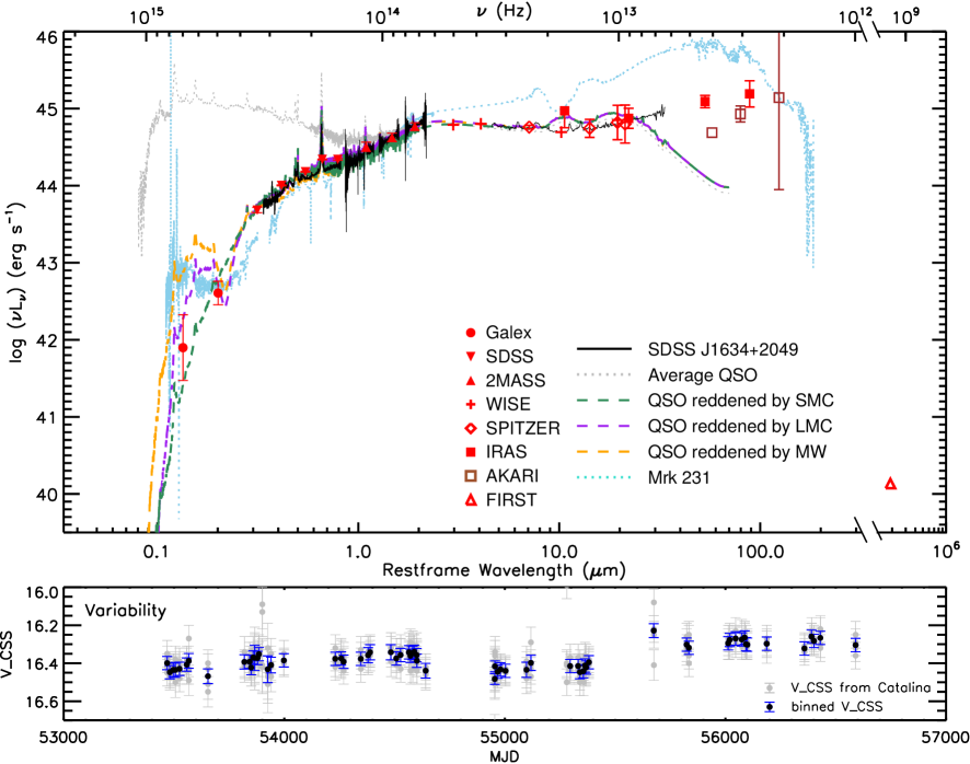
Figure 1.— Top: The broadband spectral energy distribution of J1634$+$2049 constructed from non-simultaneous photometry data (red) and spectra, corrected for Galactic reddening and brought to the restframe. The black solid lines are the SDSS spectrum, the NIR spectrum observed by P200 TripleSpec, and the $Spitzer$ IRS spectrum. Overplotted for comparison is the average QSO spectrum (gray dotted line; see the text); the reddened versions of the average QSO spectrum by different extinction curves are denoted by the orange (MW), purple (LMC), and green (SMC) dashed lines. The light blue doted line is the SED of Mrk 231 constructed from the multiband spectra scaled at $\sim 2\micron$. Bottom: the variability of the $V$ band of J1634$+$2049. The raw data (gray dots) are taken from Catalina Survey with the binned version within every day plotted also (black dot).

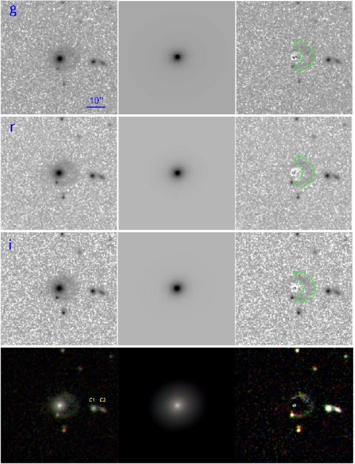
Figure 2.— SDSS images of J1634$+$2049 and the 2D imaging decomposition by GALFIT. From top to bottom are SDSS $g$, $r$, and $i$ bands, and the composite of the three bands, respectively. The left column shows the original image, the middle column shows the GALFIT model (PSF + Sérsic), and the right column shows the residual image. All images are oriented with north up and east to the left; the black line marks a scale of 10″($\sim$ 23.1 kpc). The green polygon denotes the ring region, which as well as the foreground stars has been masked out in GALFIT fitting.

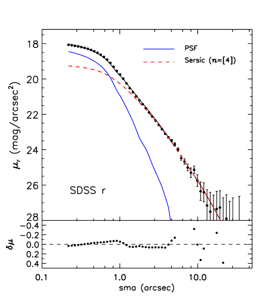
Figure 3.— Top: one-dimensional representation of the two-component GALFIT model applied to the SDSS $r$ image of J1634$+$2049: PSF for the nucleus (blue solid line) $n=4$ Sérsic function for the host galaxy (red dashed line). The sum of the two components is shown as the black solid line. The observed data are plotted as black dots with $\pm 1\sigma$ error bars. Bottom: the residuals between the observed data and the best-fit model.

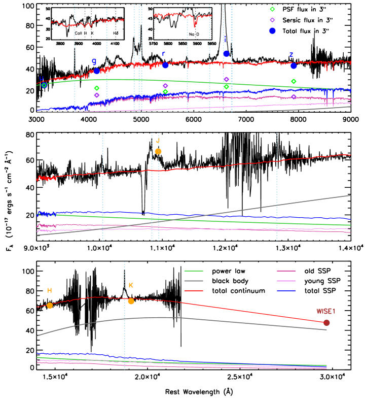
Figure 4.— Detailed decomposition for continuum of J1634$+$2049 in the rest frame wavelength range from 3000 Å to 3 $\micron$. The black solid line is the combined spectrum of SDSS (3350-8150 Å), DBSP (2900-9200 Å) and TripleSpec spectrum (8600 Å-2.2 $\micron$). The common part of the three spectra were weighted by spectral signal to noise ratio(S/N). The blue solid dots are fluxes of $u$, $g$, $r$, $i$, and $z$ bands in 3$\arcsec$ measured from SDSS images (see §2.3). The green and purple diamonds shows the decomposition of PSF and Sérsic components in 3 $\arcsec$ decomposed from SDSS images respectively. Orange and brown dots are the photometry fluxes from 2MASS $J$, $H$, $K$, and $WISE$ $W1$ bands. All the spectrum and photometry data are corrected for Galactic reddening and redshift. Green solid line represents the power-law component reddened by LMC extinction curve with $E_{\rm B-V}$ = 0.41, and the gray line represents the black body continuum from hot dust (torus) with a temperature of 1394 K. The magenta line shows the continuum of the old stellar population (age $\sim$ 9 Gyr), the violet line shows the heavily reddened continuum of the young stellar population (age $\sim$ 127 Myr; $E_{\rm B-V}$ = 2.2), and the blue solid line shows the sum flux of the old and the young stellar population.

Figure 5.— Demonstration of the profile of the various emission lines, particularly their blueshifted components (presumably caused by AGN outflow). Plotted are the observed spectra with continuum and Fe II emission subtracted (black lines), the total fitted profile of each emission line (red dashed lines), the sum of the unblueshifted components of each line (blue lines), the narrow blueshifted component (green lines), and broad blueshifted component (brown lines). The purple and olive dashed vertical lines indicate $-900$ $\mathrm{km~{}s^{-1}}$ and 0 $\mathrm{km~{}s^{-1}}$, respectively.

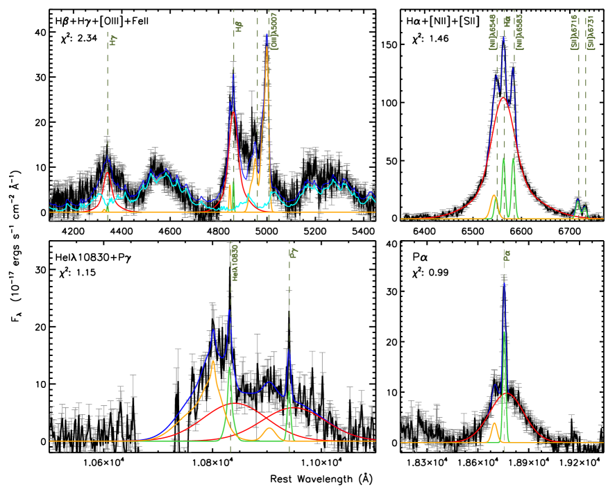
Figure 6.— The best-fit models for H$\beta$+ H$\gamma$+ [O III]+ FeII region (upper left), H$\alpha$+ [N II]+ [S II] region (upper right), He I$\lambda 10830$+P$\gamma$ region (lower left) and P$\alpha$ region (lower right). The blue solid line represents the total fit profile for each region. The red and green lines show the decomposed profiles of broad and narrow emission lines respectively. The orange line represents the blueshifted lines, and the cyan line represents optical Fe II multiplets.

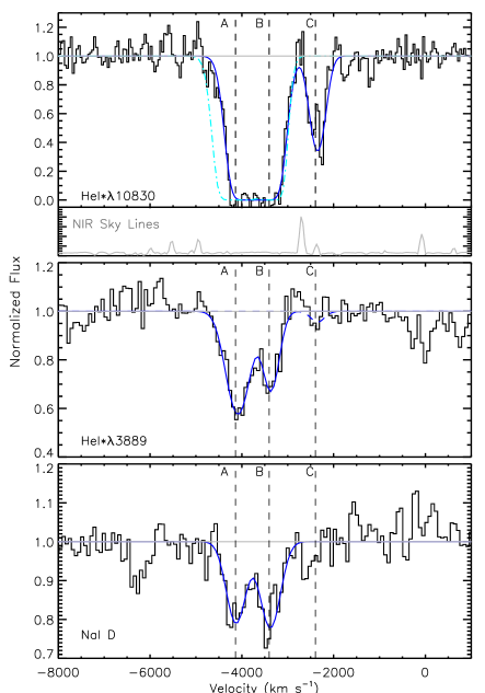
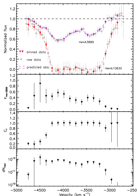
Figure 7.— Left: demonstration of the absorption troughs in He I*$\lambda\lambda 10830,3889$ and Na I D of J1634$+$2049, and the best fittings (in blue) by Voigt profile. The cyan lines in the upper panel show the predicted He I*$\lambda 10830$ profile derived from the He I*$\lambda 3889$ absorption line under the fully coverage assumption. Right: calculation results (top panel) of the He I* absorption lines of J1634$+$2049 using the partial-coverage model. The top panel shows the observed profiles (the gray dots) with $\pm 1\sigma$ error bars of He I*$\lambda\lambda 10830,3889$ the profiles binned by 3 pixels (the colored triangles) and the predicted profile from calculation (the dashed lines). The model parameters (the optical depth $\tau_{\rm He\,{\footnotesize I}*3889}$, covering fraction ($C_{\rm f}$), and column density ($dN_{\rm He\,{\footnotesize I}*}$) of the outflow) as a functions of velocity are shown in the other three panels.

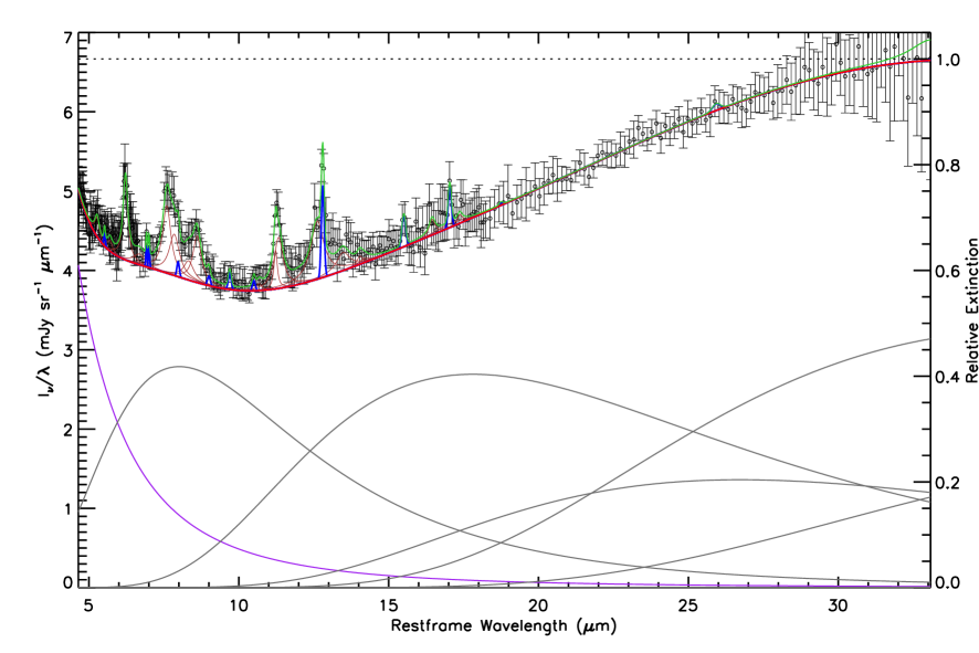
Figure 8.— Best-fit decomposition of J1634$+$2049 from 5 to 33 $\micron$ (rest frame) from PAHFIT. Details of the model parameters can be found in Smith et al. (2007). The black circles with error bars show the observed data. The gray lines represent the thermal dust continuum components, the purple line shows the stellar continuum, and the red line shows the total (dust + stellar) continuum. The brown lines represent the PAH features and the blue lines show the atomic and molecular lines. All components are diminished by the fully mixed extinction, indicated by the dotted black lines, with the axis at the right. The green line is the full fitted model, plotted over the observed flux intensities and uncertainties.

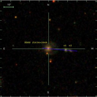
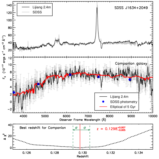
Figure 9.— Left: SDSS image of J1634$+$2049 and its companion galaxy, C1. The PA = 86° slit position is displayed by a blue line. Right: the upper panel shows the Lijiang 2.4m spectrum in the observer frame of J1634$+$2049 SDSS spectrum of J1634$+$2049 (gray line in upper panel) is displayed for a comparison. The middle panel displays the Lijiang 2.4m spectrum of the companion galaxy C1. SDSS photometry of C1 are also plotted on the observed spectrum as a check. The red line represents a template of an elliptical of 5 Gyr, which is obtained from (Polletta et al., 2007). The lower panel shows the $\Delta\chi^{2}$ of the grid search of the redshift of C1. The best redshift is $z=0.1298^{+0.007}_{-0.005}$.

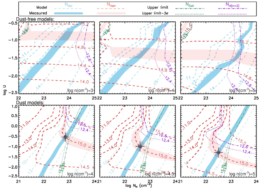
Figure 10.— Photoionization models of the absorption outflow in J1634$+$2049 assuming solar abundances. The upper three panels show results of the dust-free models, and the lower three panels show the models added the effects of dust grains mixed in the gas slab. Red and blue dashed lines represent the contours of ionic column densities of He I* and Na I, respectively. The red and blue shaded regions represent the locus of points ($N_{\rm H}$, $U$) able to reproduce the observed $N_{\rm He\,{\footnotesize I}*}$ and $N_{\rm Na\,{\footnotesize I}}$ with 1-$\sigma$ error respectively. The purple and the green dotted-dashed lines represent a upper limit on the ionic column densities of H($n$=2) and Ca II. Correspondingly, the purple and the green doted lines represent the upper limit minus 3 $\sigma$ error of H($n$=2) and Ca II, which indicate the confidence interval of the upper limit and also the decreasing direction of the ionic column density. The best models are marked by an open square with the systemic on the solution.

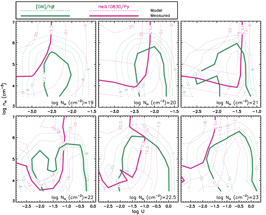
Figure 11.— Photoionization models of the emission line outflow in J1634$+$2049 assuming solar abundances and dust free. Different panels are for models with different $N_{\rm H}$. The green and violet dashed lines show the contours of line ratios of [O III]$\lambda 5007$/H$\beta$ and He I$\lambda 10830$/P$\gamma$ in ($U$, $n_{\rm H}$), respectively. The green and violet solid lines represent the locus of the measured upper limit for line ratios of [O III]$\lambda 5007$/H$\beta$ and He I$\lambda 10830$/P$\gamma$, respectively. The closed region surrounded by the green and the violet solid lines are the possible parameter space for the emission line outflow of J1634$+$2049.

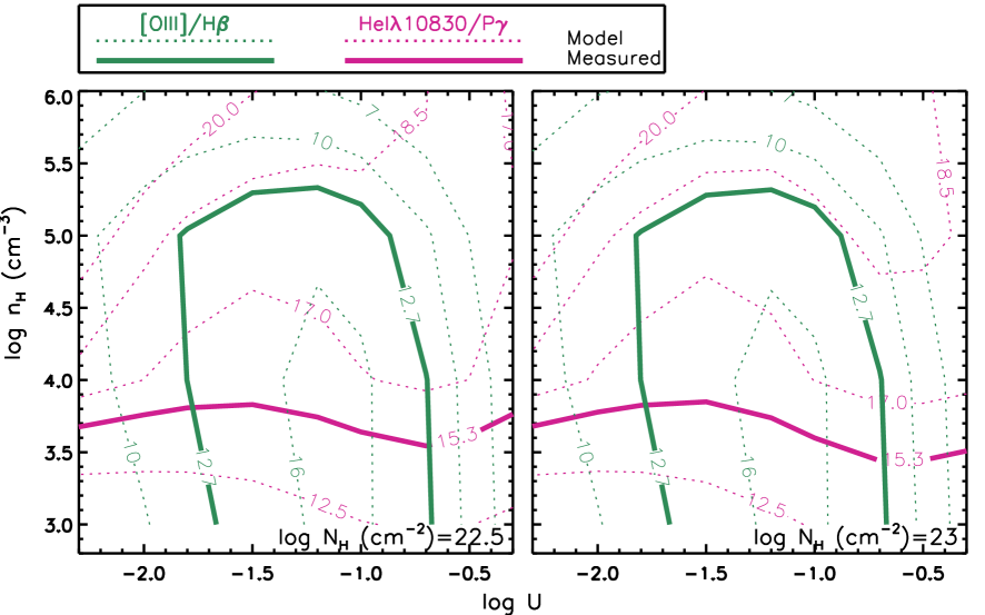
Figure 12.— Dust models of the emission line outflow in J1634$+$2049. The emission line ratios are directly extracted from the best dust models of absorption line outflow. The symbols are the same as Figure 11.

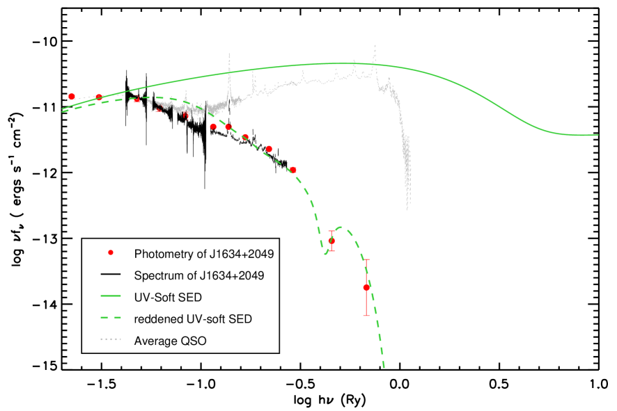
Figure 13.— Observed spectrum (the black solid lines) and photometry data (the red dots) of J1634$+$2049. The green solid curve represents the UV-soft SED scaled to the observed flux at the $WISEW1$ band. The green dashed curve shows the UV-soft SED reddened with the LMC extinction curve. The gray dotted line is the average QSO spectrum as shown in Figure 1.

Table 1Photometric Data

Band	Mag/Flux	Facility	Obs. Date	Reference
			(UT)
FUV	21.75$\pm$0.46 mag	$GALEX$	2006-12-23	1
NUV	20.47$\pm$0.17 mag	$GALEX$	2006-12-23	1
Petrosian $u$	18.94$\pm$0.04 mag	SDSS	2003-06-23	2, 3
Petrosian $g$	17.76$\pm$0.01 mag	SDSS	2003-06-23	2, 3
Petrosian $r$	16.95$\pm$0.01 mag	SDSS	2003-06-23	2, 3
Petrosian $i$	16.30$\pm$0.01 mag	SDSS	2003-06-23	2, 3
Petrosian $z$	16.07$\pm$0.01 mag	SDSS	2003-06-23	2, 3
$J$	14.65$\pm$0.04 mag	2MASS	1997-06-09	4
$H$	13.45$\pm$0.03 mag	2MASS	1997-06-09	4
$K_{s}$	12.25$\pm$0.03 mag	2MASS	1997-06-09	4
$W1$	10.73$\pm$0.02 mag	$WISE$	2010-05-29	5
$W2$	9.72$\pm$0.02 mag	$WISE$	2010-05-29	5
$W3$	7.07$\pm$0.02 mag	$WISE$	2010-02-21	5
$W4$	4.61$\pm$0.02 mag	$WISE$	2010-02-21	5
IRAC 8$\micron$	0.035$\pm$0.001 Jy	$Spitzer$	2008-04-30	6
$IRAS$ 12$\micron$	0.085$\pm$0.019 Jy	$IRAS$	1991-05-30	7
IRAC 16$\micron$	0.067$\pm$0.002 Jy	$Spitzer$	2008-04-30	6
IRS 22$\micron$	0.110$\pm$0.003 Jy	$Spitzer$	2008-04-30	6
MIPS 24$\micron$	0.114$\pm$0.003 Jy	$Spitzer$	2008-04-30	6
$IRAS$ 25$\micron$	0.141$\pm$0.018 Jy	$IRAS$	1991-06-06	7
$IRAS$ 60$\micron$	0.559$\pm$0.045 Jy	$IRAS$	1991-03-08	7
$AKARI$ 65$\micron$	0.239 Jy	$AKARI$	2011-09-08	8
$AKARI$ 90$\micron$	0.579$\pm$0.060 Jy	$AKARI$	2011-09-11	8
$IRAS$ 100$\micron$	1.172$\pm$0.199 Jy	$IRAS$	1991-04-11	7
$AKARI$ 140$\micron$	1.468$\pm$1.753 Jy	$AKARI$	2011-09-11	8
1.4 GHz	21.97$\pm$0.147 mJy	FIRST	1998-10-07	9

References. — (1)Morrissey et al. (2007) (2) York et al. (2000) (3)Abazajian et al. (2009) (4) Skrutskie et al. (2006) (5)Wright et al. (2010) (6) Houck et al. (2004) (7)Moshir et al. (1992) (8) Doi et al. (2009) (9) Becker et al. (1994)

Table 2GALFIT Decomposition

Band	Component	$m$	$M$	$m$ (in 3″)	$M$ (in 3″)	$n$	$r$(″/kpc)
SDSS $g$	PSF	18.68	-20.49	18.74	-20.43
	Sérsic	17.95	-21.22	19.13	-20.04	4	2.41/5.56
	Ring	19.85	-19.32
	C1	19.98	-19.15			3.32	0.55/1.26
SDSS $r$	PSF	18.16	-20.93	18.24	-20.85
	Sérsic	17.02	-22.07	17.99	-22.07	4	1.82/4.20
	Ring	18.91	-20.18
	C1	18.95	-20.10			2.46	0.49/1.13
SDSS $i$	PSF	17.51	-21.53	17.56	-21.48
	Sérsic	16.52	-22.52	17.29	-21.75	4	1.21/2.80
	Ring	18.43	-20.61
	C1	18.61	-20.40			2.34	0.45/1.03

Table 3Emission Line Parameters

Emission Line	Centroid	FWHM	Flux
	(Å)	($\mathrm{km~{}s^{-1}}$)	(10-17 erg s-1 cm-2)
[O II]$\lambda 3727$(narrow)	3727.39$\pm$0.21	491$\pm$5	184$\pm$3
[O II]$\lambda 3727$(outflow)	3720.19$\pm$2.22	738$\pm$5	89$\pm$8
H$\gamma$(broad)	4342.43	2955	487$\pm$25
H$\gamma$(narrow)	4340.74	343	8$\pm$5
H$\gamma$(outflow)	4327.58	737	7$\pm$9
H$\beta$(broad)	4863.52	2955	1378$\pm$14
H$\beta$(narrow)	4861.63	343	42$\pm$3
H$\beta$(outflow)	4846.50	737$\pm$20	58$\pm$5
[O III]$\lambda 5007$	4992.80$\pm$0.32	1707$\pm$18	1043$\pm$12
[O I]$\lambda 6300$	6299.87$\pm$0.53	421	61$\pm$6
H$\alpha$(broad)	6565.74$\pm$0.18	2955$\pm$12	8719$\pm$66
H$\alpha$(narrow)	6563.18$\pm$0.03	343$\pm$5	427$\pm$8
H$\alpha$(outflow)	6543.30$\pm$0.13	737	351$\pm$17
[N II]$\lambda 6583$	6583.05$\pm$0.03	370$\pm$4	458$\pm$6
[S II]$\lambda 6716$	6716.42$\pm$0.12	421$\pm$10	148$\pm$5
[S II]$\lambda 6731$	6730.80	421	106$\pm$4
He I$\lambda$10830(broad)	10840.33$\pm$1.48	3803	994$\pm$53
He I$\lambda$10830(narrow)	10831.33$\pm$0.45	178$\pm$12	162$\pm$25
He I$\lambda$10830(outflowN)	10801.14$\pm$0.33	140$\pm$23	21$\pm$7
He I$\lambda$10830(outflowB)	10782.34$\pm$0.33	1612$\pm$23	764$\pm$37
P$\gamma$(broad)	10948.39	3803	874$\pm$34
P$\gamma$(narrow)	10940.50$\pm$0.31	204$\pm$18	69$\pm$10
P$\gamma$(outflow)	10907.00	575	50$\pm$11
P$\alpha$(broad)	18768.64$\pm$0.20	3803$\pm$103	2484$\pm$79
P$\alpha$(narrow)	18755.96$\pm$0.19	310$\pm$11	486$\pm$13
P$\alpha$(outflow)	18697.69$\pm$1.64	575$\pm$75	146$\pm$16

Table 4Balmer Decrement

Decrement	Component	Value	$E_{\rm B-V}$
H$\alpha$/H$\beta$	broad	6.33$\pm$0.08	0.64$\pm$0.01
H$\alpha$/H$\beta$	narrow	10.17$\pm$0.75	1.05$\pm$0.06
H$\alpha$/H$\beta$	outflow (narrow)	6.05$\pm$0.60	0.60$\pm$0.09
P$\alpha$/H$\beta$	broad	1.80$\pm$0.06	0.66$\pm$0.01
P$\alpha$/H$\beta$	narrow	11.57$\pm$0.90	1.39$\pm$0.03
P$\alpha$/H$\beta$	outflow (narrow)	2.52$\pm$0.35	0.79$\pm$0.05

Table 5Recovered Dust Features and Line Strengths

Emission Line	Intensity	$EW$
	(10-20 W cm-2)	($\micron$)
PAH 6.2$\micron$	1.47$\pm$0.09	0.050$\pm$ 0.003
PAH 7.7$\micron$ complex	3.06$\pm$0.16	0.135$\pm$ 0.007
PAH 8.3$\micron$	0.57$\pm$0.12	0.028$\pm$ 0.006
PAH 8.6$\micron$	1.08$\pm$0.08	0.055$\pm$ 0.004
PAH 11.3$\micron$ complex	1.25$\pm$0.08	0.085$\pm$ 0.005
PAH 12.0$\micron$	0.10$\pm$0.09	0.007$\pm$ 0.006
PAH 12.6$\micron$ complex	1.44$\pm$0.14	0.106$\pm$ 0.010
PAH 13.6$\micron$	0.43$\pm$0.10	0.033$\pm$ 0.008
PAH 16.4$\micron$	0.13$\pm$0.07	0.011$\pm$ 0.006
PAH 17$\micron$ complex	0.34$\pm$0.25	0.029$\pm$ 0.019
[NeII]$\lambda 12.8\micron$	0.32$\pm$0.03	0.034$\pm$ 0.004
[NeIII]$\lambda 15.6\micron$	0.12$\pm$0.03	0.014$\pm$ 0.004

Table 6Physical Properties of the Outflow

log$n_{\rm H}$	log$N_{\rm H}$	log$U$	$v$	$R$	$\Omega$	log$L_{\rm Bol}$	$\dot{M}$	log$\dot{E}_{\rm k}$	$\dot{E}_{k}/L_{\rm Bol}$
(cm-3)	(cm-2)		$\mathrm{km~{}s^{-1}}$	(pc)	(%)	(ergs s-1)	($M_{\odot}$yr-1)	(ergs s-1)	(%)
4.0	22.85	-0.55	-3837	64.1	18.1 - 100	45.6	455–2513	45.3–46.0	49.2–272
4.5	22.6	-1.0	-3837	60.6	5.2 – 30.1	45.6	70–402	44.5–45.3	7.5–43.5
5.0	22.5	-1.3	-3837	48.1	3.0 – 17.4	45.6	25–147	44.1–44.8	2.8–15.9

References

- Abazajian et al. (2009) Abazajian, K. N., Adelman-McCarthy, J. K., Agüeros, M. A., et al. 2009, ApJS, 182, 543
- Acker et al. (1989) Acker, A., Köppen, J., Samland, M., & Stenholm, B. 1989, The Messenger, 58, 44
- Arav et al. (2001) Arav, N., Brotherton, M. S., Becker, R. H., et al. 2001, ApJ, 546, 140
- Baldwin et al. (1981) Baldwin, J. A., Phillips, M. M., & Terlevich, R. 1981, PASP, 93, 5
- Barvainis (1987) Barvainis, R. 1987, ApJ, 320, 537
- Becker et al. (1994) Becker, R. H., White, R. L., & Helfand, D. J. 1994, Astronomical Data Analysis Software and Systems III, 61, 165
- Bentz et al. (2009) Bentz, M. C., Peterson, B. M., Netzer, H., Pogge, R. W., & Vestergaard, M. 2009, ApJ, 697, 160
- Bertin & Arnouts (1996) Bertin, E., & Arnouts, S. 1996, A&AS, 117, 393
- Borguet et al. (2012) Borguet, B. C. J., Edmonds, D., Arav, N., Dunn, J., & Kriss, G. A. 2012, ApJ, 751, 107
- Bournaud & Combes (2003) Bournaud, F., & Combes, F. 2003, A&A, 401, 817
- Brauher et al. (2008) Brauher, J. R., Dale, D. A., & Helou, G. 2008, ApJS, 178, 280
- Bruzual & Charlot (2003) Bruzual, G., & Charlot, S. 2003, MNRAS, 344, 1000
- Burtscher et al. (2013) Burtscher, L., Meisenheimer, K., Tristram, K. R. W., et al. 2013, A&A, 558, A149
- Buta et al. (1999) Buta, R., Purcell, G. B., Cobb, M. L., et al. 1999, AJ, 117, 778
- Carswell et al. (1984) Carswell, R. F., Morton, D. C., Smith, M. G., et al. 1984, ApJ, 278, 486
- Cushing et al. (2004) Cushing, M. C., Vacca, W. D., & Rayner, J. T. 2004, PASP, 116, 362
- Condon et al. (1995) Condon, J. J., Anderson, E., & Broderick, J. J. 1995, AJ, 109, 2318
- Dimitrijević et al. (2007) Dimitrijević, M. S., Popović, L. Č., Kovačević, J., Dačić, M., & Ilić, D. 2007, MNRAS, 374, 1181
- Doi et al. (2009) Doi, Y., Etxaluze Azkonaga, M., White, G., et al. 2009, The Next-Generation Infrared Space Mission: SPICA, 4018
- Dong et al. (2005) Dong, X.-B., Zhou, H.-Y., Wang, T.-G., et al. 2005, ApJ, 620, 629
- Dong et al. (2008) Dong, X., Wang, T., Wang, J., et al. 2008, MNRAS, 383, 581
- Dunn et al. (2010) Dunn, J. P., Bautista, M., Arav, N., et al. 2010, ApJ, 709, 611
- Dong et al. (2011) Dong, X.-B., Wang, J.-G., Ho, L. C., et al. 2011, ApJ, 736, 86
- Dong et al. (2012) Dong, X.-B., Ho, L. C., Yuan, W., et al. 2012, ApJ, 755, 167
- Edelson & Malkan (1986) Edelson, R. A., & Malkan, M. A. 1986, ApJ, 308, 59
- Elvis et al. (1994) Elvis, M., Wilkes, B. J., McDowell, J. C., et al. 1994, ApJS, 95, 1
- Erwin et al. (2008) Erwin, P., Pohlen, M., & Beckman, J. E. 2008, AJ, 135, 20
- Farrah et al. (2007) Farrah, D., Bernard-Salas, J., Spoon, H. W. W., et al. 2007, ApJ, 667, 149
- Ferland et al. (1998) Ferland, G. J., Korista, K. T., Verner, D. A., et al. 1998, PASP, 110, 761
- Fitzpatrick (1999) Fitzpatrick, E. L. 1999, PASP, 111, 63
- Gaskell & Ferland (1984) Gaskell, C. M., & Ferland, G. J. 1984, PASP, 96, 393
- Glikman et al. (2006) Glikman, E., Helfand, D. J., & White, R. L. 2006, ApJ, 640, 579
- Greene & Ho (2005) Greene, J. E., & Ho, L. C. 2005, ApJ, 627, 721
- Greene & Ho (2005) Greene, J. E., & Ho, L. C. 2005, ApJ, 630, 122
- Greene & Ho (2007) Greene, J. E., & Ho, L. C. 2007, ApJ, 670, 92
- Gunn et al. (1998) Gunn, J. E., Carr, M., Rockosi, C., et al. 1998, AJ, 116, 3040
- Halpern & Steiner (1983) Halpern, J. P., & Steiner, J. E. 1983, ApJ, 269, L37
- Hjerting (1938) Hjerting, F. 1938, ApJ, 88, 508
- Hopkins et al. (2006) Hopkins, P. F., Hernquist, L., Cox, T. J., et al. 2006, ApJS, 163, 1
- Hopkins et al. (2008) Hopkins, P. F., Hernquist, L., Cox, T. J., & Kereš, D. 2008, ApJS, 175, 356
- Hopkins & Elvis (2010) Hopkins, P. F., & Elvis, M. 2010, MNRAS, 401, 7
- Houck et al. (2004) Houck, J. R., Roellig, T. L., van Cleve, J., et al. 2004, ApJS, 154, 18
- Into & Portinari (2013) Into, T., & Portinari, L. 2013, mnras, 430, 2715
- Ji et al. (2012) Ji, T., Wang, T.-G., Zhou, H.-Y., & Wang, H.-Y. 2012, Research in Astronomy and Astrophysics, 12, 369
- Ji et al. (2015) Ji, T., Zhou, H., Jiang, P., et al. 2015, ApJ, 800, 56
- Jiang et al. (2013) Jiang, N., Ho, L. C., Dong, X.-B., Yang, H., & Wang, J. 2013, ApJ, 770, 3
- Kauffmann et al. (2003) Kauffmann, G., Heckman, T. M., Tremonti, C., et al. 2003, MNRAS, 346, 1055
- Kawakatu et al. (2006) Kawakatu, N., Anabuki, N., Nagao, T., Umemura, M., & Nakagawa, T. 2006, ApJ, 637, 104
- Kennicutt (1998) Kennicutt, R. C., Jr. 1998, ARA&A, 36, 189
- Kewley et al. (2006) Kewley, L. J., Groves, B., Kauffmann, G., & Heckman, T. 2006, MNRAS, 372, 961
- Kim et al. (1995) Kim, D.-C., Sanders, D. B., Veilleux, S., Mazzarella, J. M., & Soifer, B. T. 1995, ApJS, 98, 129
- Komossa & Xu (2007) Komossa, S., & Xu, D. 2007, ApJ, 667, L33
- Kormendy & Ho (2013) Kormendy, J., & Ho, L. C. 2013, ARA&A, 51, 511
- Landt et al. (2008) Landt, H., Bentz, M. C., Ward, M. J., et al. 2008, ApJS, 174, 282
- Lebouteiller et al. (2011) Lebouteiller, V., Barry, D. J., Spoon, H. W. W., et al. 2011, ApJS, 196, 8
- Leighly et al. (2011) Leighly, K. M., Dietrich, M., & Barber, S. 2011, ApJ, 728, 94
- Leighly et al. (2014) Leighly, K. M., Terndrup, D. M., Baron, E., et al. 2014, ApJ, 788, 123
- Liu et al. (2015) Liu, W.-J., Zhou, H., Ji, T., et al. 2015, ApJS, 217, 11
- Lynds & Toomre (1976) Lynds, R., & Toomre, A. 1976, ApJ, 209, 382
- Mapelli et al. (2008) Mapelli, M., Moore, B., Ripamonti, E., et al. 2008, MNRAS, 383, 1223
- Mapelli & Mayer (2012) Mapelli, M., & Mayer, L. 2012, MNRAS, 420, 1158
- Markwardt (2009) Markwardt, C. B. 2009, Astronomical Data Analysis Software and Systems XVIII, 411, 251
- McConnell & Ma (2013) McConnell, N. J., & Ma, C.-P. 2013, ApJ, 764, 184
- Meyers & Peterson (1985) Meyers, K. A., & Peterson, B. M. 1985, PASP, 97, 734
- Misselt et al. (1999) Misselt, K. A., Clayton, G. C., & Gordon, K. D. 1999, ApJ, 515, 128
- Morrissey et al. (2007) Morrissey, P., Conrow, T., Barlow, T. A., et al. 2007, ApJS, 173, 682
- Moshir et al. (1992) Moshir, M., Kopman, G., & Conrow, T. A. O. 1992, Pasadena: Infrared Processing and Analysis Center, California Institute of Technology, 1992, edited by Moshir, M.; Kopman, G.; Conrow, T. a.o.,
- Netzer et al. (2007) Netzer, H., Lutz, D., Schweitzer, M., et al. 2007, ApJ, 666, 806
- Oke & Gunn (1982) Oke, J. B., & Gunn, J. E. 1982, PASP, 94, 586
- Pei (1992) Pei, Y. C. 1992, ApJ, 395, 130
- Peng et al. (2002) Peng, C. Y., Ho, L. C., Impey, C. D., & Rix, H.-W. 2002, AJ, 124, 266
- Peng et al. (2010) Peng, C. Y., Ho, L. C., Impey, C. D., & Rix, H.-W. 2010, AJ, 139, 2097
- Pohlen & Trujillo (2006) Pohlen, M., & Trujillo, I. 2006, A&A, 454, 759
- Polletta et al. (2007) Polletta, M., Tajer, M., Maraschi, L., et al. 2007, ApJ, 663, 81
- Rieke (1978) Rieke, G. H. 1978, ApJ, 226, 550
- Rieke et al. (2009) Rieke, G. H., Alonso-Herrero, A., Weiner, B. J., et al. 2009, ApJ, 692, 556
- Runnoe et al. (2012) Runnoe, J. C., Brotherton, M. S., & Shang, Z. 2012, mnras, 422, 478
- Sanders et al. (1988) Sanders, D. B., Soifer, B. T., Elias, J. H., et al. 1988, ApJ, 325, 74
- Sanders & Mirabel (1996) Sanders, D. B., & Mirabel, I. F. 1996, ARA&A, 34, 749
- Sérsic (1968) Sérsic, J. L. 1968, Cordoba, Argentina: Observatorio Astronomico, 1968,
- Scannapieco & Oh (2004) Scannapieco, E., & Oh, S. P. 2004, ApJ, 608, 62
- Schlegel et al. (1998) Schlegel, D. J., Finkbeiner, D. P., & Davis, M. 1998, ApJ, 500, 525
- Schweitzer et al. (2006) Schweitzer, M., Lutz, D., Sturm, E., et al. 2006, ApJ, 649, 79
- Skrutskie et al. (2006) Skrutskie, M. F., Cutri, R. M., Stiening, R., et al. 2006, AJ, 131, 1163
- Smith et al. (2007) Smith, J. D. T., Draine, B. T., Dale, D. A., et al. 2007, ApJ, 656, 770
- Smith et al. (2012) Smith, R., Lane, R. R., Conn, B. C., & Fellhauer, M. 2012, MNRAS, 423, 543
- Spoon et al. (2007) Spoon, H. W. W., Marshall, J. A., Houck, J. R., et al. 2007, ApJ, 654, L49
- Spoon et al. (2013) Spoon, H. W. W., Farrah, D., Lebouteiller, V., et al. 2013, ApJ, 775, 127
- Storey & Zeippen (2000) Storey, P. J., & Zeippen, C. J. 2000, MNRAS, 312, 813
- Theys & Spiegel (1976) Theys, J. C., & Spiegel, E. A. 1976, ApJ, 208, 650
- Theys & Spiegel (1977) Theys, J. C., & Spiegel, E. A. 1977, ApJ, 212, 616
- Toomre (1978) Toomre, A. 1978, Large Scale Structures in the Universe, 79, 109
- Wang et al. (2011) Wang, H., Wang, T., Zhou, H., et al. 2011, ApJ, 738, 85
- Weingartner & Draine (2001) Weingartner, J. C., & Draine, B. T. 2001, ApJ, 548, 296
- Werner et al. (2004) Werner, M. W., Roellig, T. L., Low, F. J., et al. 2004, ApJS, 154, 1
- Wright et al. (2010) Wright, E. L., Eisenhardt, P. R. M., Mainzer, A. K., et al. 2010, AJ, 140, 1868
- Wu & Jiang (2015) Wu, Y.-T., & Jiang, I.-G. 2015, ApJ, 805, 32
- Vacca et al. (2003) Vacca, W. D., Cushing, M. C., & Rayner, J. T. 2003, PASP, 115, 389
- Vanden Berk et al. (2001) Vanden Berk, D. E., Richards, G. T., Bauer, A., et al. 2001, AJ, 122, 549
- Veilleux et al. (2009) Veilleux, S., Rupke, D. S. N., Kim, D.-C., et al. 2009, ApJS, 182, 628
- Veilleux et al. (2013) Veilleux, S., Trippe, M., Hamann, F., et al. 2013, ApJ, 764, 15
- Véron et al. (2002) Véron, P., Gonçalves, A. C., & Véron-Cetty, M.-P. 2002, A&A, 384, 826
- Véron-Cetty et al. (2004) Véron-Cetty, M.-P., Joly, M., & Véron, P. 2004, A&A, 417, 515
- Xiao et al. (2011) Xiao, T., Barth, A. J., Greene, J. E., et al. 2011, ApJ, 739, 28
- York et al. (2000) York, D. G., Adelman, J., Anderson, J. E., Jr., et al. 2000, AJ, 120, 1579
- Zhang et al. (2011) Zhang, K., Dong, X.-B., Wang, T.-G., & Gaskell, C. M. 2011, ApJ, 737, 71
- Zhou et al. (2006) Zhou, H., Wang, T., Yuan, W., et al. 2006, ApJS, 166, 128