THE SIMPLEST POSSIBLE BOUNCING QUANTUM COSMOLOGICAL MODEL

Abstract

We present and expand the simplest possible quantum cosmological bouncing model already discussed in previous works: the trajectory formulation of quantum mechanics applied to cosmology (through the Wheeler-De Witt equation) in the FLRW minisuperspace without spatial curvature. The initial conditions that were previously assumed were such that the wave function would not change its functional form but instead provide a dynamics to its parameters. Here, we consider a more general situation, in practice consisting of modified Gaussian wave functions, aiming at obtaining a non singular bounce from a contracting phase. Whereas previous works consistently obtain very symmetric bounces, we find that it is possible to produce highly non symmetric solutions, and even cases for which multiple bounces naturally occur. We also introduce a means of treating the shear in this category of models by quantizing in the Bianchi I minisuperpace.

PACS Nos.: 98.80.Es, 98.80.-k, 98.80.Jk

1 Introduction

Although recent accumulation of data[2] seem to favor the standard[3] inflationary paradigm[4] with primordial perturbations originating from quantum vacuum fluctuations[5], a few riddles still need solutions, among which the presence of a primordial singularity[6]. It is often hoped, and shown explicitly in specific models, that quantum gravitational effects should take care of this problem, and indeed, many proposals have been made in this direction[7, 8, 9, 10], although not always successfully[11, 12].

Treating the Universe itself as a quantum object immediately raises the question of both the meaning of the wave function $\Psi$ and the issue of measurement. Indeed, whereas a tabletop experiment leads to a simple interpretation of $|\Psi|^{2}$ as the probability to measure whatever it is one wants to measure, when one is dealing with the wave function of the Universe, such an interpretation becomes instantly slightly more obscure. Moreover, what is it exactly that one measures in quantum cosmology that would collapse the wave function on the eigenvalue of? Such questions have been the subject of long debates, including possibilities to modify quantum mechanics itself by inclusion of non linear and stochastic terms in a new version of the Schrödinger equation.[13, 14]

Similarly using a quantum cosmological framework in which the usual quantum mechanics is modified, in Ref. AcaciodeBarros1998, a plausible solution to all questions and issues above was shown to possibly stem from assuming an actual (quantum) motion[15, 16, 17] of the scale factor $a$ for quantum cosmology expressed in the Friedmann-Lemaître-Robertson-Walker (FLRW) minisuperspace: quantizing a barotropic fluid along with the gravitational field, one obtains a well-defined time variable $T$ entitling to rewrite the Wheeler-De Witt equation in a Schrödinger form to which a de Broglie-Bohm (dBB) trajectory $a(T)$ can then assigned. With either dust or radiation, and with arbitrary spatial curvature, one sees that for a given initial (essentially gaussian) wave function, the resulting trajectory never goes through $a=0$, and hence that no singularity is ever reached: a bounce instead takes place.[20]

In what follows, we present an extension of this result aiming at generalizing the initial condition wave function $\Psi_{0}$ given at an arbitrary time: in the previous work[1], the initial wave functions that were used had been chosen in such a way that the only effect of the time evolution was to give a time dependency on the parameters without modifying their functional forms. For example, for a Gaussian initial condition, the time evolution just modifies the variance, adding a complex value to it. Here we assume more general initial wave packets for which this simple behavior does not hold.

To simplify matters, we restrict attention to flat spatial curvature (although in full generality this component should be included), but allow for the presence of shear and thus start with the Bianchi I Hamiltonian[22]. Splitting the wave function into a function of the scale factor only and a shear component eigenmode, we then reduce our system to the simplest possible case equivalent to the free particle, which we then endow with a complex initial wave function. Building the Hilbert space, we calculate the propagator and subsequently evolve this initial wave function to derive the necessary equation of motion of the scale factor. We then solve the dBB trajectory numerically to show that non symmetric bouncing solutions appear generic in this model. We conclude by discussing the generality of our result and providing the future investigation directions.

2 A Very Simple Hamiltonian

Our starting point will be the Hamiltonian, discussed in Ref. Bergeron:2015jpa, obtained to study the evolution of the anisotropic and compact locally flat spacetime with line element

$$\mathrm{d}s^{2}=-N^{2}(t)\mathrm{d}t^{2}+\sum_{i=1}^{3}a_{i}^{2}(t)\left(\mathrm{d}x^{i}\right)^{2},$$ (1)

and matter consisting in a radiation fluid with equation of state $w\equiv p/\rho=\frac{1}{3}$. In full generality, one could choose any value for $w$, leaving, as we will see below, the time parameter unfixed, but here we assume that we are considering extremely early stages of the Universe during which, if a fluid description is to make any sense at all (and that it questionable indeed), it will have to be a radiation fluid; setting $w=\frac{1}{3}$ is therefore, in our view, not restricting to a particular case but merely a physically motivated statement.

In the framework above, one sees that the relevant Hamiltonian provided by the gravitational part of the action (the fluid part is discussed in Sec. 3), assuming the conformal time choice $N\to a$ (and therefore $t\to\eta$ in what follows), reads

$$H=\frac{\Pi_{a}^{2}}{24}-\frac{p_{-}^{2}+p_{+}^{2}}{24a^{2}},$$ (2)

in terms of the canonical variables $a\equiv\left(a_{1}a_{2}a_{3}\right)^{\frac{1}{3}}$ (average scale factor) and its associated momentum $\Pi_{a}$, and the momenta $p_{-}$ and $p_{+}$, respectively conjugate of the shear-inducing variables $\beta_{-}\equiv\frac{1}{2\sqrt{3}}\ln\left(a_{1}/a_{2}\right)$ and $\beta_{+}\equiv\frac{1}{6}\ln\left(a_{1}a_{2}/a_{3}^{2}\right)$. Quantization is achieved by promoting these variables to operators in a Hilbert space (defined below) satisfying the usual canonical commutation relations $[\hat{a},\hat{\Pi}_{a}]=[\hat{\beta}_{\pm},\hat{p}_{\pm}]=i$ (we work in geometrical units in which $\hbar=c=G_{{}_{\mathrm{N}}}=1$).

2.1 Bianchi I

In order to move ahead, we first rescale the variables in such a way that they retain their commutation relations and thus perform the replacements $a\to\hat{a}/(2\sqrt{6})$ and $\Pi_{a}\to 2\sqrt{6}\hat{\Pi}_{a}$, leading to

$$\hat{H}=\hat{\Pi}_{a}^{2}-\left(\hat{p}_{-}^{2}+\hat{p}_{+}^{2}\right)\hat{a}^{-2},$$ (3)

which has to be compared with the usual FLRW case with no restriction on the spatial curvature $\mathcal{K}$ for which the last term is proportional to $\mathcal{K}\hat{a}^{2}$ (the difference, quartic in the scale factor, is the same that holds between the curvature and shear terms appearing in the classical Friedman equation in which the curvature terms is merely $\mathcal{K}/a^{2}$ while the shear energy density is $\propto a^{-6}$; see Ref. Battefeld:2014uga and references therein).

We now work in a mixed representation for the wave function in which the operators $\hat{a}$ and $\hat{p}_{\pm}$ are multiplication operators, their action on the wave function yielding mere multiplication by $c-$numbers, i.e., $\hat{a}\Psi=a\Psi$ and $\hat{p}_{\pm}\Psi=p_{\pm}\Psi$, so that the conjugate operators read $\hat{\Pi}_{a}=-i\partial/\partial a$ and $\hat{\beta}_{\pm}=i\partial/\partial p_{\pm}$; this is a position representation for the scale factor part and the momentum representation for the shear. Since the average scale factor $a$ is, by construction, a positive quantity, contrary to $p_{\pm}$ which are a priori arbitrary real numbers, the Hilbert space $\mathbb{H}$ is contained in the set of square integrable functions of $\mathbb{R}^{+}$ and $\mathbb{R}^{2}$, namely

$$\mathbb{H}\subset\Set{f\left(a,p_{+},p_{-}\right)\in\mathbb{C}}{\int_{0}^{\infty}\mathrm{d}a\int_{-\infty}^{\infty}\mathrm{d}p_{+}\int_{-\infty}^{\infty}\mathrm{d}p_{-}|f\left(a,p_{+},p_{-}\right)|^{2}<\infty}.$$ (4)

The eigenvalue equation $\hat{H}\Psi=\ell^{2}\Psi$ (we note $\ell^{2}$ the eigenvalue of the Hamiltonian operator for later convenience) then transforms into

$$-\frac{\partial^{2}\mathcal{U}^{(k)}_{\ell}}{\partial a^{2}}-\frac{k^{2}}{4a^{2}}\mathcal{U}^{(k)}_{\ell}=\ell^{2}\mathcal{U}^{(k)}_{\ell},$$ (5)

where we set $k^{2}\equiv 4(p_{+}^{2}+p_{-}^{2})$ and we have expanded the total wave function in terms of the eigenstates $\chi(\beta_{\pm})$ of $\hat{\beta}_{\pm}$, i.e. $\chi\propto\exp[i(p_{+}\beta_{+}+p_{-}\beta_{-})]$, as

$$\Psi\left(a,p_{\pm}\right)=\int_{0}^{\infty}\mathrm{d}\ell\int_{-\infty}^{\infty}\mathrm{d}\beta_{+}\int_{-\infty}^{\infty}\mathrm{d}\beta_{-}\tilde{\Psi}\left(\ell,\beta_{\pm}\right)\mathrm{e}^{i[\beta_{+}p_{+}+\beta_{-}p_{-}]}\mathcal{U}^{(k)}_{\ell}(a).$$ (6)

Our Hilbert space will then be completed by obtaining the solutions for the energy eigenmodes $\mathcal{U}^{(k)}_{\ell}(a)$.

2.2 Hilbert space and boundary conditions

We now implement the requirement that the Hamiltonian should be self-adjoint, namely that

$$\int\mathrm{d}a\,\mathrm{d}^{2}p\,\left(H\Psi\right)^{*}\Psi=\int\mathrm{d}a\,\mathrm{d}^{2}p\,\Psi^{*}\left(H\Psi\right),$$ (7)

with the limits of integration defined in (4). As already mentioned above, the set of normalizable functions is too large and the actual Hilbert space $\mathbb{H}$ must be restricted to those normalizable functions such that the condition above is satisfied. We note that the condition (7) is automatically satisfied if the Hamiltonian eigenvectors form an orthonormal basis, i.e.

$$\int_{0}^{\infty}\mathrm{d}a\,\mathcal{U}^{(k)*}_{\ell}(a)\mathcal{U}^{(k)}_{\ell^{\prime}}(a)=\delta(\ell-\ell^{\prime})$$ (8)

and

$$\int_{0}^{\infty}\mathrm{d}\ell\int_{-\infty}^{\infty}\mathrm{d}\beta_{+}\int_{-\infty}^{\infty}\mathrm{d}\beta_{-}|\tilde{\Psi}\left(\ell,\beta_{\pm}\right)|^{2}\ell^{2}<\infty.$$ (9)

We therefore define our Hilbert space $\mathbb{H}$ to be the set of square integrable functions of the form (6) where the basis is orthonormal in the sense of (8) and the functions $\tilde{\Psi}\left(\ell,\beta_{\pm}\right)$ satisfy Eq. (9).

Setting $\nu=\frac{1}{2}\sqrt{1-k^{2}}$, we obtain the general solution for the energy eigenmodes

$$\mathcal{U}^{(k)}_{\ell}(a)=c_{+}\sqrt{a\ell}J_{\nu}(a\ell)+c_{-}\sqrt{a\ell}J_{-\nu}(a\ell),$$ (10)

in terms of the Bessel functions $J_{\nu}$, with $c_{\pm}$ complex numbers satisfying $|c_{+}|^{2}+|c_{-}|^{2}=1$. Imposing the condition (8) then demands that either $c_{+}$ or $c_{-}$ vanishes. Apart from an irrelevant phase factor, one can therefore, without lack of generality, set $c_{+}=1$ and $c_{-}=0$, or the opposite $c_{+}=0$ and $c_{-}=1$; given the initial wave function choice, this will lead to impose different boundary conditions.

3 Time Evolution

As alluded to in the introduction, the existence of a fluid implies that of a preferred time slicing, and hence of a natural time parameter $t$ for the Schrödinger equation. Following Schutz formalism[18, 19], the velocity potential of the fluid allows to define a field whose properties are similar to that expected for a time variable. One then needs to fix the coordinate time variable appearing in (1) through a clever choice of the lapse function $N(t)$ adapted to the fluid. The most appropriate choice in (1) happens to depend on the equation of state of the fluid, and for a radiation dominated universe, one can set $N=a$, so the relevant time is the usual conformal time $\eta$, in terms of which the fluid canonical momentum reads $\hat{P}_{\mathrm{fluid}}=-i\partial_{\eta}$. This momentum enters the Hamiltonian linearly, so that the Wheeler-De Witt equation reads like a simple Schödinger equation, resulting in an evolution operator $U(\eta,\eta_{0})$ satisfying

$$i\frac{\partial U}{\partial\eta}=\hat{H}U\ \ \ \ \Longrightarrow\ \ \ \ \ U(\eta,\eta_{0})=\mathrm{e}^{-i\left(\eta-\eta_{0}\right)\hat{H}},$$ (11)

with $\eta_{0}$ an arbitrary initial time. Anticipating on the dBB trajectory, we note that, contrary to previous works, we do not intend here to impose initial condition at the expected bounce time at which $\mathrm{d}a/\mathrm{d}\eta=0$, assuming such a time to exist, but we will instead demand arbitrary initial condition in a contracting stage $\mathrm{d}a/\mathrm{d}\eta<0$ and actually evolve the universe until it bounces (again anticipating that it will do so).

3.1 Propagator

Our ultimate goal is, starting from an arbitrary initial wave function $\Psi_{0}(a)=\Psi(a;\eta_{0})$, to follow its time development $\Psi(a;\eta)$, whose phase $S(a;\eta)$ provides the dBB trajectory through

$$\frac{\mathrm{d}a}{\mathrm{d}\eta}=\frac{\partial S}{\partial a}=\frac{i}{2|\Psi|^{2}}\left(\Psi\frac{\partial\Psi^{*}}{\partial a}-\frac{\partial\Psi}{\partial a}\Psi^{*}\right),$$ (12)

and to figure under which conditions this time evolution, starting from a contracting scale factor, leads to a regular bouncing solution. We shall deal with the initial condition in the forthcoming section, and for now on concentrate on the propagator $G(a,p_{\pm},a_{0},p^{0}_{\pm})\equiv\langle a,p_{\pm}|U|a_{0},p^{0}_{\pm}\rangle$ evolving the state $|a_{0},p^{0}_{\pm}\rangle$ at time $\eta_{0}$ into $|a,p_{\pm}\rangle$ at time $\eta$.

In order to obtain this propagator, we first express the time evolution operator on the Fourier modes as

$$U=\int\mathrm{d}^{2}\beta\!\int_{0}^{\infty}\!\mathrm{d}\ell\,U(\eta,\eta_{0})|\ell,\beta_{\pm}\rangle\langle\ell,\beta_{\pm}|=\int\mathrm{d}^{2}\beta\!\int_{0}^{\infty}\!\mathrm{d}\ell\,\mathrm{e}^{-i\ell^{2}\Delta\eta}|\ell,\beta_{\pm}\rangle\langle\ell,\beta_{\pm}|,$$ (13)

with $\Delta\eta\equiv\eta-\eta_{0}$. This leads to

$$G(a,p_{\pm},a_{0},p^{0}_{\pm})=\delta^{(2)}(p_{\pm}-p^{\prime}_{\pm})\int_{0}^{\infty}\!\mathrm{d}\ell\,\mathrm{e}^{-i\ell^{2}\Delta\eta}\mathcal{U}_{\ell}^{(k)}(a)\mathcal{U}_{\ell}^{(k)*}(a^{\prime}),$$ (14)

where we have used $\langle a,p_{\pm}|\ell,\beta_{\pm}\rangle=\mathcal{U}_{\ell}^{(k)}(a)\exp[-i(p_{+}\beta_{+}+p_{-}\beta_{-})]/(2\pi)$. As expected, we see that if one starts with an eigenstate of $\hat{p}_{\pm}$, the subsequent time evolution remains on this state. From now on, we shall therefore discard the shear contribution insofar as it does not contribute to the equation of motion and merely assume the value of the shear to be fixed; we therefore simply denote the propagator by $G(a,a_{0};\eta)$ in what follows.

The propagator (14) needs be regularized, which is done by replacing $\Delta\eta$ by $\widetilde{\Delta\eta}=\Delta\eta(1+i\epsilon)$, with $\epsilon\ll 1$. Then, using Eq. (10.22.67) of Ref. Olver:2010:NHMF, one finds

$$G(a,a_{0};\eta)=-\frac{i\sqrt{aa_{0}}}{2\widetilde{\Delta\eta}}\mathrm{e}^{\frac{i}{4}(a^{2}+a_{0}^{2})/\widetilde{\Delta\eta}-i\alpha\pi/2}J_{\nu}\left(\frac{aa_{0}}{2\widetilde{\Delta\eta}}\right),$$ (15)

thanks to which we are now in a position to derive the wave function at an arbitrary time.

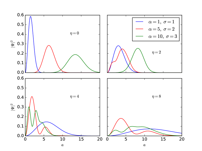
Figure 1: Initial wave function and its time evolution for various values of the localization $\alpha$ and spread $\sigma$. We used $\mathcal{H}_{\mathrm{ini}}=-0.1$ for all wave functions and $\nu=\frac{1}{2}$, sticking to the FLRW case to evolve the wave functions. As expected, the wave form changes dramatically during the time evolution, as in particular the mode, depending on its initial localization and spread, eventually reaches the potential wall at $a=0$ at which point the wave function bounces off. Oscillations then appear, due to the reflection on the wall, inducing a significant change in the subsequent time evolution; these changes are responsible, as we show below, for the completely new behavior of the scale factor exhibited on Fig. 2

3.2 Wave function

Having set the general framework for Bianchi I, we now simplify once more the model to restrict attention to the flat FLRW case, which represents a subset of Bianchi I; the complete analysis of the Bianchi I case will be presented elsewhere in a future work[24]. As we discuss below, the wave function proposed in Ref. AcaciodeBarros1998 can be generalized to yield new bouncing solutions. We shall accordingly consider an initial wave function at time $\eta_{0}$ which we demand to be localized around a certain initial value $a_{\mathrm{ini}}$ of the scale factor and having a complex phase in order to account for a possible initial velocity. Generalizing Ref. AcaciodeBarros1998, we set the normalized form

$$\Psi_{0}(a)=\langle a,p_{\pm}|\Psi_{0}\rangle=\frac{2^{(1-2\alpha)/4}\ a^{\alpha}}{\sigma^{\alpha+1/2}\sqrt{\Gamma\left(\alpha+\frac{1}{2}\right)}}\exp\left[-\frac{1}{2}a^{2}\left(\frac{1}{2\sigma^{2}}-i\mathcal{H}_{\mathrm{ini}}\right)\right],$$ (16)

where $\alpha$, $\sigma$ and $\gamma$ are real but otherwise arbitrary parameters. The wave function (16) peaks at $a_{\mathrm{ini}}=\sqrt{2\alpha}\sigma$ (maximum of $|\Psi_{0}|^{2}$), has a mean value at $\bar{a}=\langle a\rangle=\sqrt{2}\sigma\Gamma\left(1+\alpha\right)/\Gamma\left(\frac{1}{2}+\alpha\right)$ and variance $\langle\left(a-\bar{a}\right)^{2}\rangle=\sigma^{2}\left[1+2\alpha-2\Gamma^{2}\left(1+\alpha\right)/\Gamma^{2}\left(\frac{1}{2}+\alpha\right)\right]$. As shown on Fig. 1, the peak localization is essentially given by $\alpha$ while the spread mostly stems from the value of $\sigma$. Finally, applying (12) to the initial $\Psi_{0}$ (16), one finds that the coefficient $\mathcal{H}_{\mathrm{ini}}$ actually represents the initial value of the conformal Hubble parameter, hence the name of the parameter.

Equipped with the initial wave function (16) and the propagator (15), we are now in position to derive the equation of motion for the dBB scale factor. The wave function at time $\eta$ is

$$\Psi(a;\eta)=\langle a|U(\eta,\eta_{0})|\Psi_{0}\rangle\propto\int_{0}^{\infty}\!\mathrm{d}b\,\sqrt{ab}\mathrm{e}^{\frac{i}{4}(a^{2}+b^{2})/\widetilde{\Delta\eta}}J_{\nu}\!\left(\frac{ab}{2\widetilde{\Delta\eta}}\right)b^{\alpha}\mathrm{e}^{-\frac{1}{2}b^{2}\left(\frac{1}{2\sigma^{2}}-i\mathcal{H}_{\mathrm{ini}}\right)},$$ (17)

which, although it happens to be explicitly integrable in terms of hypergeometric functions, is not particularly illuminating. Figure 1 also shows the typical time evolution (17) for the modulus of the wave function. This evolution clearly differs from that of Ref. AcaciodeBarros1998 where it would hold its analytical shape at all times with time-dependent parameters. Here, one sees that the boundary condition at $a=0$ acts as an infinite potential wall such that, when the wave function evolves towards it, it bounces off, thereby inducing subsequent oscillations that can change dramatically the dBB trajectories, as we now discuss.

4 Results: from Bianchi I to FLRW

Let us move on to the results, and for the purpose of exemplifying, concentrate on the shearless limit whereby $\nu\to\frac{1}{2}$. The full analysis of the Bianchi I case will be provided elsewhere[24], and for the purpose of this work, we will make contact with Ref. AcaciodeBarros1998 by going to the vanishing shear limit for which $k=0$, and hence $\nu=\frac{1}{2}$, so the basis simplifies to mere sines and cosines. In Ref. AcaciodeBarros1998, the requirement that $\hat{H}$ be self-adjoint was shown to lead to the condition

$$\lim_{a\to 0}\frac{\mathrm{d}\Psi(a)}{\mathrm{d}a}=\lim_{a\to 0}\alpha_{\mathrm{BC}}\Psi(a),$$ (18)

with $\alpha_{\mathrm{BC}}\in(-\infty,\infty)$. The cases studied then correspond respectively to $\alpha_{\mathrm{BC}}\to 0\Longrightarrow(c_{-}=1,c_{+}=0)$ and $\alpha_{\mathrm{BC}}\to\infty\Longrightarrow(c_{-}=0,c_{+}=1)$, as already mentioned. The Hamiltonian reduces to that of a free particle on the half-line with the point $a=0$ equivalent to an infinite potential wall. In our final result (17), the Bessel function then reduces to a hyperbolic sine of its argument, so that most calculations are analytically tractable. We shall not go along this direction here[24] and instead concentrate on a numerical evaluation of the dBB trajectories, comparing those with previous calculations.

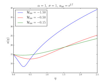
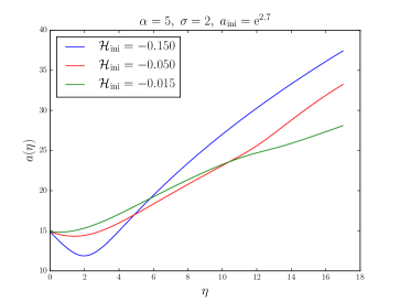
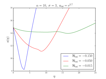
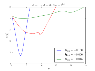
Figure 2: Illustration, for the shearless case $\nu=\frac{1}{2}$, of typical bouncing models obtained as solutions of the dBB equation of motion for the scale factor. The curves are labeled with the initial condition assumed for $\mathcal{H}_{\mathrm{ini}}$, and the solutions are obtained for values of $\alpha$ and $\sigma$ as in Fig. 1. One clearly sees that not only are such bouncing solutions not necessarily symmetric in time, but also that they can produce many bounces and not just one, even in the oversimplified situation of the flat shearless FLRW.

The pioneering solutions obtained in Ref. AcaciodeBarros1998 for the shearless case with no spatial curvature depend on two parameters, denoted $\eta_{*}$ and $a_{\mathrm{B}}$, and read

$$a(\eta)=a_{\mathrm{B}}\sqrt{1+\left(\frac{\eta}{\eta_{*}}\right)^{2}};$$ (19)

these parameters can be understood respectively as the typical bounce duration ($\eta_{*}$) and the minimum value of the scale factor ($a_{\mathrm{B}}$). This family of solution has very simple properties: first, as expected from a quantum gravity framework, they solve the singularity problem (what would be the point to have a quantum gravity model with singularities?) in the sense that the contracting phase never reaches the singular point $a=0$ since the minimum scale factor $a_{\mathrm{B}}>0$ unless one sets $a_{\mathrm{B}}=0$ in the first place, in which case the solution is singular at all times and thus lacks any physical relevance.

A second conclusion that can be drawn from (19) is that there is one and only one bounce taking place, with a regular decrease of the scale factor followed by a simple bounce and a subsequent regular increase. In a sense, this is the simplest extension of the standard cosmological model that can be thought of. Finally, and this is possibly the most crucial point, the bounces induced by (19) are all symmetric in time.

Figure 2 shows various solutions assuming different values for the initial scale factor and conformal Hubble parameter, for the cases depicted on Fig. 1. It is apparent that the very simple solution of Ref. AcaciodeBarros1998, is merely an exceptional case. In the cases studied here, we find that not only is the bounce often non symmetric in time, but also that many bounces can naturally occur, and in a way which is quite sensitive to the initial condition one sets on $a_{\mathrm{ini}}$ and $\mathcal{H}_{\mathrm{ini}}$.

Our study opens a wide range of new studies that need now be done for a complete understanding of such bouncing scenarios. First, the case with non vanishing shear must be investigated in details, with particular emphasis on the so-called BKL instability (see again Ref. Battefeld:2014uga for a thorough discussion of bounce models and their problems) according to which a pre-existing shear can spontaneously lead to many new Kasner-like singularities.

The second point that should be examined in details concerns the propagation of perturbations through such a complicated bounce. In models such as those based on dBB trajectories, it was found that perturbations can be easily evaluated in a way reminiscent the ordinary perturbation theory based on general relativity, but with the scale factor replaced by that obtained along the dBB trajectory[25, 26, 27]. With characteristic solutions exhibiting such features as shown on Fig. 2, it is clear that the potential for the perturbations will have many new interesting consequences that we hope to clarify in a further extension of the current work.

References

- [1] J. Acacio de Barros, N. Pinto-Neto and M. A. Sagioro-Leal, Phys. Lett. A 241, 229 (1998).
- [2] Planck Collaboration, N. Aghanim et al., arXiv:1507.02704 [astro-ph.CO].
- [3] P. Peter and J.-P. Uzan, Primordial Cosmology (Oxford University Press, 2009).
- [4] J. Martin, C. Ringeval and V. Vennin, Physics of the Dark Universe 5, 75 (2014).
- [5] V. F. Mukhanov, H. A. Feldman and R. H. Brandenberger, Phys. Rep. 215, 203 (1992).
- [6] A. Borde, A. H. Guth and A. Vilenkin, Phys. Rev. Lett. 90, 151301 (2003).
- [7] M. Gasperini and G. Veneziano, Astropart. Phys. 1, 317 (1993).
- [8] R. H. Brandenberger, String Gas Cosmology, in String Cosmology, J.Erdmenger (Ed.), Wiley, p. 193 (2008).
- [9] J. Khoury, B. A. Ovrut, P. J. Steinhardt and N. Turok, Phys. Rev. D64, 123522 (2001).
- [10] M. Fanuel and S. Zonetti, Europhys. Lett. 101, 10001 (2013).
- [11] R. Kallosh, L. Kofman and A. D. Linde, Phys. Rev. D64, 123523 (2001).
- [12] J. Martin, P. Peter, N. Pinto-Neto and D. J. Schwarz, Phys. Rev. D65, 123513 (2002).
- [13] J. Martin, V. Vennin and P. Peter, Phys. Rev. D86, 103524 (2012).
- [14] G. León and D. Sudarsky, JCAP 1506, 020 (2015).
- [15] L. de Broglie, J. Phys. Radium 8, 225 (1927).
- [16] D. Bohm, Phys. Rev. 85, 166 (1952).
- [17] P. Holland, The quantum theory of motion (CUP, Cambridge, England, 1993).
- [18] B. F. Schutz, Phys. Rev. D2, 2762 (1970).
- [19] B. F. Schutz, Phys. Rev. D4, 3559 (1971).
- [20] D. Battefeld and P. Peter, Phys. Rept. 571, 1 (2015).
- [21] N. Pinto-Neto, Phys. Rev. D79, 083514 (2009).
- [22] H. Bergeron, A. Dapor, J. P. Gazeau and P. Małkiewicz, Phys. Rev. D91, 124002 (2015), [Addendum: Phys. Rev. D91, 129905 (2015)].
- [23] F. W. J. Olver, D. W. Lozier, R. F. Boisvert and C. W. Clark (eds.), NIST Handbook of Mathematical Functions (Cambridge University Press, New York, NY, 2010). Print companion to Ref. \refciteNIST:DLMF.
- [24] P. Peter and S. D. P. Vitenti, in preparation (2016).
- [25] P. Peter, E. Pinho and N. Pinto-Neto, JCAP 7, 14 (2005).
- [26] E. J. C. Pinho and N. Pinto-Neto, Phys. Rev. D76, 023506 (2007).
- [27] P. Peter, E. J. C. Pinho and N. Pinto-Neto, Phys. Rev. D75, 023516 (2007).
- [28] NIST Digital Library of Mathematical Functions http://dlmf.nist.gov/, Release 1.0.10 of 2015-08-07, Online companion to Ref. \refciteOlver:2010:NHMF.