Evolution to the Quark-Gluon Plasma

Abstract

Theoretical studies on the early-time dynamics in the ultra-relativistic heavy-ion collisions are reviewed including pedagogical introductions on the initial condition with small-$\mathrm{x}$ gluons treated as a color glass condensate, the bottom-up thermalization scenario, plasma/glasma instabilities, basics of some formulations such as the kinetic equations and the classical statistical simulation. More detailed discussions follow to make an overview of recent developments on the fast isotropization, the onset of hydrodynamics, and the transient behavior of momentum spectral cascades.

1 Introduction

Early thermalization is the last and greatest unsolved problem in the ultra-relativistic heavy-ion collisions that have aimed to create a new state of matter out of quarks and gluons, i.e. a state called Quark-Gluon Plasma (QGP). As a consequence of non-perturbative and non-linear nature of the “strong interaction”, quarks and gluons and any colored excitations in general cannot be detected directly in laboratory experiments, which is an intuitive description of the color confinement phenomenon: quarks and gluons must be confined into color-singlet hadrons such as mesons and baryons. If the temperature $T$ is comparable to the typical scale of the strong interaction, i.e. $\Lambda_{\rm QCD}\sim 0.2\,\mbox{GeV}$ ($\sim 2\times 10^{12}\,\mbox{K}$), however, fundamental degrees of freedom should become more relevant and we may be able to probe some properties of hot and dense matter with quarks and gluons manifested. Then, such ambitious dreams to create a QGP by our hands have motivated the installation of high-energetic beams (see an essay [1] about two decades from dreams to beams). In fact, an extraordinarily high-energetic collision of two nuclei is a unique tool to realize such high energy density and temperature. It is widely believed that our wish to create the QGP has been successfully granted at Relativistic Heavy-Ion Collider (RHIC) and more activities at even higher energies are continued to Large Hadron Collider (LHC). There are, however, still some disputes about physical characteristics of the QGP from the theoretical point of view. All subtleties come from lack of clear-cut definition of the QGP from the first-principle theory of the strong interaction, i.e. quantum chromodynamics (QCD).

Perturbative calculations based on QCD have been established as theoretical descriptions in terms of quasi-particles of quarks and gluons (or “partons” collectively). Although there is no order parameter for a change from the hadronic phase to the partonic phase, we may well give a working definition of the QGP as a state that satisfies following (at least) two conditions. First, the physical degrees of freedom should be partons rather than hadrons, so that perturbative QCD (pQCD) can be a good description of the system. Second, the created state should form matter unlike a simple superposition of each partonic reaction. For this latter condition, for decades conventionally, a far stronger condition of thermalization had been imposed. Precisely speaking, local thermal equilibrium (LTE) had been assumed to link theoretical modeling to experimental QGP signatures. It is, however, very hard to account for the LTE with QCD microscopic processes within a time scale $\lesssim\Lambda_{\rm QCD}^{-1}\sim 1\,\mbox{fm}/c$. Eventually, after many trials and errors (one of earliest discussions can be found in [2] and the difficulty was revisited in [3]), theoretical ideas went around came around to the very starting point – what is matter at all? This issue is sometimes discussed in the context of the origin of collectivity of smaller systems involving proton, deutron, and light ions at LHC energies.

In this review, we do not discuss experimental and phenomenological studies of collectivity in small systems, which are currently ongoing, and we still need wait to see an ordered consensus out from disordered arguments. Here, we would look over purely theoretical approaches to reveal real-time QCD dynamics during the evolution to the QGP.  Fortunately, we can specify the trustworthy initial condition for the system right after the heavy-ion collisions using our pQCD knowledge. It is known that the gluon distribution function has increasing behavior with increasing reaction energy and classical color fields give a better description of such an overpopulated state than individual gluons, which can be understood in analogy to Weizsäcker-Williams fields in quantum electrodynamics (QED). The theoretical framework with coherent classical color fields (sometimes called non-Abelian Weizsäcker-Williams fields [4]) is known as the color glass condensate (CGC). Thus, we can say that, for a full understanding of the QGP physics, the missing link is a bridge between the CGC initial condition and the QGP described well by hydrodynamic equations. In other words, using a more general term, we can define our theoretical question as follows: How can a full quantum system get to a LTE state as a solution of the initial value problem starting with coherent fields?

Limiting our considerations to a specific situation in the relativistic heavy-ion collision, we can categorize the issues of thermalization into three distinct (and probably related) characterizations — isotropization, hydrodynamization, and spectral cascades. Let us briefly address them in order. The first is the (partial) isotropization. In the case of the heavy-ion collision, the system is expanding in time and the interaction should be turned off for a dilute system as long as we can neglect running effects of the strong coupling constant or confining forces. Such a theoretically idealized limit of non-interacting quarks and gluons in an expanding box is often called the free-streaming limit. The isotropization problem is an issue of how to explain the fact that the system can resist against a tendency falling into the free-streaming limit especially when the system is expanding. The second is the onset where hydrodynamic equations start working well to capture the real-time evolution of the system. In some literature this onset is discussed under the name of the hydronization or hydrodynamization. If the system sits in the LTE state, the hydrodynamic model should be valid, and in this sense, the LTE is a sufficient condition but not a necessary one for hydrodynamization. Therefore, we may take the switching time to hydrodynamics earlier than the genuine LTE time. Recent developments include a significant extension of the hydrodynamic regime once higher-order derivative (dissipative) terms are implemented. If we knew some optimal resummation scheme, the hydrodynamic equations may have a validity region even in the vicinity of the coherent initial conditions. The third is a dynamical evolution toward the thermal spectrum in momentum space. A very classical problem along this line is found in the asymptotic solution of the quantum Boltzmann equation. The detailed balance is satisfied with the Bose-Einstein distribution for bosons and the Dirac-Fermi distribution for fermions. Once those thermal spectra appear, the physical temperature is well defined, and the LTE is fully justified. This kind of analysis can provide us with thorough information on the thermalization problem, namely, the whole temporal profile of the distribution functions (possibly with some forms of condensates). More interestingly, besides, a non-trivial and intriguing question is whether any type of stable solution other than thermal spectra can be possible or not. Thermal distribution functions show exponential damping at large momenta and the temperature is nothing but a slope parameter to characterize how fast this exponential decrease is. In some physical circumstances like a turbulent flow, before reaching such an exponential shape, a power-law type of distribution may appear as a consequence of spectral cascade in momentum space. To reiterate this third step, our theoretical mission is to seek for a possibility of various pre-thermalization stages [5].

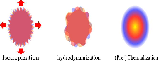
Figure 1: Schematic (conceptual) illustration of the isotropization (left), the hydrodynamization (middle), and the (pre-)thermalization (right), which respectively picturize initial quantum fluctuations with anisotropic expansion, smoothened distributions after some time, and emergence of (pre-)thermal spectra.

Figure 1 is a schematic illustration to picturize ideas of these three steps intuitively. The left picture of figure 1 is about the isotropization of the transverse pressure $P_{\rm T}$ and the longitudinal pressure $P_{\rm L}$. The ratio $P_{\rm L}/P_{\rm T}$ does not have to approach the unity, and nevertheless, it is expected to converge to a certain value instead of monotonic decrease to zero. For the realization of some time window in which $P_{\rm L}/P_{\rm T}$ can be approximately constant, it is crucial to take account of correct quantum spectrum of initial fluctuations. Although we do not go into phenomenological challenges in this review, we would note that $P_{\rm L}/P_{\rm T}$ might be (and should be) constrained by a scrupulous comparison of hydrodynamic simulations and experimental data from the heavy-ion collisions. The middle picture of figure 1 visualizes how the hydrodynamization takes place. In principle, hydrodynamic equations are conservation laws, and they are always useful as long as we are interested in slow components in real-time dynamics. For practical purposes, however, we need close a set of equations to solve them and it should be reasonable to adopt the hydrodynamic description when spacetime and momentum variations are sufficiently smoothened (and interactions are localized). It is also of pragmatic importance to resolve the hydrodynamization problem for theorizing hydrodynamics better. A recent reformulation named aHydro [6] is a clear example to extend the validity of hydrodynamics with optimal resummation. The right picture of figure 1 sketches emergence of some scaling solution that could be identified as a signature of pre-thermalization. There are several theoretical speculations such as the turbulent spectrum, the non-thermal fixed point, and the inverse Kolmogorov cascade and the resultant formation of a Bose-Einstein condensate (BEC), and so on, together with numerical demonstrations. It is, so far, not very obvious how these scenarios may or may not have an impact on heavy-ion collision phenomenology. The most serious problem lies in a technical difficulty in estimating the relevant time scale. Almost all simulations seem to require unphysically long time, hinting that something important may be still missing.

This review is organized in the following manner. After this Introduction, in section 2, we will elucidate some theoretical foundations for readers who would like to learn quickly what ideas were discussed in the past and what problems still remain today. We will start with a pedagogical introduction to the CGC theory and explain characteristic features of the CGC-type initial conditions in section 2.1. Then, as a classic example of CGC-based arguments of thermalization, in section 2.2, we will introduce what is called the “bottom-up scenario”, which underlies all thermalization ideas in contemporary approaches. We also briefly mention on the plasma and glasma instabilities afterward. In section 2.3 we discuss several theoretical methods for the real-time quantum simulation. In fact, unlike lattice discretized quantum field theories in Euclidean spacetime for which the Monte-Carlo sampling is useful, there is no general non-perturbative algorithm applicable for Minkowskian spacetime. What we can do with QCD at best is to take some limit so that a particular approximation can be validated. In the dilute limit especially when a quasi-particle approximation makes sense, the kinetic equation is the most powerful tool even for QCD and, in principle, systematic estimation of the collision term is perturbatively doable, though the numerical calculation becomes desperately heavier with higher order terms. We will flash an earliest argument of thermalization by means of the Boltzmann equation in the relaxation time approximation. In the opposite case of the dense and overpopulated limit, the semi-classical approximation would be a natural choice of most suited descriptions, which consists of the solution of the classical equations of motion and the Wigner function. In quantum mechanics the semi-classical approximation works for many problems, but for quantum field theories, the semi-classical approximation or the classical statistical simulation has delicate subtleties affected by ultraviolet (UV) modes for which the density is small and the approximation inevitably breaks down. In section 2.4 we will also give very short remarks on some unconventional approaches such as the Kadanoff-Baym equations, stochastic quantization, and gauge/gravity correspondence. Successful examples for specific problems with these techniques exist and there may be some potential for the future, but so far the applicability is limited to rather academic considerations.

We will continue to section 3, section 4, and section 5 to go into more detailed discussions on the issues of the isotropization, the hydrodynamization, and the pre-thermalization, respectively. We put our emphasis on the self-contained derivations of more or less established physics in section 2, while in later sections we will pick up and outline some of most recent results. Specifically, we will mainly focus on selected results on the classification of scaling solutions, the success of the aHydro formulation, and the speculative scenario of a gluonic BEC formation. Readers interested in hydrodynamic simulations together with a comparison to heavy-ion data can consult a recent review [7]. Because the thermalization problem is a rapidly growing subject, new progresses are steadily reported. We will not try to make this review comprehensive in vain but will take a more pragmatic strategy to explicate the problems and the progresses rather than to give an answer. For the most state-of-the-art outcomes, readers are encouraged to study further with proceedings contributions for Quark Matter conference series.

2 Theoretical Foundations

We will exposit some theoretical formulations based on QCD that are useful to quantify microscopic processes of the evolution to the QGP.  The early time dynamics in the heavy-ion collision has a universal scale called the saturation momentum (denoted as $Q_{\rm s}$) apart from the typical QCD scale, $\Lambda_{\rm QCD}$. So, it is indispensable to implement $Q_{\rm s}$ properly for modern approaches to the thermalization problem.

2.1 Small-x Physics and Color Glass Condensate

An old-fashioned quark model tells us that the nucleon is composed from three valence quarks. Such a naive picture could hold, however, for the net quantum number only and there should be a far richer structure with sea quarks and gluons once quantum corrections are included. In the infinite momentum frame in which the nucleon has an infinitely large momentum, the life time of virtual excitations is elongated due to Lorentz time dilatation, so that the parton distribution functions including virtual excitations become well-defined physical observables. A parton with a large momentum can radiate softer partons one after another in quantum processes, and there should be more abundant partons with smaller momenta. To quantify this, it is convenient to introduce Bjorken’s x that is a fraction of the longitudinal momentum carried by a parton over the total momentum of a projectile. According to the data from Hadron Electron Ring Accelerator (HERA) the gluon distribution function is about twenty times larger than the quark distribution function already around $\mathrm{x}\sim 10^{-2}$, and in the first approximation, we can neglect contributions from quarks.

For the thermalization problem, we should consider processes involving soft momenta $\lesssim 1\,\mbox{GeV}$ and then the relevant $\mathrm{x}$ is roughly $\mathrm{x}\sim 10^{-2}$ for RHIC energy of $200\,\mbox{GeV}$/nucleon and $\mathrm{x}\sim 10^{-3}$ for LHC energy of $5.5\,\mbox{TeV}$/nucleon. In this small-$\mathrm{x}$ regime, we can safely limit our considerations to gluonic contributions only using the pure Yang-Mills theory instead of full QCD with dynamical quarks. Further simplification occurs at sufficiently small $\mathrm{x}$: when the gluon distribution function $G(\mathrm{x},Q)$ where $Q$ represents the transverse momentum is such enhanced, gluons eventually saturate the transverse area $\pi R_{A}^{2}$ of the nucleon or nucleus. We should note that this happens in a way dependent on $\mathrm{x}$. Actually, the transverse size of the probed parton is characterized by $Q^{-1}$ in the Breit frame and thus the corresponding interaction cross section is $\sim\alpha_{\rm s}N_{\rm c}Q^{-2}$. Then, the saturation condition reads: $\alpha_{\rm s}N_{\rm c}G(\mathrm{x},Q_{\rm s})Q_{\rm s}(\mathrm{x})^{-2}/(N_{\rm c}^{2}-1)\simeq\pi R_{A}^{2}$. It is obvious that the left-hand side is the total cross section per one color. The solution of this equality yields a qualitative definition of the saturation scale $Q_{\rm s}(\mathrm{x})$. The most important implication from the saturation is that physical quantities should scale with $Q_{\rm s}(\mathrm{x})$ in a universal way. More concretely, as a consequence of the saturation, the total cross section $\sigma_{\gamma^{\ast}p}(\mathrm{x},Q^{2})$ of a proton and a virtual photon (with an electron vertex amputated) should no longer be a function of $\mathrm{x}$ and $Q^{2}$ independently but is a function of a scaling variable $\tau\equiv Q^{2}/Q_{\rm s}^{2}(\mathrm{x})$ only. Experimental data from HERA with various combinations of $\mathrm{x}$ and $Q^{2}$ exhibit beautiful scaling behavior called the “geometric scaling” [8] with the following parametrization;

$$Q_{\rm s}^{2}(\mathrm{x})=Q_{0}^{2}(\mathrm{x}/\mathrm{x}_{0})^{-\lambda}\;,$$ (1)

where $Q_{0}=1\,\mbox{GeV}$ is pre-fixed and $\mathrm{x}_{0}=3.04\times 10^{-4}$, $\lambda=0.288$ have been determined from the data at $\mathrm{x}<10^{-2}$. This functional form is also suggested by a solution of the BFKL equation which is a linear quantum evolution equation with changing $\mathrm{x}$. Equation (1) provides us with a more quantitative definition of $Q_{s}(\mathrm{x})$ used for phenomenological applications such as the prediction of the hadron multiplicity in a KLN model [9].

It should be noted that the saturation is a sufficient condition for the geometric scaling, but may not be a necessary condition. This means that the geometric scaling may hold outside of the saturation regime and this is indeed the case in view of the experimental data: not only $\tau\lesssim 1$ but larger $\tau\gtrsim 10^{2}$ also show the scaling behavior. This experimental finding is extremely important for reality of the CGC; for $\tau\gtrsim 1$ the parton transverse size $\sim Q^{-2}$ is certainly smaller than necessary for the saturation $\sim Q_{\rm s}^{-2}$. Therefore, the validity region of the CGC must be wider than naively expected. This “extended geometric scaling” could be a consequence from quantum evolution equations with changing $\mathrm{x}$ and $Q^{2}$ that maintain the geometric scaling even beyond the saturation regime [10]. In discussions in what follows throughout this review, we shall require that the kinematic regions involving $Q^{2}\sim Q_{\rm s}^{2}(\mathrm{x})$ dominate processes of our interested physics.

In the case of the nucleus-nucleus collision, the transverse parton density is significantly enhanced with the atomic number $A$. Because the nuclear thickness scales with $A^{1/3}$, as compared to the proton case, $Q_{\rm s}^{2}(\mathrm{x})$ should be accompanied by $A^{1/3}$ which is as a large factor as $\sim 6$ for gold and lead ions. This is a tremendously large factor; the collision energy is $\sim 27$ times increased from RHIC to LHC and so relevant $\mathrm{x}$ becomes $\sim 1/27$ times smaller. Using (1) we can easily make an estimation and conclude that $Q_{\rm s}(\mathrm{x})$ is increased by a factor $\sim 2.6$ only. Thus, the CGC regime should be activated much earlier for the heavy-ion collision than for the proton, and in view of the geometric scaling in $\sigma_{\gamma^{\ast}p}$ for $\mathrm{x}<10^{-2}$, we can be confident that the CGC be a trustful description of soft gluons with momenta $\lesssim 1\,\mbox{GeV}$ or even higher.

2.1.1 CGC effective theory

The general strategy to obtain an effective theory is to integrate unwanted degrees of freedom out. We can consider an effective theory for soft gluons by regarding $\mathrm{x}$ as a separation scale of hard and soft gluons. It has been shown that integrating hard gluons out leads to a classical color source $\rho$ for soft gluons. In such a way the probability function $W_{\mathrm{x}}[\rho]$ that characterizes how $\rho$ is distributed evolves with changing $\mathrm{x}$, and the evolution of $W_{\mathrm{x}}[\rho]$ should follow from a renormalization group equation. This is actually a contemporary derivation of the BFKL equation not from each Feynman diagram but from the invariance of the partition function [11] and its non-linear extension, i.e., the JIMWLK equation [12, 13, 14, 15] was derived as an extension of this method.

Soft gluons are thus given by a classical solution of the Yang-Mills equations of motion sourced by $\rho$ whose distribution is dictated by $W_{\mathrm{x}}[\rho]$. In a frame where the proton or the heavy-ion is moving at the speed of light in the positive $z$ direction, the color source is static in terms of the light-cone time, i.e. $\rho=\rho(x^{-},\boldsymbol{x})$ where $x^{\pm}=(t\pm z)/\sqrt{2}$ and $\boldsymbol{x}$ refers to the 2-dimensional transverse coordinates. The Yang-Mills equations to be solved then read:

$$\mathcal{D}_{\mu}\mathcal{F}^{\mu\nu}=\delta^{\nu+}\rho(x^{-},\boldsymbol{x})\;.$$ (2)

In this review we consistently use calligraphy letters to represent classical fields. We here work in the light-cone gauge with $\mathcal{A}^{+}=0$ and we assume $\mathcal{A}^{-}=0$ to solve (2). Then, let us take a static color rotation to gauge $\mathcal{A}^{i}$ away. Because of $x^{+}$ independence, such a gauge rotation $V(x^{-},\boldsymbol{x})$ does not affect $\mathcal{A}^{-}=0$ (which is confirmed from $V^{\dagger}\partial^{-}V=0$, where we should note that $\partial^{-}=\partial_{+}=\partial/\partial x^{+}$). In this rotated color basis, hence, (2) is reduced to the standard 2-dimensional Poisson equation for $\mathcal{A}^{+}$ and it is easy to find the solution as $\mathcal{A}^{+}(x^{-},\boldsymbol{x})=-\boldsymbol{\nabla}^{-2}\rho(x^{-},\boldsymbol{x})$ [4]. We can immediately rotate this solution back to the light-cone gauge using the rotation matrix $V$ and finally we arrive at the following solution:

$$\mathcal{A}^{i}=\alpha^{i}\equiv-\frac{1}{\rmi g}V(x^{-},\boldsymbol{x})\partial^{i}V^{\dagger}(x^{-},\boldsymbol{x})\;,\qquad\mathcal{A}^{\pm}=0\;,$$ (3)

where the rotation matrix to eliminate $\mathcal{A}^{+}$ is found to be

$$V^{\dagger}(x^{-},\boldsymbol{x})=\mathcal{P}\exp\biggl{[}-\rmi g\int_{-\infty}^{x^{-}}\rmd\xi^{-}\;\boldsymbol{\nabla}^{-2}\rho(\xi^{-},\boldsymbol{x})\biggr{]}\;.$$ (4)

Here, $\mathcal{P}$ stands for the time ordering. Now we are ready to compute physical observables such as the energy-momentum tensor given in terms of $\alpha^{i}$. We can write the expectation value of an arbitrary operator $\mathcal{O}[\alpha^{i}]$ (for example, $\mathcal{O}[\alpha^{i}]=\tr[V(\infty,\boldsymbol{x})V^{\dagger}(\infty,\boldsymbol{y})]$ for a dipole scattering amplitude) down as follows:

$$\langle\mathcal{O}[\alpha^{i}]\rangle=\int\rmd\rho\,W_{\mathrm{x}}[\rho]\,\mathcal{O}[\alpha^{i}]\;.$$ (5)

The above-mentioned calculational scheme with classical fields $\mathcal{A}^{\mu}$ and the weight function $W_{\mathrm{x}}[\rho]$ is commonly referred to as the color glass condensate or CGC (for a review; see [16]); in the first approximation $\rho$ is a random color source, which is reminiscent of the theory of spin glass, and is described by classical fields as if they were condensates in scalar theories prescribed by the Gross-Pitaevskii equation, which explains the name of the color glass condensate.

It should be noted that solving the classical equations of motion is an efficient resummation technique to take account of infinite Feynman diagrams at once, especially for a special case when both terms in the covariant derivative, $\mathcal{D}_{\mu}=\partial_{\mu}-ig\mathcal{A}_{\mu}$, are comparable. In the CGC regime, actually, $\partial_{\mu}$ picks up an energy and momentum scale $\sim Q_{\rm s}$. Also, the color source should be as large as $\rho\sim Q_{\rm s}/g$ and thus $\mathcal{A}_{\mu}\sim Q_{\rm s}/g$. Then, the perturbation theory must be reorganized not around the vacuum but around the CGC background fields $\mathcal{A}_{\mu}$. Such reorganized perturbative calculations result in the renormalization group flow of $W_{\mathrm{x}}[\rho]$ and the presence of $\mathcal{A}_{\mu}$ makes an upgrade of the BFKL equation into the JIMWLK equation. We should note that perturbative calculations can be useful for $\partial_{\mathrm{x}}W_{\mathrm{x}}[\rho]$ but cannot figure out $W_{\mathrm{x}}[\rho]$ itself. So, we need to rely on some empirical parametrization for $W_{\mathrm{x}}[\rho]$ at some initial $\mathrm{x}$. The simplest choice is a Gaussian Ansatz [17, 18], that is;

$$W_{\mathrm{x}}[\rho]=\exp\biggl{[}-\int\rmd^{2}\boldsymbol{x}\,\rmd x^{-}\,\frac{|\rho(x^{-},\boldsymbol{x})|^{2}}{2g^{2}\mu_{\rm x}^{2}(x^{-})}\biggr{]}\;.$$ (6)

In terms of a color component, $\rho=\rho^{a}t^{a}$ where $t^{a}$ is an element of color-group algebra in the fundamental representation, the above Gaussian form is equivalent to requiring the two-point function as $\langle\rho^{a}(x^{-},\boldsymbol{x})\rho^{b}(y^{-},\boldsymbol{y})\rangle=g^{2}\mu_{\rm x}^{2}(x^{-})\,\delta^{ab}\,\delta(x^{-}-y^{-})\,\delta^{(2)}(\boldsymbol{x}-\boldsymbol{y})$. This choice of the weight function in (6) defines what is known as the McLerran-Venugopalan (MV) model and, naturally, a unique scale $\mu_{\rm x}(x^{-})$ is related to $Q_{\rm s}(\mathrm{x})$: parametrically $Q_{\rm s}\sim g^{2}\mu_{\rm x}$ so that $\mathcal{A}_{\mu}\sim Q_{\rm s}/g$. Typically $\mu_{\rm x}$ is chosen around $1\,\mbox{GeV}$ for RHIC and $2$-$3$ times greater for LHC.  The Gaussian choice has an advantage that we can perform analytical calculations for the color average in (5), which in most cases simplifies significantly in the large $N_{\rm c}$ limit (see [19] for useful mathematical formulas).

2.1.2 Initial condition for the relativistic heavy-ion collision

The same idea of saturation physics can be applied to the relativistic heavy-ion collision and in this case both the target and the projectile are dense objects. To take full account of non-linear color fields from both nuclei, the Yang-Mills equations that we must solve read:

$$\mathcal{D}_{\mu}\mathcal{F}^{\mu\nu}=\delta^{\nu+}\rho^{(1)}(x^{-},\boldsymbol{x})+\delta^{\nu-}\rho^{(2)}(x^{+},\boldsymbol{x})\;.$$ (7)

Here (1) and (2) in the upper subscript refer to the nuclei moving in the positive and the negative $z$ directions, respectively. Unlike the single-source problem in (2), we cannot generally solve (7) in an analytically closed form. In the spacelike regions two sources cannot communicate with each other because of causality, and so the problem is to be reduced to the one-source problem. Imposing continuity from these solutions, we can at best write the analytical solution down on the light cone. For the description of the heavy-ion collision, the Bjorken coordinates $(\tau,\eta)$ are more useful than the light-cone coordinates $x^{\pm}$, which are related as

$$\sqrt{2}x^{\pm}=\tau\,\rme^{\pm\eta}\;.$$ (8)

Then, in the radial gauge $\mathcal{A}_{\tau}=x^{-}\mathcal{A}^{+}+x^{+}\mathcal{A}^{-}=0$, the solution of (7) on the light cone at $\tau=0$ takes a form of [20]

$$\mathcal{A}_{i}=\alpha^{(1)}_{i}+\alpha^{(2)}_{i}\;,\qquad\mathcal{A}_{\eta}=0\;,$$

$$\mathcal{E}^{i}=0\;,\qquad\mathcal{E}^{\eta}=\rmi g\Bigl{(}\bigl{[}\alpha_{1}^{(1)},\alpha_{1}^{(2)}\bigr{]}+\bigl{[}\alpha_{2}^{(1)},\alpha_{2}^{(2)}\bigr{]}\Bigr{)}\;,$$ (9)

where $\mathcal{E}^{i}$ and $\mathcal{E}^{\eta}$ are the transverse and the longitudinal components of the classical color electric fields. It is quite intuitive that $\mathcal{A}_{i}$ is just a linear superposition of $\alpha_{i}^{(1)}$ and $\alpha_{i}^{(2)}$, while $\mathcal{E}^{\eta}$ appears from the non-Abelian character and there is no counterpart in QED.  With this initial condition (9), we should solve the Yang-Mills Hamilton equations in the Bjorken coordinates:

$$\partial_{\tau}\mathcal{E}^{i}=\frac{1}{\tau}\mathcal{D}_{\eta}\mathcal{F}_{\eta i}+\tau\mathcal{D}_{j}\mathcal{F}_{ji}\;,\quad\partial_{\tau}\mathcal{E}^{\eta}=\frac{1}{\tau}\mathcal{D}_{j}\mathcal{F}_{j\eta}\;,$$ (10)

with the canonical conjugate momenta defined ordinarily by

$$\mathcal{E}^{i}=\tau\partial_{\tau}\mathcal{A}_{i}\;,\qquad\mathcal{E}^{\eta}=\frac{1}{\tau}\partial_{\tau}\mathcal{A}_{\eta}\;.$$ (11)

We should note that $\mathcal{E}^{\eta}$ has a correct mass dimension of the electric field but $\mathcal{E}^{i}$ does not. In physical terms $\mathcal{E}^{i}/\tau$ should be interpreted as the genuine transverse electric field which also goes to zero in the $\tau\to 0^{+}$ limit. Using $\mathcal{A}_{i}$ in (9) we can readily calculate the initial color magnetic field as

$$\mathcal{B}^{i}=0\;,\qquad\mathcal{B}^{\eta}=\mathcal{F}_{12}=-\rmi g\Bigl{(}\bigl{[}\alpha^{(1)}_{1},\alpha^{(2)}_{2}\bigr{]}+\bigl{[}\alpha^{(2)}_{1},\alpha^{(1)}_{2}\bigr{]}\Bigr{)}$$ (12)

using the fact that $\alpha_{i}^{(n)}$ is a pure gauge and so its field strength is vanishing. Although the combinations of indices for initial $\mathcal{E}^{\eta}$ in (9) and initial $\mathcal{B}^{\eta}$ in (12) are slightly different, the squared expectation values turn out to be identical after taking the color average with the Gaussian weight as defined in (6). These identical $\langle\mathcal{E}^{\eta}\mathcal{E}^{\eta}\rangle$ and $\langle\mathcal{B}^{\eta}\mathcal{B}^{\eta}\rangle$ lead us to a very suggestive profile of the initial condition for the heavy-ion collision as illustrated in figure 2.

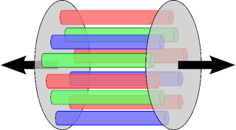
Figure 2: Schematic illustration of the glasma initial condition for the heavy-ion collision. Longitudinal color electric and magnetic fields stretch between two nucleus sheets forming a structure with color flux tubes. Figure is taken from [21].

The evolving color fields starting with the initial condition in (9) are the foundation of the “glasma” (named in [22] though its physics was known traced back to the Lund string model) which is a transient state between the color glass condensate and the quark-gluon plasma – glasma as a coined word from them. The most essential property associated with the glasma initial condition is, as sketched in figure 2, the presence of longitudinal color electric and magnetic fields with boost invariance (i.e. $\eta$ independence), which may be a source for rapidity correlation (ridge structure) [23] and also local parity violation [24]. Because $Q_{\rm s}$ is the universal scale, each color flux tube is expected to be localized in a domain whose transverse extent is $\sim Q_{\rm s}^{-1}$. In the MV model, however, it is very difficult to see such a structure by eyes. Recently the correlation length possibly related to the flux tube structure has been numerically measured in the MV model by means of spatial Wilson loops and the color flux tube picture has been partially verified [25].

For our present consideration on the thermalization problem, it is critically important to recognize that the longitudinal pressure is inevitably negative with this type of glasma initial condition. We can understand such a negative pressure intuitively: the longitudinal fields have positive energy density and so it would cost a more positive energy to stretch the color flux tubes farther. This implies that two nucleus sheets feel an attractive force to decrease the flux tube energies, leading to a negative pressure. On the algebraic level we can see this from

$$P_{\rm T}\equiv\frac{1}{2}\langle T^{xx}+T^{yy}\rangle=\Bigl{\langle}\tr\bigl{[}\mathcal{E}^{\eta a}\mathcal{E}^{\eta a}+\mathcal{F}_{12}^{a}\mathcal{F}_{12}^{a}\big{]}\Bigr{\rangle}\;,$$ (13)

$$P_{\rm L}\equiv\langle\tau^{2}T^{\eta\eta}\rangle=\frac{1}{\tau^{2}}\Bigl{\langle}\tr\bigl{[}\mathcal{E}^{ia}\mathcal{E}^{ia}+\mathcal{F}_{\eta i}^{a}\mathcal{F}_{\eta i}^{a}\bigr{]}\Bigr{\rangle}-P_{\rm T}\;.$$ (14)

In the initial stage the contribution from transverse fields is negligibly small (regardless of $1/\tau^{2}$), and so $P_{\rm T}>0$ and $P_{\rm L}\sim-P_{\rm T}<0$ should be simultaneously developing for finite but small $\tau$.

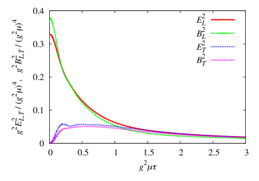
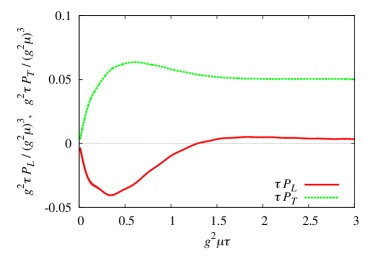
Figure 3: Typical evolution of the color electric and magnetic fields in the MV model (left) and the transverse and the longitudinal pressure (right). Figures are taken from [26].

We can numerically solve the equations of motion in (10) and (11) on lattice discretized spacetime. It is not mandatory to use the link variables for classical theories, but the conventional lattice formulation in terms of the link variables $U_{\mu}$ is convenient to stabilize long time simulations. It is then a bit cumbersome to rewrite the initial condition (9) in terms of $U_{\mu}$, which was done in [27].

Ideally the results have no dependence on the choice of $\mu_{\rm x}$ once all variables are made dimensionless in the unit of $\mu_{\rm x}$. In the actual calculation, however, this is not the case since the color average in (5) is ultraviolet (UV) and infrared (IR) singular and so the results depend on the lattice spacing $a$ and the system volume $L^{3}$. Nevertheless, such unphysical UV and IR sensitivity becomes harmlessly mild once $\tau$ gets larger than $1/a$ [3, 28, 29] (and this is why a naive expansion in terms of $\tau$ as attempted in [30] completely fails due to singular $\tau/a$ terms; see [31] for more details). Figure 3 shows a typical example of the temporal profile of the color electric and magnetic fields (left figure) and also the transverse and the longitudinal pressure (right figure) from the MV model simulation. All physical quantities are made dimensionless in the unit of $g^{2}\mu_{\rm x}\sim Q_{\rm s}$. From these figures we see that the longitudinal pressure $P_{\rm L}$ goes negatively at first and approaches zero back for $g^{2}\mu_{\rm x}\tau\gtrsim 1$. The longitudinal expansion with $P_{\rm L}=0$ means free-streaming, which will be closely discussed later in section 3. To summarize the essential features of the glasma initial condition, the color fields are boost invariant ($\eta$ independent) and the longitudinal pressure is negative. We need to find some mechanism of violating the boost invariance to decohere fields and to make $P_{\rm L}$ turn back to positive. For this purpose it is indispensable to consider quantum fluctuations properly beyond the classical approximation.

2.2 CGC-based Scenarios for Thermalization

The early-time dynamics in the heavy-ion collisions has a unique scale $Q_{\rm s}$, so that the proper unit to measure the time is $Q_{\rm s}^{-1}\sim 0.2\,\mbox{fm}/c$ for RHIC and $\sim 0.1\,\mbox{fm}/c$ for LHC.  An interesting and challenging question is whether we can somehow give an analytical estimate for the thermalization time in terms of $\alpha_{\rm s}=g^{2}/(4\pi)$ and $Q_{\rm s}$ for sufficiently small coupling $\alpha_{\rm s}\ll 1$. This program was first addressed in [32] (see also [3] for a rather negative conclusion) and the so-called “bottom-up scenario” has grown popular. Since this picture of the bottom-up thermalization contains important view points for subsequent developments (as partly seen in discussions in section 5), let us start this subsection with a review of the bottom-up thermalization.

2.2.1 Bottom-up thermalization scenario

The conclusion from the bottom-up thermalization scenario [32] is that the parametrical expressions of the thermalization time scale and the maximal temperature are, respectively,

$$Q_{\rm s}\tau_{\rm th}\sim\alpha_{\rm s}^{-13/5}\;,\qquad T/Q_{\rm s}\sim\alpha_{\rm s}^{2/5}\;.$$ (15)

To understand these results, we should first make it clear how to define thermalization.

In this scenario hard gluons with momenta $\sim Q_{\rm s}$ are initially produced and the thermalization time of soft gluons with momenta $\sim T$ is defined when the energy of hard gluons is transferred to soft gluons. Let us first consider a branching process from a hard gluon into gluons with a softer momentum $k_{\rm br}$. If there are $N_{\rm soft}$ soft gluons and their population is a thermalized one by $N_{\rm soft}\sim T^{3}$, as we explain soon later, the following relations can be shown:

$$k_{\rm br}\sim\alpha_{s}^{4}T^{3}\tau_{\rm th}^{2}\;,\qquad T\sim\alpha_{\rm s}^{3}Q_{\rm s}^{2}\tau\;.$$ (16)

Then, once these are accepted, the energy flow from hard to soft gluons should be terminated when $k_{\rm br}\sim Q_{\rm s}$, which, together with $T\sim\alpha_{\rm s}^{3}Q_{\rm s}^{2}\tau_{\rm th}$, means that $k_{\rm br}\sim\alpha_{\rm s}^{13}Q_{\rm s}^{6}\tau_{\rm th}^{5}\sim Q_{\rm s}$ leading immediately to the thermalization time scale and the initial temperature at $\tau=\tau_{\rm th}$ as given in (15).

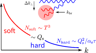
Figure 4: Schematic illustration of the bottom-up thermalization scenario.

To understand the first relation in (16) let us consider a formation time $\tau_{\rm f}$ needed for one emission process, which is estimated by the uncertainty principle as

$$\tau_{\rm f}\sim\frac{1}{k^{+}}\sim\frac{k_{\rm br}}{\Delta k_{\perp}^{2}}\;.$$ (17)

Then, the energy is deposited to the thermal medium by further hard splitting processes and the time taken by these processes defines the thermalization time $\tau_{\rm th}$. Parametrically, $\tau_{\rm f}=\alpha_{\rm s}\tau_{\rm th}\ll\tau_{\rm th}$. Now, we need to know what $\Delta k_{\perp}$ is, which reflects the thermal properties in the soft sector. Using a diffusion constant $\hat{q}\equiv\rmd\langle k_{\perp}^{2}\rangle/\rmd t$, it is obvious that $\Delta k_{\perp}^{2}\sim\hat{q}\cdot\tau_{\rm f}$, and $\hat{q}$ can be parametrized as $\hat{q}\sim m_{\rm D}^{2}/\lambda$ with the Debye mass $m_{\rm D}$ and the mean-free path $\lambda$. In a thermal medium $m_{\rm D}^{2}\sim\alpha_{\rm s}T^{2}$ and $\lambda\sim 1/(\alpha_{\rm s}T)$, which eventually yields $\hat{q}\sim\alpha_{\rm s}^{2}T^{3}$. Therefore, we can have a relation:

$$\Delta k_{\perp}^{2}\sim\frac{k_{\rm br}}{\tau_{\rm f}}\sim\alpha_{\rm s}^{2}T^{3}\tau_{\rm f}\;.$$ (18)

The first expression in (16) is a result from plugging $\tau_{\rm f}=\alpha_{\rm s}\tau_{\rm th}$ into the above.

The second in (16) originates from the energy balance. In terms of the rate of the gluon production, $\rmd N/\rmd\tau$, the energy flow per unit time should be $k_{\rm br}\cdot\rmd N/\rmd\tau$ that is equated to an increase in thermal energy by $\rmd(T^{4})/\rmd\tau$. Because softer gluons are emitted from a hard gluon whose density is $\sim Q_{\rm s}^{3}/(\alpha_{\rm s}Q_{\rm s}\tau)$ (where the gluon distribution function in the saturation regime is $\sim 1/\alpha_{\rm s}$ and $Q_{\rm s}\tau$ in the denominator represents the longitudinal expansion effect), the rate should be characterized as $\rmd N/\rmd\tau\sim Q_{s}^{2}/(\alpha_{s}\tau^{2})$. Therefore, $\rmd(T^{4})/\rmd\tau\sim T^{3}\rmd T/\rmd\tau\sim(\alpha_{s}^{4}T^{3}\tau^{2})\cdot Q_{s}^{2}/(\alpha_{s}\tau^{2})$, which concludes that the temperature grows up linearly as expressed in the second relation in (16). As discussed in the original work [32] the above-mentioned qualitative derivations can be more quantified by means of the Boltzmann equation. The Boltzmann equation is actually a very useful tool and is widely used for other scenarios like a CGC-driven BEC, as introduced in details in section 5.

2.2.2 Plasma and glasma instabilities

The prefactor of $\tau_{\rm th}$ from the bottom-up thermalization scenario is expected to be not much different from the unity. If we take the parametric estimate literally, $\alpha_{\rm s}^{-13/5}\sim 23$ for $\alpha_{\rm s}\sim 0.3$ and it is difficult to account for thermalization within a reasonable time scale, namely, a few times $Q_{\rm s}^{-1}$ or even earlier. There must be some missing mechanism that should accelerate thermalization.

It has been pointed out that a plasma in general has various instabilities and so the isotropization can be quickly driven by QCD counterparts of them, namely, QCD plasma instabilities [33]; especially, an instability induced by strong anisotropy in the momentum distribution is important [34] (see [35] for comprehensive and analytical arguments on QCD plasma instabilities). Among several instabilities, it is believed that the Weibel instability is the most relevant for the heavy-ion collisions that spontaneously forms a filamentation pattern. It would be instructive to take a look at the Weibel instability in a QED plasma with the electric current and the magnetic field $B$. Figure 5 captures the essential idea of the Weibel instability. Suppose that there is spatial inhomogeneity in $B$, electron motions are affected by the magnetic field. The upper situation in the figure shows the electron motion in one direction, and the lower in the opposite direction. In both cases the same pattern of the electric current appears as depicted in the right of the figure. Induced magnetic fields are sourced by these electric currents and new $B$ turns out to strengthen the initial spatial inhomogeneity in $B$. Since the initial disturbance is amplified each time the backreaction from electron motions is taken into account, the filamentation pattern grows up exponentially fast that signals for an instability.

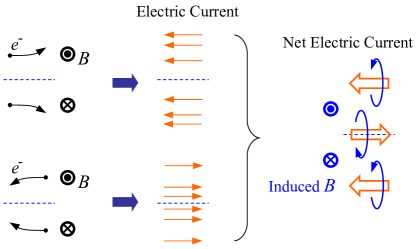
Figure 5: Schematic illustration of the Weibel instability. Spatial inhomogeneity of the magnetic field is strengthened by the backreaction of electron motions under the magnetic field.

In the pure Yang-Mills theory the system has no direct counterpart of electrons, i.e., (approximately) no quarks in the initial dynamics, and yet, gluons are color charged particles. Therefore, color magnetic fields at soft scale and color charged gluons at hard scale are sufficient ingredient for the realization of the non-Abelian Weibel instability. Let us recall that the CGC initial condition is boost invariant, and $P_{\rm L}$ is negative as long as boost-invariant color flux tubes are extending between two nuclei. Thus, it is indispensable to violate boost invariance by breaching color flux tubes with quantum fluctuations. Actually, this should be physically interpreted as particle production due to string breaking processes. Because we are interested in the fate of boost-invariant background fields $\mathcal{A}^{\mu}$, it would be convenient to introduce a Fourier transform as

$$\delta\mathcal{A}^{\mu}(\tau,\nu,\boldsymbol{k}_{\perp})\equiv\int\rmd\eta\,\rme^{-\rmi\nu\eta}\mathcal{A}^{\mu}(\tau,\eta,\boldsymbol{k}_{\perp})\;.$$ (19)

The physical meaning of $\nu$ is a dimensionless wave-number to quantify inhomogeneity along the longitudinal beam axis. Fields at $\nu=0$ represent boost-invariant backgrounds, and the definition gives a relation; $\nu=tk_{z}+zk_{0}$ (in this review, we do not distinguish covariant and contravariant vectors; $k_{z}=k^{z}$ simply, except for the notations for the light-cone and the Bjorken coordinates). Then, using this Fourier transformed variables, we can write the classical gluon fields as $2\pi\delta(\nu)\mathcal{A}^{\mu}(\tau,\boldsymbol{k}_{\perp})+\delta\mathcal{A}^{\mu}(\tau,\nu,\boldsymbol{k}_{\perp})$ with boost-invariant CGC fields and instability-driven fluctuations. As long as the latter is smaller than the former, we can investigate the instability using linearized equations of motion; i.e., in the Bjorken coordinates, the transverse fields should satisfy:

$$\partial_{\tau}\tau\partial_{\tau}\delta\mathcal{A}_{i}=-\frac{\nu^{2}}{\tau}\delta\mathcal{A}_{i}+\tau\mathcal{G}^{-1}_{ij}[\mathcal{A}]\delta\mathcal{A}_{j}\;.$$ (20)

with the full gluon propagator $\mathcal{G}^{\mu\nu}[\mathcal{A}]$ in the presence of background $\mathcal{A}^{\mu}$. If $\mathcal{G}^{-1}_{ij}$ has a positive eigenvalue $\lambda$, then the solution of the above equation should generally take the following form [29]:

$$\delta\mathcal{A}_{i}\sim c_{1}\Re I_{\rmi\nu}(\sqrt{\lambda}\tau)+c_{2}\Im I_{\rmi\nu}(\sqrt{\lambda}\tau)\;,$$ (21)

where $I_{\rmi\nu}(\sqrt{\lambda}\tau)$ is the modified Bessel function. Given some initial condition, the evolution of $\delta\mathcal{A}^{\mu}(\tau)$ is deterministic, and its time dependence should be exponential if $c_{1}\neq 0$ in the above.

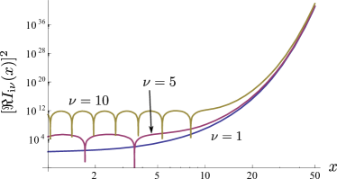
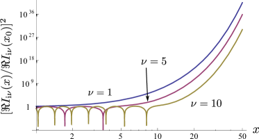
Figure 6: Typical behavior of unstable modes in one-dimensionally expanding systems. (Left) Squared quantities of the modified Bessel functions for $\nu=1$, $5$, and $10$. (Right) Squared quantities of the modified Bessel functions normalized at $x_{0}=0.1$.

Let us take an even closer look at $\Re I_{\rmi\nu}(x)$ to have an intuitive feeling about instabilities in one-dimensional expanding systems. Figure 6 plots $[\Re I_{\rmi\nu}(x)]^{2}$ in two different ways. The left figure shows the values of the functions as they are for $\nu=1$, $5$, and $10$. We see that the oscillatory behavior lasts longer for larger $\nu$, which can be easily explained from (10). As long as the first term enhanced by $\nu^{2}/\tau$ overwhelms the right-hand side, no unstable behavior appears. This observation fits in with our intuition: the expansion tends to inhibit instability. The oscillatory region itself, however, does not delay the onset of instability as is the case in the left of figure 6, showing asymptotic convergence to the same curve. In most physical cases the weight for larger-$\nu$ modes should be more suppressed (otherwise, $\Re I_{\rmi\nu}(x)$ becomes unphysically large as $\nu$ increases), and to see this effect, the right of figure 6 shows $[\Re I_{\rmi\nu}(x)/\Re I_{\rmi\nu}(x_{0}=0.1)]^{2}$, so that different $\nu$ modes are all normalized at $x=x_{0}$. Then, for larger $\nu$, the weight is smaller and the waiting time for instability becomes larger [29, 36]. Because such delaying effects are so sensitive to $\nu$-dependent weight, we must know the spectrum of initial fluctuations very precisely to locate the onset of instabilities and to account for early isotropization quantitatively.

Now let us return to discussions on the QCD Weibel instability. There are many analytical and numerical studies on the Weibel instability and it is not realistic to try to cover all of them here. As a typical and comprehensible example, let us pick up one fairly analytical formulation in [37] (see also related numerical works [38, 39]). The basic setup is a combination of the Yang-Mills equation and the Vlasov equation (or Wong’s equation in [38]). The color fields represent the soft components of gluons as is naturally implemented in the CGC theory. The hard components are split into the color-neutral part and the colored part. The neutral part is assumed to have anisotropic distribution,

$$f_{0}(\boldsymbol{k})=f_{\rm iso}(\sqrt{\boldsymbol{k}_{\perp}^{2}+k_{\eta}^{2}/\tau_{\rm iso}^{2}})\;,$$ (22)

where $f_{\rm iso}(\boldsymbol{k})$ is an isotropic distribution function. The colored part, $\delta f^{a}(\boldsymbol{k},x)$, that represents a counterpart of electrons in figure 5, should be then determined by the Vlasov equation that reads (with the collision term neglected):

$$k_{\alpha}\mathcal{D}^{\alpha ab}\delta f^{b}(\boldsymbol{k}_{\perp},k_{\eta})=gk_{\alpha}\mathcal{F}^{\alpha\beta a}\frac{\partial}{\partial p^{\beta}}f_{0}(\boldsymbol{k}_{\perp},k_{\eta})\;,$$ (23)

in the Bjorken coordinates. Once $\delta f^{a}(\boldsymbol{k}_{\perp},k_{\eta})$ is solved, the color fields should satisfy the Yang-Mills equations with a color source provided by $\delta f^{a}(\boldsymbol{k}_{\perp},k_{\eta})$, that is,

$$\frac{1}{\tau}\mathcal{D}_{\alpha}^{ab}(\tau\mathcal{F}^{\alpha\beta b})=j^{\beta a}=\frac{g}{2}\int\frac{\rmd^{2}\boldsymbol{k}_{\perp}\,\rmd y}{(2\pi)^{3}}\,k^{\beta}\,\delta f^{a}(\boldsymbol{k}_{\perp},k_{\eta})\;,$$ (24)

where $y\equiv\mathrm{atanh}(k_{0}/k_{z})$. The information on the isotropic distribution is totally encompassed in the Debye mass, which is defined in terms of the distribution function as

$$m_{\rm D}^{2}\equiv g^{2}\int_{0}^{\infty}\frac{\rmd^{3}\boldsymbol{k}}{(2\pi)^{3}2\omega(\boldsymbol{k})}\,f_{\rm iso}(\boldsymbol{k})\;.$$ (25)

It must be noted that $f_{\rm iso}(\boldsymbol{k})$ in the above is spin-summed and color-averaged one; if the distribution function is the one per spin and color, the definition of $m_{\rm D}^{2}$ should be multiplied by $2C_{A}=2N_{\rm c}$, which more often appears in the literature. The linearized Yang-Mills equations after eliminating $\delta f^{a}(\boldsymbol{k}_{\perp},k_{\eta})$ should dictate the temporal evolution of fluctuation modes and, for late time $\tau\gg\tau_{0}\gg\tau_{\rm iso}$ where $\tau_{0}$ represents the initial time, the Yang-Mills equations are reduced to

$$\bigl{[}\partial_{\tau}^{2}\tau\partial_{\tau}\tau\partial_{\tau}+\nu^{2}\partial_{\tau}^{2}+\mu\partial_{\tau}^{2}\tau-\mu\nu^{2}\tau^{-1}\bigr{]}\delta\mathcal{A}^{i}(\tau,\nu)=0\;,$$ (26)

$$\bigl{[}\partial_{\tau}\tau^{-1}\partial_{\tau}+2\mu\tau^{-2}\bigr{]}\delta\mathcal{A}_{\eta}(\tau,\nu)=0\;,$$ (27)

where $\mu\equiv\frac{\pi}{8}m_{\rm D}^{2}\tau_{\rm iso}$, which actually represent the concrete contents of (10). These are easily solvable using the (modified) Bessel functions. In fact, $\delta\mathcal{A}_{\eta}(\tau,\nu)$ can be given by a linear superposition of oscillatory Bessel functions and thus it is concluded that $\delta\mathcal{A}_{\eta}(\tau,\nu)$ has no instability in the linear regime. It is found that, even for $\nu\gg 1$ (which is less unstable according to the previous discussions) $\delta\mathcal{A}^{i}(\tau,\nu)$ is a linear superposition of modified Bessel functions as

$$\delta\mathcal{A}^{i}(\tau,\nu\gg 1)\simeq c_{1}\,\sqrt{\tau}I_{1}(2\sqrt{\mu\tau})+c_{2}\,\sqrt{\tau}K_{1}(2\sqrt{\mu\tau})\;,$$ (28)

which is an exponentially growing function and this diverging behavior manifests the non-Abelian Weibel instability. The appearance of $\sim I_{n}(c\sqrt{\mu\tau})\sim(\mu\tau)^{-1/4}\rme^{c\sqrt{\mu\tau}}$ is typical in one-dimensional expanding systems; the exponential growth is not like $\sim\rme^{c\tau}$ but $\sim\rme^{c\sqrt{\mu\tau}}$ due to expansion.

In the approach with the Vlasov and the Yang-Mills equations the separation between the field of soft gluons and the particle of hard gluons seems to be an artificial choice. In principle, the physical results should not depend on where the separation scale is, but it is quite non-trivial to verify this (see [39] for an example of explicit check). It would be desirable to build a simple and unifying description to deal with both soft and hard components within a common framework. Promising results actually came out from the glasma simulation with initial fluctuations incorporated.

Instead of solving coupled equations for $\mathcal{A}_{\mu}$ and $\delta f^{a}(\boldsymbol{k})$ and integrating $\delta f^{a}(\boldsymbol{k})$ out, we can directly write down a counterpart of (10) by linearizing the classical Yang-Mills equations with $2\pi\delta(\nu)\mathcal{A}^{\mu}(\tau,\boldsymbol{k}_{\perp})+\delta\mathcal{A}^{\mu}(\tau,\nu,\boldsymbol{k}_{\perp})$. In fact, we do not have to perform the linearization, but we can just solve the full classical Yang-Mills equations with initial fluctuation seeds $\delta\mathcal{A}^{\mu}(\tau,\nu,\boldsymbol{k}_{\perp})$ to break boost invariance. In this way, unstable behavior has been discovered, which is referred to as glasma instability [40]. Physically speaking, by construction, the origin of the glasma instability should be the same as that of the plasma (Weibel) instability as emphasized in [41], but there is no clear correspondence between the glasma and the plasma instabilities on the algebraic level. In a sense, as numerically observed in figure 7 for example, the glasma instability could be understood as a diffusion process in $\nu$ space from the CGC field at $\nu=0$ to higher $\nu$ modes, which was investigated by mode-by-mode analysis in [26], and a sort of avalanche behavior was verified in [42] (see also [39] in which the UV avalanche was first pointed out). This is an example of the self-similarity and the spectral cascade phenomenon that will be more discussed in section 3 and section 5. We also note that the classical Yang-Mills equations are highly non-linear, and so there may be instabilities associated with chaotic behavior of solutions [43]. In fact, in some numerical simulations [44, 45], the Lyapunov exponents have been extracted, which is useful for the computation of the Kolmogorov-Sinai entropy [46].

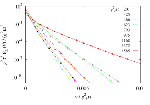
Figure 7: Spectral decomposition of the CGC electric energy density as a function of wave-number $\nu$ for various time $\tau$. Initially all the energy is stored only at $\nu=0$, which diffuses to larger $\nu$ as the time goes. Figure is taken from [26].

2.3 Real-time Formulations

We have already previewed some results from the kinetic equation and the classical field. The former is effective for a regime where the gluon distribution is dilute. Once the gluon amplitude reaches the saturation regime, the expansion of the collision term with respect to the gluon distribution does not work, and the classical approximation makes better sense. The semi-classical method has been highly sophisticated into a form of the classical statistical approximation nowadays, which, however, may suffer the UV singularities. Finally, we will quickly look over some other methods.

2.3.1 Dilute regime — kinetic equation

Let us begin with a classical example of simple scalar field theory. In the dilute regime at weak coupling, the Boltzmann equation should be an appropriate description of the real-time dynamics. For the distribution function $f(\boldsymbol{k},\boldsymbol{x},t)$ the scalar Boltzmann equation reads:

$$\frac{\rmd f}{\rmd t}=\biggl{(}\frac{\partial}{\partial t}+\dot{\boldsymbol{x}}\frac{\partial}{\partial\boldsymbol{x}}+\dot{\boldsymbol{k}}\frac{\partial}{\partial\boldsymbol{k}}\biggr{)}f(\boldsymbol{k},\boldsymbol{x},t)=\biggl{(}\frac{\partial f}{\partial t}\biggr{)}_{\rm coll}\;,$$ (29)

where the last term represents the collision term, which can be diagrammatically calculated at weak coupling. The simplest example is an elastic $2\leftrightarrow 2$ process, for which the collision term should take a conventional expression,

$$\biggl{(}\frac{\partial f(\boldsymbol{k}_{1})}{\partial t}\biggr{)}_{2\leftrightarrow 2} = \frac{1}{4\nu\,\omega(\boldsymbol{k}_{1})}\int_{\boldsymbol{k}_{2},\boldsymbol{k}_{3},\boldsymbol{k}_{4}}(2\pi)^{4}\delta^{(4)}(k_{1}+k_{2}-k_{3}-k_{4})\,|\mathcal{M}_{2\leftrightarrow 2}(\boldsymbol{k})|^{2}$$ (30)

$$\quad\times\Bigl{\{}f_{3}f_{4}(1+f_{1})(1+f_{2})-f_{1}f_{2}(1+f_{3})(1+f_{4})\Bigr{\}}\;.$$

Here we introduced a compact notation; $\int_{\boldsymbol{k}}\equiv\int\,\rmd^{3}\boldsymbol{k}/[2\omega(\boldsymbol{k})(2\pi)^{3}]$ with $\omega(\boldsymbol{k})=|\boldsymbol{k}|$ for massless bosons, $f_{i}\equiv f(\boldsymbol{k}_{i})$, and $\nu$ represents the degeneracy factor associated with internal quantum number (such as spin degeneracy). When the system gets equilibrated, $\rmd f/\rmd t=0$ and so the detailed balance is realized, from which the Bose-Einstein distribution function is derived as follows. Let us require that $f_{3}f_{4}(1+f_{1})(1+f_{2})-f_{1}f_{2}(1+f_{3})(1+f_{4})=0$ for arbitrary $\boldsymbol{k}_{1}$, $\boldsymbol{k}_{2}$, $\boldsymbol{k}_{3}$, and $\boldsymbol{k}_{4}$, which is a sufficient (but not necessary) condition to let the collision term vanish. Then, by taking logarithms, we can show,

$$\ln\biggl{(}\frac{1+f_{1}}{f_{1}}\biggr{)}+\ln\biggl{(}\frac{1+f_{2}}{f_{2}}\biggr{)}=\ln\biggl{(}\frac{1+f_{3}}{f_{3}}\biggr{)}+\ln\biggl{(}\frac{1+f_{4}}{f_{4}}\biggr{)}\;.$$ (31)

This means that $\ln[(1+f)/f]$ should be a conserved quantity, and so should be expressed as a linear combination of basic conserved quantities; $1$, $\boldsymbol{k}$, and $k^{0}=\omega(\boldsymbol{k})$ as

$$\ln\biggl{[}\frac{1+f(\boldsymbol{k})}{f(\boldsymbol{k})}\biggr{]}=\frac{\mu}{T}-\frac{k^{\mu}u_{\mu}}{T}\quad\Rightarrow\quad f(\boldsymbol{k})=\frac{1}{\rme^{(k^{\mu}u_{\mu}-\mu)/T}-1}\;.$$ (32)

Here, $u_{\mu}$ represents the fluid four-velocity.

The thermalization problem of the QGP or the isotropization in modern language was first investigated in [2] using the Boltzmann equation with the relaxation time approximation (RTA). Because the calculations are quite instructive to explain the basic features of the QGP, below, we shall reiterate the main steps of calculations in [2]. In the heavy-ion collision the system cannot be homogeneous in the Cartesian coordinates because the longitudinal velocity is $u=z/t$ and the Lorentz time dilatation becomes greater for larger $z$. So, we should keep $\partial/\partial z$ in the left-hand side of (29), while $\dot{\boldsymbol{k}}$ drops off without external force. Then, once boost invariance is imposed, $z$ dependence is uniquely fixed through $k_{z}(z)=\gamma(k_{z}-k_{0}u)$ where $k_{z}$ and $k_{0}$ are the longitudinal momentum and the energy at $z=0$. From this, it is easy to see that $\partial/\partial z=-(k_{0}/t)\partial/\partial k_{z}$ if they act on a function of $k_{z}(z)$. Therefore, in this case of boost-invariant expansion, the Boltzmann equation takes a form of

$$\biggl{(}\frac{\partial}{\partial t}-\frac{k_{z}}{t}\frac{\partial}{\partial k_{z}}\biggr{)}f(\boldsymbol{k}_{\perp},k_{z},t)=\biggl{(}\frac{\partial f}{\partial t}\biggr{)}_{\rm coll}\;,$$ (33)

apart from transverse dynamics that we neglect. Below we drop $z$ from $f(\boldsymbol{k}_{\perp},k_{z},z,t)$ focusing on the mid rapidity region only. In the absence of collision, we have the free-streaming solution; i.e., $f(\boldsymbol{k}_{\perp},k_{z},t)=f(\boldsymbol{k}_{\perp},k_{z}t/t_{0})$ solves (33). In the free-streaming case, the local energy density becomes,

$$\qquad\qquad\varepsilon(t)=\int\frac{\rmd^{3}\boldsymbol{k}}{(2\pi)^{3}}|\boldsymbol{k}|\,f(\boldsymbol{k},t)=\frac{t_{0}}{t}\int\frac{\rmd^{2}\boldsymbol{k}_{\perp}\rmd\xi}{(2\pi)^{3}}\sqrt{\boldsymbol{k}_{\perp}^{2}+\xi^{2}}\,f_{0}(\boldsymbol{k}_{\perp},\xi)\;\propto\;\frac{1}{t}\;,$$ (34)

which is a natural consequence from one-dimensional expansion. In the RTA in which the analytical calculation is feasible, the collision term is assume to be as simple as

$$\biggl{(}\frac{\partial f}{\partial t}\biggr{)}_{\rm coll}=-\frac{1}{\tau_{\rm rel}}\bigl{[}f(\boldsymbol{k}_{\perp},k_{z},t)-f_{\rm eq}(\boldsymbol{k},t)\bigr{]}\;,$$ (35)

where $\tau_{\rm rel}$ represents the relaxation time and $f_{\rm eq}(\boldsymbol{k},t)$ is the Bose-Einstein distribution function at the temperature $T(t)$. Generally speaking, $\tau_{\rm rel}$ is a function of time and momenta, but if we adopt a constant $\tau_{\rm rel}$, we can analytically solve the Boltzmann equation under the initial condition of $f(\boldsymbol{k}_{\perp},k_{z},t=t_{0})=f_{0}(\boldsymbol{k}_{\perp},k_{z})$ as

$$f(\boldsymbol{k}_{\perp},k_{z},t)=\rme^{(t_{0}-t)/\tau_{\rm rel}}f_{0}(\boldsymbol{k}_{\perp},k_{z}t/t_{0})+\int_{t_{0}}^{t}\frac{\rmd t^{\prime}}{\tau_{\rm rel}}\,\rme^{(t^{\prime}-t)/\tau_{\rm rel}}\,f_{\rm eq}(\sqrt{\boldsymbol{k}_{\perp}^{2}+(k_{z}t/t^{\prime})^{2}},t^{\prime})\;.$$ (36)

From this form of the solution, an integral equation for $\varepsilon(t)$ can be derived [2], which can be solved for $t\gg\tau_{\rm rel}$ (with the energy conservation and an assumption that the initial distribution is peaked at $p^{z}=0$) leading finally to

$$\frac{\varepsilon(t)}{\varepsilon(t_{0})}\simeq 1.22\;\frac{t_{0}\tau_{\rm rel}^{1/3}}{t^{4/3}}\;\propto\;\frac{1}{t^{4/3}}\;.$$ (37)

This $t$ dependence makes a sharp contrast to the free-streaming one in (34) and should be interpreted as the complete isotropization. Actually, the conservation equation in the expanding system reads:

$$\frac{\rmd\varepsilon}{\rmd\tau}+\frac{\varepsilon+P_{\rm L}}{\tau}=0\;,$$ (38)

where $P_{\rm L}$ is the longitudinal pressure as defined in (14). If $P_{\rm L}=0$ in the free-streaming case, $\varepsilon\sim 1/\tau$ as we have already seen in (34). (It should be noted that we took $z=0$ to simplify discussions, so that $\tau$ is just $t$ then.) Once $P_{\rm L}=P_{\rm T}$ is realized and the conformality is approximately realized as $\varepsilon-2P_{\rm T}-P_{\rm L}\approx 0$, then $P_{\rm L}\approx\varepsilon/3$ and we see that $\varepsilon\sim 1/\tau^{4/3}$ is concluded from (38). In summary, if the interaction is turned off, the free-streaming solution leads to $\varepsilon\propto 1/\tau$, and if the interaction is strong enough to achieve the complete isotropization, the hydrodynamic scaling (in a sense of old-fashioned characterization) follows as $\varepsilon\propto 1/\tau^{4/3}$. In reality it is quite unlikely that the system can be fully isotropized in the heavy-ion collisions and the exponent should be something between $-1$ and $-4/3$. For the reliable determination of the exponent, the RTA is a too crude approximation, and the most serious obstacle is that the RTA would violate conservation laws, which may be cured in the Lorentz model, but it should be of course much better if the QCD interaction is systematically considered.

Figure 8: The collisions terms of $2\leftrightarrow 2$ scattering (upper) and $1\leftrightarrow 2$ scattering (lower). The reversed processes to increase $1$ are omitted.

For this purpose the effective kinetic theory (EKT) of QCD [47] has been developed, with which the shear viscosity calculation is performed and also the jet energy loss is evaluated. The EKT consists of the Boltzmann equation with two scattering terms; an elastic $2\leftrightarrow 2$ scattering and an inelastic $1\leftrightarrow 2$ scattering. The former is easy to find from the usual Feynman rule. Because the triple-gluon vertex has one derivative, for example, the $t$-channel scattering in the upper left in figure 8 leads to $|(k_{1}+k_{3})\cdot(k_{2}+k_{4})/(k_{3}-k_{1})^{2}|=(s-u)^{2}/t^{2}=1-4us/t^{2}$ using the Mandelstam variables, $s=(k_{1}+k_{2})^{2}$, $t=(k_{1}-k_{3})^{2}$, and $u=(k_{1}-k_{4})^{2}$ with four-vector notation. Summing the $u$-channel and $s$-channel contributions up together with the quartic-gluon vertex term, the $2\leftrightarrow 2$ matrix element eventually amounts to

$$|\mathcal{M}_{2\leftrightarrow 2}|^{2}=16g^{4}d_{A}C_{A}^{2}\biggl{(}3-\frac{us}{t^{2}}-\frac{st}{u^{2}}-\frac{tu}{s^{2}}\biggr{)}\;,$$ (39)

where $d_{A}=N_{\rm c}^{2}-1$ and $C_{A}=N_{\rm c}$.

In contrast to this, the $1\leftrightarrow 2$ scattering is much more complicated because in this case, if all gluons are massless, only the completely collinear scattering is kinematically possible, and the quantum destructive interference effect with multiple scatterings with surrounding media called the Landau-Pomeranchuk-Migdal (LPM) effect should be taken into account. So, apart from small finite angles allowed by the effective gluon mass, we can postulate $\boldsymbol{k}_{2}=k_{2}\hat{\boldsymbol{k}}_{1}$ and $\boldsymbol{k}_{3}=k_{3}\hat{\boldsymbol{k}}_{1}$ (where $k_{i}$ represents not four-vector but $k_{i}=|\boldsymbol{k}_{i}|$ in expressions below) in the lower processes in figure 8. The collision term for the $1\leftrightarrow 2$ scattering involves two different kinds of contributions corresponding to two diagrams in figure 8. Now, since the vector directions of $\boldsymbol{k}_{2}$ and $\boldsymbol{k}_{3}$ are fixed, we can readily take the angle integrations to express the collision term as

$$\biggl{(}\frac{\partial f(\boldsymbol{k}_{1})}{\partial t}\biggr{)}_{1\leftrightarrow 2}=\frac{(2\pi)^{3}}{2|\boldsymbol{k}_{1}|^{2}\nu}\int_{0}^{\infty}\rmd k_{2}\rmd k_{3}$$

$$\qquad\times\Bigl{[}\delta(k_{1}-k_{2}-k_{3})\gamma(\boldsymbol{k}_{1};\boldsymbol{k}_{2},\boldsymbol{k}_{3})\Bigl{\{}f_{2}f_{3}(1+f_{1})-f_{1}(1+f_{2})(1+f_{3})\Bigr{\}}$$

$$\qquad\quad+2\delta(k_{1}+k_{2}-k_{3})\gamma(\boldsymbol{k}_{3};\boldsymbol{k}_{1},\boldsymbol{k}_{2})\Bigl{\{}f_{3}(1+f_{1})(1+f_{2})-f_{1}f_{2}(1+f_{3})\Bigr{\}}\Bigr{]}\;.$$ (40)

The scattering rate $\gamma(\boldsymbol{k}_{i};\boldsymbol{k}_{j},\boldsymbol{k}_{k})$ should contain multiple interactions with media and should reproduce the leading-order LPM effect. The explicit form is given in [47] in a form of the integral equation.

It is not easy to solve these functional equations numerically, and the state-of-the-art numerical simulation with these equations has been carried out in [48]. The central message from [48] is summarized in a schematic picture in figure 9, which is adapted from a picture presented by Kurkela at Quark Matter 2015. We note that the original figure plots $P_{\rm T}/P_{\rm L}$ and here the vertical axis is changed to $P_{\rm L}/P_{\rm T}$ which is more consistent with what we have discussed so far.

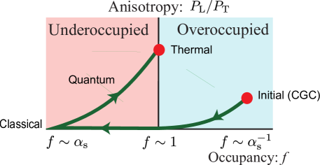
Figure 9: Schematic paths from the CGC-type initial condition to the thermalized state. Figure is adapted from a talk by Kurkela at Quark Matter 2015. (The original one plots $P_{\rm T}/P_{\rm L}$.)

According to the scenario in figure 9, $P_{\rm L}/P_{\rm T}$ initially decreases due to longitudinal expansion and it would go to the free-streaming limit unless the scattering effects are taken into account. It is the quantum effect incorporated in the collision terms that derives the system back to non-zero $P_{\rm L}/P_{\rm T}$ and eventually the system approaches a thermal state. It is actually a vital question what lets the system resist against the free-streaming limit, and there is not a consensus in the heavy-ion physics community yet, though the quantum fluctuations certainly play a key role.

Another profitable treatment of the collision term is to take the small angle limit assuming that massless gluon exchange is most enhanced there. Specifically, $t$- and $u$-channel terms in the $2\leftrightarrow 2$ scattering of (39) become dominant, and in this limiting situation the collision term takes an amazingly simple form [49], which has been developed in a context to address the question of the gluonic BEC formation speculated in [50]. We will discuss this possibility of the BEC formation in details in section 5 and we here take a quick look at the concrete form of the collision term. In [49] a variation of the QCD Boltzmann equation that behaves like a Fokker-Planck equation has been proposed with the collision term,

$$\biggl{(}\frac{\partial f(\boldsymbol{k})}{\partial t}\biggr{)}_{2\leftrightarrow 2}^{\theta\approx 0}=2\pi^{2}\alpha_{\rm s}^{2}\xi\boldsymbol{\nabla}_{k}\cdot\biggl{\{}I_{a}\boldsymbol{\nabla}_{k}f(\boldsymbol{k},t)+\hat{\boldsymbol{k}}I_{b}f(\boldsymbol{k},t)\bigl{[}1+f(\boldsymbol{k},t)\bigr{]}\biggr{\}}\;,$$ (41)

where $\boldsymbol{\nabla}_{k}\equiv\partial/\partial\boldsymbol{k}$. The overall factor $\xi$ is divergent and requires the UV and the IR cutoffs; $\xi\equiv(18/\pi)\int_{q_{\rm min}}^{q_{\rm max}}\rmd q/q$ with $q_{\rm max}\sim T$ and $q_{\rm min}\sim m_{\rm D}(\sim gT)$. Here, $I_{a}\equiv\int_{\boldsymbol{k}}f(\boldsymbol{k})[1+f(\boldsymbol{k})]$ and $I_{b}\equiv\int_{\boldsymbol{k}}2f(\boldsymbol{k})/|\boldsymbol{k}|\propto m_{\rm D}$. Obviously there is no resummation corresponding to the LPM effect since (41) corresponds to only $2\leftrightarrow 2$ scattering. Let us see some interesting properties of (41). First, we can easily check that the Bose-Einstein distribution function $f_{\rm eq}(\boldsymbol{k})$ leads to a relation, $I_{a}=TI_{b}$, so that (41) vanishes for $f_{\rm eq}(\boldsymbol{k})$ in equilibrium as it should. Second, the particle number obtained by the phase-space integral of $f(\boldsymbol{k},\boldsymbol{x})$ is conserved manifestly due to the fact that the right-hand side in (41) is a total derivative. Therefore, even though (41) looks very simple, it maintains the essence of the genuine $2\leftrightarrow 2$ collision term in (30). In the original discussions in [49] inelastic processes are turned off (apart from some qualitative remarks) and the gluon number is assumed to be a conserved quantity, which inevitably results in overpopulated gluons and an associated BEC formation. The effect of inelastic scattering has been later investigated and in a recent work [51] the splitting kernel is simplified into a form similar to the one in the RTA in (35). Regarding the BEC scenario and possible scaling solutions, more discussions will follow in section 5.

The fate of $P_{\rm L}/P_{\rm T}$ has been also extensively investigated not only in the dilute regime but also in the dense regime in terms of classical field simulations. In fact, when the occupation number becomes as large as $f\sim 1/\lambda$ in the $\lambda\phi^{4}$ theory or $f\sim 1/\alpha_{\rm s}$ in QCD, it is no longer legitimate to utilize the perturbation theory even for small coupling. In the dilute regime, usually, many-body scatterings like $m\leftrightarrow n$ processes are higher order with respect to the coupling constant. For example, a $3\leftrightarrow 3$ scattering in the $\lambda\phi^{4}$ is of order $\sim\lambda^{4}$ at the tree level, and the collision term involves five distribution functions, leading to the order of $\sim 1/\lambda$ in the saturated regime, which is of the same order as $2\leftrightarrow 2$ in (30). In this saturated regime we need to use a non-perturbative method such as the semi-classical approximation.

2.3.2 Dense regime — classical statistical simulation

The glasma instability was found in the purely classical simulation with $\delta\mathcal{A}^{\mu}(\tau,\nu\neq 0)$, and in the first simulation [40] the initial value of $\delta\mathcal{A}^{\mu}(\tau=\tau_{0},\nu)$ was treated as white noise proportional to some seed strength $\Delta$. For more quantitative studies, however, we should figure out what the realistic spectrum of $\Delta(\tau_{0},\nu)$ is. The first attempt along these lines is found in [52] based on an analogy to the harmonic oscillator problem in quantum mechanics.

It would give us some intuition if we consider the semi-classical approximation first not in quantum field theory but in quantum mechanics. Let us explain the idea with a simple example, which can be easily generalized later to quantum field theory problems. For a given density matrix $\hat{\rho}(t)$, the Wigner function is defined as

$$W(\boldsymbol{x},\boldsymbol{p};t)\equiv\frac{1}{(2\pi\hbar)^{3}}\int\rmd\delta\boldsymbol{x}\,\langle\boldsymbol{x}-{\textstyle\frac{1}{2}}\delta\boldsymbol{x}|\hat{\rho}(t)|\boldsymbol{x}+{\textstyle\frac{1}{2}}\delta\boldsymbol{x}\rangle\,\rme^{-\rmi\boldsymbol{p}\cdot\delta\boldsymbol{x}/\hbar}\;.$$ (42)

If $\hat{\rho}$ is a pure state of the one-dimensional harmonic oscillator ground state $|\psi_{0}\rangle$, and then the wave-function in the $x$ representation is a Gaussian; $\psi_{0}(x)\sim\exp(-x^{2}/2b^{2})$. It is then straightforward to confirm $W(x,p)\sim\exp(-x^{2}/b^{2}-b^{2}p^{2})$. Thus, roughly speaking, the Wigner function embodies a probability distribution for classical conjugate variables in a way consistent with the uncertainty principle. It should be mentioned, however, that the Wigner function as defined in (42) could take a negative value (usually when some quantum entanglement is involved), and so a naive interpretation as a probability distribution needs caution. It can be proved that a smeared Winger function (called the Husimi function) is always non-negative, which is a quite useful property to make a correspondence between the classical fields and the classical particle distributions [53].

From the von Neumann equation, $\rmi\hbar(\partial\hat{\rho}/\partial t)=[\hat{H},\hat{\rho}]$, the time evolution of the Wigner function is determined with the Moyal product as

$$\frac{\partial W(\boldsymbol{x},\boldsymbol{p};t)}{\partial t}=H(\boldsymbol{p},\boldsymbol{x})\,\frac{2}{\rmi\hbar}\,\sin\Bigl{[}\frac{\rmi\hbar}{2}\bigl{(}\overleftarrow{\partial_{\boldsymbol{p}}}\,\overrightarrow{\partial_{\boldsymbol{x}}}-\overleftarrow{\partial_{\boldsymbol{x}}}\,\overrightarrow{\partial_{\boldsymbol{p}}}\bigr{)}\Bigr{]}\,W(\boldsymbol{x},\boldsymbol{p};t)\;,$$ (43)

where the classical Hamiltonian appearing above reads:

$$H(\boldsymbol{x},\boldsymbol{p})=\int\rmd\delta\boldsymbol{x}\,\langle\boldsymbol{x}-{\textstyle\frac{1}{2}}\delta\boldsymbol{x}|\hat{H}|\boldsymbol{x}+{\textstyle\frac{1}{2}}\delta\boldsymbol{x}\rangle\,\rme^{-\rmi\boldsymbol{p}\cdot\delta\boldsymbol{x}/\hbar}\;.$$ (44)

We can then expand the above equation of motion in terms of $\hbar$ to find that, at the leading order, the time evolution is described by the classical equation of motion with the Poisson brackets:

$$\frac{W(\boldsymbol{x},\boldsymbol{p};t)}{\partial t}=\{H(\boldsymbol{p},\boldsymbol{x}),\,W(\boldsymbol{x},\boldsymbol{p},t)\}_{\rm P}+O(\hbar^{2})\;,$$ (45)

and there is no term of $O(\hbar)$. Therefore, at least at the $O(\hbar)$ accuracy, the initial Wigner function has all the quantum effects and the classical equations of motion remain intact. This observation is the theoretical foundation of the classical statistical simulation.

Historically, the classical statistical simulation has been developed in a wider context than the heavy-ion collision physics. A successful example in the thermalization problem in the Early Universe is found in [54] where turbulent behavior with self-similar dynamics has been observed in semi-classical $\lambda\phi^{4}$ theory (see also [55] for a more comprehensive report). On a more academic level, a scalar theory with high initial occupancy was considered in [56] to quantify classical aspects of real-time quantum dynamics, and the classical statistical formulation for non-Abelian gauge theories was given in [57]. There are fruitful outputs from the classical statistical simulation, especially many insightful indications about the fate of the isotropization (discussed more in section 3) and the weak wave turbulence in the pure Yang-Mills theory (discussed more in section 5). Interested readers are guided to the most recent review [58] on the classical statistical simulation.

For the rest of this subsubsection, let us explain how the initial Wigner function should be given for a special geometry in the heavy-ion collisions with longitudinal expansion. This problem was carefully resolved in [59] and further investigated for a scalar theory in [60] and for gauge field theories in [61]. Here, let us take a close look at the derivation of fluctuation spectrum in an expanding scalar theory defined with a Lagrangian density, $\mathcal{L}(\phi)=\frac{1}{2}(\partial^{\mu}\phi)^{2}-V(\phi)$. To mimic the glasma background, let us decompose a scalar field $\phi$ at small $\tau$ into an $\eta$-independent background $\varphi$ (which can be regarded as $\tau$-independent for $\tau\approx 0$) and $\eta$-dependent quantum fluctuations as

$$\phi(\boldsymbol{x}_{\perp},\eta,\tau\approx 0)=\varphi(\boldsymbol{x}_{\perp})+\frac{\sqrt{\pi}}{2}\int\frac{\rmd\nu}{2\pi}\rmd\mu_{K}\;\rme^{\pi\nu/2}\,c_{\nu K}\,\rme^{\rmi\nu\eta}\chi_{K}(\boldsymbol{x}_{\perp})H_{\rmi\nu}^{(2)}(\lambda_{K}\tau)+\mbox{c.c.}\;,$$ (46)

and the question is the probability distribution for the weight $c_{\nu K}$ of each mode. Here, $H_{\rmi\nu}^{(2)}(x)$ is the Hankel function and $\chi_{K}(\boldsymbol{x}_{\perp})$ represents the orthogonal basis function on top of the background $\varphi$, which is determined by the eigenvalue equation,

$$\bigl{[}-\boldsymbol{\nabla}_{\perp}^{2}+V^{\prime\prime}(\varphi)\bigr{]}\chi_{K}(\boldsymbol{x}_{\perp})=\lambda_{K}^{2}\,\chi_{K}(\boldsymbol{x}_{\perp})\;,$$ (47)

and $K$ is the quantum number to label different eigen-vectors. If the background potential $V^{\prime\prime}(\varphi)$ is spatially uniform, $K$ is nothing but a spatial momentum $\boldsymbol{k}$ and $\chi_{K}(\boldsymbol{x}_{\perp})$ is a plane wave. The choices of the eigen-function and the measure $\rmd\mu_{K}$ are not independent; a choice proposed in [60] is, using

$$\delta_{KK^{\prime}}\equiv\int\rmd^{2}\boldsymbol{x}_{\perp}\,\chi_{K}^{\ast}(\boldsymbol{x}_{\perp})\,\chi_{K^{\prime}}(\boldsymbol{x}_{\perp})\;,$$ (48)

the measure is normalized to satisfy,

$$\int\rmd\mu_{K}\,\delta_{KK^{\prime}}=1\;.$$ (49)

Then, the spectrum of initial quantum fluctuations is characterized in the following form:

$$\langle c_{\nu K}\,c_{\mu K^{\prime}}\rangle=0\;,\qquad\langle c_{\nu K}\,c_{\mu K^{\prime}}^{\ast}\rangle=\pi\delta(\nu-\mu)\delta_{KK^{\prime}}\;.$$ (50)

It might be a bit puzzling why (46) involves $H_{\rmi\nu}^{(2)}(\lambda_{K}\tau)$ even though we are interested only in the initial spectrum at $\tau=0^{+}$. The reason is that there are coordinate singularities at $\tau=0^{+}$ and for practical simulations we need to start the numerical simulation with some initial condition at small but finite $\tau$.

It is non-trivial how to define the occupation number from the classical fields. In other words, because the occupation number is an expectation value of the number operator in terms of the annihilation and the creation operators, what we need is the representation of the annihilation and the creation operators using the classical fields. This can be done with the projection to free particle basis, i.e. (see [62] for a related argument in the context of the Schwinger mechanism)

$$f_{\nu\boldsymbol{k}_{\perp}}(\tau)=-\frac{1}{2}+\frac{\pi\tau^{2}\rme^{\pi\nu}}{4S_{\perp}L_{\eta}}\biggl{\langle}\biggl{|}\int\rmd^{2}\boldsymbol{x}_{\perp}\rmd\eta\,\rme^{-\rmi\nu\eta-\rmi\boldsymbol{k}_{\perp}\cdot\boldsymbol{x}_{\perp}}\,H_{\rmi\nu}^{(2)\ast}(k_{\perp}\tau)\overset\leftrightarrow\partial\phi(\tau,\eta,\boldsymbol{x}_{\perp})\biggr{|}^{2}\biggr{\rangle}\;.$$ (51)

This formulation of the classical statistical simulation with correct quantum spectrum should reproduce at least the one-loop order results. The advantage lies in the stability for long time simulations, while serious shortcomings are found in the UV sector when applied for quantum field theories. First of all, the zero-point oscillation energy appears and it should be gotten rid of by some subtraction procedures. In ordinary quantum field theory the zero-point oscillation energy is just an offset in energy and safely discarded. The situation gets highly complicated as soon as inhomogeneous background fields are involved especially in expanding geometries. One prescription would be to take a finite difference between numerical results with and without the background fields, as was implemented in [63]. Secondly, the approximation in the classical statistical simulation may ruin the renormalizability of theory, which was shown perturbatively in [64].

To have a deeper insight into field theoretical problems inherent in the classical statistical simulation, it would be very useful to understand how the classical description can have a connection to the kinetic equation when the occupation number gets large. This question was formulated for $\lambda\phi^{4}$ theory in [65] and some subtleties in the derivation have been clarified in [66]. Here, let us take a quick look over the arguments in [65]. To make the question well-defined, we should work in a semi-saturated regime where $1\ll f\ll 1/\lambda$ is assumed.

The key elements are the real-time propagators $G_{ij}(x,y)$ in the so-called $ra$ basis. In non-equilibrium case the translational invariance could be violated and so, generally speaking, $G_{ij}(x,y)$ is a function of not only $\delta x=x-y$ but also $X=(x+y)/2$. Assuming that the $X$ dependence is slow, replacing $X$ with $x$, the Fourier transformed propagators with respect to $\delta x$ can be expressed as

$$\qquad G_{aa}(k,x) = 0\;,\quad G_{ra}(k,x)=\frac{\rmi}{k^{2}\!-\!m^{2}\!+\!\rmi\epsilon k_{0}}\;,\quad G_{ar}(k,x)=\frac{\rmi}{k^{2}\!-\!m^{2}\!-\!\rmi\epsilon k_{0}}\;,$$ (52)

$$\qquad G_{rr}(k,x) = \biggl{[}\frac{1}{2}+f(\boldsymbol{k},\boldsymbol{x},t)\biggr{]}\bigl{(}G_{ra}-G_{ar}\bigr{)}=\biggl{[}\frac{1}{2}+f(\boldsymbol{k},\boldsymbol{x},t)\biggr{]}\,2\pi\delta(k^{2}-m^{2})\;.$$ (53)

These propagators should satisfy the Dyson equation:

$$2\rmi k^{\mu}\partial_{\mu}G_{rr}(k,x)=G_{rr}(\Sigma_{ar}-\Sigma_{ra})+\Sigma_{aa}(G_{ar}-G_{ra})\;.$$ (54)

Because $f$ is large now, $G_{rr}(p,x)$ is dominant, and then the Dyson equation leads to a kinetic equation with the collision term in this approximation given by

$$\biggl{(}\frac{\partial f}{\partial t}\biggr{)}_{\rm coll}^{\rm classical}=\frac{-\rmi(\Sigma_{ar}-\Sigma_{ra})}{2k_{0}}\Bigl{(}f+\frac{1}{2}\Bigr{)}+\frac{\rmi\Sigma_{aa}}{2k_{0}}\;.$$ (55)

The self-energies can be computed according to the ordinary Feynman rule in the $\lambda\phi^{4}$ theory. Because all self-energies are written in terms of $G_{rr}\propto(1/2+f)$, we can understand that the collision term for the $2\leftrightarrow 2$ scattering is modified from the conventional form of (30) into

$$\biggl{(}\frac{\partial f(\boldsymbol{k}_{1})}{\partial t}\biggr{)}_{2\leftrightarrow 2}^{\rm classical}=\frac{\lambda^{2}}{4\omega(\boldsymbol{k}_{1})}\int_{\boldsymbol{k}_{2},\boldsymbol{k}_{3},\boldsymbol{k}_{4}}(2\pi)^{4}\delta^{(4)}(k_{1}+k_{2}-k_{3}-k_{4})\,$$

$$\quad\times\Bigl{\{}(f_{3}+{\textstyle\frac{1}{2}})(f_{4}+{\textstyle\frac{1}{2}})(f_{1}+{\textstyle\frac{1}{2}})+(f_{2}+{\textstyle\frac{1}{2}})(f_{3}+{\textstyle\frac{1}{2}})(f_{4}+{\textstyle\frac{1}{2}})$$

$$\qquad-(f_{1}+{\textstyle\frac{1}{2}})(f_{2}+{\textstyle\frac{1}{2}})(f_{3}+{\textstyle\frac{1}{2}})-(f_{4}+{\textstyle\frac{1}{2}})(f_{1}+{\textstyle\frac{1}{2}})(f_{2}+{\textstyle\frac{1}{2}})\Bigr{\}}\;,$$ (56)

where the cubic terms and the quadratic terms reproduce the correct ones in (30), while this above form has extra linear terms, $\propto f_{3}+f_{4}-f_{2}-f_{1}$. Surprisingly, the presence of these linear terms change the structure of theory in the UV region drastically [67]. To see this, let us consider the equilibrium distribution resulting from (56), that is easily found to be the Rayleigh-Jeans form:

$$f(\boldsymbol{k})\to\frac{T}{\omega(\boldsymbol{k})-\mu}-\frac{1}{2}\;,$$ (57)

which correctly reproduces first two terms from the expansion of the Bose-Einstein or Planck distribution. Therefore, this is a valid description for $f\gg 1$ with $\omega-\mu\ll T$. For large $|\boldsymbol{k}|$, however, $f(\boldsymbol{k})$ becomes smaller and smaller and eventually the approximation breaks down. In the genuine thermal equilibrium, $f(\boldsymbol{k})$ should have an exponential tail rather than a power-law decay, which cannot be reproduced in the semi-classical approximation.

This change to (57) is the clearest manifestation of the loss of renormalizability. In fact, with the distribution function (57), the total particle number and the energy are both UV divergent (i.e. UV catastrophe, which is a well recognized problem in the condensation of classical non-linear waves [68]) and a UV cutoff is necessary even though the underlying theory was originally renormalizable. This implies that the classical statistical simulation should suffer artificial dependence on a UV cutoff, which moreover affects the scaling behavior [69], as is the main subject in section 3.

2.4 Other Methods

It would be desirable to invent theoretical methods applicable to both dilute and dense regimes particularly to investigate the whole dynamics of an expanding system in the heavy-ion collision. There is unfortunately no such universal method so far, but theoretical attempts are making some progresses, some selected ones of which will be introduced in this section.

2.4.1 Kadanoff-Baym equations

The quantum upgraded version of the equations of motion is the Dyson-Schwinger equation. In principle the kinetic equation could be derived from the Dyson-Schwinger equation. It is still very difficult to solve the Dyson-Schwinger equation or similar functional equations in Minkowskian spacetime (see [70] for an attempt based on functional renormalization group equations); a part of subtlety comes from a technical difficulty in imposing a UV cutoff to Minkowskian four-vector. It would be a better strategy to transform the functional equation into a more convenient representation such as the 2PI formalism [71]. In the context of the real-time studies the 2PI formalism has been successful for the $1/N$ expansion in $O(N)$ scalar theories as discussed diagrammatically in [72] and numerically with instability in [73].

The 2PI effective action (for a bosonic field) reads:

$$\Gamma[G]=\frac{\rmi}{2}\Tr_{C}\bigl{[}\ln G^{-1}+G_{0}^{-1}G\bigr{]}+\Gamma_{2}[G]\;,$$ (58)

where $G_{0}$ and $G$ represent the free and the full propagators, respectively, and $\Gamma_{2}[G]$ is the contribution from 2PI diagrams in terms of bare vertices and full propagators. The trace $\Tr_{C}$ is taken along the closed-time path. The full propagator and the self-energy are determined functionally from stationary conditions,

$$\frac{\delta\Gamma[G]}{\delta G}=0\;,\qquad\Pi=2\rmi\frac{\delta\Gamma_{2}[G]}{\delta G}\;,$$ (59)

which yield the Kadanoff-Baym equations. The propagator and the self-energy are decomposed into statistical and spectral parts; $G(x,y)=G_{F}(x,y)-\frac{\rmi}{2}{\rm sign}_{C}(x^{0}-y^{0})G_{\rho}(x,y)$ and $\Pi(x,y)=-\rmi\delta_{C}(x-y)\Pi^{\rm(local)}(x)+\Pi_{F}(x,y)-\frac{\rmi}{2}{\rm sign}_{C}(x^{0}-y^{0})\Pi_{\rho}(x,y)$, where ${\rm sign}_{C}(x^{0}-y^{0})\equiv\Theta_{C}(x^{0}-y^{0})-\Theta_{C}(y^{0}-x^{0})$. The Kadanoff-Baym equations read [74]:

$$\bigl{[}\partial^{2}+M^{2}(x)\bigr{]}G_{F}(x,y)=\int_{0}^{y^{0}}\rmd^{4}z\,\Pi_{F}(x,z)G_{\rho}(z,y)-\int_{0}^{x^{0}}\rmd^{4}z\,\Pi_{\rho}(x,z)G_{F}(z,y)\;.$$ (60)

$$\bigl{[}\partial^{2}+M^{2}(x)\bigr{]}G_{\rho}(x,y)=-\int_{y^{0}}^{x^{0}}\rmd^{4}z\,\Pi_{\rho}(x,z)G_{\rho}(z,y)$$ (61)

with $M^{2}(x)\equiv m^{2}+\Pi^{\rm(local)}(x)$. The Wigner transformed propagators are defined as $\tilde{G}_{F}(X,k)=\int\rmd^{4}\delta x\,\rme^{\rmi k\delta x}G_{F}(X+\frac{\delta x}{2},X-\frac{\delta x}{2})$ and $\tilde{G}_{\rho}(X,k)=-\rmi\int\rmd^{4}\delta x\,\rme^{\rmi k\delta x}G_{\rho}(X+\frac{\delta x}{2},X-\frac{\delta x}{2})$. The gradient expansion leads to a Boltzmann-type kinetic equation for the distribution function $f(X,k)$ where it is defined from $\tilde{G}_{F}=\tilde{G}_{\rho}(f+\frac{1}{2})$ and the quasi-particle approximation, $\tilde{G}_{\rho}=\pi\bigl{[}\delta(k^{0}-\varepsilon(X,\boldsymbol{k}))-\delta(k^{0}+\varepsilon(X,\boldsymbol{k}))\bigr{]}/\varepsilon(X,\boldsymbol{k})$ with $\varepsilon(X,\boldsymbol{k})=\sqrt{\boldsymbol{k}^{2}+M^{2}(x)}$, is used.

A qualitative difference between the Boltzmann equation and the Kadanoff-Baym equation appears from the quasi-particle approximation, without which the collision phase space opens for $0\leftrightarrow 4$, $1\leftrightarrow 3$, $2\leftrightarrow 2$ off-shell processes in the $\lambda\phi^{4}$ theory. The numerical simulation of the QCD Kadanoff-Baym equation is still an ambitious challenge. To simplify the treatment of the spectral function, $\tilde{G}_{\rho}$, a Lorentzian Ansatz was introduced in some phenomenological approaches (see [75] for a review), and the more full self-consistent treatment was carried out in [76] with the aim to make a unified formalism with the CGC background. This direction of research should deserve more studies with computer resource invested in the future.

2.4.2 Stochastic quantization

The Monte-Carlo integration is useless when the sign problem is severe, and this is why the direct QCD simulation is so difficult in Minkowskian spacetime. Then, one idea to overcome the sign problem is to quantize a field theory in a different way, using a Langevin equation, which is conceivable because quantum effects are fluctuations around the classical paths. One of the oldest attempts along these lines is the derivation of the Schrödinger equation from a Brownian motion by Nelson [77]. It is known that classical noises are inadequate for correct quantization, but it is possible to reformulate the quantization procedure by adding a fictitious time or a quantum axis. This method is thus an example of the so-called holographic principle that states an equivalence between $D$-dimensional quantum theory and $(D+1)$-dimensional classical theory.

A complete review is available in [78]; here, we simply sketch the idea. For a simple scalar theory, the Langevin equation to describe the evolution with the fictitious time $\theta$ is written down as

$$\partial_{\theta}\phi(x,\theta)=\rmi\frac{\delta S}{\delta\phi(x)}\biggr{|}_{\phi(x)\to\phi(x,\theta)}+\eta(x,\theta)\;,$$ (62)

where $S$ is an action to define the theory and $\eta(x,\theta)$ is a stochastic noise satisfying $\langle\eta(x,\theta)\eta(x^{\prime},\theta^{\prime})\rangle_{\eta}=2\delta^{(4)}(x-x^{\prime})\delta(\theta-\theta^{\prime})$. It is claimed that the quantum expectation value of an operator $\mathcal{O}[\phi(x)]$ is given by

$$\langle\mathcal{O}[\phi(x)]\rangle=\lim_{\theta\to\infty}\langle\mathcal{O}[\phi(x,\theta)]\rangle_{\eta}\;.$$ (63)

Using the stochastic diagrams, we can map the above procedures faithfully to the conventional Feynman diagrams. Therefore, the perturbative equivalence has no doubt based on diagrammatic considerations, while the non-perturbative simulations could violate this perturbative equivalence.

Because the Langevin equation in (62) is complex with an imaginary unit in front of the drift term, this quantization procedure is nowadays called the complex Langevin method. The first successful report on the real-time quantization is [79], in which the boundary condition was not correctly implemented, and a more refined simulation was performed in [80]. The method seemed to be promising apart from a stability problem in a long-time simulation. Later, the real-time complex Langevin method was revisited in [81] and it was found that the numerical simulation has a general tendency to fall into a wrong answer.

New insights to the complex Langevin method have emerged from careful analyses in comparison to the Lefschetz thimble method that looks similar to the complex Langevin method but has a firm mathematical foundation. The relation between these two methods has been understood numerically [82] and analytically [83], which was useful to clarify the origin of the convergence problem in the complex Langevin method. In general, when the Stokes phenomenon occurs in complexified theories, the convergence becomes subtle, which can be understood from phase factors of distinct Lefschetz thimbles [84]. Usually the Stokes phenomenon corresponds to a phase transition in equilibrium environments and so the complex Langevin method works poorly only when the system approaches a phase transition [85]. In Minkowskian spacetime the situation is much worse and the onset of the Stokes phenomenon is found around the on-shell conditions, and the validity region is tightly limited. Without some breakthrough, it is unlikely that the complex Langevin method or the Lefschetz thimble method can capture the correct real-time dynamics of interested physics problems. An important lesson that we can learn is that some unexpected complication may appear and a different prescription to quantize a theory may change non-perturbative contents of the theory, which could be understood from a well-known mathematical fact that many inequivalent functions can happen to have identical asymptotic series.

2.4.3 Gauge/gravity correspondence

The most widely recognized example of the holographic principle is the correspondence between the gauge theory and the gravity theory, i.e., the $\mathcal{N}=4$ supersymmetric Yang-Mills theory in the large-$N_{\rm c}$ limit and the classical solution (anti-de Sitter; AdS₅ metric) of the super-gravity theory. In the heavy-ion community this method has become very popular since the successful calculation of the shear viscosity [86].

The key relation of the correspondence is summarized in a form of the GKP-Witten relation;

$$\biggl{\langle}\exp\biggl{[}\rmi\int\rmd^{4}x\,\phi_{0}(x)\mathcal{O}(x)\biggr{]}\biggr{\rangle}=\rme^{\rmi S_{\tiny\mbox{gravity}}[\phi_{0}(x)]}\;,$$ (64)

where the left-hand side is the expectation value in gauge field theory and the right-hand side is the on-shell action in the classical gravity theory with the boundary condition $\phi\to\phi_{0}$ at the boundary. Apart from decoupled and irrelevant coordinates in $S^{5}$, the fifth coordinate $z$ in addition to Minkowskian $t$ and $\boldsymbol{x}$ refers to the quantum axis, which together span AdS₅ space. In the gravity side the theory is described by the equations of motion in a bulk from $z=\infty$ (UV) toward $z=0$ (IR) and the gauge theory resides in a boundary at $z=0$; in this sense, the gauge/gravity correspondence could be regarded as the bulk/boundary correspondence or the UV/IR correspondence.

The very first application of the gauge/gravity correspondence to investigate the early-time dynamics in the heavy-ion collision is a work by Janik and Peschanski in [87], which was re-derived also in [88]. For a pedagogical introduction, a review by Peschanski [89] should be quite readable for “users” of this string-inspired technique.

Like the lattice-QCD simulation, the gauge/gravity correspondence is a powerful method to compute an expectation value of gauge invariant operator, and for the early-time dynamics in the heavy-ion collision, the most informative observable is the energy-momentum tensor $T_{\mu\nu}$. What we should do first is to obtain the solution of the 5-dimensional gravity equations as $\rmd s^{2}=[g_{\mu\nu}(z)\rmd x^{\mu}\rmd x^{\nu}+\rmd z^{2}]/z^{2}$ in the Fefferman-Graham form (choosing appropriate coordinates). Then, the energy-momentum tensor is inferred from the relation,

$$g_{\mu\nu}(z\approx 0,x)=\eta_{\mu\nu}+\frac{2\pi^{2}}{N_{\rm c}^{2}}\langle T_{\mu\nu}(x)\rangle\,z^{4}+\cdots\;.$$ (65)

In [87, 88] a black-hole solution has been discovered that corresponds to the one-dimensional expansion of hydrodynamics (i.e. the Bjorken solution). The most interesting finding is that the time dependence of the energy density $\varepsilon(\tau)$ is a constant initially and turns to $\tau^{-4/3}$ later; this latter scaling recovers the fully isotropized hydrodynamical one in (37). The transitional change from a constant to $\tau^{-4/3}$ behavior should be identified as the isotropization point, which yields an isotropization time scale as

$$\tau_{\rm iso}=\biggl{(}\frac{3N_{\rm c}^{2}}{2\pi^{2}e_{0}}\biggr{)}^{3/8}\;,$$ (66)

where $e_{0}$ is defined through the initial energy density $\varepsilon_{0}=e_{0}\tau_{0}^{4/3}$ at $\tau=\tau_{0}$. If we consider $\varepsilon_{0}\sim 15\,\mbox{GeV}/\,\mbox{fm}^{3}$ at $\tau_{0}=0.6\,\mbox{fm}/c$ at RHIC energy, we can have an estimate at strong coupling as $\tau_{\rm iso}\simeq 0.3\,\mbox{fm}/c$, which might be an account for the fast isotropization.

Instead of postulating a black hole solution corresponding to dynamical QGP, the heavy-ion collision itself could be emulated by a shock-wave collision in the gravity side, which looks like a CGC-like problem to solve the classical equations of motion with two colliding sources (and like the CGC setup the one shock-wave problem is analytical solvable; see a pedagogical review [90] and references therein). The pioneering numerical work to simulate the horizon (and QGP in a gauge dual side) formation is found in [91], in which $P_{\rm T}$ and $P_{\rm L}$ have been calculated as functions of time. Interestingly, right after the collision, $P_{\rm T}$ goes positively and $P_{\rm L}$ goes negatively, in a way similar to the CGC simulation. This implies that a picture of extending color flux tubes in the CGC initial condition should be the right physics description for the very early dynamics. However, in the gauge/gravity numerical simulation, it has been observed that $P_{\rm L}/P_{\rm T}\to 1$ as quickly as $\tau_{\rm iso}\sim 0.7/T\simeq 0.5\,\mbox{fm}/c$ for the initial temperature $T\sim 0.35\,\mbox{GeV}$. Later, in [92], by means of the holographic numerical solutions, the validity of (first-order) viscous hydrodynamics has been tested in a region where $P_{\rm L}/P_{\rm T}<1$, which was such an important test that the way of thinking in the heavy-ion community was changed. Before [92], there were many studies on the isotropization, and sometimes it was not clearly distinguished from the hydrodynamization. Now, we know that the viscous hydrodynamics can work well even when strong anisotropy still remains. It might sound a bit puzzling that the viscous hydrodynamics is required for the system described by a gauge/gravity dual in which the shear viscosity is as small as the unitarity limit and the bulk viscosity is vanishing. We will come back to this question in section 4.

3 More on Isotropization

This section is devoted to a status summary of the scaling solution and its classification that includes a possibility going to the free-streaming limit. It is still under dispute what microscopic dynamics can sustain the system staying away from the vanishing longitudinal pressure.

3.1 Scaling Properties

To sort various scenarios out, it is quite useful to introduce a scaling form of the solution for the gluon distribution as a function of time. The self-similarity that has been confirmed in many classical statistical simulations implies the following scaling properties for the gluon distribution:

$$f(\boldsymbol{k},\tau)=(Q_{\rm s}\tau)^{\alpha}f_{\rm S}\bigl{(}(Q_{\rm s}\tau)^{\beta}k_{\perp},(Q_{\rm s}\tau)^{\gamma}k_{z}\bigr{)}\;,$$ (67)

which was systematically studied in [93] (which nicely reviews all technical details including lattice discretization). The exponents $\alpha$, $\beta$, and $\gamma$ characterize the non-equilibrium dynamical evolution, and these are reminiscent of the critical exponents in the vicinity of IR fixed points on the renormalization flow. This is a new form of the universality out of equilibrium, and unlike the static situation, there is no simple classification of the universality class only according to the dimensionality and the global symmetry.

Authors	$\alpha$	$\beta$	$\gamma$
BMSS [32]	$-2/3$	$0$	$1/3$
B [94]	$-3/4$	$0$	$1/4$
BGLMV [50]	$-(3-\delta_{s})/7$	$(1+2\delta_{s})/7$	$(1+2\delta_{s})/7$
KM [95]	$-7/8$	$0$	$1/8$

Table 1: Different exponents according to different scenarios with one-dimensional expansion. If complete thermalization with isotropy is achieved, $\alpha=0$, $\beta=\gamma=1/3$ should be realized.

In the case with one-dimensional expansion, a typical value of $k_{z}$ should be decreased as $\tau$ elapses, so that $\gamma$ is supposed to be positive. In fact, in the free-streaming limit, $\gamma=1$ is expected. Quantitative values of $\alpha$, $\beta$, and $\gamma$ strongly depend on the interactions or the collision terms in the Boltzmann equation. Table 1 is a list of exponents with one-dimensional expansion as discussed in [93]. Here, we will not see all the derivations, but focus on the value of BMSS which refers to the bottom-up thermalization scenario in [32].

As explained in section 2.2 $\Delta k_{\perp}^{2}$ was estimated by $\hat{q}\sim\alpha_{\rm s}^{2}T^{3}$ in the bottom-up thermalization. To identify the scaling exponent, we must know how $\hat{q}$ should parametrically depend on the distribution function; that is, $\hat{q}\sim\int\rmd^{2}k_{\perp}\,k_{\perp}^{2}\,\rmd\Gamma/\rmd^{2}k_{\perp}$ where $\rmd\Gamma/\rmd^{2}k_{\perp}$ is the scattering rate that scales as $\sim\alpha_{\rm s}^{2}\int\rmd k_{z}\,f^{2}$, and eventually we have $\hat{q}\sim\alpha_{\rm s}^{2}\int_{\boldsymbol{k}}f^{2}\sim(Q_{\rm s}\tau)^{2\alpha-2\beta-\gamma}$. Because $\hat{q}\sim\Delta k_{\perp}^{2}/\rmd\tau$, it is conceivable to postulate the collision term parametrically scaling as $(\partial f/\partial\tau)_{\rm coll}\sim(\Delta k_{\perp}^{2}/\rmd\tau)\cdot(\partial f/\Delta k^{2})\sim\hat{q}\partial_{p_{z}}^{2}f\sim(Q_{\rm s}\tau)^{3\alpha-2\beta+\gamma}$, where the small angle approximation was used to pick only $\partial_{p_{z}}$ up from $\nabla_{p}$ [see also (41)]. From the Boltzmann equation (33), we can immediately deduce $\rmd f/\rmd\tau\sim(Q_{\rm s}\tau)^{\alpha-1}\sim(Q_{\rm s}\tau)^{3\alpha-2\beta+\gamma}$, leading to

$$2\alpha-2\beta+\gamma=-1\;.$$ (68)

As long as the elastic collision is dominant, which is the case for the scattering processes with $k_{\rm br}\sim Q_{\rm s}$, the gluon number is approximately a conserved quantity. This gives, in the one-dimensional expanding geometry, $\mbox{(const)}\sim(Q_{\rm s}\tau)\int_{\boldsymbol{k}}f\sim(Q_{\rm s}\tau)^{\alpha-2\beta-\gamma+1}$. In the same way, the energy conservation gives another scaling relation. With an energy quanta approximated as $\omega(\boldsymbol{k})\sim k_{\perp}$, which is true for $\gamma>\beta$ in late time, it is straightforward to see that the energy conservation and the momentum conservation can be simultaneously satisfied only when $k_{\perp}\sim\mbox{(const)}$, i.e., $\beta=0$. Therefore, we have two more conditions as

$$\alpha-2\beta-\gamma=-1\;,\qquad\beta=0\;.$$ (69)

Here, we should note that the number conservation is a robust argument as long as elastic scatterings are dominant, while the energy conservation is not. An immediate counter example is the full thermalized system for which $\alpha=0$, $\beta=\gamma=1/3$ should be expected, which seems to violate the energy conservation. In fact, the energy is lost by the expansion with non-zero longitudinal pressure, and thus, the above scaling arguments implicitly assume a situation close to the free-streaming limit. With these cautions in mind, we can solve these scaling relations to determine the exponents uniquely as $\alpha=-2/3$ and $\gamma=1/3$, and this is how BMSS values in table 1 are obtained.

It is interesting to point out that BMSS, B, and KM satisfy (69), which means that the total particle number and the energy are strictly conserved and the difference in the exponents is attributed to the concrete form of the collision terms; namely, (68) may be changed by various scenarios. Indeed, if the collision term has another scaling; $(\partial f/\partial\tau)_{\rm coll}\sim(Q_{\rm s}\tau)^{\mu}$, then (68) should be replaced with $\mu-\alpha=-1$.

Now, a question may well arise from the exception in table 1; what is assumed in BGLMV that obviously violates either particle number or energy conservation. Because we can confirm that $\alpha-3\beta-\gamma=-1$ holds apart from $\delta_{s}$ that represents the effect of expansion, the energy is conserved in this scenario, while the particle number conservation is abandoned. Actually, this scenario accommodates a possibility of the BEC formation and a finite fraction of particles condenses at the zero mode. We discuss this speculative picture in details in section 5.

The classical statistical simulation in the pure Yang-Mills theory favors the BMSS exponents according to the results in [93]. This idea of the universality classification based on the scaling properties could open a new theoretical scheme to tackle non-equilibrium statistical physics in general [96] and it would be a challenging problem to establish a complete list of classification, i.e., a counterpart of the classification of the dynamical critical phenomena as summarized in [97]. For our purpose of the isotropization problem in the heavy-ion collision, though a deviation from $\gamma=1$ certainly suggests non-trivial physics different from the free-streaming limit, $P_{\rm L}/P_{\rm T}$ goes vanishingly small for large $\tau$ as long as the scaling (67) with $\gamma>\beta$ is the case.

3.2 Classical vs. Quantum Simulations

The most relevant quantity of our interest in the heavy-ion collision is the time-dependence of $P_{\rm L}/P_{\rm T}$, and it would make sense to parametrize it as $P_{\rm L}/P_{\rm T}\sim(Q_{\rm s}\tau)^{-\beta_{\rm eff}}$, or equivalently,

$$\beta_{\rm eff}\equiv-\tau\frac{\rmd}{\rmd\tau}\ln(P_{\rm L}/P_{\rm T})\;,$$ (70)

which is an exponent introduced in [69]. Because the longitudinal/transverse pressure is to be written as $P_{\rm L/T}(\tau)=\int_{\boldsymbol{k}}(k_{\parallel/\perp}^{2}/(2)|\boldsymbol{k}|)f(\boldsymbol{k},\tau)$, we see $\beta_{\rm eff}\sim 2(\gamma-\beta)$, which goes to $\beta_{\rm eff}\to 2$ in the free-streaming limit ($\beta=0$ and $\gamma=1$) and $\beta_{\rm eff}\to 2/3$ in the classical statistical simulation or in BMSS ($\beta=0$ and $\gamma=1/3$), and supposedly in realistic physical systems $\beta_{\rm eff}\to 0$ should be the right answer. Thus, we can rephrase the isotropization problem as a puzzle to explain $\beta_{\rm eff}=0$ that has never been realized in reliable numerical simulations.

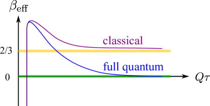
Figure 10: Schematic picture of the evolution of the exponent characterizing the isotropization degree. Figure sketched based on the results in [69].

A profound insight has been gained in a comparison between results with full quantum interactions and classical truncations using the Boltzmann equation for $\lambda\phi^{4}$ theory [69]. As explained in the last part in section 2.3.2, when $f\gg 1$, the cubic term $\sim f^{3}$ should be dominant among the collision terms in the $2\leftrightarrow 2$ processes. Such an approximation to truncate the collision terms to keep $\sim f^{3}$ only and discard $\sim f^{2}$ should correspond to the approximation employed in the classical statistical simulation. It is therefore intriguing to confirm numerically $\beta_{\rm eff}\to 0$ from the quantum Boltzmann equation and $\beta_{\rm eff}\to 2/3$ from the classical truncations. The practically important question is, in particular, whether $\beta_{\rm eff}\simeq 0$ could be realized even transiently or not in the classical approximation, and if the results are affirmative, there may be still a good chance to utilize the semi-classical approximation to resolve the isotropization problem. The numerical results are summarized in an illustration in figure 10. It is a striking feature that the semi-classical results monotonically converge to the so-called classical attractor with $\beta_{\rm eff}=2/3$ and does not come close to $\beta_{\rm eff}\sim 0$ at all. As a matter of fact, figure 10 is an apparently different but equivalent representation of the sketch in figure 9.

It is thus an urgent problem in theory to pursue for some interpolating description used from the dilute to the dense regimes. Especially in the dense regime, $f\gg 1$ does not hold for all the momenta, and so the conventional methods are inadequate for the large momentum regions. So far, it remains as a tough open question how to improve the theoretical formulation in the dense regime extrapolatably toward the dilute regime.

4 More on Onset of Hydrodynamics

It would be a reasonable question to wonder what would happen if the hydrodynamic equations are forcefully employed when $P_{\rm L}\ll P_{\rm T}$. If the usage of the hydrodynamic equations were legitimate even with anisotropic pressures, we do not have to try to isotropize the system using the plasma/glasma instabilities but simply switch to hydrodynamics immediately after the glasma initial condition. In an ordinary sense, anisotropic pressures are accompanied by dissipative terms and if the anisotropy is large such that the derivative expansion can no longer be justified, we should not utilize the hydrodynamic equations. Recently, however, a promising project for resummed anisotropic hydrodynamic is ongoing under the name of the aHydro [98, 99]. This section is devoted to a brief summary of this interesting and still developing subject.

4.1 Basics of Hydrodynamics

Here, we would not attempt to elucidate the systematic derivation of the hydrodynamic equations, but instead, we just take a quick look at some basic expressions which are later necessary for the understanding of the effect of anisotropic pressures.

We follow the discussions in [100]. The starting point for hydrodynamics is the energy and the momentum conservation laws expressed in terms of the energy-momentum tensor as

$$\partial_{\mu}T^{\mu\nu}=0\;.$$ (71)

If there are some conserved charges such as the electric charge and the baryon number, the continuity equation for such quantities should be coupled, which we neglect in this subsection for simplicity. The fundamental variable for the hydrodynamic description is the velocity vector $u^{\mu}$ which is normalized as $u_{\mu}u^{\mu}=1$. Then, the energy momentum tensor can be decomposed as

$$T^{\mu\nu}=\varepsilon u^{\mu}u^{\nu}-(P+\Pi)\Delta^{\mu\nu}+W^{\mu}u^{\nu}+W^{\nu}u^{\mu}+\pi^{\mu\nu}\;,$$ (72)

where $\Delta^{\mu\nu}\equiv g^{\mu\nu}-u^{\mu}u^{\nu}$. The physical interpretation of each term is quite clear; $\varepsilon$ is the energy density, $P+\Pi$ is the pressure, $W^{\mu}$ is the energy flow, and $\pi^{\mu\nu}$ is the viscous stress tensor, which is defined by $\pi^{\mu\nu}=T^{\langle\mu\nu\rangle}\equiv\Delta^{\mu\nu}_{\;\;\alpha\beta}T^{\alpha\beta}$, where

$$\Delta^{\mu\nu\alpha\beta}\equiv\frac{1}{2}(\Delta^{\mu\alpha}\Delta^{\nu\beta}+\Delta^{\nu\alpha}\Delta^{\mu\beta})-\frac{1}{3}\Delta^{\mu\nu}\Delta^{\alpha\beta}\;.$$ (73)

It is easy to show that $\Delta^{\mu}_{\;\mu\alpha\beta}=0$, from which $\pi^{\mu}_{\;\mu}=0$ follows. Because $u_{\mu}\Delta^{\mu\nu}=0$ by definition, we easily see $u_{\mu}\pi^{\mu\nu}=0$. For the hydrodynamic description we further need specify the choice of $u^{\mu}$; in other words, we are supposed to choose which conserved quantity flows with $u^{\mu}$. For the relativistic theory the energy current would be the most convenient choice, so that $T^{\mu}_{\;\nu}u^{\nu}=\varepsilon u^{\mu}$ follows. Such a frame in which $u^{\mu}$ represents the energy current is often called the Landau frame. In this frame, $W^{\mu}=0$ simplifies the structure of the energy-momentum tensor a bit and we should still need solve $\Pi$ and $\pi^{\mu\nu}$.

These continuity equations do not form a closed set of equations and more unknown variables are contained in $\Pi$ and $\pi^{\mu\nu}$ than equations even with an additional constraint from the equation of state, $P=P(\varepsilon)$, given from thermodynamics. To find an explicit form of $\Pi$ and $\pi^{\mu\nu}$, a phenomenological argument makes use of the 2nd-law of thermodynamics (see [101] for more field theoretical derivation of relativistic hydrodynamics), i.e. $\partial_{\mu}s^{\mu}\geq 0$ for a given entropy current $s^{\mu}$. The entropy current could be expressed as

$$s^{\mu}=\frac{1}{T}T^{\mu\nu}u_{\nu}+\frac{p}{T}u^{\mu}+Q^{\mu}\;,$$ (74)

where the last term $Q^{\mu}$ represents 2nd-order dissipative terms that are not taken into account in the 1st-order viscous hydrodynamics. In the 1st-order theory the divergence of the entropy current turns out to be

$$T\partial_{\mu}s^{\mu}=-\Pi\cdot\nabla_{\mu}u^{\mu}+\pi_{\mu\nu}\cdot\partial^{\langle\mu}u^{\nu\rangle}\;,$$ (75)

where $\nabla_{\mu}\equiv\Delta_{\mu\nu}\partial^{\nu}$. To satisfy $\partial_{\mu}s^{\mu}\geq 0$, it would be sufficient to require that $\partial_{\mu}s^{\mu}$ is a sum of squared quantities, which immediately leads to

$$\Pi=-\zeta\nabla_{\mu}u^{\mu}\;,\qquad\pi^{\mu\nu}=2\eta\,\partial^{\langle\mu}u^{\nu\rangle}$$ (76)

with some positive coefficients, $\zeta$ and $\eta$, which are called the bulk and the shear viscosities, respectively. These transport coefficients should be given as inputs (from the linear-response theory, for example) to viscous hydrodynamics.

This framework of the 1st-order hydrodynamic equations has a serious flaw violating the causality. The problem can be cure by the 2nd-order theory that incorporates neglected $Q^{\mu}$; we can obtain $Q^{\mu}$ in terms of $u^{\mu}$, $\Pi$, and $\pi^{\mu\nu}$, and the condition for $\partial_{\mu}s^{\mu}$ involves their time derivatives, so that (76) should be replaced with the equations of motion for $\Pi$ and $\pi^{\mu\nu}$ with more transport coefficients, namely, the relaxation times, $\tau_{\Pi}$ for $\Pi$ and $\tau_{\pi}$ for $\pi^{\mu\nu}$. If these relaxation times are large enough, there is no problem to violate the causality.

It would be useful to write some of the explicit equations down here in a special case corresponding to the heavy-ion collision as addressed in [102]. Let us focus on the boost-invariant and conformal case and then we can drop the bulk viscosity effect. We can then simplify the 2nd-order viscous equations significantly as

$$\frac{\rmd\varepsilon}{\rmd\tau}+\frac{\varepsilon+P}{\tau}=\frac{\Phi}{\tau}\;,$$ (77)

where $\Phi\equiv\pi^{00}-\pi^{zz}$. (In [102] there was a factor $2/3$ error, which was corrected in an erratum.) Also, there is an equation to determine $\Phi$ that reads:

$$\frac{\rmd\Phi}{\rmd\tau}=-\frac{\Phi}{\tau_{\pi}}-\frac{\Phi}{2}\biggl{[}\frac{1}{\tau}+\frac{T}{\beta_{2}}\frac{\rmd}{\rmd\tau}\biggl{(}\frac{\beta_{2}}{T}\biggr{)}\biggr{]}+\frac{2}{3\beta_{2}\tau}$$ (78)

with $\beta_{2}=\tau_{\pi}/(2\eta)$. This equation can be further simplified with the conformality assumption in which $\beta_{2}\propto T^{-4}$ and we can use $T\propto\tau^{-1/3}$ for the term proportional to $\Phi/\beta_{2}$ in the construction of the 2nd-order theory. Then, the $\tau$ derivative gives a factor $5/3$, and we eventually have,

$$\frac{\rmd\Phi}{\rmd\tau}=-\frac{\Phi}{\tau_{\pi}}-\frac{4\Phi}{3\tau}+\frac{4\eta}{3\tau_{\pi}\tau}\;.$$ (79)

These are simple but useful equations for the benchmark purpose. Any extension of the hydrodynamic equations with resummation with respect to anisotropy should reproduce them once expanded in terms of small anisotropy, which will be checked later.

4.2 Dissipative Terms and Anisotropy

The ordinary hydrodynamic equations have only single $P$ assuming isotropy. The tensor decomposition in (72) suggests that $P_{\rm L}\neq P_{\rm T}$ could be related to some dissipative terms from $\pi^{\mu\nu}$, and this is indeed true. Therefore, if we improve hydrodynamics from the 1st-order theory to the 2nd-order theory, we may have a better situation to treat a larger deviation of $P_{\rm L}/P_{\rm T}\neq 1$, but eventually, we need reorganize the derivative expansion shifting the expansion reference point. In general circumstances such reorganization is a tough problem but the kinetic equation can provide us with a useful guide to the right path.

4.2.1 Hydrodynamic interpretation of anisotropy

Interestingly, (77) is a hydrodynamic counterpart of (38). We note that (38) is an exact relation regardless of hydrodynamics, and this means that, by taking a difference between (38) and (77), we have $P-\Phi=P_{\rm L}$. We here assume that $P$ appearing in the previous subsection is identifiable to an average; $(2P_{\rm T}+P_{\rm L})/3$. Also, in the 1st-order theory, $\tau_{\pi}\to 0$, and this implies that two terms in (79) should cancel, leading to a relation; $\Phi=4\eta/(3\tau)$ [102]. Combining these relations, we finally reach the following;

$$P_{\rm T}-P_{\rm L}=\frac{3}{2}\Phi=\frac{2\eta}{\tau}\;.$$ (80)

This clearly shows that $P_{\rm L}/P_{\rm T}\neq 1$ should be accompanied by a shear viscosity, and if it substantially remains constant at later time, it would favor a large value of the shear viscosity, while $\eta$ could be small for small $\tau$. In fact, in the classical statistical simulation with $P_{\rm L}/P_{\rm T}\sim 0.6$ the viscosity to the entropy density ratio was estimated in this way and the result was $\eta/s\sim 0.3$ [63], which is much smaller than the perturbative estimate (for the coupling $g=0.5$ that was adopted in the numerical simulation).

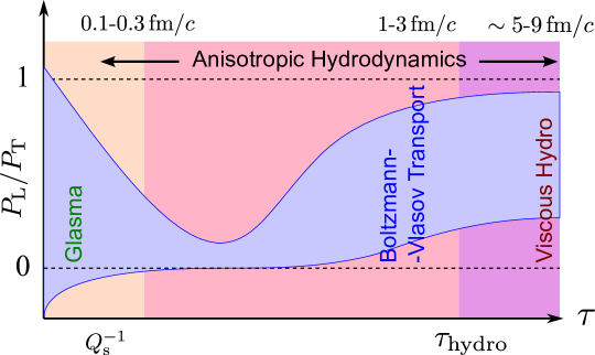
Figure 11: Schematic picture of the evolution of $P_{\rm L}/P_{\rm T}$ and the hydrodynamization time $\tau_{\rm hydro}$ which can be taken to be smaller once the hydrodynamic equations are augmented with large anisotropic effects. Figure adapted from a talk by Strickland.

We can equivalently rewrite (80), using $s\sim\partial P/\partial T\sim 4P/T$, into a form of the ratio as follows:

$$\frac{P_{\rm L}}{P_{\rm T}}=\frac{3\tau T-16(\eta/s)}{3\tau T+8(\eta/s)}\;,$$ (81)

which implies $P_{\rm L}/P_{\rm T}\approx 0.5$ for initial $\tau_{0}\sim 0.5\,\mbox{fm}/c$ and $T_{0}\sim 0.4\,\mbox{GeV}$, if $\eta/s\sim 1/(4\pi)$ is assumed, at RHIC energy. The reduction of $P_{\rm L}/P_{\rm T}$ suggested by (80) or (81) gives us a motive to pursue for an improved hydrodynamic formulation that can incorporate $P_{\rm L}/P_{\rm T}\ll 1$. The schematic (desirable) picture is illustrated in figure 11 which is adapted from Strickland’s picture. It is usually believed that at the hydrodynamization time $\tau_{\rm hydro}$ we should switch the theoretical description from the kinetic equations (Boltzmann-Vlasov equations) to the hydrodynamic ones. If we use higher-order viscous hydrodynamics, we could take $\tau_{\rm hydro}$ to be smaller, and ideally, if we have an optimized resummed scheme, it may be not really hopeless to anticipate that such resummed hydrodynamics can entirely cover the time evolution superseding the kinetic equations at all.

4.2.2 Resummed anisotropic hydrodynamics

A pioneering work for anisotropic hydrodynamics is found in [103] by the Krakow group, in which the continuity equation for the entropy current was assumed. Soon later, the formulation was refined in [104, 98] where the distribution function was considered with the entropy conservation replaced by the particle number conservation. Around the same timing, independently in [105] by the Frankfurt group, the anisotropic parameter, $\Delta\equiv P_{\rm T}/P_{\rm L}-1$, was studied with 2nd-order conformal hydrodynamics. There, also the relation between $\Delta$ and the anisotropic parameter appearing in (22) was clarified in the Appendix. A systematic presentation in terms of the distribution function was given in [99]. Then, as argued in [106], it turned out that ADHYDRO (highly-anisotropic and strongly-dissipative hydrodynamics) of [98] and aHydro of [99] have equivalent physical contents microscopically.

The hydrodynamic equations are the equations of motion for the energy-momentum tensor, which can be inferred from the kinetic equations. Then, the clearest strategy is as follows; using the kinetic equations with an anisotropy parameter as introduced in (22), we can systematically derive the anisotropic hydrodynamic equations. Unlike (22) the anisotropy parameter should be a function of $\tau$, which is denoted here by $\xi(\tau)$, and the distribution function is then parametrized as

$$f(\boldsymbol{k},\tau)=f_{\rm iso}\Bigl{(}\Lambda^{-1}(\tau)\sqrt{\boldsymbol{k}^{2}+\xi(\tau)k_{z}^{2}}\Bigr{)}\;.$$ (82)

In the $\xi\to 0$ limit the distribution is reduced to an isotropic one (here, note that $\boldsymbol{k}^{2}=k_{\perp}^{2}+k_{z}^{2}$), and the distribution is prolate and oblate deformed, respectively, for $-1<\xi<0$ and $\xi>0$.

As explained in section 2.3.1 the simplest approximation for the Boltzmann collision term is the RTA, with which the Boltzmann equation reads:

$$k^{\alpha}\partial_{\alpha}f=-k_{\mu}u^{\mu}\Gamma\bigl{[}f(t,z,\boldsymbol{k})-f_{\rm eq}(t,z,\boldsymbol{k},T(\tau))\bigr{]}\;.$$ (83)

We could, in principle, deal with the above equations to solve $\xi(\tau)$ and $\Lambda(\tau)$. Instead, we can rewrite (83) into a form similar to the hydrodynamic equations by taking the moments of (83). The 0th moment of (83) leads to

$$\frac{\partial_{\tau}\xi}{1+\xi}-\frac{2}{\tau}-6\partial_{\tau}\log\Lambda=2\Gamma\Bigl{[}1-\mathcal{R}^{3/4}(\xi)\sqrt{1+\xi}\Bigr{]}\;,$$ (84)

where $\mathcal{R}(\xi)\equiv\frac{1}{2}[1/(1+\xi)+(\arctan\sqrt{\xi})/\sqrt{\xi}]$. Because there are two variables, $\xi(\tau)$ and $\Lambda(\tau)$, we need one more equation from the 1st moment of (83), i.e.

$$\frac{\mathcal{R}^{\prime}(\xi)}{\mathcal{R}(\xi)}\partial_{\tau}\xi+4\partial_{\tau}\log\Lambda=\frac{1}{\tau}\biggl{[}\frac{1}{\xi(1+\xi)\mathcal{R}(\xi)}-\frac{1}{\xi}-1\biggr{]}\;.$$ (85)

When the anisotropy parameter is small; $\xi\ll 1$, these equations are equivalent to (77) and (79) once the linearized solution $\xi\approx(45/8)\Phi/\varepsilon$ and $\Gamma=2/\tau_{\pi}$ are used. Therefore, these coupled equations for $\xi(\tau)$ and $\Lambda(\tau)$ are to be regarded as an anisotropic upgrade of the 2nd-order viscous hydrodynamics, i.e., an aHydro formulation. Remarkably, these equations in the leading-order aHydro are capable of capturing the expected features in figure 11 including the region where $P_{\rm L}/P_{\rm T}\lesssim 0.1$ or even smaller.

Later, this formalism has been extended including the transverse dynamics, the next-to-leading order fluctuations [107], and also the mass effects that breaks conformal symmetry and thus induces a finite bulk viscosity [108], which was also addressed in [109]. The interesting phenomenological implication is that there could be a difference in the temperature slopes as well as in the pressures. In (82) $\Lambda(\tau)$ should correspond to the transverse temperature $T_{\rm T}$, and in the anisotropic limit where $\xi\gg 1$, the longitudinal temperature should be $T_{\rm L}=\Lambda(\tau)/\xi(\tau)\ll T_{\rm T}$.

The problem in this approach is an ambiguity in specifying the equation of state for anisotropic matter. As long as the underlying microscopic dynamics is known for a given distribution function with an anisotropy parameter $\xi$, no such problem arises manifestly. If it is ultimately intended to get rid of the kinetic description at all, the relation between the equation of state and $\xi$ should be a part of unclear assumption.

5 More on Spectral Cascade

The isotropization quantified by $P_{\rm L}$ and $P_{\rm T}$ in section 3 and the hydrodynamization in section 4 are both integrated properties of matter, and in this section, we will discuss more differential properties, namely, the real-time evolution of the particle distribution as a function of the momentum. We already flashed some scaling arguments in section 3 and in this section we will specifically look at a speculative scenario suggested from the CGC initial condition (and see also [110] for similar analysis). The question is the following; the CGC state is saturated with gluons and such abundant gluons seem to be not really accommodated in a thermal distribution function. This observation naturally leads to an idea of a transient formation of the gluonic BEC during the thermalization processes, or a generic picture of dynamical BEC formation with an overpopulated initial condition.

5.1 CGC-based Scenario and the Bose-Einstein Condensate

It was recognized since [50] that the overpopulated initial condition could generally have peculiar dynamics, which may be the case for the heavy-ion collisions. In this scenario there are two characteristic scales; an IR scale $\Lambda_{\rm s}(\tau)$ and a UV scale $\Lambda(\tau)$. At the initial time $\tau=\tau_{0}$, it is assumed that $\Lambda_{\rm s}(\tau_{0})=\Lambda(\tau_{0})\sim Q_{\rm s}$ and the shape of the distribution function is approximated as $f(\boldsymbol{k})\sim\alpha_{\rm s}^{-1}$ for $|\boldsymbol{k}|<Q_{\rm s}$ and $f(\boldsymbol{k})\sim 0$ for $|\boldsymbol{k}|>Q_{\rm s}$ as sketched in the left of figure 12. This is a simplified version of the CGC initial condition that correctly captures the qualitatively essential features. The important observation is that, as time goes, $\Lambda_{\rm s}(\tau)$ decreases and $\Lambda(\tau)$ increases and the thermal distribution arises in the window between $\Lambda_{\rm s}(\tau)$ and $\Lambda(\tau)$ as depicted in the right of figure 12, which is parametrized as

$$f(\boldsymbol{k})\sim\frac{\Lambda_{\rm s}}{\alpha_{\rm s}}\cdot\frac{1}{\omega(\boldsymbol{k})}\qquad\mbox{for~{}~{} $\Lambda_{\rm s}<|\boldsymbol{k}|<\Lambda$}\;.$$ (86)

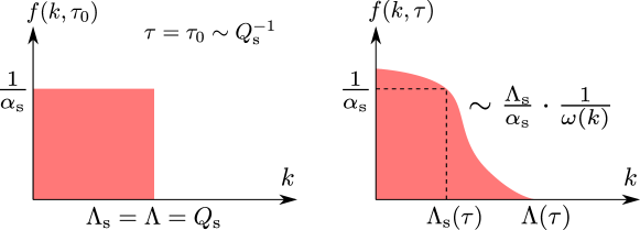
Figure 12: Schematic picture of the real-time evolution of the distribution function from the CGC initial condition (left) to late time profile (right).

An interesting question is to determine the parametric dependence of $\Lambda_{\rm s}(\tau)$ and $\Lambda(\tau)$. According to the arguments in [50] they should parametrically depend on $\tau/\tau_{0}$ as

$$\Lambda_{\rm s}(\tau)\sim Q_{\rm s}\biggl{(}\frac{\tau}{\tau_{0}}\biggr{)}^{-3/7}\;,\qquad\Lambda(\tau)\sim Q_{\rm s}\biggl{(}\frac{\tau}{\tau_{0}}\biggr{)}^{1/7}\;.$$ (87)

The derivation of the above results is as follows. The total energy $\sim\Lambda_{\rm s}\Lambda^{3}$ should be conserved, for which the energy is dominated by a contribution from the window in (86) with the UV cutoff by $\Lambda$. (The contribution from $|\boldsymbol{k}|<\Lambda_{\rm s}$ is suppressed by $(\Lambda_{\rm s}/\Lambda)^{2}$.) Obviously (87) satisfies this condition. Another condition comes from the typical time scale $\tau_{\rm scat}$ of the collision, which can be estimated from the scattering amplitude squared. For example of the $2\leftrightarrow 2$ scattering, $\tau_{\rm scat}^{-1}\sim\alpha_{\rm s}^{2}(\Lambda_{\rm s}/\alpha_{\rm s})^{2}\Lambda^{-1}\sim\Lambda_{\rm s}^{2}\Lambda^{-1}$ with $\Lambda_{\rm s}/\alpha_{\rm s}$ appearing from the distribution. With the concrete form of the kinetic equation, it is concluded [50] that $\tau\sim\tau_{\rm scat}\sim\Lambda_{\rm s}^{-2}\Lambda$, from which (87) follows.

If the thermalization occurs, there should be a clear scale separation between the hard and the soft components by the difference in terms of the strong coupling constant, i.e., the thermalization condition could be chosen as $\Lambda\sim T$ and $\Lambda_{\rm s}\sim\alpha_{\rm s}T$, which implies together with (87) that the thermalization time is estimated as

$$Q_{\rm s}\tau_{\rm th}\sim\alpha_{\rm s}^{-7/4}\;,\qquad T/Q_{\rm s}\sim\alpha_{\rm s}^{-1/4}\;,$$ (88)

which makes a sharp contrast to (15) in the bottom-up thermalization scenario.

The above-mentioned arguments lead us to an interesting speculation. The initially adopted distribution of gluons (left of figure 12) gives the number of gluons as $n_{0}=n_{\rm g}(\tau_{0})\sim Q_{\rm s}^{3}/\alpha_{\rm s}$, which evolves as $n_{\rm g}(\tau)\sim\Lambda^{2}\Lambda_{\rm s}/\alpha_{\rm s}$ in later time (right of figure 12) and at $\tau=\tau_{\rm th}$ the thermal gluon number is naturally $n_{\rm g}(\tau_{\rm th})\sim T^{3}\sim\alpha_{\rm s}^{-3/4}Q_{\rm s}^{3}$. If the elastic scatterings are dominant over the inelastic ones (which is the case for $f\gg 1$), the gluon number can be regarded as a conserved quantity. Then, the discrepancy between $n_{0}$ and $n_{\rm g}(\tau_{\rm th})$ should be sent to a condensate at zero mode, that is, the gluonic BEC should develop so that the condensed gluon number,

$$n_{\rm c}=n_{0}-n_{\rm g}(\tau_{\rm th})\sim\bigl{(}1-\alpha_{\rm s}^{1/4}\bigr{)}\frac{Q_{\rm s}^{3}}{\alpha_{\rm s}}\;,$$ (89)

can compensate for the mismatch. For a realistic situation with $\alpha_{\rm s}\sim 0.3$ for instance, (89) means that about $26\%$ of initially saturated gluons should fall into a BEC when thermalization is achieved. Of course, this estimate is based on quite optimistic simplification.

5.2 Dynamical Evolution of the Spectral Cascade

Let us now consider the evolution of the whole spectral shape. It is a common phenomenon that a power-law spectrum appears as a steady solution out of equilibrium. We can find the power index from the kinetic equation arguments.

5.2.1 Energy cascade vs. particle cascade

To consider the dynamical evolution of the power-law spectrum in QCD, it would be very helpful to gain more general understanding for the spectrum associated with the wave turbulence. Wave turbulence is a phenomenon that occurs in random non-linear waves such as gravity-capillary waves and should be clearly distinguished from the hydrodynamic turbulence.

The theoretical setup is as follows; the system has constant energy pumping at small $k_{-}$ and energy damping at larger $k_{+}$ and we can use the kinetic equation in an interval, $k_{-}\ll k\ll k_{+}$ to describe the wave turbulence to find an index $\nu$ of the Kolmogorov-Zakharov (KZ) spectrum that characterizes the distribution function as

$$f(\boldsymbol{k})\sim\frac{1}{k^{\nu}}\;.$$ (90)

For a given collision kernel of, for example, $2\leftrightarrow 2$ scattering, we can identify the value of $\nu$, and there may sometimes be multiple solutions; one corresponds to the energy cascade and the other corresponds to the particle cascade.

It is easier to find $\nu$ using the continuity equation rather than solving the Boltzmann equation. Let us consider a scattering process involving $p$ particles (waves), and suppose the following scaling properties for the energy dispersion relation and the scattering amplitude as

$$\omega(\mu\boldsymbol{k})=\mu^{\alpha}\omega(\boldsymbol{k})\;,\qquad\mathcal{M}(\mu\boldsymbol{k}_{1},\mu\boldsymbol{k}_{2},\dots)=\mu^{\beta}\mathcal{M}(\boldsymbol{k}_{1},\boldsymbol{k}_{2},\dots)\;.$$ (91)

We first consider the energy cascade, as a result of which the energy spectrum becomes time independent. In terms of the distribution function the one-dimensional energy spectrum is written down as

$$E_{k}(t)=\int\rmd\Omega\,k^{d-1}\omega(\boldsymbol{k})f(\boldsymbol{k},t)\;.$$ (92)

Here, $d$ represents the number of spatial dimensions. The energy conservation is expressed by the energy continuity equation:

$$\frac{\partial E_{k}}{\partial t}+\frac{\partial\varepsilon_{k}}{\partial k}=0\;,$$ (93)

where the energy flow flux is given by

$$\varepsilon_{k}=\int_{k_{+}}^{k}\rmd q\int\rmd\Omega\,q^{d-1}\omega(\boldsymbol{q})\,\biggl{(}\frac{\partial f}{\partial t}\biggr{)}_{\rm coll}\sim k^{(p-1)d-p\alpha+2\beta-\nu(p-1)}\;.$$ (94)

When the system reaches a steady state in terms of the energy, $\partial E_{k}/\partial t=0$ is realized, and then $\varepsilon_{k}$ must be independent of $k$. From this condition of $\varepsilon_{k}\sim k^{0}$ (not the zeroth component but the zeroth power of $k$), we can get to the KZ spectrum index from the energy cascade:

$$\nu_{\rm E}=d+\frac{2\beta-p\alpha}{p-1}\;.$$ (95)

For $2\leftrightarrow 2$ scattering in a (3+1)-dimensional massless scalar theory, $d=3$, $\alpha=1$, and $\beta=0$ and thus we have $\nu_{\rm E}=5/3$. We note that the above mentioned derivation of the index for the KZ spectrum is quite analogous to the famous Kolmogorov spectrum $E_{k}\sim k^{-5/3}$ for hydrodynamic turbulence for which an energy flow flux is assumed to be $k$ independent. Differently from the Kolmogorov spectrum that is fixed by the dimensional analysis, $\nu_{\rm E}$ is sensitive to the structure of microscopic interactions as seen in (95). For example, the capillary waves on deep water has $\nu_{\rm E}=17/4$ (Zakharov-Filonenko spectrum), the acoustic turbulence $\nu_{\rm E}=9/2$ (Zakharov-Sagdeev spectrum), etc. Another branch of the solution belongs to the particle cascade. In this case we should consider the particle number continuity equation:

$$\frac{\partial N_{k}}{\partial t}+\frac{\partial\mu_{k}}{\partial k}=0\;,$$ (96)

where $N_{k}$ is the one-dimensional particle number and $\mu_{k}$ is the particle flow flux, which are defined in the same was as the energy cascade with $\omega(\boldsymbol{k})$ removed from (93) and (94), that after all leads to

$$\nu_{\rm N}=d+\frac{2\beta-(p+1)\alpha}{p-1}\;.$$ (97)

Hence, the particle cascade results in the KZ spectrum with $f\sim k^{-4/3}$ for $2\leftrightarrow 2$ scattering in a massless theory, while it was $f\sim k^{-5/3}$ from the energy cascade.

Generally speaking, the particle cascade occurs in a direction toward smaller $k$ and the energy cascade toward larger $k$. Let us recall that we consider the spectral cascade from $k_{-}$ to $k_{+}$ (where $k_{-}\ll k_{+}$) and introduce the one-particle energy $\omega_{\pm}$ (where $\omega_{-}\ll\omega_{+}$) and the particle flow $\mu_{\pm}$ at $k=k_{\pm}$. Then, the total quantities are $\mu=\mu_{+}+\mu_{-}$ and $\varepsilon=\omega_{+}\mu_{+}+\omega_{-}\mu_{-}$, which leads to

$$\mu\simeq\mu_{-}\;,\qquad\varepsilon\simeq\omega_{+}\mu_{+}\;.$$ (98)

This analysis with (98) implies that the dynamical evolution of the spectrum generally consists of the direct energy cascade (from smaller $k$ to $k_{+}$) and the inverse particle cascade (from larger $k$ to $k_{-}$).

5.2.2 Scenario with non-thermal fixed-point

As explained in section 5.1 it is likely that a certain amount of particles fall into the zero mode if the initial state is overpopulated and the particle number is approximately conserved. Once this situation happens the expected spectrum should be changed because a condensate allows for $1\leftrightarrow 2$ scattering. This means that we should plug $p=3$ (keeping $\beta=0$ because a scalar condensate does not scale with the momentum) into (95) and (97) to find,

$$\nu_{\rm E}=\frac{3}{2}\;,\qquad\nu_{\rm N}=1\;.$$ (99)

In this case, there is another possibility, which is referred to as the non-thermal fixed point [73]. We note that the indices identified with the Boltzmann equations should be valid in the perturbative regime only and the collision terms must involve infinite Feynman diagrams once the interaction goes beyond the perturbatively manageable range. Such non-perturbative treatments are mandatory once the coupling constant ($\lambda$ in a scalar theory) and/or the distribution function $f$ become large. Actually, if $f\gtrsim 1/\lambda$ in a scalar theory or $f\gtrsim 1/\alpha_{\rm s}$ in the saturated regime of QCD, there should be more contributions from terms with more $f$’s and a simple counting in (94) breaks down.

Then, we should switch the theoretical tool from the perturbative Boltzmann equation to the non-perturbative Dyson-Schwinger (or Kadanoff-Baym) equation to look for the scaling solution. This question was addressed in [73] within the framework of the 2PI large-$N$ expansion of $O(N)$ scalar theory with a condensation field. The analytical solution is either $\nu=4$ or $5$ and the numerical simulation favors $\nu=4$, and it has been concluded in [73] that

$$\nu_{\tiny\mbox{non-thermal}}=4\;.$$ (100)

A similar analysis by means of the Dyson-Schwinger equation has been performed in a pure Yang-Mills theory in [111], and it was found that $\nu=2$ and $5$ and even intermediate values might be possible.

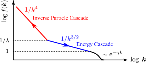
Figure 13: Speculated distribution spectrum with a condensate at zero mode (without expansion). Figure is adapted from [112].

Later, the scenario has been summarized as a diagram in figure 13 according to Berges, and this has been confirmed by the classical statistical simulation in [112]. When $f(\boldsymbol{k})\lesssim 1$ quantum fluctuations dissipate high momentum modes into heat and the tail behaves as $f\sim\rme^{-\gamma k}$. In the regime where $1\ll f(\boldsymbol{k})\ll 1/\lambda$, the kinetic theory works and, as we already saw in the previous subsection, the direct energy cascade is dominant for the flow to larger $k$, leading to $f\sim 1/k^{3/2}$. For small momenta the inverse particle cascade is attributed to the BEC formation, but in this regime with $f(\boldsymbol{k})\gg 1/\lambda$ the perturbative kinetic equation is no longer useful. Thus, instead of $\nu=1$, the index of the non-thermal fixed point, $\nu=4$, should be the expected answer.

It is of course the most interesting question what would be the answer for the situation relevant for the heavy-ion collision physics. It is still unclear whether a gluonic BEC could be formed in the classical statistical simulation [113] (see also [114] for analogous Higgs models). It is even more non-trivial how the scenario should be modified by the expansion effect. So far, all the discussions were focused on the massless case only, and the mass effect was recently analyzed in [115] in the case without expansion, and no qualitative difference was found between the massless and the massive cases.

6 Further Topics

There are many important topics that could not be covered by this review due to limitation of the author’s ability. As a final remark, here, we would not try to name all of such uncovered topics, but we shall pay our attention to a particular problem, that is, the quark production in the very early stage in the heavy-ion collision. The pictorial view in figure 2 leads us to the theoretical formulation of the particle production according to the well-known Schwinger mechanism. In general, non-perturbatively, the production amplitude is given by a Bogoliubov coefficient associated with the basis transformation that connects quark states in the asymptotic past and in the asymptotic future. The Bogoliubov coefficient encompasses all the perturbative processes, which can be easily confirmed by perturbative expansion of the coefficient in terms of the coupling constant.

The numerical simulation on top of the glasma configurations already exists [116] and it claims that most of quarks are produced in a time scale $\lesssim Q_{\rm s}^{-1}$. In fact, in the limit of infinitely thin nuclear sheets at high energies, the quark production dominantly occurs at the light-cone singularity where the color sources propagate, and thus, even at $\tau=0^{+}$, more than a half of total quarks are produced instantly. In the context of the isotropization that we put our emphasis on in this review, the produced quarks would hardly change the qualitative properties such as the isotropization and the universal scaling exponents even though the backreaction from the quark to the gauge sectors is taken into account [117]. Nevertheless, the problem of quark production would spice our problem with a new physics opportunity, i.e., the chirality.

The reason why the chirality is such a special character of matter is that it couples with the quantum anomaly and the QCD $\theta$-vacuum structure. Fortunately, the heavy-ion collision is an ideal environment for such a study to explore anomaly-induced novel phenomena; we have the production of (almost) chiral quarks, and we also have an experimental probe, that is, a strong magnetic field. The coupling between the chirality and the magnetic field would generate topological currents from the chiral magnetic effect, the chiral separation effect, the chiral vortical effect, etc. A full explanation of those chiral topological effects requires another 30 pages review, and we would not go into further technical details on this. Interested readers can consult a recent status summary [118].

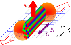
Figure 14: Particle production on top of color flux tubes in the presence of magnetic field. Figure taken from [119].

Most importantly, the color flux tube structure in the glasma initial condition accommodates a bunch of domains with parallel color electric and magnetic fields. Because the electric field is a vector and the magnetic field is an axial vector, the inner product of them is parity-odd (and charge-parity-odd too). Thus, the initial condition in the heavy-ion collision has large topological fluctuations (see [120] for a recent simulation to quantify this effect). Naturally, as sketched in figure 14, the momentum distribution $f(\boldsymbol{k})$ of produced quarks must exhibit some anisotropy under the influence of external magnetic field. Indeed, such skewed $f(\boldsymbol{k})$ was observed in an idealized simulation with homogeneous Abelian fields [121]. Efforts along these directions should be appreciated, for the lifetime of the magnetic field is known to be as short as comparable to $\sim Q_{\rm s}^{-1}$. Anomalous hydrodynamics and chiral kinetic theory should be enumerated as outstanding theoretical developments inspired by the chiral topological effects. However, they both need an initial condition for any practical application, and the initial condition should be given at the glasma time scale.

As stated in the very beginning of this review, early thermalization is the last and greatest unsolved problem in the heavy-ion collision. We might as well say that chiral topological effect is the novel and hottest unresolved challenge in the heavy-ion collision. A marriage of these investigations would produce fruitful offsprings.

K. F. thanks Jürgen Berges, Jean-Paul Blaizot, Francois Gelis, Alexi Kurkela, Jinfeng Liao, Larry McLerran, Jan Pawlowski, Sören Schlichting, Mike Strickland, Raju Venugopalan for extremely useful conversations, through which he learnt a lot. This work was supported by Japanese MEXT grant (No. 15H03652 and 15K13479).

References

References

- [1] G. Baym, “RHIC: From dreams to beams in two decades,” Nucl. Phys. A698 (2002) XXIII–XXXII, arXiv:hep-ph/0104138 [hep-ph].
- [2] G. Baym, “Thermal equilibration in ultrarelativistic heavy ion collisions,” Phys. Lett. B138 (1984) 18–22.
- [3] Y. V. Kovchegov, “Can thermalization in heavy ion collisions be described by QCD diagrams?,” Nucl. Phys. A762 (2005) 298–325, arXiv:hep-ph/0503038 [hep-ph].
- [4] Y. V. Kovchegov, “NonAbelian Weizsacker-Williams field and a two-dimensional effective color charge density for a very large nucleus,” Phys. Rev. D54 (1996) 5463–5469, arXiv:hep-ph/9605446 [hep-ph].
- [5] J. Berges, S. Borsanyi, and C. Wetterich, “Prethermalization,” Phys. Rev. Lett. 93 (2004) 142002, arXiv:hep-ph/0403234 [hep-ph].
- [6] M. Nopoush, R. Ryblewski, and M. Strickland, “Anisotropic hydrodynamics for conformal Gubser flow,” Phys. Rev. D91 (2015) no. 4, 045007, arXiv:1410.6790 [nucl-th].
- [7] T. Hirano, P. Huovinen, K. Murase, and Y. Nara, “Integrated dynamical approach to relativistic heavy ion collisions,” Prog. Part. Nucl. Phys. 70 (2013) 108–158, arXiv:1204.5814 [nucl-th].
- [8] A. M. Stasto, K. J. Golec-Biernat, and J. Kwiecinski, “Geometric scaling for the total cross-section in the low x region,” Phys. Rev. Lett. 86 (2001) 596–599, arXiv:hep-ph/0007192 [hep-ph].
- [9] D. Kharzeev, E. Levin, and M. Nardi, “Color glass condensate at the LHC: Hadron multiplicities in pp, pA and AA collisions,” Nucl. Phys. A747 (2005) 609–629, arXiv:hep-ph/0408050 [hep-ph].
- [10] E. Iancu, K. Itakura, and L. McLerran, “Geometric scaling above the saturation scale,” Nucl. Phys. A708 (2002) 327–352, arXiv:hep-ph/0203137 [hep-ph].
- [11] J. Jalilian-Marian, A. Kovner, A. Leonidov, and H. Weigert, “The BFKL equation from the Wilson renormalization group,” Nucl. Phys. B504 (1997) 415–431, arXiv:hep-ph/9701284 [hep-ph].
- [12] E. Iancu, A. Leonidov, and L. D. McLerran, “Nonlinear gluon evolution in the color glass condensate. 1.,” Nucl. Phys. A692 (2001) 583–645, arXiv:hep-ph/0011241 [hep-ph].
- [13] E. Ferreiro, E. Iancu, A. Leonidov, and L. McLerran, “Nonlinear gluon evolution in the color glass condensate. 2.,” Nucl. Phys. A703 (2002) 489–538, arXiv:hep-ph/0109115 [hep-ph].
- [14] Y. Hatta, E. Iancu, L. McLerran, A. Stasto, and D. N. Triantafyllopoulos, “Effective Hamiltonian for QCD evolution at high energy,” Nucl. Phys. A764 (2006) 423–459, arXiv:hep-ph/0504182 [hep-ph].
- [15] K. Fukushima, “Deriving the Jalilian-Marian-Iancu-McLerran-Weigert-Leonidov-Kovner equation with classical and quantum source terms,” Nucl. Phys. A775 (2006) 69–88, arXiv:hep-ph/0603044 [hep-ph].
- [16] F. Gelis, “Color glass condensate and glasma,” Int. J. Mod. Phys. A28 (2013) 1330001, arXiv:1211.3327 [hep-ph].
- [17] L. D. McLerran and R. Venugopalan, “Computing quark and gluon distribution functions for very large nuclei,” Phys. Rev. D49 (1994) 2233–2241, arXiv:hep-ph/9309289 [hep-ph].
- [18] E. Iancu, K. Itakura, and L. McLerran, “A Gaussian effective theory for gluon saturation,” Nucl. Phys. A724 (2003) 181–222, arXiv:hep-ph/0212123 [hep-ph].
- [19] K. Fukushima and Y. Hidaka, “Light projectile scattering off the color glass condensate,” JHEP 06 (2007) 040, arXiv:0704.2806 [hep-ph].
- [20] A. Kovner, L. D. McLerran, and H. Weigert, “Gluon production from nonAbelian Weizsacker-Williams fields in nucleus-nucleus collisions,” Phys. Rev. D52 (1995) 6231–6237, arXiv:hep-ph/9502289 [hep-ph].
- [21] K. Fukushima, “Evolving Glasma and Kolmogorov spectrum,” Acta Phys. Polon. B42 (2011) 2697–2715, arXiv:1111.1025 [hep-ph].
- [22] T. Lappi and L. McLerran, “Some features of the glasma,” Nucl. Phys. A772 (2006) 200–212, arXiv:hep-ph/0602189 [hep-ph].
- [23] A. Dumitru, F. Gelis, L. McLerran, and R. Venugopalan, “Glasma flux tubes and the near side ridge phenomenon at RHIC,” Nucl. Phys. A810 (2008) 91–108, arXiv:0804.3858 [hep-ph].
- [24] D. Kharzeev, A. Krasnitz, and R. Venugopalan, “Anomalous chirality fluctuations in the initial stage of heavy ion collisions and parity odd bubbles,” Phys. Lett. B545 (2002) 298–306, arXiv:hep-ph/0109253 [hep-ph].
- [25] A. Dumitru, H. Fujii, and Y. Nara, “Magnetic screening in high-energy heavy-ion collisions,” Phys. Rev. D88 (2013) 031503, arXiv:1305.2780 [hep-ph].
- [26] K. Fukushima and F. Gelis, “The evolving Glasma,” Nucl. Phys. A874 (2012) 108–129, arXiv:1106.1396 [hep-ph].
- [27] A. Krasnitz and R. Venugopalan, “Nonperturbative computation of gluon minijet production in nuclear collisions at very high-energies,” Nucl. Phys. B557 (1999) 237, arXiv:hep-ph/9809433 [hep-ph].
- [28] T. Lappi, “Energy density of the glasma,” Phys. Lett. B643 (2006) 11–16, arXiv:hep-ph/0606207 [hep-ph].
- [29] K. Fukushima, “Initial fields and instability in the classical model of the heavy-ion collision,” Phys. Rev. C76 (2007) 021902, arXiv:0711.2634 [hep-ph]. [Erratum: Phys. Rev.C77,029901(2007)].
- [30] R. J. Fries, J. I. Kapusta, and Y. Li, “Near-fields and initial energy density in the color glass condensate model,” arXiv:nucl-th/0604054 [nucl-th].
- [31] H. Fujii, K. Fukushima, and Y. Hidaka, “Initial energy density and gluon distribution from the Glasma in heavy-ion collisions,” Phys. Rev. C79 (2009) 024909, arXiv:0811.0437 [hep-ph].
- [32] R. Baier, A. H. Mueller, D. Schiff, and D. T. Son, “‘Bottom up’ thermalization in heavy ion collisions,” Phys. Lett. B502 (2001) 51–58, arXiv:hep-ph/0009237 [hep-ph].
- [33] S. Mrowczynski, “Stream instabilities of the quark-gluon plasma,” Phys. Lett. B214 (1988) 587. [Erratum: Phys. Lett.B656,273(2007)].
- [34] S. Mrowczynski, “Plasma instability at the initial stage of ultrarelativistic heavy ion collisions,” Phys. Lett. B314 (1993) 118–121.
- [35] P. B. Arnold, J. Lenaghan, and G. D. Moore, “QCD plasma instabilities and bottom up thermalization,” JHEP 08 (2003) 002, arXiv:hep-ph/0307325 [hep-ph].
- [36] H. Fujii and K. Itakura, “Expanding color flux tubes and instabilities,” Nucl. Phys. A809 (2008) 88–109, arXiv:0803.0410 [hep-ph].
- [37] A. Rebhan, P. Romatschke, and M. Strickland, “Hard-loop dynamics of non-Abelian plasma instabilities,” Phys. Rev. Lett. 94 (2005) 102303, arXiv:hep-ph/0412016 [hep-ph].
- [38] A. Dumitru and Y. Nara, “QCD plasma instabilities and isotropization,” Phys. Lett. B621 (2005) 89–95, arXiv:hep-ph/0503121 [hep-ph].
- [39] A. Dumitru, Y. Nara, and M. Strickland, “Ultraviolet avalanche in anisotropic non-Abelian plasmas,” Phys. Rev. D75 (2007) 025016, arXiv:hep-ph/0604149 [hep-ph].
- [40] P. Romatschke and R. Venugopalan, “Collective non-Abelian instabilities in a melting color glass condensate,” Phys. Rev. Lett. 96 (2006) 062302, arXiv:hep-ph/0510121 [hep-ph].
- [41] P. Romatschke and R. Venugopalan, “The Unstable glasma,” Phys. Rev. D74 (2006) 045011, arXiv:hep-ph/0605045 [hep-ph].
- [42] K. Fukushima, “Turbulent pattern formation and diffusion in the early-time dynamics in relativistic heavy-ion collisions,” Phys. Rev. C89 (2014) no. 2, 024907, arXiv:1307.1046 [hep-ph].
- [43] T. S. Biro, C. Gong, B. Muller, and A. Trayanov, “Hamiltonian dynamics of Yang-Mills fields on a lattice,” Int. J. Mod. Phys. C5 (1994) 113–149, arXiv:nucl-th/9306002 [nucl-th].
- [44] U. W. Heinz, C. R. Hu, S. Leupold, S. G. Matinyan, and B. Muller, “Thermalization and Lyapunov exponents in the Yang-Mills Higgs theory,” Phys. Rev. D55 (1997) 2464–2476, arXiv:hep-th/9608181 [hep-th].
- [45] T. Kunihiro, B. Muller, A. Ohnishi, A. Schafer, T. T. Takahashi, and A. Yamamoto, “Chaotic behavior in classical Yang-Mills dynamics,” Phys. Rev. D82 (2010) 114015, arXiv:1008.1156 [hep-ph].
- [46] H. Iida, T. Kunihiro, B. Mueller, A. Ohnishi, A. Schaefer, and T. T. Takahashi, “Entropy production in classical Yang-Mills theory from Glasma initial conditions,” Phys. Rev. D88 (2013) 094006, arXiv:1304.1807 [hep-ph].
- [47] P. B. Arnold, G. D. Moore, and L. G. Yaffe, “Effective kinetic theory for high temperature gauge theories,” JHEP 01 (2003) 030, arXiv:hep-ph/0209353 [hep-ph].
- [48] A. Kurkela and Y. Zhu, “Isotropization and hydrodynamization in weakly coupled heavy-ion collisions,” Phys. Rev. Lett. 115 (2015) no. 18, 182301, arXiv:1506.06647 [hep-ph].
- [49] J.-P. Blaizot, J. Liao, and L. McLerran, “Gluon transport equation in the small angle approximation and the onset of Bose-Einstein condensation,” Nucl. Phys. A920 (2013) 58–77, arXiv:1305.2119 [hep-ph].
- [50] J.-P. Blaizot, F. Gelis, J.-F. Liao, L. McLerran, and R. Venugopalan, “Bose–Einstein condensation and thermalization of the Quark Gluon Plasma,” Nucl. Phys. A873 (2012) 68–80, arXiv:1107.5296 [hep-ph].
- [51] J.-P. Blaizot, J. Liao, and Y. Mehtar-Tani, “The subtle interplay of elastic and inelastic collisions in the thermalization of the quark-gluon plasma,” in 25th International Conference on Ultra-Relativistic Nucleus-Nucleus Collisions (Quark Matter 2015) Kobe, Japan, September 27-October 3, 2015. 2016. arXiv:1601.00308 [nucl-th].
- [52] K. Fukushima, F. Gelis, and L. McLerran, “Initial singularity of the little bang,” Nucl. Phys. A786 (2007) 107–130, arXiv:hep-ph/0610416 [hep-ph].
- [53] T. Kunihiro, B. Muller, A. Ohnishi, and A. Schafer, “Towards a theory of entropy production in the little and big bang,” Prog. Theor. Phys. 121 (2009) 555–575, arXiv:0809.4831 [hep-ph].
- [54] R. Micha and I. I. Tkachev, “Relativistic turbulence: A Long way from preheating to equilibrium,” Phys. Rev. Lett. 90 (2003) 121301, arXiv:hep-ph/0210202 [hep-ph].
- [55] R. Micha and I. I. Tkachev, “Turbulent thermalization,” Phys. Rev. D70 (2004) 043538, arXiv:hep-ph/0403101 [hep-ph].
- [56] G. Aarts and J. Berges, “Classical aspects of quantum fields far from equilibrium,” Phys. Rev. Lett. 88 (2002) 041603, arXiv:hep-ph/0107129 [hep-ph].
- [57] J. Berges, S. Scheffler, and D. Sexty, “Bottom-up isotropization in classical-statistical lattice gauge theory,” Phys. Rev. D77 (2008) 034504, arXiv:0712.3514 [hep-ph].
- [58] J. Berges, “Nonequilibrium quantum fields: From cold atoms to cosmology,” arXiv:1503.02907 [hep-ph].
- [59] K. Dusling, F. Gelis, and R. Venugopalan, “The initial spectrum of fluctuations in the little bang,” Nucl. Phys. A872 (2011) 161–195, arXiv:1106.3927 [nucl-th].
- [60] K. Dusling, T. Epelbaum, F. Gelis, and R. Venugopalan, “Instability induced pressure isotropization in a longitudinally expanding system,” Phys. Rev. D86 (2012) 085040, arXiv:1206.3336 [hep-ph].
- [61] T. Epelbaum and F. Gelis, “Fluctuations of the initial color fields in high energy heavy ion collisions,” Phys. Rev. D88 (2013) 085015, arXiv:1307.1765 [hep-ph].
- [62] K. Fukushima, “Spectral representation of the particle production out of equilibrium - Schwinger mechanism in pulsed electric fields,” New J. Phys. 16 (2014) 073031, arXiv:1402.3002 [hep-ph].
- [63] T. Epelbaum and F. Gelis, “Pressure isotropization in high energy heavy ion collisions,” Phys. Rev. Lett. 111 (2013) 232301, arXiv:1307.2214 [hep-ph].
- [64] T. Epelbaum, F. Gelis, and B. Wu, “Nonrenormalizability of the classical statistical approximation,” Phys. Rev. D90 (2014) no. 6, 065029, arXiv:1402.0115 [hep-ph].
- [65] A. H. Mueller and D. T. Son, “On the Equivalence between the Boltzmann equation and classical field theory at large occupation numbers,” Phys. Lett. B582 (2004) 279–287, arXiv:hep-ph/0212198 [hep-ph].
- [66] S. Jeon, “The Boltzmann equation in classical and quantum field theory,” Phys. Rev. C72 (2005) 014907, arXiv:hep-ph/0412121 [hep-ph].
- [67] T. Epelbaum, F. Gelis, N. Tanji, and B. Wu, “Properties of the Boltzmann equation in the classical approximation,” Phys. Rev. D90 (2014) no. 12, 125032, arXiv:1409.0701 [hep-ph].
- [68] C. Connaughton, C. Josserand, A. Picozzi, Y. Pomeau, and S. Rica, “Condensation of classical nonlinear waves,” Phys. Rev. Lett. 95 (2005) 263901.
- [69] T. Epelbaum, F. Gelis, S. Jeon, G. Moore, and B. Wu, “Kinetic theory of a longitudinally expanding system of scalar particles,” JHEP 09 (2015) 117, arXiv:1506.05580 [hep-ph].
- [70] T. Gasenzer and J. M. Pawlowski, “Towards far-from-equilibrium quantum field dynamics: A functional renormalisation-group approach,” Phys. Lett. B670 (2008) 135–140.
- [71] J. M. Cornwall, R. Jackiw, and E. Tomboulis, “Effective action for composite operators,” Phys. Rev. D10 (1974) 2428–2445.
- [72] G. Aarts, D. Ahrensmeier, R. Baier, J. Berges, and J. Serreau, “Far from equilibrium dynamics with broken symmetries from the 2PI– expansion,” Phys. Rev. D66 (2002) 045008, arXiv:hep-ph/0201308 [hep-ph].
- [73] J. Berges, A. Rothkopf, and J. Schmidt, “Non-thermal fixed points: Effective weak-coupling for strongly correlated systems far from equilibrium,” Phys. Rev. Lett. 101 (2008) 041603, arXiv:0803.0131 [hep-ph].
- [74] J. Berges and M. M. Muller, “Nonequilibrium quantum fields with large fluctuations,” in 285th Heraeus Seminar: Interdisciplinary Workshop on Progress in Nonequilibrium Greens Functions (Kadanoff-Baym Equations II) Dresden, Gremany, August 19-23, 2002. 2002. arXiv:hep-ph/0209026 [hep-ph].
- [75] W. Cassing, “From Kadanoff-Baym dynamics to off-shell parton transport,” Eur. Phys. J. ST 168 (2009) 3–87, arXiv:0808.0715 [nucl-th].
- [76] Y. Hatta and A. Nishiyama, “Towards thermalization in heavy-ion collisions: CGC meets the 2PI formalism,” Nucl. Phys. A873 (2012) 47–67, arXiv:1108.0818 [hep-ph].
- [77] E. Nelson, “Derivation of the Schrodinger equation from Newtonian mechanics,” Phys. Rev. 150 (1966) 1079–1085.
- [78] P. H. Damgaard and H. Huffel, “Stochastic quantization,” Phys. Rept. 152 (1987) 227.
- [79] J. Berges and I. O. Stamatescu, “Simulating nonequilibrium quantum fields with stochastic quantization techniques,” Phys. Rev. Lett. 95 (2005) 202003, arXiv:hep-lat/0508030 [hep-lat].
- [80] J. Berges and D. Sexty, “Real-time gauge theory simulations from stochastic quantization with optimized updating,” Nucl. Phys. B799 (2008) 306–329, arXiv:0708.0779 [hep-lat].
- [81] R. Anzaki, K. Fukushima, Y. Hidaka, and T. Oka, “Restricted phase-space approximation in real-time stochastic quantization,” Annals Phys. 353 (2015) 107–128, arXiv:1405.3154 [hep-ph].
- [82] G. Aarts, L. Bongiovanni, E. Seiler, and D. Sexty, “Some remarks on Lefschetz thimbles and complex Langevin dynamics,” JHEP 10 (2014) 159, arXiv:1407.2090 [hep-lat].
- [83] K. Fukushima and Y. Tanizaki, “Hamilton dynamics for Lefschetz-thimble integration akin to the complex Langevin method,” arXiv:1507.07351 [hep-th].
- [84] T. Hayata, Y. Hidaka, and Y. Tanizaki, “Complex saddle points and the sign problem in complex Langevin simulation,” arXiv:1511.02437 [hep-lat].
- [85] H. Fujii, S. Kamata, and Y. Kikukawa, “Lefschetz thimble structure in one-dimensional lattice Thirring model at finite density,” JHEP 11 (2015) 078, arXiv:1509.08176 [hep-lat]. [Erratum: JHEP02,036(2016)].
- [86] G. Policastro, D. T. Son, and A. O. Starinets, “The Shear viscosity of strongly coupled N=4 supersymmetric Yang-Mills plasma,” Phys. Rev. Lett. 87 (2001) 081601, arXiv:hep-th/0104066 [hep-th].
- [87] R. A. Janik and R. B. Peschanski, “Asymptotic perfect fluid dynamics as a consequence of Ads/CFT,” Phys. Rev. D73 (2006) 045013, arXiv:hep-th/0512162 [hep-th].
- [88] Y. V. Kovchegov and A. Taliotis, “Early time dynamics in heavy ion collisions from AdS/CFT correspondence,” Phys. Rev. C76 (2007) 014905, arXiv:0705.1234 [hep-ph].
- [89] R. Peschanski, “Introduction to string theory and gauge/gravity duality for students in QCD and QGP phenomenology,” Acta Phys. Polon. B39 (2008) 2479–2510, arXiv:0804.3210 [hep-ph].
- [90] R. A. Janik, “The dynamics of quark-gluon plasma and AdS/CFT,” Lect. Notes Phys. 828 (2011) 147–181, arXiv:1003.3291 [hep-th].
- [91] P. M. Chesler and L. G. Yaffe, “Horizon formation and far-from-equilibrium isotropization in supersymmetric Yang-Mills plasma,” Phys. Rev. Lett. 102 (2009) 211601, arXiv:0812.2053 [hep-th].
- [92] P. M. Chesler and L. G. Yaffe, “Holography and colliding gravitational shock waves in asymptotically AdS5 spacetime,” Phys. Rev. Lett. 106 (2011) 021601, arXiv:1011.3562 [hep-th].
- [93] J. Berges, K. Boguslavski, S. Schlichting, and R. Venugopalan, “Universal attractor in a highly occupied non-Abelian plasma,” Phys. Rev. D89 (2014) no. 11, 114007, arXiv:1311.3005 [hep-ph].
- [94] D. Bodeker, “The Impact of QCD plasma instabilities on bottom-up thermalization,” JHEP 10 (2005) 092, arXiv:hep-ph/0508223 [hep-ph].
- [95] A. Kurkela and G. D. Moore, “Bjorken flow, plasma instabilities, and thermalization,” JHEP 11 (2011) 120, arXiv:1108.4684 [hep-ph].
- [96] J. Berges, K. Boguslavski, S. Schlichting, and R. Venugopalan, “Universality far from equilibrium: From superfluid Bose gases to heavy-ion collisions,” Phys. Rev. Lett. 114 (2015) no. 6, 061601, arXiv:1408.1670 [hep-ph].
- [97] P. C. Hohenberg and B. I. Halperin, “Theory of dynamic critical phenomena,” Rev. Mod. Phys. 49 (1977) 435–479.
- [98] W. Florkowski and R. Ryblewski, “Highly-anisotropic and strongly-dissipative hydrodynamics for early stages of relativistic heavy-ion collisions,” Phys. Rev. C83 (2011) 034907, arXiv:1007.0130 [nucl-th].
- [99] M. Martinez and M. Strickland, “Dissipative dynamics of highly anisotropic systems,” Nucl. Phys. A848 (2010) 183–197, arXiv:1007.0889 [nucl-th].
- [100] A. Muronga, “Causal theories of dissipative relativistic fluid dynamics for nuclear collisions,” Phys. Rev. C69 (2004) 034903, arXiv:nucl-th/0309055 [nucl-th].
- [101] T. Hayata, Y. Hidaka, T. Noumi, and M. Hongo, “Relativistic hydrodynamics from quantum field theory on the basis of the generalized Gibbs ensemble method,” Phys. Rev. D92 (2015) no. 6, 065008, arXiv:1503.04535 [hep-ph].
- [102] A. Muronga, “Second order dissipative fluid dynamics for ultrarelativistic nuclear collisions,” Phys. Rev. Lett. 88 (2002) 062302, arXiv:nucl-th/0104064 [nucl-th]. [Erratum: Phys. Rev. Lett.89,159901(2002)].
- [103] W. Florkowski, “Anisotropic fluid dynamics in the early stage of relativistic heavy-ion collisions,” Phys. Lett. B668 (2008) 32–35, arXiv:0806.2268 [nucl-th].
- [104] W. Florkowski and R. Ryblewski, “Dynamics of anisotropic plasma at the early stages of relativistic heavy-ion collisions,” Acta Phys. Polon. B40 (2009) 2843–2863, arXiv:0901.4653 [nucl-th].
- [105] M. Martinez and M. Strickland, “Constraining relativistic viscous hydrodynamical evolution,” Phys. Rev. C79 (2009) 044903, arXiv:0902.3834 [hep-ph].
- [106] R. Ryblewski and W. Florkowski, “Highly anisotropic hydrodynamics – discussion of the model assumptions and forms of the initial conditions,” Acta Phys. Polon. B42 (2011) 115–138, arXiv:1011.6213 [nucl-th].
- [107] D. Bazow, U. W. Heinz, and M. Strickland, “Second-order (2+1)-dimensional anisotropic hydrodynamics,” Phys. Rev. C90 (2014) no. 5, 054910, arXiv:1311.6720 [nucl-th].
- [108] M. Nopoush, R. Ryblewski, and M. Strickland, “Bulk viscous evolution within anisotropic hydrodynamics,” Phys. Rev. C90 (2014) no. 1, 014908, arXiv:1405.1355 [hep-ph].
- [109] L. Tinti, “(3+1)-dimensional framework for leading-order nonconformal anisotropic hydrodynamics,” Phys. Rev. C92 (2015) no. 1, 014908, arXiv:1411.7268 [nucl-th].
- [110] A. Kurkela and G. D. Moore, “Thermalization in weakly coupled nonabelian plasmas,” JHEP 12 (2011) 044, arXiv:1107.5050 [hep-ph].
- [111] M. E. Carrington and A. Rebhan, “Perturbative and nonperturbative Kolmogorov turbulence in a gluon plasma,” Eur. Phys. J. C71 (2011) 1787, arXiv:1011.0393 [hep-ph].
- [112] J. Berges and D. Sexty, “Bose condensation far from equilibrium,” Phys. Rev. Lett. 108 (2012) 161601, arXiv:1201.0687 [hep-ph].
- [113] J. Berges, S. Schlichting, and D. Sexty, “Over-populated gauge fields on the lattice,” Phys. Rev. D86 (2012) 074006, arXiv:1203.4646 [hep-ph].
- [114] T. Gasenzer, L. McLerran, J. M. Pawlowski, and D. Sexty, “Gauge turbulence, topological defect dynamics, and condensation in Higgs models,” Nucl. Phys. A930 (2014) 163–186, arXiv:1307.5301 [hep-ph].
- [115] J.-P. Blaizot, Y. Jiang, and J. Liao, “Gluon transport equation with effective mass and dynamical onset of Bose-Einstein condensation,” arXiv:1503.07260 [hep-ph].
- [116] F. Gelis, K. Kajantie, and T. Lappi, “Chemical thermalization in relativistic heavy ion collisions,” Phys. Rev. Lett. 96 (2006) 032304, arXiv:hep-ph/0508229 [hep-ph].
- [117] D. Gelfand, F. Hebenstreit, and J. Berges, “Early quark production and approach to chemical equilibrium,” arXiv:1601.03576 [hep-ph].
- [118] J. Liao, “Chiral magnetic effect in heavy ion collisions,” in 25th International Conference on Ultra-Relativistic Nucleus-Nucleus Collisions (Quark Matter 2015) Kobe, Japan, September 27-October 3, 2015. 2016. arXiv:1601.00381 [nucl-th]. https://inspirehep.net/record/1412086/files/arXiv:1601.00381.pdf.
- [119] K. Fukushima, D. E. Kharzeev, and H. J. Warringa, “Real-time dynamics of the Chiral Magnetic Effect,” Phys. Rev. Lett. 104 (2010) 212001, arXiv:1002.2495 [hep-ph].
- [120] M. Mace, S. Schlichting, and R. Venugopalan, “Off-equilibrium sphaleron transitions in the Glasma,” arXiv:1601.07342 [hep-ph].
- [121] K. Fukushima, “Simulating net particle production and chiral magnetic current in a -odd domain,” Phys. Rev. D92 (2015) no. 5, 054009, arXiv:1501.01940 [hep-ph].