Swarming in viscous fluids: three-dimensional patterns in swimmer- and force-induced flows

Abstract

We derive from first principles a three-dimensional theory of self-propelled particle swarming in a viscous fluid environment. Our model predicts emergent collective behavior that depends critically on fluid opacity, mechanism of self-propulsion, and type of particle-particle interaction. In “clear fluids” swimmers have full knowledge of their surroundings and can adjust their velocities with respect to the lab frame, while in “opaque fluids,” they control their velocities only in relation to the local fluid flow. We also show that “social” interactions that affect only a particle’s propensity to swim towards or away from neighbors induces a flow field that is qualitatively different from the long-ranged flow fields generated by direct “physical” interactions. The latter can be short-ranged but lead to much longer-ranged fluid-mediated hydrodynamic forces, effectively amplifying the range over which particles interact. These different fluid flows conspire to profoundly affect swarm morphology, kinetically stabilizing or destabilizing swarm configurations that would arise in the absence of fluid. Depending upon the overall interaction potential, the mechanism of swimming (e.g., pushers or pullers), and the degree of fluid opaqueness, we discover a number of new collective three-dimensional patterns including flocks with prolate or oblate shapes, recirculating peloton-like structures, and jet-like fluid flows that entrain particles mediating their escape from the center of mill-like structures. Our results reveal how the interplay among general physical elements influence fluid-mediated interactions and the self-organization, mobility, and stability of new three-dimensional swarms and suggest how they might be used to kinetically control their collective behavior.

The collective behavior of self-propelled agents in natural and artificial systems has been extensively studied Spohn (1991); Kaufmann (1993); Vicsek et al. (1995); Toner and Tu (1995); Albano (1996); Flierl et al. (1999); Shimoyama et al. (1996); Edelstein-Keshet et al. (1998); Levine et al. (2000); Ebeling and Schweitzer (2001); Parrish et al. (2002); Grégoire et al. (2003); Chalub et al. (2004); Couzin et al. (2005); Dolak and Schmeiser (2005); Morale et al. (2005); D’Orsogna et al. (2006); Chalub et al. (2006); Chuang et al. (2007a); Bernoff and Topaz (2013); Kaiser and Löwen (2013); You (2013). Many of the lessons learned from experimental and theoretical work conducted on organisms as diverse as bacteria, ants, locusts, and birds Schneirla (1971); Kim and Kaiser (1990); Niwa (1994); Dillon et al. (1995); Romey (1996); Koch and White (1998); Parrish and Edelstein-Keshet (1999); Camazine et al. (2003); Ordemann et al. (2003); Oien (2004); Gómez-Mourelo (2005); Mach and Schweitzer (2006); Topaz et al. (2008); Hein and McKinley (2013) have been successfully applied to engineered robotic systems to help frame decentralized control strategies through ad-hoc algorithms Sugawara and Sano (1997); Bonabeau et al. (1999); Leonard and Fiorelli (2001); Gazi and Passino (2003); Chang et al. (2003); Jadbabaie et al. (2003); Liu et al. (2003); Chuang et al. (2007b). In most mathematical “swarming” models, particles are assumed to be self-driven by internal mechanisms that impart a characteristic speed. A pairwise short-ranged repulsion and a long-ranged decaying attraction are typically employed as the most realistic choices when modeling aggregating particles Levine et al. (2000); Parrish et al. (2002); Couzin et al. (2002). The interplay between self-propulsion, particle interactions, initial conditions, and number of particles is key in determining the large scale patterns that dynamically arise. In two dimensions, rotating mills and translating flocks are often observed, the latter configuration also arising in three dimensions Levine et al. (2000); Ebeling and Schweitzer (2001); D’Orsogna et al. (2006); Chuang et al. (2007a); Strefler et al. (2008); Nguyen et al. (2012). It is possible to classify swarm morphology in terms of interaction strength and length scales, as shown for particles coupled via conserved forces derived from the Morse potential D’Orsogna et al. (2006); Chuang et al. (2007a). Externally applied potentials and noise can be also used to trigger transitions between coherent and disordered structures Vicsek et al. (1995); Strefler et al. (2008); Nguyen et al. (2012).

Although different rules for the characteristic speed have been proposed Levine et al. (2000); Ebeling and Schweitzer (2001); D’Orsogna et al. (2006), most studies so far have focused on self-propelled agents in “vacuum”, ignoring the medium in which nearly all real systems operate. One exception is the literature on swimmers wherein models have been developed for a single or a few organisms that propel themselves in viscous Taylor (1951); Hancock (1953); Blake (1973); Shapere and Wilczek (1989); Galdi (1999); Becker et al. (2003); Baskaran and Marchetti (2008); Spagnolie and Lauga (2012); Wolgemuth (2008); Lauga and Powers (2009); Huber et al. (2011) and non-Newtonian fluids Ross and Corrsin (1974); Chaudhury (1979); Fulford et al. (1998); Lauga (2007); Normand and Lauga (2008); Lauga and Powers (2009); Lauga (2009); Fu et al. (2007, 2009); Zhu et al. (2012). In particular, swarming hydrodynamic theories have been derived wherein swimmer densities with or without fluid flows are described as continuous fields Baskaran and Marchetti (2009); Toner and Tu (1995); Chuang et al. (2007a); Solon et al. (2015). These “two fluid” models however may not always display the rich features observed when particles retain their discreteness, especially in terms of finite-sized swarm morphology, stability and self-organization.

To efficiently study the collective dynamics of self-propelled particles in a fluid medium we derive a microscopic three-dimensional “agent-based” kinetic theory that incorporates hydrodynamic interactions between particles. A possible starting point would be to assume that the fluid medium leads to direct coupling between particle velocities and build this effect into existing models using, for example, the Cucker-Smale velocity matching mechanism. Here, particle $i$ is subject to an additional force due to the presence of particle $j$, given by ${\bf v}_{j}-{\bf v}_{i}$ and modulated by a distance-dependent prefactor $g(|{\bf r}_{i}-{\bf r}_{j}|)$ Cucker and Smale (2007a, b); Shen (2008). Because of its simple mathematical form, Cucker-Smale type interactions have been used extensively to study swarming, with coherent morphologies arising depending on the form of $g(|{\bf r}_{i}-{\bf r}_{j}|)$. Although not explicitly meant to model fluid-mediated couplings, a heuristic Cucker-Smale-type interaction could be constructed by choosing an appropriate form for $g(|{\bf r}_{i}-{\bf r}_{j}|)$ or different powers of $|{\bf v}_{i}-{\bf v}_{j}|$. Whether such an approach would be consistent with more microscopic derivation of fluid-mediated particle-particle interactions is however unclear.

The goal of this paper is to derive from first principles a theory of particle swarming in fluids and to understand the ways viscous flows can arise and affect particle dynamics and collective behavior. In order to incorporate fluid couplings into discrete particle models, one must first identify the physical origin of the interactions between particles. In typical models of swarming Levine et al. (2000); Grégoire et al. (2003); Morale et al. (2005); D’Orsogna et al. (2006); Topaz et al. (2008); Bernoff and Topaz (2013), the propensity of agents to self-propel themselves towards or away from others is modulated by an effective “social” interaction potential. When immersed in low-Reynolds number Newtonian fluids, particle self-propulsion is force-free. Here, the fluid flows arising from swimming or squirming particles can be decomposed in terms of force dipoles or higher order force distributions leading to velocities that decay away from the swimmer as $1/r^{n},n\geq 2$ Nasseri and Phan-Thien (1997); Cortez et al. (2004, 2005); Riedel et al. (2005); Ishikawa et al. (2006); Lauga and Powers (2009). The sign and amplitude of this self-propulsion-induced flow field depend on the specific details of the “stroke” of the swimmer Najafi and Golestanian (2004); Wolgemuth (2008); Baskaran and Marchetti (2009); Huber et al. (2011); Spagnolie and Lauga (2012).

A qualitatively different flow arises if the potential is associated with a true “physical” force, arising from, say, electrostatic molecular, magnetic, or gravitational interactions. These physical interactions between swimmers impart an external body force on each of them, ultimately leading to a flow field that decays as $1/r$ Happel and Brenner (1965); Español et al. (1995); Batchelor (2000). Although the physical forces between particles may be short-ranged, they can be transmitted to the surrounding fluid Oseen (1927); Ladyzhenskaya and Silverman (1963); Finn (1965); Blake (1971); Español et al. (1995); Shu and Chwang (2001), collectively generating a much longer-ranged flow field, and effectively extending the range of interactions. Thus, the resulting $1/r$ Oseen flow field can be even longer ranged than the $1/r^{n}$ flows arising from self-propulsion.

The different origins of fluid flow can be most easily understood by considering a single particle moving under a constant chemical gradient or passively sedimenting under a gravitational potential. A chemoattractant can be represented by a “social” interaction as it only directs a force-free self-propeller towards a particular velocity. A body force resulting from e.g., gravity is a physical force since it ultimately imparts a force on the fluid. In both cases, particle trajectories are identical and can be described by motion under a linear effective potential. However, within a fluid medium, a chemotactic social interaction generates a different flow from that of sedimentation under a physical interaction. As we shall see, the qualitatively different fluid flows arising from social and physical interactions also lead to qualitatively different collective particle behavior. How the details of particle-particle interactions are modeled and interpreted thus becomes a critical element in the development and application of hydrodynamically coupled particle swarming theories.

Finally, we also consider two different types of fluids: “clear” and “opaque.” In a clear fluid, particles can “see” fixed markers and have direct knowledge of their motion in reference to the rest frame. Their absolute velocities can be directly controlled by their internal self-propelling mechanism. Here, the surrounding fluid simply imparts an additional drag force. In the richer and more interesting case of an opaque fluid, particles only have near-field vision and their velocities can be governed only in relation to the surrounding flow. For both social and physical interactions, we systematically derive the effective particle-particle coupling arising from viscous Stokes flows and investigate their effects on coherent three dimensional swarming structures. These hydrodynamic interactions strongly affect collective dynamics and give rise to surprising new patterns such as distorted flocks, pelotons, core-filled mills, and mills that perpetually disband and reform.

Fluid-coupled equations of motion

We consider a system of $N$ identical particles with mass $m=1$. We can write the equations of motion for particle $i$ at position ${\bf r}_{i}(t)$ and lab-frame velocity ${\bf v}_{i}(t)$ as follows

$$\dot{{\bf r}}_{i} = {\bf v}_{i},$$

$$\dot{{\bf v}}_{i} = -\gamma({\bf v}_{i}-{\bf u}({\bf r}_{i}))+{\bf f}_{M}({\bf v}_{i},{\bf u}(r_{i}))+{\bf f}_{i}$$ (1)

where ${\bf u}({\bf r}_{i})$ is the lab-frame fluid velocity generated at position ${\bf r}_{i}$ by the motion of all other particles in the absence of particle $i$. In Eq. 1 the drag force $-\gamma({\bf v}_{i}-{\bf u}({\bf r}_{i}))$ on particle $i$ is proportional to its velocity relative to that of the fluid ${\bf u}({\bf r}_{i})$. Without loss of generality, we assume spherical particles with a small radius $a$ and drag coefficient $\gamma=6\pi\eta a$. The force term ${\bf f}_{\rm M}({\bf v}_{i},{\bf u}({\bf r}_{i}))$ represents the self-propelling motility force on particle $i$, which can depend both on ${\bf v}_{i}$ and ${\bf u}({\bf r}_{i})$. It is usually chosen to have non-trivial zeros that identify characteristic speeds of motion. For the purposes of this paper, we adopt a modified friction form given by

$${\bf f}_{M}({\bf v}_{i},{\bf u}({\bf r}_{i}))=(\alpha-\beta|{\bf v}_{i}-\lambda{\bf u}({\bf r}_{i})|^{2}),$$ (2)

where the parameters $\alpha$ and $\beta$ quantify self acceleration and deceleration, respectively. Eq. 2 with $\lambda=0$ yields the classical Rayleigh-Helmholtz friction that has been extensively used to model self-propulsion in vacuum D’Orsogna et al. (2006); Chuang et al. (2007a); Romanczuk et al. (2012); Nguyen et al. (2012). In this case, the natural characteristic speed arises by setting ${\bf f}_{M}$ to zero and is given by $|{\bf v}_{i}|=\sqrt{\alpha/\beta}$. We introduce the “perception coefficient” $\lambda$ in Eq. 2 to represent how well particles sense their environment once they are immersed in a fluid. The choice $\lambda=0$ represents the case where swimmers can determine their lab frame velocities ${\bf v}_{i}$ as if they were in a vacuum and adjust their speed towards the characteristic velocity $\sqrt{\alpha/\beta}$. Thus $\lambda=0$ indicates a “clear” fluid where any effects on particle movement imparted to particles by the fluid will arise only through drag forces. Conversely, the choice $\lambda=1$ indicates that swimmers have no knowledge of the lab frame and can determine their motion only in relation to the local fluid. As a result, swimmers will regulate their relative velocity ${\bf v}_{i}-{\bf u}({\bf r}_{i})$ and not their lab frame velocity ${\bf v}_{i}$ toward the characteristic speed. This is the “opaque” fluid limit. Other values $0<\lambda<1$ yield intermediate regimes. Note that the Rayleigh-Helmholtz friction is not the only option for modeling swarming self propulsion. An in-depth discussion about the effects of choosing different functional forms for self propulsion can be found in Romanczuk et al. (2012); the difference is particularly profound in the presence of noise. Finally

$${\bf f}_{i}=-\nabla_{i}\sum_{j\neq i}\Phi(|{\bf r}_{i}-{\bf r}_{j}|)$$ (3)

is the particle-particle interaction force on particle $i$, where $\nabla_{i}\equiv\partial/\partial{\bf r}_{i}$ and $\Phi(|{\bf r}_{i}-{\bf r}_{j}|)$ is the direct pairwise interaction potential. While any mathematical form for $\Phi(|({\bf r}_{i}-{\bf r}_{j})|$ can be used, to be consistent and comparative with previous literature, we use the commonly studied Morse potential Levine et al. (2000), given by the superposition of repulsive and attractive components

$$\Phi\left(\left|{\bf r}_{i}-{\bf r}_{j}\right|\right)=C_{r}\mathrm{e}^{-\frac{\left|{\bf r}_{i}-{\bf r}_{j}\right|}{\ell_{r}}}-C_{a}\mathrm{e}^{-\frac{\left|{\bf r}_{i}-{\bf r}_{j}\right|}{\ell_{a}}}.$$ (4)

The coefficients $C_{a}$ and $C_{r}$ in Eq. 4 define the strengths of the attractive and repulsive potentials, respectively and $\ell_{a}$ and $\ell_{r}$ specify their effective lengths of interaction. Using this potential, the fluid-free swarming problem (Eq. 1 with ${\bf u}=0$) has been very well studied especially in one and two dimensions Levine et al. (2000); D’Orsogna et al. (2006); Chuang et al. (2007a); Bernoff and Topaz (2013); Topaz and Bertozzi (2004). Generally, particles are subject to two tendencies: changing their separations to minimize $\Phi$ and adjusting their velocities to match the characteristic speed. Depending on initial conditions, dimensionality, number of particles and/or parameter choices, both tendencies can be simultaneously satisfied, leading, for example, to rigidly translating flocks. If only one is satisfied, mills, rigid disks, or random motion arise Chuang et al. (2007a).

For the fluid-coupled equations of motion what now remains is to specify the source of ${\bf u}$. To model ${\bf u}$ we note that in classical swarming models the potential $\Phi$ is usually a mathematical representation of socially derived interactions. In this scenario, the only actual force exerted by the swimming particles on the fluid is via their self propulsion. In this case, the fluid disturbance ${\bf u}\equiv{\bf u}_{\rm s}$ depends only on the microscopic details of the swimming mechanism and decays as $1/r^{n},n\geq 2$ Nasseri and Phan-Thien (1997); Cortez et al. (2004, 2005); Riedel et al. (2005); Ishikawa et al. (2006); Lauga and Powers (2009). In this paper we assume an effective stroke-averaged self-propulsion whereby the swimmer’s period-averaged strokes are described as a force dipole acting on the fluid leading to

$${\bf u}_{\rm s}({\bf r})=\sum_{j}\frac{Gv_{j}}{R_{j}^{2}}\left[3\left(\hat{{\bf R}}_{j}\cdot\hat{\bf v}_{j}\right)^{2}-1\right]\hat{{\bf R}}_{j},$$ (5)

where ${\bf R}_{j}\equiv({\bf r}-{\bf r}_{j})$, $R_{j}\equiv\left|{\bf R}_{j}\right|$, $\hat{{\bf R}}_{j}\equiv{\bf R}_{j}/R_{j}$, $v_{j}\equiv\left|{\bf v}_{j}\right|$, and $\hat{{\bf v}}_{j}\equiv{\bf v}_{j}/v_{j}$ Baskaran and Marchetti (2009). Here, the social potential $\Phi$ influences ${\bf u}_{\rm s}({\bf r})$ through $v_{j}$ which obeys Eq. 1. The lumped parameter $G$ in Eq. 5 depends on the details of swimmer geometry such as its length and longitudinal mass distribution, and carries units of a length squared. For $G>0$, the orientation of the force dipole is parallel to the swimmer’s velocity, describing a propelling swimmer or a “pusher”; conversely, $G<0$ denotes a contractile swimmer or a “puller.” This pusher/puller model of self-propulsion in viscous Stokes flow has been often used in models of swimmers.

Now, if a true action-at-a-distance physical force arises between particles, the latter will experience body forces during the course of their dynamics. In addition to a self-generated flow field ${\bf u}_{\rm s}({\bf r})$, such particles will transfer their body force to the fluid resulting in an additional flow field ${\bf u}_{\rm p}({\bf r})$. For incompressible low-Reynolds number fluids, we can find ${\bf u}_{\rm p}({\bf r})$ by solving, in the quasi-static limit, Stokes’ equation with an added interaction-mediated force density ${\bf F}\left({\bf r}\right)\approx-\sum_{i}\sum_{j\neq i}\delta\left({\bf r}-{\bf r}_{i}\right)\nabla_{i}\Phi({\bf r}_{i}-{\bf r}_{j})$:

$$\rho\displaystyle{\frac{\partial{\bf u}_{\rm p}}{\partial t}}=\eta\nabla^{2}{\bf u}_{\rm p}-\nabla p+{\bf F}({\bf r}).$$ (6)

Here, $\rho$ and $\eta$ are the density and the dynamic viscosity of the fluid, $p$ is the local pressure, and $\delta\left({\bf x}\right)$ is the Dirac delta-function. In three dimensions, the analytic solution to ${\bf u}_{\rm p}({\bf r})$ is expressed in terms of the static Oseen tensor

$${\bf u}_{\rm p}({\bf r})=-\sum_{j}\sum_{k\neq j}\frac{\left[{\bf I}+\hat{{\bf R}}_{j}\hat{{\bf R}}_{j}\right]}{8\pi\eta R_{j}}\cdot\nabla_{j}\Phi(|{\bf r}_{j}-{\bf r}_{k}|),$$ (7)

where ${\bf I}$ is the identity matrix. Note that in contrast to the $1/R^{2}$ dependence of ${\bf u}_{\rm s}({\bf r})$ in Eq. 5, ${\bf u}_{\rm p}({\bf r})$ is longer ranged, decaying as $1/R$. Also, note that while we neglect the inertia of the fluid in Eq. 6 we retain particle inertia in Eq. 1, implicitly assuming that particle mass density is much higher than fluid mass density.

In general, self-propulsion in a Stokes fluid will only generate ${\bf u}_{\rm s}({\bf r})$. The longer-ranged flow ${\bf u}_{\rm p}({\bf r})$ arises only if the interaction potential is associated with a physical interaction that imparts a body force on particles and fluid. In this case, the linearity of the Stokes fluid dynamics allows us to decompose ${\bf u}({\bf r})\equiv{\bf u}_{\rm s}({\bf r})+\chi{\bf u}_{\rm p}({\bf r})$, where ${\bf u}_{\rm s}({\bf r})$ and ${\bf u}_{\rm p}({\bf r})$ are given by Eqs. 5 and 7, respectively. To separate the effects of the different flow fields, we introduce the toggle $\chi=0$ or 1 in the definition of ${\bf u}$ which allows us to switch off the physical force-induced flow field ${\bf u}_{\rm p}$ (by setting $\chi=0$). To switch off swimmer-induced flows ${\bf u}_{\rm s}$ we can set $G=0$ and $\chi=1$. The inclusion of both flows requires a non-zero $G$ and $\chi=1$.

In the remainder of this paper, we investigate swarming coupled to viscous Stokes flows. Inertial flows given by the complete time-dependent solution of Eq. 6 can be expressed in terms of a dynamic Oseen tensor as shown in the Appendix. In the extreme limit of $\nu\to 0$, either the fluid inertia is too large ($\rho\to\infty$) to induce any flow field, or the fluid becomes inviscid ($\eta\to 0$). For inviscid fluids the induced hydrodynamic interaction can be described as a potential flow and is dipolar, which is even shorter-ranged than the force-dipole-generated ${\bf u}_{\rm s}({\bf r})$ considered in this paper. For completeness, we derive interaction-induced inviscid fluid flow also in the Appendix.

Henceforth, we non-dimensionalize space and time according to ${\bf r}^{\prime}=\frac{\sqrt{\alpha\beta}}{m}{\bf r}$ and $t^{\prime}=\frac{\alpha}{m}t$. All other dimensionless model parameters are given in the Appendix. We also drop the prime superscripts and define the full fluid-coupled swarming model as $\dot{{\bf r}}_{i}={\bf v}_{i}(t)$ and

$$\dot{{\bf v}}_{i}= \left(1-\left|{\bf v}_{i}-\lambda{\bf u}({\bf r}_{i})\right|^{2}\right)\left({\bf v}_{i}-\lambda{\bf u}({\bf r}_{i})\right)$$

$$\hskip 25.60747pt-\gamma({\bf v}_{i}-{\bf u}({\bf r}_{i}))-\nabla_{i}\sum_{j\neq i}\Phi(|{\bf r}_{i}-{\bf r}_{j}|).$$ (8)

We numerically solve Eq. 8 with ${\bf u}_{\rm s}({\bf r})$ given by Eq. 5 and ${\bf u}_{\rm p}({\bf r})$ given by Eq. 7 using the fourth-order Runge-Kutta method with an adaptable time-step Golub and Ortega (1987). Since both ${\bf u}_{\rm s}({\bf r})$ and ${\bf u}_{\rm p}({\bf r})$ depend on particle positions, they are updated at each time step. Initial conditions are defined by still particles placed at uniformly distributed random positions within a $3\ell_{a}^{3}$ box which is removed after the start of the simulation. Unless otherwise specified, we set dimensionless Morse-potential parameters to $C_{a}=1.0$, $\ell_{a}=2.0$, $C_{r}=2.0$, $\ell_{r}=1.0$, representing long-ranged attraction and short-ranged repulsion Edelstein-Keshet et al. (1998); Levine et al. (2000); Chuang et al. (2007a). The effects of varying potential parameters $C_{r,a}$ and $\ell_{r,a}$ are discussed in the Appendix.

Finally, to counter the collapsing tendency between particle pairs due to the $1/R^{2}$ dependence of ${\bf u}_{\rm s}({\bf r})$, we add to $\Phi(|{\bf r}_{i}-{\bf r}_{j}|)$ an extremely short-ranged diverging repulsive potential $\sim 1/R^{12}$ to keep particles reasonably apart. We numerically investigate our model for different values of dynamic viscosity $\eta$ and swimmer propulsion strength $G$.

Results and Discussion

Fluid-free limit – For reference, we first consider $\lambda=\gamma=0$ where particle and fluid dynamics decouple. Eqs. 1 and 4 now reduce to the three-dimensional version of the well-studied two-dimensional swarming model presented in D’Orsogna et al. (2006); Chuang et al. (2007a). While studies of three-dimensional swarms have previously been examined Nguyen et al. (2012), the full dynamics including the emergence of transient structures have not been explored. For the interaction parameters chosen above, possible coherent states in two-dimensional include a flock, a single rotating mill, and two counter-rotating mills Carrillo et al. (2009). In three dimensions we do not find counter-rotating mills: only simple mills and spherically shaped flocks can arise from random initial conditions, as shown in Fig. 1. The absence of counter-rotating mills in three dimensions can be easily understood. In two dimensions there are only two possible rotating directions, but in three dimensions there are an infinite number of rotational axes. Reversing rotating directions in two dimensions requires the angular momentum to change signs, but in three dimensions the rotational axes of a sub-mill can continuously evolve along the third dimension until all particles eventually come to rotate about a common axis. This picture is consistent with diffusion of angular momentum in three-dimensional swarms Strefler et al. (2008).

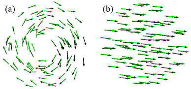
Figure 1: Snapshots of typical three-dimensional swarm patterns for 100 particles. (a) a rotational mill, and (b) a translating flock.

Most notably, despite being the dominant steady state in two dimensions, the single rotating mill shown in Fig. 1(a) is not a true three-dimensional steady state. Although particles may settle into identifiable mills, extensive simulations performed on a variety of initial conditions show that a mill in three dimensions will eventually acquire a non-zero center-of-mass velocity and evolve into a flock as shown in Fig. 1(b). In Fig. 2(a), we plot the state indicator $I_{\rm s}$ defined in the Appendix to characterize the swarming pattern. A value of $I_{s}=+1$ represents a perfect unidirectional flock, $I_{s}=0$ a random collection of particles, and $I_{s}=-1$ a perfect rotating mill. The red curve in Fig. 2(a) shows particles settling into a transient mill for a lengthy period of time before evolving into a translating flock; in contrast, the blue curve shows particles forming a flock without first assembling into a long-lived mill. In the latter case $I_{s}$ can first decrease before rising back to $I_{s}\approx 1$.

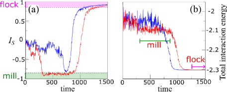
Figure 2: (a) Three-dimensional simulations of Eqs. 1 without hydrodynamic interactions. The classifier of swarming patterns $I_{s}$ is defined in the Appendix. The red curve denotes a swarm that first forms a mill before turning into a uniformly translating flock, while the blue curve shows particles evolving into a flock without first forming a mill. We empirically set thresholds $I_{s}\leq-0.85$ (green) to signal mills and $I_{s}\geq 0.85$ (magenta) to identify migrating flocks. We require a swarm to maintain the $I_{s}$ value in either the two ranges for a period of $100$ time units or more to be classified as a mill or flock. This criterion corresponds roughly to the time for a particle to circle a mill at least 10 times. (b) The total interaction energy $\sum_{i,j}\Phi\left(|{\bf r}_{i}-{\bf r}_{j}|\right)/2$ corresponding to the two simulations above. The translating flock has a lower interaction energy than the mill.

To understand how mills and flocks develop in three dimensions, in Fig. 2(b) we plot the evolution of the total interaction energy ${1\over 2}\sum_{i,j}\Phi\left(|{\bf r}_{i}-{\bf r}_{j}|\right)$ associated with the two simulations in Fig. 2(a), showing a lower total energy for the flock state. Note that when assembled into flocks, particles settle into positions that correspond to the global minimum of the total potential energy. In contrast, when assembled into mills, only a local minimum of the total potential energy is reached. In this case the net interaction force on each particle provides the centripetal force necessary to sustain the rotational movement. Although its energy is lower, for particles starting from random initial conditions, a flock may be kinetically less accessible than a mill. A mill is a state of local coherence, where particles match velocities with their close neighbors only, as opposed to a flock where global coherence arises from all particles moving in unison. As a result, three-dimensional mills often emerge first out of a randomized configuration. For the same reason, two-dimensional mills are not only stable at steady-state, but also dominate over flocks. However, three-dimensional mills are unstable since they slowly acquire a translational momentum along the rotational axis aligned with the third direction. As particle velocities gradually become aligned with this translational momentum, the rotational unit turns into a spiral with continuously reduced angular speed, finally settling into an equilibrium lattice formation migrating at a uniform velocity. This effect cannot arise in two dimensions.

Swimmer-induced fluid flow ${\bf u}_{\rm s}$ – We now investigate how patterns mediated by the ${\bf u}_{\rm s}$ flow field alone differ from those described in the fluid-free case above. In general, the extensional flow generated in the reference frame of a puller ($G<0$) converges along the direction of motion and diverges along the perpendicular direction. Pusher-generated ($G>0$) extensional flows move in the opposite direction, diverging along the direction of motion and converging laterally. As a result, pullers tend to flatten existing flocks into oblate shapes while pushers tend to longitudinally stretch them into prolate shapes. These deformed flocks are depicted in Fig. 3 for an opaque fluid.

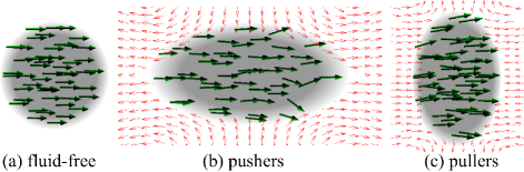
Figure 3: Snaphots of $50$-particle simulations showing the deformation of three-dimensional flocks by interacting with ${\bf u}_{\rm s}$ arising in opaque fluids ($\lambda=1$) when ${\bf u}_{\rm p}$ is absent. (a) For reference, we show the stable spherically shaped flock arising in the fluid-free case. This stable spherical flock is used as the initial conditions for both of the other two simulations before fluid interactions from ${\bf u}_{\rm s}({\bf r})$ are switched on. (b) A transient prolate flock forms when $G=0.15$ (pusher). (c) A transient oblate flock arises when $G=-0.15$ (puller). The red arrows indicate the direction of ${\bf u}_{\rm s}$ in the frame of the flock center-of-mass. In these simulations, the prolate flock is transitioning into a recirculating “peloton,” while the oblate flock is transitioning into a random blob. These deformed flocks are stable only if $|G|$ is small, but with much less distortion. The emergence of pelotons and random blobs is described below.

In clear fluids ($\lambda=0$), the energy of a swarm dissipates significantly through the fluid drag term, slowing particle motion and reducing ${\bf u}_{\rm s}$. For very large dimensionless drag $\gamma\gg 1$, the motion of both pushers and pullers is arrested and ${\bf u}_{\rm s}\to 0$. For intermediate $\gamma$, pushers align into prolate flocks and move at a reduced speed of approximately $\sqrt{1-\gamma}$; pullers also move at a reduced speed, but mostly randomly without any spatial order. The $\gamma\to 0$ limit is the fluid-free case.

We observe a more diverse set of swarm morphologies in opaque fluids ($\lambda=1$) where the self propulsion term ${\bf f}_{\rm M}$ imparts sufficient energy to the particles to keep them moving at their preferred self-propulsion speed relative to the background flow. In this case, the oblate/prolate deformation of flocks is more pronounced than in clear fluids. In Fig. 4(a) we show the time evolution of 50 particles for $\left|G\right|=0.096$. The red (blue) curves represent pullers (pushers). For reference we also plot the fluid-free case ($G=0$) in the green curve. For such small $G$, pusher-generated flows suppress the transient milling seen in the fluid-free case leading to a stable prolate flock. However, unlike the fluid-free case, pusher-generated flocks are not perfect and $I_{s}\approx 0.75<1$. Here, the spatial-temporal variations in ${\bf u}_{\rm s}$ impart fluctuations to the direction of particle movement, preventing the formation of a perfectly aligned flock. Puller-generated flows, on the other hand, allow for the formation of permanent mills: the mill-to-flock transition that occurs in the fluid-free case is blocked by the fluctuating flow field allowing mills to be long-lived.

Since the flow disturbance may be considered as a form of noise, our findings are consistent with previous reports of noise-induced flock-to-mill transitions in three dimensions Strefler et al. (2008); Romanczuk et al. (2012). The latter show hysteresis in swarm morphology as a function of the noise amplitude, a feature which we also observe with pullers as the thresholds in $G$ between a flock and random blob depend on whether $G$ is increased or decreased. In addition, we note that disturbances induced by ${\bf u}_{\rm s}$ lead to particles occasionally deviating from their circulating trajectories and to a striking intermittent disintegration and re-assembling of mills, a phenomenon that has not been reported in noise-induced flock-to-mill transitions. In Fig. 4(b), we conduct a more thorough investigation of long-time swarming patterns by varying $\left|G\right|$ for pullers (blue) and pushers (red). Pushers assemble into flocks as $G$ increases, but patterns are increasingly disturbed by ${\bf u}_{\rm s}$, leading to decreased $I_{s}$.

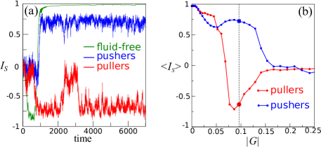
Figure 4: (a) Time-dependent swarm morphologies starting from random initial conditions. Pusher swarms ($G=0.096$, blue curve), evolve directly towards a fluctuating flock, while puller swarms ($G=-0.096$, red curve) assemble into rotating mills; the latter persists indefinitely but is intermittently interrupted by bursts of randomness. For comparison, we also plot the fluid-free case ($G=0$, green curve), where particles transiently form a mill before eventually assembling into a flock. (b) Long-time formations ($t>2000$) of pushers and pullers with different $G$ values. The indicator $\langle I_{s}\rangle$ is averaged for all time steps between $2000\leq t\leq 3000$ and over ten simulations. For pullers, persistent mills only occur approximately in the range of $0.07\leq G\leq 0.1$; below this range, flocks dominate, similarly to the fluid-free case; above this range, the swarm is in a permanent random state. Pushers always assemble into flocks; for large $G$, however, the flow field induces a peloton-like movement within the flock, which pushes $I_{s}$ towards zero.

For larger $G$, ${\bf u}_{\rm s}$ is strong enough to induce a novel “peloton”-like movement, where leading particles continuously recirculate toward the back end of the flock, as depicted in Fig. 5. When assembled into a peloton, $I_{s}$ drops to nearly zero, although the majority of particles are still aligned. Pullers on the other hand tend to keep milling as $\left|G\right|$ increases rather than transition to a flock. Here $I_{s}\approx-1$. For very large values of $\left|G\right|$ the strong flow field prevents even mills from forming, and particle movement remains random. Overall, our results suggest that pusher-generated flow fields generally promote particle velocity ordering along a common direction but that an orthogonal component of the flow prevents perfect alignment for small $G$ and ultimately to particles recirculating for large $G$. Puller-generated flow fields instead introduce more randomness preventing the mill to flock transition for small $\left|G\right|$ and completely preventing a mill from forming for larger $\left|G\right|$.

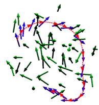
Figure 5: A snapshot of a peloton-like formation for $G=0.15$. Particle positions and velocities are represented by the green arrows, while the blue arrows connected by the red-dashed line track one particular particle for $15$ steps prior to the snapshot. The selected blue particle is initially near the leading edge of the flock, gets swept aside by the surrounding flow field, and finally rejoins the flock near the back end.

Physical force-induced fluid flow ${\bf u}_{\rm p}$ – We now examine the effects of ${\bf u}_{\rm p}$ on swarm dynamics by setting $G=0$ and analyze how patterns differ when compared to those arising in the fluid-free case. For a clear fluid $(\lambda=0)$ our simulations reveal that at steady state particles either stop or assemble into a flock. The resulting speed can be evaluated by balancing self-propulsion with drag, yielding a dimensionless flock speed $\sqrt{1-\gamma}$ for $\gamma\leq 1$ and $0$ for $\gamma>1$, which are both confirmed by simulations. In physical units, the friction threshold for immobilizing a flock is $6\pi\eta a>\alpha$. Hydrodynamic coupling in a viscous clear fluid simply slows or stops translational flock motion. Note that in the $a\to 0$ point-particle limit, drag is negligible and swarming in a clear fluid reduces to the canonical fluid-free problem.

Figure 6: Swarm patterns in an opaque fluid as $\eta$ is varied. Each point is an average over 100 simulations each initialized with random conditions. (a) Probability of transient mill formation for $\eta\geq 1.2$. Although in this high viscosity regime all initial conditions lead to uniformly translating flocks, the probability of first forming a transient mill decreases with decreasing $\eta$. (b) Probability of permanent flock formation for $\eta\leq 2$. In this low viscosity regime steady-state flocks are no longer the only final outcome when $\eta<1.2$. Other possible configurations are mill-like structures and random blobs.

As with swimmer-induced flows, the opaque fluid case is much more interesting. Here steady-state configurations depend nontrivially on the dimensionless viscosity $\eta$ (defined in the Appendix) which measures ratio of the fluid momentum relaxation time to the time scale of the particle movement, thus representing an effective Deborah number for the problem Reiner (1964); Lauga (2009). The parameter $\eta$ appears in Eq. 8 through ${\bf u}_{\rm p}({\bf r})$ in Eq. 7 and through $\gamma=6\pi\eta a$. We assume small particles and neglect this latter drag interaction. As can be seen from Eq. 7, ${\bf u}_{\rm p}$ decreases with $\eta$ so that as $\eta$ increases the dynamics resembles that of the fluid-free case. Indeed, we find that for $\eta>1.2$, flocks are the only stable steady-state solution for all random initial conditions used, similar to the fluid-free case. However, transient mills can form before the permanent flock is assembled, with the probability of transient mills occurring decreasing with $\eta$. As shown in Fig. 6(a), for $\eta=100$ particles form mills before finally settling into flocks for about $50\%$ of the random initial conditions used; this ratio drops to about $20\%$ at $\eta=1.2$.

Below $\eta\approx 1.2$, swarms experience a qualitative change in behavior and flocks are no longer the only long-lived steady-state. Fig. 6(b) shows that the probability of final flock formation decreases from unity at $\eta\approx 1.2$ to zero at $\eta\approx 0.1$. In this intermediate range of $\eta$, two other long-lived configurations can arise: a mill-like formation as shown in Fig. 7(a), and a perpetual random blob. Unlike the annular- or toroidal-shape of a classical mill, the hydrodynamically-mediated three-dimensional mill-like structure has a central core filled with randomly moving particles. As the dimensionless viscosity decreases from $\eta\approx 1.2$, the randomly-moving core particles in a mill-like swarm expand their boundaries and eventually swallow the coherent part of the mill. The resulting pattern is a perpetual random blob without any identifiable spatial order. Finally, for $\eta\lesssim 0.1$, swarms immediately collapse into the above described blob of perpetual random movement. All possible swarming patterns are listed in Table 1 as a function of the dimensionless viscosity $\eta$. A viscous flow ${\bf u}_{\rm p}$ thus allows for the emergence of persistent mill-like structures not observed in the absence of fluid flows.

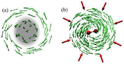
Figure 7: (a) A stable mill-like formation of 100 particles induced by hydrodynamic interactions in an opaque fluid with $\eta=0.7$. The gray shading delineates a disordered core that grows as $\eta$ is decreased. (b) A transient mill of 250 particles with an empty core in an opaque fluid. Such transient mills may arise when $\eta>1.2$. The induced flow field is indicated by the red arrows and converges toward the central core along the plane of rotation. To balance the influx, a jet along the axis of rotation ejects the fluid from the central core. The jet is normal to the page and depicted by red arrow in panel (b).

	intermediate $t$	long $t$
$\eta>1.2$	mill or flock	flock only
	mill or flock	flock
$0.1<\eta<1.2$	mill-like or random	mill-like
	random	random
$\eta<0.1$	random	random

Table 1: Swarming structures observed in simulations for intermediate and long ($t>3000$) times under the ${\bf u}_{\rm p}$ flow field and as a function of the dimensionless fluid viscosity $\eta$. Steady state configurations take longer to assemble here than under ${\bf u}_{\rm s}$. In the fluid-free case only flocks arise at long times. A moderately viscous fluid allows for the emergence of permanent mill-like structures and random blobs.

We can also examine the induced flow fields in relation to particle velocities, and how they may drive transitions among various swarm morphologies. Starting from a high-$\eta$ transient mill regime ($\eta\gtrsim 1.2$), Fig. 7(b) qualitatively indicates the instantaneous direction of the hydrodynamic velocity field ${\bf u}_{\rm p}({\bf r})$ (red arrows) induced by a mill-like formation of $250$ particles. In a transient mill, the net particle-particle interactions provide the centripetal force that sustains rotation. This net force is imparted on the fluid, inducing an inward flow along the plane of rotation. The incompressible fluid is then ejected outward along the rotational axis, resembling a “jet” emanating from the center of an accretion disk.

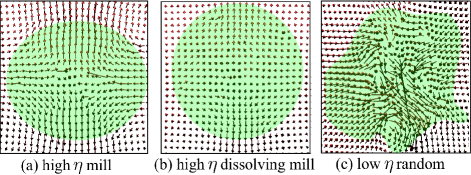
Figure 8: Fluid velocity fields ${\bf u}_{\rm p}({\bf r})$ associated with particle swarms concentrated within the green shaded regions. (a) For large $\eta$, an early flow field resembles a jet. (b) At longer times the jet is eventually disrupted and a flock forms. (c) For very low $\eta<0.1$, the disordered core region of a transient mill-like formation will always expand eventually leading to a random blob.

This outward jet entrains particles that wander into the core region, slowly disrupting the mill. Entrainment arises through the self-propulsion term ${\bf f}_{\rm M}$, and if appreciable, through viscous drag. Moreover, the inward flow on the rotational plane effectively extends the interaction range among particles, driving the system into a minimum-energy flock state. As $\eta$ is decreased, the induced Stokes accretion flow increases and drives more particles into the core of the mill. Particle motion then becomes randomized, disrupting the outward jet and ultimately hindering the mill-to-flock transition that would otherwise occur smoothly. Swarms can thus be trapped in the mill-like formation shown in Fig. 7(a) indefinitely as listed in Table 1. At even lower values of $\eta$, coherence is lost by an expanding disordered core region. The fluid flow fields observed under different regimes of $\eta$ are plotted in Fig. 8.

Combined effects of ${\bf u}_{\rm s}$ and ${\bf u}_{\rm p}$ – In light of the above discussions, we now consider the effects of superimposing the two fields so that ${\bf u}({\bf r})={\bf u}_{\rm s}({\bf r})+{\bf u}_{\rm p}({\bf r})$. The magnitudes of ${\bf u}_{\rm s}$ and ${\bf u}_{\rm p}$ can be varied independently, and are controlled by $G$ and $\eta$, respectively. In clear fluids ($\lambda=0$), the two flows combine to reduce flock speed to $\sqrt{1-\gamma}$, except in the case of very strong puller flows (large $|G|$) that prevent particles from aligning into flocks and lead to a random blob.

Fig. 9 shows the phase diagram in ($G,\eta$)-space of stable swarm structures arising in opaque fluids $(\lambda=1)$. In opaque fluids for small values of $\eta$, ${\bf u}_{\rm p}$ dominates ${\bf u}_{\rm s}$ and swarms assemble into a random blob. As $\eta$ increases, ${\bf u}_{\rm p}$ decreases and the effects of ${\bf u}_{\rm s}$ become more pronounced, prevailing for large $\eta$. In this case, flows generated by strong pullers (very negative $G$) still favor the emergence of a random blob. However, upon increasing $G$ fluctuating transient mills arise. As $G$ keeps increasing, flows generated by pushers favor the formation of fluctuating flocks until for very large $G$ pelotons emerge. As can be seen in Fig. 9, mill-like patterns exist only when $G=0$, suggesting that such structures are easily disrupted or prevented from forming by ${\bf u}_{\rm s}$.

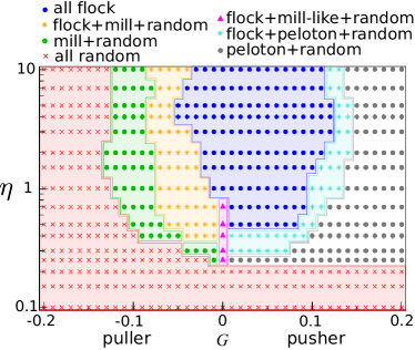
Figure 9: Phase diagram in $(G,\eta)$-space delineating possible persistent structures ($t>3000$) in the presence of the total flow field ${\bf u}({\bf r})={\bf u}_{\rm s}({\bf r})+{\bf u}_{\rm p}({\bf r})$. Each point summarizes the possible final morphologies from $10$ simulations. Flocks are more likely to emerge for large $\eta$, and random blobs are more prominent for small $\eta$. For pullers ($G<0$), mills may appear with increasing $\left|G\right|$, but random blobs dominate at large $\left|G\right|$. The flow ${\bf u}_{\rm s}$ generated by weak pushers ($G\gtrsim 0$) promotes particle alignment and flock formation. For even larger $G$, flocks exhibit peloton-like movement.

Summary and Conclusions

In the absence of hydrodynamic coupling, our extensive numerical simulations revealed that three-dimensional swarms exhibit much less diversity than in two dimensions. This is due to the additional dimension that provides a pathway for a variety of stable two-dimensional patterns to transform into energy-minimizing, uniformly translating flocks in three dimensions. We then carefully explored the effects of hydrodynamic coupling on three-dimensional swarming by deriving a discrete model of self-propelled interacting swimmers in an incompressible zero-Reynolds-number Newtonian fluid.

An important distinction in the source of fluid flow is made. Under a force-free assumption, particle swimming (or squirming Ishikawa et al. (2006)) can only generate flows that decay as $1/r^{n},n\geq 2$. When direct action-at-a-distance physical forces (electrostatic, magnetic, gravitational) arise between self-propelled particles, an additional Oseen flow decaying as $1/r$ can arise Happel and Brenner (1965); Español et al. (1995); Batchelor (2000). Thus, even short-ranged pairwise physical forces can generate longer-ranged fluid motion enhancing particle interactions and greatly affect swarm morphology.

In clear three-dimensional fluid environments we find that only flocks arise, similar to the fluid-free scenario, albeit with particles moving at reduced speed. Note that our patterns emerge through direct interactions among particles, in contrast to the ones observed in previous studies of infinite or confined systems of swimmers coupled only via the fluid drag Baskaran and Marchetti (2009). The latter models include particle density as a fixed, prescribed parameter, so that high-density particles can be forced to interact out of equilibrium. As a result, density-dependent transitions and states, such as nematic orders, may arise. On the contrary, we consider a finite number of particles in an infinite domain, where local particle density is determined by particles collectively minimizing the interactions amongst them, favoring the low-energy flock formation. In opaque fluids, pusher generated flows accelerate particle alignment and suppress the emergence of metastable mills seen in the fluid-free case. Puller-generated flows, conversely, hinder particle velocity alignment, allowing transient mills to persist within certain viscosity ranges. Sufficiently strong puller flows disrupt any spatial order. Flows generated by particle-particle interactions kinetically accelerate the mill-to-flock transition. In high-viscosity opaque fluids, the hydrodynamic flow fields can form an accretion disk/jet structure associated with mills and entrain the self-propelled particles leading to quicker dissolution of the mill itself. However, in opaque fluids of intermediate viscosity, stronger hydrodynamic interactions may kinetically block the mill-to-flock transition, allowing a mill-like formation to form and persist. At even lower fluid viscosity $\eta$, swarms are completely chaotic.

When both swimming- and force-induced flows are present, steady-state configurations depend on the relative strength between the two flows. Mill-like formations are absent. Our main results pertain to viscous steady-state Stokes’ flows, but we derive time-dependent interaction-induced fluid velocities and inertial interactions arising in potential flows in the Appendix. We used the Morse potential in our simulations to provide a mechanistic picture of collective behavior of three-dimensional swarms and found a rich phase diagram of patterns; however, the structure of our fluid-coupled swarming model is sufficiently general that any effective interaction potential can be used provided the its social or physical underpinnings are carefully delineated.

Our swarming model can be further refined by addressing more microscopic fluid coupling mechanisms. In our model, Eq. 5 defines a stroke period-averaged flow field and Eq. 1 describes hydrodynamic coupling under the period-averaged flow assumption. However, the phase difference of the microscopic strokes between two swimmers has been shown to actively affect the interaction in unexpected ways, leading to attraction, repulsion, or oscillations Pooley et al. (2007). How these subtle swimmer-induced pairwise interactions Ishikawa et al. (2006); Pooley et al. (2007) influence the collective behavior of swarms remains to be investigated. Finally, we have not considered the effects of external potentials. Our derivation of the fluid coupling mechanisms suggest the possibility of more new structures depending on whether the external potential derives from social interactions that influence self-propulsion (e.g., chemotaxis) or physical ones (e.g., gravity) that result in body forces on the fluid. The physical and mathematical structure of our fluid-coupled kinetic models provide a basis for future investigation of these extensions.

Appendix A Non-dimensionalization

The non-dimensional parameters used in Eq. 8 are defined as

$$\begin{array}[]{lll}{\bf r}^{\prime}=\displaystyle{\frac{\sqrt{\alpha\beta}}{m}{\bf r}},&t^{\prime}=\displaystyle{\frac{\alpha}{m}t,}\\ \\ {\bf v}_{i}^{\prime}=\displaystyle{\sqrt{\frac{\beta}{\alpha}}}{\bf v}_{i},&{\bf u}^{\prime}=\displaystyle{\sqrt{\frac{\beta}{\alpha}}}{\bf u},&\gamma^{\prime}=\displaystyle{\frac{\gamma}{\alpha}},\\ \\ \rho^{\prime}=\displaystyle{\frac{m^{2}}{\sqrt{\alpha^{3}\beta^{3}}}}\rho,&\eta^{\prime}=\displaystyle{\frac{m}{\sqrt{\alpha^{3}\beta}}}\eta,&G^{\prime}=\displaystyle{\frac{\alpha\beta}{m^{2}}}G,\\ \\ \Phi^{\prime}=\displaystyle{\frac{\beta}{\alpha m}}\Phi,&p^{\prime}=\displaystyle{\frac{m^{2}}{\sqrt{\alpha^{5}\beta}}}p,&\\ \\ C_{a}^{\prime}=\displaystyle{\frac{\beta}{\alpha m}}C_{a},&C_{r}^{\prime}=\displaystyle{\frac{\beta}{\alpha m}}C_{r},&\\ \\ \ell_{a}^{\prime}=\displaystyle{\frac{\sqrt{\alpha\beta}}{m}}\ell_{a},&\ell_{r}^{\prime}=\displaystyle{\frac{\sqrt{\alpha\beta}}{m}}\ell_{r}.\end{array}$$ (S8)

Appendix B Time-dependent Stokes flow

We assume $\nu\rightarrow 0$ for the dimensionless Stokes Eq. 8 of the main text and conduct our investigation at the quasistatic limit. More generally, the time-dependent velocity field can be expressed as

$${\bf u}({\bf r}_{j},t)=\frac{1}{\rho}\sum_{i\neq j}\int_{0}^{t}\mbox{d}t^{\prime}{\bf T}({\bf r}_{i}-{\bf r}_{j};t-t^{\prime})\cdot{\bf f}_{i},$$ (S9)

where $\rho$ is the mass density of the embedding Newtonian fluid and ${\bf T}$ is the three-dimensional dynamic Oseen tensor given by Español et al. (1995)

$$\begin{array}[]{rl}{\bf T}({\bf r},t)&\displaystyle=\int{\mbox{d}^{3}{\bf k}\over(2\pi)^{3}}e^{-\nu k^{2}t+i{\bf k}\cdot{\bf r}}\left[{\bf I}-\hat{{\bf k}}\hat{{\bf k}}\right]\\[13.0pt] &\displaystyle=p(r,t){\bf I}-q(r,t)\hat{{\bf r}}\hat{{\bf r}},\end{array}$$ (S10)

with

$$\begin{array}[]{l}\displaystyle p(r,t)=\left(1+{2\nu t\over r^{2}}\right)f(r,t)-{g(r,t)\over r^{2}}\\[13.0pt] \displaystyle q(r,t)=\left(1+{6\nu t\over r^{2}}\right)f(r,t)-{3g(r,t)\over r^{2}}\\[13.0pt] \displaystyle f(r,t)={1\over(4\pi\nu t)^{3/2}}\exp\left[-{r^{2}\over 4\nu t}\right]\\[13.0pt] \displaystyle g(r,t)={1\over 4\pi r}{\rm erf}\left({r\over\sqrt{4\nu t}}\right).\end{array}$$ (S11)

In the quasistatic limit, the Oseen tensor is

$${1\over\rho}{\bf T}({\bf r},t)\approx{1\over 8\pi\eta r}\left[{\bf I}+\hat{{\bf r}}\hat{{\bf r}}\right]\delta(t),$$ (S12)

which is used in Eq. 7 to provide an analytic form of the velocity field. The solution to the pressure field $p({\bf r},t)$ is also given; however, its effect on swimmers is ignored since its gradient is negligible across the size $a\to 0$ of small particles.

Appendix C Potential flow

As derived in Blake (1988), the fluid velocity potential $\phi({\bf r})$ at a location ${\bf r}$ from an accelerating spherical particle of radius $a$ can be approximated in the far-field $|{\bf r}|\gg a$ limit by the formula

$$\phi\left({\bf r},t\right)\sim-\frac{m\left(t\right)}{4\pi\left|{\bf r}\right|}-\frac{\mathbf{d}\left(t\right)\cdot{\bf r}}{4\pi\left|{\bf r}\right|^{3}}+\mathcal{O}\left(\left|{\bf r}\right|^{-3}\right),$$ (S13)

where

$$m\left(t\right)=\oint_{\partial V}\nabla\phi\cdot\mathrm{d}\mathbf{S},$$ (S14)

and

$$\mathbf{d}\left(t\right)=\oint_{\partial V}\phi\mathrm{d}\mathbf{S}+\oint_{\partial V}\mathbf{r}\nabla\phi\cdot\mathrm{d}\mathbf{S}$$ (S15)

are obtained by integrating over the boundary $\partial V$ of the spherical volume $V$ of the source object. The near-field $\phi$ in the integrands depends on the shape and swimming mechanism of the source object. Let us consider the simplest case of solid spherical particles moving through an inviscid fluid. For a lone particle of radius $a$ traveling at a velocity ${\bf v}$ as illustrated in Fig. 10, we may derive the fluid velocity potential in the laboratory frame as follows

$$\phi({\bf r})=-v\frac{a^{3}}{2\left|{\bf r}\right|^{2}}\cos\theta,$$ (S16)

where $v=\left|{\bf v}\right|$, ${\bf r}$ is the a spatial position relative to the center of the particle, and $\theta$ is the angle between ${\bf r}$ and ${\bf v}$.

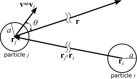
Figure 10: Hydrodynamic interactions due to potential flow. Eqs. S13-S16 express the approximated fluid potential at an arbitrary far-field location caused by the acceleration of a particle at ${\bf r}_{j}$. Eq. S21 gives the force induced by the fluid potential on a particle at ${\bf r}_{i}$.

Substituting Eq. S16 into Eqs. S14 and S15, we obtain

$$\begin{array}[]{l}m\left(t\right)=0,\quad\mbox{and}\quad\mathbf{d}\left(t\right)=2\pi a^{3}{\bf v}\left(t\right).\end{array}$$

As a result, the far-field fluid velocity potential of the moving sphere is

$$\phi\left({\bf r},t\right)\sim-\frac{a^{3}{\bf v}\left(t\right)\cdot{\bf r}}{2\left|{\bf r}\right|^{3}},$$ (S16)

Let us now calculate the force induced by a moving particle at position ${\bf r}_{j}$ on an identical particle at a position ${\bf r}_{i}$. We assume that $\left|{\bf r}_{i}-{\bf r}_{j}\right|\gg a$, so that the far-field approximation is appropriate. From the Euler equation of inviscid flow, we know that the fluid velocity potential $\phi$ induces a pressure

$$p=p_{0}-\rho\frac{\partial\phi}{\partial t}-\frac{1}{2}\rho\left|{\bf u}\right|^{2},$$ (S17)

where $\rho$ is the fluid density, ${\bf u}=\nabla\phi$ is the fluid velocity, and $p_{0}$ is an arbitrary reference point of the pressure. The resultant force on a spherical object is found from integrating the pressure variation over its surface:

$${\bf F}_{\mathrm{p.f.}} \displaystyle=\oint_{\partial V}p\mathrm{d}\mathbf{S}$$

$$\displaystyle=-\oint_{\partial V}\rho\frac{\partial\phi}{\partial t}\mathrm{d}\mathbf{S}$$

$$\displaystyle=\frac{\rho}{4\pi}\frac{\mathrm{d}\mathbf{d}\left(t\right)}{\mathrm{d}t}\cdot\oint_{\partial V}\frac{\left({\bf r}-\mathbf{s}\right)}{\left|{\bf r}-\mathbf{s}\right|^{3}}\hat{\mathbf{s}}\mathrm{d}S.$$ (S18)

Here, ${\bf r}\equiv{\bf r}_{j}-{\bf r}_{i}$, $\mathbf{s}$ is a vector from the particle center to the particle surface, and $\hat{\mathbf{s}}\equiv\mathbf{s}/\left|\mathbf{s}\right|$. For a spherical particle of radius $a=\left|\mathbf{s}\right|\ll\left|{\bf r}\right|$, we use the approximation $\left|{\bf r}-\mathbf{s}\right|^{-3}\simeq\left|{\bf r}\right|^{-3}\left(1+3\left(\mathbf{s}\cdot{\bf r}\right)/\left|{\bf r}\right|^{2}\right)$ to find

$${\bf F}_{\mathrm{p.f.}}=\frac{\rho a^{3}}{3\left|{\bf r}\right|^{3}}\dot{\mathbf{d}}(t)\cdot\left[3\frac{{\bf r}{\bf r}}{\left|{\bf r}\right|^{2}}-\mathbf{I}\right].$$ (S19)

Substituting Eq. S15 into the above equation, we obtain

$${\bf F}_{\mathrm{p.f.}}=\frac{2\pi\rho a^{6}}{3\left|{\bf r}\right|^{3}}\dot{{\bf v}}(t)\cdot\left[3\frac{{\bf r}{\bf r}}{\left|{\bf r}\right|^{2}}-\mathbf{I}\right].$$ (S20)

Assuming there are $N$ identical particles, the potential flow induced force on particle $i$ is thus

$${\bf F}^{i}_{\mathrm{p.f.}}=\frac{2\pi\rho a^{6}}{3}\sum_{j\neq i}^{N}\frac{\dot{{\bf v}}_{j}(t)}{\left|{\bf r}_{j}-{\bf r}_{i}\right|^{3}}\cdot\left[3\frac{\left({\bf r}_{j}-{\bf r}_{i}\right)\left({\bf r}_{j}-{\bf r}_{i}\right)}{\left|{\bf r}_{j}-{\bf r}_{i}\right|^{2}}-\mathbf{I}\right].$$ (S21)

Note that the force is short-ranged, of the order $\mathcal{O}\left(\left|{\bf r}_{j}-{\bf r}_{i}\right|^{-3}\right)$. Moreover, its amplitude is proportional to $a^{6}$. As a result, the hydrodynamic interaction force induced by potential flows does not have significant impact on collective behavior particularly when $\rho$ and/or the volume fraction of particles is small. If $\rho$ is very large, the flow field imposes a repulsion between particles that encounter each other, potentially preventing them from forming a coherent structure.

Appendix D Indicator of the swarming states

Here we define a metric to describe the state of a swarm. This quantity will consistently distinguish between parallel flock, single rotating mill, and random swarms. To identify the parallel flock state, we note that all particles are moving at the same velocity as the Center-of-Mass (CM) velocity. To find the rotating mill state, we take advantage of the fact that all particles share the same axis of rotation. We combine these properties into a single quantity $I_{s}$ over the desired range $[-1,1]$ where $-1$ is associated with a perfect mill and $+1$ indicates a uniformly translating flock. The indicator $I_{s}$ is decomposed according to

$$I_{s}\equiv I_{\mathrm{flock}}-I_{\mathrm{mill}}.$$ (S22)

Given $N$ particles,

$$I_{\mathrm{flock}}\equiv 1-\frac{\sum_{i}\left|\mathbf{v}_{i}-\mathbf{v}_{\mathrm{CM}}\right|}{N\sqrt{\alpha/\beta}}.$$ (S23)

Note that $I_{\mathrm{flock}}=1$ for a perfect parallel flock and $I_{\mathrm{flock}}=0$ for a perfect mill. To define $I_{\mathrm{mill}}$ we first compute the rotational axis $\hat{\mathbf{\omega}}_{i}$ of particle $i$:

$$\hat{\mathbf{\omega}}_{i}\left(t\right)=\frac{\mathbf{v}_{i}\left(t\right)\times\mathbf{F}_{i}\left(t\right)}{\left|\mathbf{v}_{i}\left(t\right)\right|\left|\mathbf{F}_{i}\left(t\right)\right|}.$$ (S24)

where $\mathbf{F}_{i}$ is the force acting on particle $i$. We then evaluate the degree of alignment between all $\hat{\mathbf{\omega}}_{i}$ and define

$$I_{\mathrm{mill}}=\frac{\sum_{i}\sum_{j\neq i}\hat{\mathbf{\omega}}_{i}\cdot\hat{\mathbf{\omega}}_{j}}{N\left(N-1\right)}.$$ (S25)

Note that $I_{\mathrm{mill}}=1$ when the rotations of all the particles are perfectly aligned and $I_{\mathrm{mill}}=0$ when all particles are in a perfect parallel flock formation. Putting $I_{\mathrm{flock}}$ and $I_{\mathrm{mill}}$ together in $I_{s}$ (Eq. S22), we find $I_{s}=-1$ for a perfect mill and $I_{s}=+1$ for a perfect flock. Finally, since swarms are seldom in a perfect formation, we considered thresholds on $I_{s}$ as indicated in Fig. 2.

Distinguishing more subtly different structures is not always unequivocal using the metric $I_{s}$. In particular, we prescribe $I_{s}>0.5$ to indicate a flock and $I_{s}<0.5$ to indicate a peloton where there is more rotational movement from particle recirculation.

Appendix E Effects of changing interaction potentials

All the results presented in the main text were obtained using a fixed set of potential parameters $C_{r,a},\ell_{r,a}$. The primary effect of varying these parameters is to change the spatial size of swarms. For rotational mills, an increase in diameter is accompanied by a decrease in the magnitude of the centripetal force and weaker destabilizing flows. A larger swarm is also less sensitive to hydrodynamic effects since particles are spaced further apart, generating weaker interaction forces and hence weaker flows. In Fig. 11, we explore different potentials and test the robustness of flock formation in the low $\eta$ regime where the flock can be broken up by hydrodynamic interactions. Not surprisingly, for potentials that are more “H-stable” D’Orsogna et al. (2006); Chuang et al. (2007a), the probability of stable flock formation increases. While H-stability is an equilibrium property that is insensitive to hydrodynamics D’Orsogna et al. (2006); Chuang et al. (2007a), our results suggest that H-stable flocks are more resistant to hydrodynamic disruption.

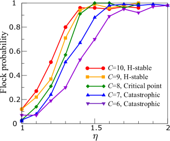
Figure 11: The dependence of stable flock formation probability on potential types and opaque medium viscosity. Here, we fix $\ell_{a}=1$, $\ell_{r}=0.5$ and vary $C\equiv C_{r}/C_{a}=6-10$ while keeping $C_{a}=100$. H-stable flocks are more robust against hydrodynamic disruption.