The galaxy luminosity function and the Local Hole

Abstract

Whitbourn & Shanks (2014) have reported evidence for a local void underdense by $\approx 15$% extending to 150-300h^-1Mpc around our position in the Southern Galactic Cap (SGC). Assuming a local luminosity function they modelled K- and r-limited number counts and redshift distributions in the 6dFGS/2MASS and SDSS redshift surveys and derived normalised n(z) ratios relative to the standard homogeneous cosmological model. Here we test further these results using maximum likelihood techniques that solve for the galaxy density distributions and the galaxy luminosity function simultaneously. We confirm the results from the previous analysis in terms of the number density distributions, indicating that our detection of the ‘Local Hole’ in the SGC is robust to the assumption of either our previous, or newly estimated, luminosity functions. However, there are discrepancies with previously published K and r band luminosity functions. In particular the r-band luminosity function has a steeper faint end slope than the $r_{0.1}$ results of Blanton et al. (2003) but is consistent with the $r_{0.1}$ results of Montero-Dorta & Prada (2009); Loveday et al. (2012).

1 Introduction

Our local galaxy clustering environment has recently assumed even greater importance with the discovery that the SNIa Hubble diagram can be fitted by a Universe with an accelerating expansion rate (Schmidt et al., 1998; Perlmutter et al., 1999). Given the finely tuned nature of the vacuum energy that is implied by cosmological explanations of the form of the Hubble diagram, (Carroll, 2001), there is clear motivation to look for other explanations for this observation. This has led to a variety of activity investigating whether the local expansion rate is faster than at larger distances due to the presence of a Local Hole or Void. Indeed, there have been claims of a local underdensity manifesting as a local rise in SNIa based measurements of $H_{0}$ (Zehavi et al., 1998; Jha, Riess & Kirshner, 2007). Although some authors attribute these results to systematics associated with dust (Conley et al., 2007) these results are consistent with other work where bulk flows out to $z<0.06$ are found using SNIa (Feindt et al., 2013; Colin et al., 2011; Wojtak et al., 2014) and the tension between local and CMB determinations of $H_{0}$ (Planck Collaboration et al. 2014 - XVI). Some of the work in this regard has even focused on non-Copernican models with the Local Group positioned at the centre of a large void (Clarkson & Maartens, 2010; Schwarz, 2012; Krasiński, 2014). Here we are investigating a simpler scenario where the Local Group is at the edge of an underdense region that covers much of the Southern Galactic Cap (SGC). Evidence for such a possibility has been presented by Shanks (1990), Zucca et al. (1997), Metcalfe et al. (2001, 2006), Busswell et al. (2004) and Frith et al. (2003); Frith, Outram & Shanks (2005); Frith, Shanks & Outram (2005); Frith, Outram & Shanks (2006).

Whitbourn & Shanks (2014, the compansion study to this paper, which we will refer to hereafter as Paper I) have also recently presented evidence for a local void with an $\approx 15$% under-density out to $\approx 150-300$h^-1Mpc. These authors used 6dFGS/2MASS and SDSS redshift surveys to probe the local region by modelling the $n(z)$ distributions from three large regions of sky covered by these surveys. They also used the $\overline{z}(m)$ technique of Soneira (1979) to make a Hubble diagram based on the redshift survey galaxies and showed that the data preferred a model that showed coherent bulk motion out to 150h^-1Mpc compared to a model where the galaxy motions recovered the CMB dipole within the survey region.

More recently Keenan et al. (2010, 2012); and Keenan, Barger & Cowie (2013), have compared galaxy counts and luminosity density at high and low redshift and reported evidence for a 300Mpc void with a 50% underdensity. Alternative probes than K-band galaxy surveys have also been used to study this hypothesis. In particular Böhringer et al. (2015) used the X-ray selected REFLEX II cluster survey. These authors find evidence for significant underdensities with conclusions broadly similar to those of Paper I.

In Paper I we traced the local $n(z)$ using techniques that assumed the form of the luminosity function (LF) from previous work. The assumed form was also inferred in the $r$ and $K$ bands from original observations of LF’s as a function of galaxy morphology/$B-V$ colour in the $B$ band. Here we return to the issue of the Local Hole now using maximum likelihood (ML) methods (Choloniewski, 1987; Efstathiou, Ellis & Peterson, 1988; Cole, 2011) that solve for the galaxy density run with redshift, $\phi(z)$, simultaneously with solving non-parametrically for the luminosity function. The only parameters needed are simple forms for the K-correction and evolution $K+E$ terms.

In particular, we begin by describing the techniques used in estimating the galaxy LF and the underlying density fields. We first report the $V/V_{max}$ results for the K-band and relate these results to the number count slopes reported in Paper I. We then show the K-band LFs and compare to the Metcalfe et al. (2001, 2006) LF assumed in determining the density profiles presented in Paper I. We proceed by presenting the density profiles estimated in conjunction with the LF’s using ML methods. We also include similar results for the r band SDSS sample.

Throughout this paper we use a flat $\Lambda$ cold dark matter ($\Omega_{\Lambda,0}=0.7,\Omega_{m,0}=0.3$) cosmology with Hubble constant $H=100$h kms^-1 Mpc^-1 with $h=0.7$.

2 Techniques

We now briefly describe the methods of estimating the galaxy LF used in this paper. Unless otherwise stated we have estimated non-parametric LFs using binsizes of d$M=0.5$ and d$\mu=0.25$.

2.1 Non-parametric luminosity function estimation

2.1.1 $V_{max}$ luminosity function

We have used the standard $1/V_{max}$ estimator (Kafka, 1967; Schmidt, 1968). This method assumes a homogeneous model and estimates the LF as

$$\phi(M)=\sum_{i}^{N}\frac{1}{V_{i,max}}W(M_{i}-M),$$ (1)

where $V_{max}$ is the comoving volume associated with the maximum redshift this galaxy could be observed and $W(M_{i}-M)$ is a window function describing the binning d$M$ assumed for the LF, i.e.

$$W(M_{i}-M)=\begin{cases}1&\text{if }-\textrm{d}M/2\leq(M_{i}-M)\leq\textrm{d}M/2\\ 0&\text{if else}\end{cases}$$ (2)

One advantage of this method is the relative ease with which it can be extended to allow weighting of galaxies. This can be achieved by replacing the unity argument of the window function for galaxies in the absolute magnitude bin d$M$ by a weighting factor (Ilbert et al., 2005). We have used the magnitude dependent completeness factor described in appendix II of Paper I, i.e. $1/f(m_{i})$ where $f(m_{i})$ is the spectroscopic success function described in Paper I. We can account for a bright magnitude limit by replacing $V_{max}$ by $V_{max}-V_{min}$ in the denominator of equation (1) since this is now the volume over which the survey is complete at this absolute magnitude.

Whilst this estimator of the LF is minimum-variance and ML it is also biased as it assumes homogeneity and will therefore be affected by LSS (Felten, 1976). Importantly, other LF estimators are unaffected by LSS variations hence the difference between this LF estimator and the others is therefore reflective of the presence of LSS. Although this method offers an estimate of the global normalisation of the LF, no estimate of the density run $\phi(z)$ is available from this binned LF estimator.

2.1.2 NPML: Choloniewski-Peebles luminosity function

An alternative approach is a non-parametric maximum likelihood (NPML) method due to PJE Peebles (private communication) and Choloniewski (1986). The NPML method assumes separable densities $\rho_{i}$ and LF $\phi_{j}$ with Poisson distribution in the brightness-distance modulus plane $(M,\mu)$. The probability for $n_{i,j}$ galaxies to occupy the $i,j$th brightness-distance modulus bin is

$$p(N=n_{ij})=\frac{\exp^{-\rho_{i}\phi_{j}}(\rho_{i}\phi_{j})^{n_{ij}}}{n_{ij}!}.$$ (3)

Differentiating the log likelihood formed from these probabilities gives estimates that can be solved iteratively (Takeuchi, Yoshikawa & Ishii, 2000)

$$\rho_{i} =\sum_{j}n_{ij}/\sum_{j}\phi_{j}$$ (4)

$$\phi_{j} =\sum_{i}n_{ij}/\sum_{i}\rho_{i}$$ (5)

On the basis that the cross terms are zero the Fisher matrix errors are simply

$$\sigma_{\rho_{i}} =\frac{\rho_{i}}{(\sum_{j}n_{ij})^{1/2}}$$ (6)

$$\sigma_{\phi_{j}} =\frac{\phi_{j}}{(\sum_{i}n_{ij})^{1/2}}$$ (7)

This is an ML method which is independent of inhomogeneity (Choloniewski, 1986). Furthermore, it also offers an estimate of the global normalisation of the LF and the density run $\phi(z)$. However the method’s accuracy is dependent on galaxies being Poisson distributed across the brightness and distance modulus binning. The validity of this assumption is improved by smaller bin sizes but at the expense of possible bias (which increases with smaller bin sizes; Choloniewski 1986). We have used d$M=0.5$, d$\mu=0.25$ for the K band and d$M=0.2$, d$\mu=0.2$ for the r band.

2.1.3 $C^{-}$ luminosity function

We have also used the $C^{-}$ method of Lynden-Bell (1971) as updated by Choloniewski (1987). Here the distribution of galaxies in the $(M,\mu)$ plane is used to infer a binned non-parametric LF.

For a sample sorted from brightest to faintest we construct the $C^{-}$ statistic as (Lynden-Bell, 1971) follows,

$$C^{-}=\sum_{i}^{M<M_{i}}\ \sum_{m_{b}-M_{i}\leq\mu_{j}}^{\mu_{j}\\ \leq m_{f}-M_{i}}w_{ij},$$ (8)

where $w_{ij}$ is the weight of each galaxy which can be used to account for incompleteness (Ilbert et al., 2005). We have again accounted for incompleteness as $w_{ij}=1/f(m_{ij})$ where $f(m_{ij})$ is the spectroscopic success function described in Paper I. The summation is defined by the ranges associated with the faint ($m_{f}$) and bright ($m_{b}$) magnitude limits.

These $C^{-}$ coefficients can then be related to the cumulative LF $\Phi(M)$ through a recursion relation. This method for estimating the cumulative LF was modified by Choloniewski (1987) who extended it to enable an estimate of the underlying LF with a global normalisation and a density profile. It is this version of the estimator that we use in this study. Further discussion of the method can found in Choloniewski (1987), Willmer (1997) and Takeuchi, Yoshikawa & Ishii (2000).

2.1.4 Joint SWML method

The Efstathiou-Ellis-Peterson (EEP) estimator is a ML estimate which maximises the probability of selection (Efstathiou, Ellis & Peterson, 1988):

$$p=\frac{\phi(M)}{\int_{M_{b}(z)}^{M_{f}(z)}\phi(M)dM}.$$ (9)

Here the bounds on the integral are defined by the selection criteria of the survey. We can therefore calculate the likelihood, $\mathcal{L}=\prod_{i}^{N}p_{i}$, over binned values of the LF to find the ML estimator. This binning of the LF requires the use of step-functions in describing the ML solution. This step-wise approach has led to the estimator being described as the Step-Wise ML method (SWML). This method has been updated by Cole (2011) to jointly estimate the global normalisation, density profiles and the LF (JSWML). It is this JSWML version of the non-parametric ML method that is used in this study.

Our implementation of this method is based on a modified version of the JSWML code provided by Cole (2011). We have used the default settings except for implementing the K+E corrections described in Sec. 3.1, the specific cosmological parameters used in this paper and the absolute magnitude range required.

2.2 Parametric Luminosity Function estimation

The estimation of LFs can be analytically simplified by assuming a parametric form. This is typically achieved for galaxies by using a Schechter (1976) fit.

2.2.1 STY luminosity function

The Sandage-Tammann-Yahil (STY) method is akin to the EEP and JSWML methods in that it is a ML estimator (Sandage, Tammann & Yahil, 1979). Here though we calculate the likelihood, $\mathcal{L}=\prod_{i}^{N}p_{i}$, over a plane of possible values of the Schechter parametrisations $(\alpha,M_{*})$ to find the ML estimates of the LF parameters.

We have evaluated $\mathcal{L}(\alpha,M_{*})$ over $\alpha\in[0.8,1.6]$ and have adapted the range for $M_{*}$ for each sample on the basis of the estimated covariance matrix. In both cases we have used binsizes of 0.01. Incompleteness effects can be accounted for by weighting each probability as $p_{i}^{w_{i}}$ where $w_{i}$ is the inverse of the spectroscopic success function $f(m)$ described in Paper I. For a fuller discussion and a full expansion of the log likelihood - see Zucca, Pozzetti & Zamorani (1994); Zucca et al. (1997). We note that this method estimates Schechter LF parameters $(\alpha,M_{*})$ but does not provide any estimate of the global normalisation $\phi_{*}$ or the density profile. It should also be noted that the accuracy of the STY LF estimates is dependent on the validity/accuracy of the assumed parametric form.

2.3 Luminosity function and Density Profile normalisation

2.3.1 Luminosity function normalisation

An LF normalisation is related to the spatial number density as,

$$n=\int_{-\infty}^{\infty}\phi(M)dM.$$ (10)

A minimum variance estimator ($n_{3}$) was found by Davis & Huchra (1982) and has been commonly used. However, it is not an unbiased estimator for inhomogeneous samples as the number density is also present in the galaxy weighting. Although this effect is expected to be small (Willmer, 1997; Keenan et al., 2012), we have decided to use an unbiased estimator of the number density (Davis & Huchra, 1982):

$$n_{1}=\frac{\int_{0}^{z_{f}}(N(z)/s(z))dz}{\int_{0}^{z_{f}}dV}.$$ (11)

Here $s(z)$ is the galaxy selection function and $N(z)$ is the redshift distribution of galaxies. The disadvantage of this estimator is the instability associated with its heavier weighting of higher redshift objects where the selection function is more uncertain. Various methods such as using medians etc have been proposed for improving the robustness of these estimators (de Lapparent, Geller & Huchra, 1989). We consider a high redshift cut-off of $z_{f}=0.04$ and $z_{f}=0.075$ in the estimation of $n_{1}$ for the K and r-band respectively (i.e. approximately the maximum of the respective redshift distributions). The resulting unbiased estimator $n_{1}$ can then be used to normalise $\phi(M)$ following equation (10).

2.3.2 Density Profile normalisation

We have considered a variety of methods for normalising the density profiles. In Willmer (1997) it was shown that a number count type estimator is relatively unbiased as compared to other ML density estimates. These ML estimates showed an $\approx 20\%$ bias towards underestimating density. The results presented in this study are therefore based on a number count normalisation derived for each respective LF estimate. The number count normalisation has been made by estimating the change in $\phi_{*}$ required to fit the number counts (as per the method in Efstathiou, Ellis & Peterson 1988) and scaling the density profiles accordingly.

We have ensured that these number count based results are consistent with the $n_{1}$ estimator used in normalising the LF’s by considering a number density profile estimator derived from the $n_{1}$ estimator, i.e. the ratio of the expected number of galaxies in a redshift shell of thickness $dz$ and the volume of the redshift shell

$$\frac{n(z)}{n_{1}}=\frac{N(z)/s(z)}{\frac{dV}{dz}dz}$$ (12)

The results obtained using the unbiased $n_{1}$ estimator are in agreement with those shown, but with larger uncertainties. For further detail of the techniques we use in estimating the LF and its normalisation - see Johnston (2011).

3 Data & Modelling

The imaging and redshift surveys used here are the same as those used in Paper I, namely 2MASS (Jarrett et al., 2003) and SDSS (York et al., 2000) for near-infrared (NIR) and optical imaging and 6dFGS (Jones et al., 2004) and SDSS for K and r limited galaxy redshift surveys. We again adopt the Vega photometric system and use the Local group rest frame whilst adopting the transformations outlined in Paper I. We also reprise the magnitude estimators used in Paper I, i.e. a scale error corrected form of the ‘k_m_ext’ magnitude for 2MASS objects and the ‘cmodel’ magnitude for SDSS objects - see Whitbourn & Shanks (2014) for further discussion. To minimise the effects of incompleteness for the r-band sample we have employed the more conservative magnitude selection $10<r<17$ than was used in Paper I. We have used an expanded $7.5<K<12.5$ selection criteria for the K band. We now use a $7.5<K$ bright limit rather than the $10<K$ used in Paper I in order to maximise sample completeness whilst avoiding the range affected by 2MASS deblending issues.

We have used a faint absolute magnitude limit of $M-5\log h\leq-18$ and $M-5\log h\leq-15$ for the K and r band, respectively. We have ensured the accuracy of our modelling procedures by validating with respect to simulated data.

Within these surveys we again use the same large target fields as used in Paper I (see fig. 1 and table 3 of Paper I). These regions are chosen so as to be relatively similar in their dimensions, whilst being as large as their constituent surveys’ geometry allows a coherent field to be. The largest fields possible were preferred since these should minimise cosmic variance (each represents $\approx 1/15$ of the sky). These fields were also selected to represent regions of interest such as the CMB heliocentric dipole pointing and the Great Attractor whilst avoiding the galactic plane.

We will use galactic coordinates to define the fields as being northern or southern, and use the different surveys to further distinguish the two galactic northern fields i.e.: SDSS-NGC (Northern Galactic Cap), 6dFGS-NGC and 6dFGS-SGC.

3.1 K-corrections and Evolution

We have followed Paper I in assuming simple representations of the Bruzual & Charlot (2003) K-correction plus evolution models as used by Metcalfe et al to fit galaxy counts and colours to much higher redshifts than those discussed here.

For simplicity we have used a simple representation for the $\tau=2.5$Gyr, $x=3$ and $\tau=9$Gyr, $x=1.35$ K+E corrections for early-type and late-type galaxies in the K band. For both types there is little difference here between the K- and K+E corrections out to $z\approx 0.3$.

In the r-band there is a bigger difference between the K and the K+E corrections. We therefore use the average r-band K+E-correction for early-type and spirals assuming the same Bruzual & Charlot (2003) models as for $K$ above. Although there is a slight approximation here involved in taking an average K+E/K-correction at the $z=0.1$ limit of the range of interest the difference is only 0.05-0.06mags.

3.2 Error Calculation

To estimate random errors we use $10^{\circ}\times 10^{\circ}$ subfields to calculate jack-knife errors as used in Paper I. We found the number of subfields only weakly effect error estimates. The only exception to this is our use of Fisher matrix errors in the case of the NPML LF estimator.

4 Luminosity Functions

4.1 $V/V_{max}$ Histograms

Before studying the LF estimates we first probe the $V/V_{max}$ statistic. This is of particular interest because it is closely related to the $1/V_{max}$ LF estimator but is also dependent on the homogeneity of the sample - see Sec. 2.1.1. The $V/V_{max}$ statistic has been calculated using the $7.5<K<12.5$ selection criteria, incompleteness correction and the K+E prescription outlined in Sec. 3.1. The homogeneous expectation is therefore that the samples are uniformly distributed over the volume probed and hence the mean $V/V_{max}=0.5$.

We now show in Figs 1-3 a histogram of this statistic for the K band data over our three target regions with a binning of d$(V/V_{max})=0.1$. We find for the 6dFGS-NGC, 6dFGS-SGC and SDSS-NGC regions mean values of $V/V_{max}$ of $(0.498\pm 0.008)$, $(0.523\pm 0.007)$ and $(0.522\pm 0.005)$ respectively. We conclude that in the 6dFGS-SGC and SDSS-NGC regions the data is not consistent with a uniform distribution and is in fact increasing with $V/V_{max}$. Given that incompleteness effects have been included in the calculation of $V_{max}$ the significant excess above the homogeneous prediction in the 6dFGS-SGC and SDSS-NGC regions indicates that these samples are being preferentially distributed at higher redshifts. We therefore conclude that there is significant evidence for an inhomogeneity, and in particular a local underdensity, on the basis of the $V/V_{max}$ statistic alone.

We also note that the sloping of the $V/V_{max}$ statistic is closely related to the rising number counts of these samples as was observed in Paper I. Indeed it is the 6dFGS-SGC region which has the most pronounced sloping in $V/V_{max}$ and was the most underdense in Paper I. Clearly however determining the density profile and its run with redshift requires solving for the density profile. But first we now investigate whether the LF of these samples is consistent with those of the Metcalfe et al. (2001, 2006) LF assumed in determining the density profiles presented in Paper I.

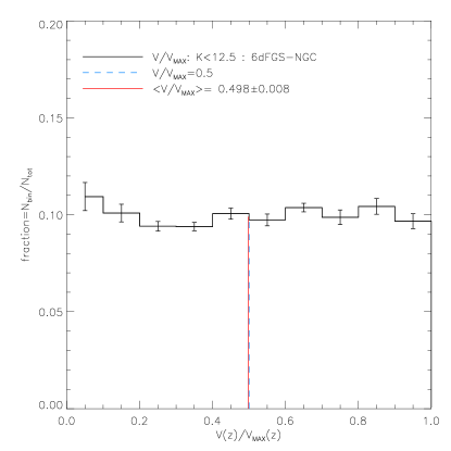
Figure 1: A histogram of K band galaxy $V/V_{max}$ with $7.5<K<12.5$ for the 6dFGS-NGC data with corresponding jackknife error. The (blue, dashed) line shows the homogeneous expectation that $\langle V/V_{max}\rangle=0.5$. Also shown is the mean $\langle V/V_{max}\rangle$ for 6dFGS-NGC data (red, solid line).

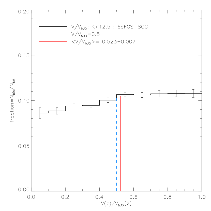
Figure 2: A histogram of K band galaxy $V/V_{max}$ with $7.5<K<12.5$ for the 6dFGS-SGC data with corresponding jackknife error. The (blue, dashed) line shows the homogeneous, expectation that $\langle V/V_{max}\rangle=0.5$. Also shown is the mean $\langle V/V_{max}\rangle$ for 6dFGS-SGC data (red, solid line).

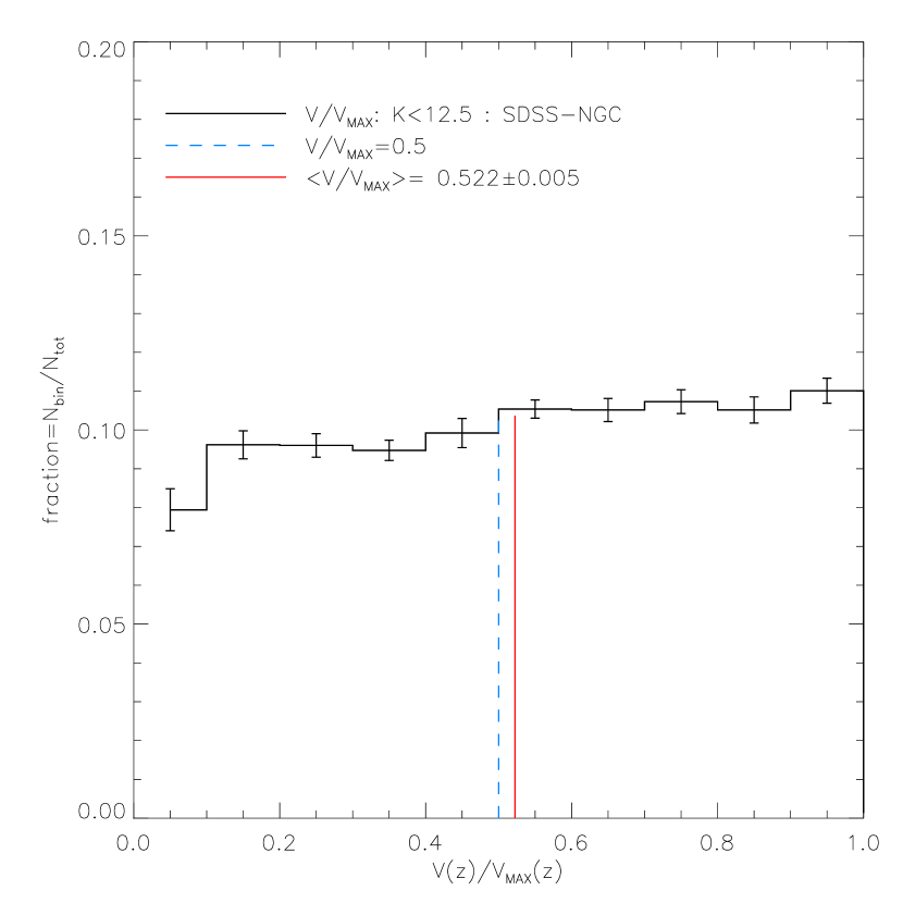
Figure 3: A histogram of K band galaxy $V/V_{max}$ with $7.5<K<12.5$ for the SDSS-NGC data with corresponding jackknife error. The (blue, dashed) line shows the homogeneous expectation that $\langle V/V_{max}\rangle=0.5$. Also shown is the mean $\langle V/V_{max}\rangle$ for SDSS-NGC data (red, solid line).

4.2 K band LF estimates

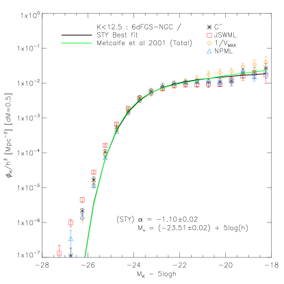
Figure 4: K band galaxy LF estimates with $7.5<K<12.5$ and d$M=0.5$ for the 6dFGS-NGC data. All of the estimates have been normalised using the $n_{1}$ number density estimator for their respective LF.

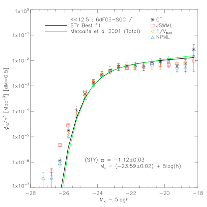
Figure 5: K band galaxy LF estimates with $7.5<K<12.5$ and d$M=0.5$ for the 6dFGS-SGC data. All of the estimates have been normalised using the $n_{1}$ number density estimator for their respective LF.

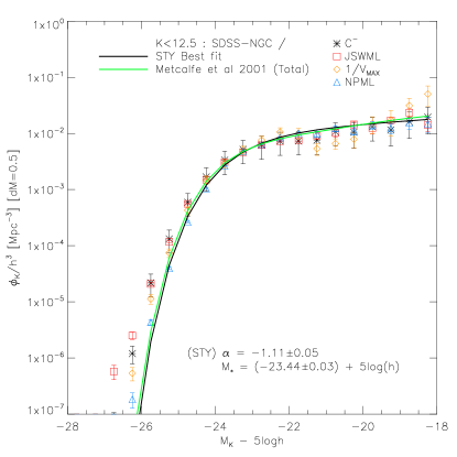
Figure 6: K band galaxy LF estimates with $7.5<K<12.5$ and d$M=0.5$ for the SDSS-NGC data. All of the estimates have been normalised using the $n_{1}$ number density estimator for their respective LF.

We next use the LF estimators described in Sec. 2 to estimate the K band LF in our three regions. In Figs 4-6 we show these estimates for the 6dFGS-NGC, 6dFGS-SGC and SDSS-NGC regions, respectively. These LF’s have been normalised using their respective estimate of $n_{1}$.

Treating these fields in turn, we begin with the 6dFGS-NGC field shown in Fig. 4. We first note that the LF estimators are in agreement with the Metcalfe et al. (2001, 2006) type dependent Schechter LF (green solid line) until the very bright end ($<M_{*}-2$). The Metcalfe et al LF is an optical LF which is translated into the NIR using an assumed mean colour so this agreement was not to be taken for granted. We also note that the parametric Schechter function fits provided by the STY method is in agreement with the other non-parametric LF estimates over much of the range in absolute magnitude. However, for the very bright end ($<M_{*}-2$) the STY result is an underestimate with respect to the nonparametric estimates. We interpret this as suggesting that Schechter parametrisation of the LF is accurate in the main but does not fully represent the abundance of very bright objects such as brightest cluster galaxies - a conclusion also reached by other authors (Jones et al., 2006).

For the 6dFGS-SGC region shown in Fig. 5 we see a similar set of estimates to those obtained in the 6dFGS-NGC region up until the faint end ($<M_{*}+2$). The Metcalfe et al LF is a reasonable fit to all the estimators over all but the brightest and faintest magnitudes. Indeed, this time the parametric estimator, the STY method, agrees well with the non-parametric estimates except for $<M_{*}-2$ and $<M_{*}+2$. We again assign this relative excess of faint objects and deficit of bright objects relative to the nonparametric fits as due to a limitation of this parametrisation. We also note that the $V_{max}$ estimator is significantly different from the other estimates. We attribute this to the inhomogeneity reported in this field in Paper I. This is consistent with the elevated value of $\langle V/V_{max}\rangle=(0.523\pm 0.007)$ in this region as discussed in Sec. 4.

Now in Fig. 6 we show the LF estimators for SDSS-NGC region. We draw similar conclusions to the previous 6dFGS-SGC region. In particular the $V/V_{max}$ LF estimate is again significantly different from the other estimators, especially at the faint end. We again attribute this to a significant inhomogeneity as indicated in this field by the elevated value of $\langle V/V_{max}\rangle=(0.522\pm 0.005)$ discussed in Sec. 4. We note that the bright end excess relative to the Schechter parametric fits is less pronounced in this field. We also observe that whilst the STY $\alpha$ estimates are mutually consistent between the fields the differences in the $M_{*}$ estimates, although small, are significant. But in any case the differences are relatively minor in the sense that the Metcalfe et al LF is a good representation of all the LF estimators except at the bright end.

We therefore conclude that the Metcalfe et al LF is a adequate fit to the majority of the K band LF estimators in all three fields. We take this as providing evidence supporting our assumption of the Metcalfe et al LF in Paper I - and hence the density profiles we then estimated using number counts. However, we can now continue this investigation beyond the LF and make use of the density profiles and normalisation information provided by the various LF estimates to study the homogeneity of our samples.

5 K band normalised number density profiles

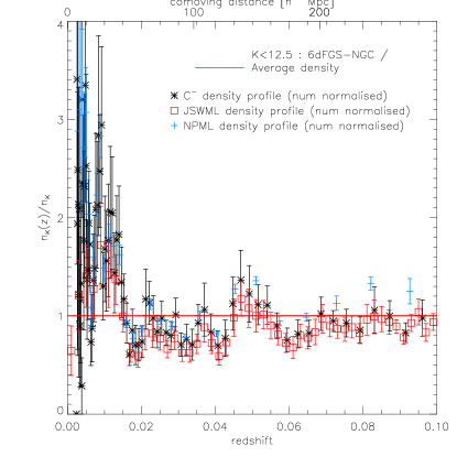
Figure 7: K band galaxy number underdensity profile with $7.5<K<12.5$ for the 6dFGS-NGC data normalised (for each LF) to the number counts in the region. The red (solid) line represents the homogeneous prediction for each LF.

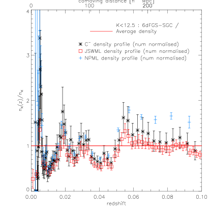
Figure 8: K band galaxy number underdensity profile with $7.5<K<12.5$ for the 6dFGS-SGC data normalised (for each LF) to the number counts in the region. The red (solid) line represents the homogeneous prediction for each LF.

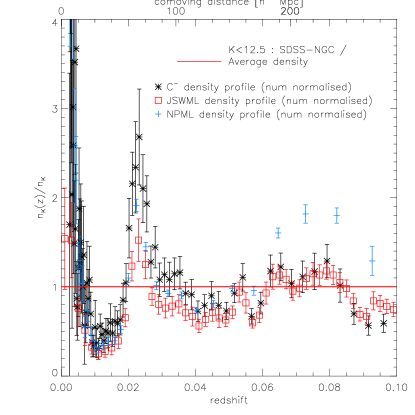
Figure 9: K band galaxy number underdensity profile with $7.5<K<12.5$ for the SDSS-NGC data normalised (for each LF) to the number counts in the region. The red (solid) line represents the homogeneous prediction for each LF.

As outlined in Sec. 2 we can use the NPML, JSWML and $C^{-}$ methods to estimate the run of the number density profile. The normalisations used are dependent on the estimator. The profiles presented here have been normalised using their respective LF based number counts. Similar results, at greater uncertainty, are found when using the $n_{1}$ unbiased number density estimator (i.e. equation 12) calculated using the corresponding LF. We now present in Figs 7-9 these number density profiles for the 6dFGS-NGC, 6dFGS-SGC and SDSS-NGC regions, respectively.

For the 6dFGS-NGC region (Fig. 7) we observe good consistency between the various estimates of the number density run. We can also see the inhomogeneity inferred from this field’s $V/V_{max}$ statistic in that locally ($z<0.05$) the profiles are typically underdense and then transition to being reasonably homogeneous. We also observe significant LSS clustering with significant fluctuations in the density profile at $z\approx 0.048$ which we attribute to the Shapley-8 supercluster. We also note that this profile is similar to that presented in Paper I (fig. 3a) for the 6dFGS-NGC field where the Metcalfe et al LF was assumed. This is inline with the agreement we noted in Sec. 4.2 between the Metcalfe et al. LF and the LF estimates we have made here.

In Fig. 8 we show the number density profile for the 6dFGS-SGC field. We again see good agreement between the different estimators of the density profile. However, at high redshift ($z>0.05$) the NPML estimate is significantly higher than the JSWML and $C^{-}$ estimates. This is true for all three K-band fields and may therefore be indicative of a lack of robustness at high redshift for the NPML estimate. All profile estimates are particularly underdense at local redshift with the JSWML and $C^{-}$ becoming homogeneous at deeper redshifts. We again note the agreement with the Paper I (fig. 3b) number density profile for this field which once more reflects the validity of the Metcalfe et al LF for the sample in this field.

Finally, in Fig. 9 we show the number density profile for the SDSS-NGC region. Here we see a similar pattern of agreement between the different number density profiles. The JSWML, NPML and $C^{-}$ profiles are in agreement at low redshift in showing an underdense profiles with significant LSS (which we attribute to Coma at $z=0.023$). At deeper redshifts ($z>0.08$), the density profiles show evidence of an extensive overdensity. We return to investigate this issue using the deeper r band data over the same field. However, we also note that this substantially inhomogeneous profile is in agreement with the density profile estimated in Paper I (fig. 3c).

We have evaluated the corresponding number under-density indicated by these profiles as

$$\frac{\int_{0}^{z_{1}}\frac{n(z)}{n_{K}}\frac{dV}{dz}.dz}{\int_{0}^{z_{1}}dV}$$ (13)

The average of the profile number underdensities are reported in Table 1 for $z<0.05$, i.e. $\approx 150$h^-1Mpc, and $z<0.1$, i.e. $\approx 300$h^-1Mpc in the 6dFGS-NGC, 6dFGS-SGC and SDSS-NGC regions. Errors have been inferred using jackknife estimates. We noted earlier the potential lack of robustness at high redshift for the NPML estimator. We have therefore disregarded the NPML profiles in calculating the $z<0.1$ average underdensities.

These results are broadly consistent with the underdensities reported in Paper I (table 4) - aside from the 6dFGS-SGC estimate. In this case, both the $z<0.05$ (now $0.76\pm 0.05$, previously $0.60\pm 0.05$) and $z<0.1$ results (now $1.02\pm 0.11$, previously $0.75\pm 0.04$) are less underdense. Indeed the $z<0.1$ result is now consistent with homogeneity, albeit with larger errors. However, this difference is relatively minor in that the results presented here based on number count normalised number density profiles are in agreement with the 6dFGS-SGC number count underdensity reported in Paper I ($0.76\pm 0.03$).

We therefore conclude that the density profiles show evidence for an LSS local underdensity for $z<0.05$ which the SDSS-NGC field in particular suggests may extend to deeper depths ($\approx 300$h^-1Mpc). These conclusions are in agreement with those presented in Paper I which reflects the agreement found here with the Metcalfe et al LF used in that study.

Field	Sample limit	Under-density
6dFGS-NGC	$z<0.05$	$0.95\pm 0.11$
6dFGS-SGC	$z<0.05$	$0.76\pm 0.05$
SDSS-NGC	$z<0.05$	$0.83\pm 0.05$
6dFGS-NGC	$z<0.1$	$0.91\pm 0.08$
6dFGS-SGC	$z<0.1$	$1.02\pm 0.11$
SDSS-NGC	$z<0.1$	$0.89\pm 0.06$

Table 1: A summary of the average underdensities derived using eqn. (13). The $z<0.05$ and $z<0.1$ entries use $7.5<K<12.5$.

6 ${r}\leq 17$ LF and density profiles in the SDSS-NGC region

Using the SDSS survey it is possible to go to deeper survey limits than in the K-band. In particular, following Paper I, we use an r band limited sample in order to investigate the SDSS-NGC field. We have used a more conservative r-band magnitude limit of $r\leq 17$ than the $r\leq 17.2$ limit used in Paper I in order to minimise any potential biasing/issues associated with spectroscopic incompleteness.

Now in Fig. 10 we show the $V/V_{max}$ estimates. We report a mean value of $(0.500\pm 0.003)$. This value is consistent with the homogeneous expectation and indeed the uniformity in this statistic shows little evidence for an underdensity. This is significantly different from the slope observed in Fig. 3 where the K band SDSS-NGC $V/V_{max}$ estimates are shown. A similar and related situation was encountered in Paper I when comparing the results r and K band counts over the same field. Here it was concluded that the evidence for an underdensity in the r band was more ambiguous and more suggestive of $150h^{-1}$ scale underdensity which was punctuated by the strong clustering associated with the Coma supercluster. This is potentially consistent with the broader smoothing effect of the d$(V/V_{max})=0.1$ binning used for the deeper r band sample which may smooth over local variations in the density profile. We therefore proceed to investigate r-band LF’s and the resulting density profiles.

In Fig. 11 we show the LF estimates for the SDSS-NGC region r band data. We see that there is good agreement between the variety of LF estimates except for the very brightest objects ($<M_{*}-3$). We also note that the $C^{-}$ estimator has a shallower faint end slope than compared to our other LF estimators. However, again, these differences are relatively minor in that the Metcalfe et al LF is a good representation of our results over a wide range of magnitudes.

We therefore show in Fig. 12 the density profiles associated with JSWML, $C^{-}$ and NPML LF estimates r-band SDSS-NGC density profiles. The JSWML, $C^{-}$ and NPML profiles are in good agreement in showing underdense profiles with significant LSS (which we attribute to Coma at $z=0.023$). At deeper redshifts ($z>0.08$) the $C^{-}$, NPML and JSWML density profiles remain significantly inhomogeneous. This is consistent with the investigation of fainter GAMA K band and SDSS r band $n(m)$ and $n(z)$ in Paper I which indicated that an inhomogeneity could extend beyond $z=0.1$ in the SDSS-NGC region. We also note that the r-band density profiles demonstrate a similar local underdensity ($z<0.08$) to that seen over the same field in the K band (see Fig. 9).

Finally, we have evaluated the average number underdensity following equation (13) with the results shown in Table 2. We now include the NPML density profiles for the $z<0.1$ results as there is no evidence of lack of robustness at high redshift for the r band sample. For $z<0.05$ we find an average number underdensity of $[0.83\pm 0.05]$ which is in agreement with the K band SDSS-NGC results in suggesting a significant local number underdensity ($\approx 150$h^-1Mpc). Whilst the $z<0.1$ average number underdensity of $[0.90\pm 0.03]$ indicates a more extensive inhomogeneity on $\approx 300$h^-1Mpc scales. Both these results are in agreement with the results presented in Paper I.

We conclude that the r-band density profiles show evidence for an underdensity, which is punctuated by the Coma cluster producing a strong overdensity. This underdensity is similar to those observed for the corresponding region in the K band (Fig. 9) but less than that observed in the K band over the SGC (Fig. 8).

Figure 10: A histogram of r band galaxy $V/V_{max}$ with $10<r<17$ for the SDSS-NGC data with a corresponding jackknife error. The (blue, dashed) line shows the homogeneous, complete expectation that $\langle V/V_{max}\rangle=0.5$. Also shown is the mean $\langle V/V_{max}\rangle$ for SDSS-NGC data (red, solid line).

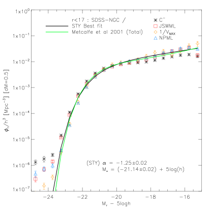
Figure 11: r band galaxy LF estimates with $10<r<17$ and d$M=0.5$ for the SDSS-NGC data. All of the estimates have been normalised using the $n_{1}$ number density estimator for their respective LF.

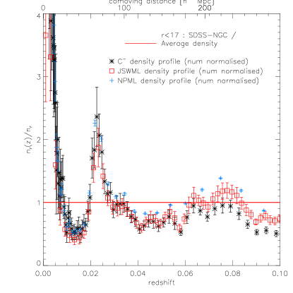
Figure 12: r band galaxy number density profile with $10<r<17$ for the SDSS-NGC data normalised (for each LF) to the number counts in the region. The red (solid) line represents the homogeneous prediction for each LF.

Field	Sample limit	Under-density
SDSS-NGC	$z<0.05$	$0.83\pm 0.05$
SDSS-NGC	$z<0.10$	$0.90\pm 0.03$

Table 2: A summary of the average underdensities derived using eqn. (13). The $z<0.05$ and $z<0.1$ entries use $10<r<17$.

7 Discussion

We note that any estimation of the LF is strongly dependent on accurate and stable galaxy photometry. Paper I includes a fuller discussion of the photometric completeness of these samples. However, we have estimated the effect of magnitude errors on our NIR LF estimation using the method of Efstathiou, Ellis & Peterson (1988) where the observed LF is described as the convolution of the true underlying LF with a magnitude error kernel, i.e. $\phi_{obs}(M)=g(M)\otimes\phi_{true}(M)$. Using realistic magnitude error kernels derived from fig. A1 of Paper I we find that the effects of magnitude errors on the K-band LF typically steepen the faint end slope by $\approx 0.1$ and similarly brighten the characteristic magnitude by $\approx 0.1$. We have investigated the uncertainty this corresponds to in our determination of the galaxy number density profiles by testing the variation induced in the Cole (2011) density profiles if a realistic magnitude error is allowed. We found that the changes were small, typically $<1-2\%$ (K and r band respectively) and random in nature. It should be noted that larger ($\approx 5\%$) variations were possible for low and high z ($z<0.01$ and $z>0.1$). However, over the redshift range of interest we conclude that magnitude errors only weakly affect our density profile estimates.

We again follow Paper I in the treatment of completeness issues. We note that the inclusion of corrections for incompleteness detailed for the $V_{max}$, $C^{-}$ and STY methods are relatively minor in determining the LF or number density profiles. Finally, we also again note that we have used the $vc$ 2MASS quality flag to reject artifact and non-extragalactic objects. This ensures that $\approx$100% of objects $7.5<K<12.5$ have been visually inspected to ensure a high purity sample.

An important assumption in this work has been the use of the $K+E$ prescriptions used in Metcalfe et al. (2001, 2006). In order to explain the observed underdensity we would require evolutionary brightening at $z\approx 0.1$ or a more negative K-correction. As was noted in Paper I an argument against the rise in number density being caused by $z\approx 0.1$ galaxy evolution is the rise in number counts across the NIR and optical bands (B,R,I,H,K) Metcalfe et al. (2001, 2006). A local underdensity produces just this, an approximately band-independent rise in the bright number counts whereas evolutionary effects correspond to a greater effect in the bluer bands and at fainter magnitudes. We also note that in Paper I we investigated alternative evolutionary models as well as no evolutionary corrections and found minimal differences in the K-band (although not for the r-band) in terms of derived redshift distributions and number counts.

The three fields studied here are wide field, with each representing $\approx 1/15$ of the sky. However, they are considerably smaller than the full sky 2MASS sample from which they are drawn. We note however that Appleby & Shafieloo (2014) have investigated the isotropy of LF shape estimates using the 2MPZ, a set of photometric redshifts estimated in Bilicki et al. (2014) for the 2MASS-XSC sample. These authors find no significant evidence for anisotropy in non-parametric LF shape estimates. This suggests that the three fields used in this study should be representative of the full 2MASS survey. It should be noted that the LF normalisation was not investigated in this paper so this result is not in tension with the varying galaxy number density profiles presented in this study. Furthermore, it is also of interest that these authors report weak evidence for a dipole asymmetry in parametric LF estimates between the north and south galactic plane. This is again in agreement with the significantly different density profiles found for the 6DFGS-SGC, 6DFGS-NGC and SDSS-NGC regions.

Other estimates of the NIR LF using these samples have been attempted. We therefore now present in Figs 14 & 14 a comparison to other studies estimates of the Schechter $\alpha$ and $M_{*}$ parameters. In Fig. 14 we show a comparison of the full $\phi(M)$ because it captures the correlation between the $\alpha$ and $M_{*}$ parameters. We also include in this comparison our JSWML non parametric LF estimates (SDSS-NGC) so that any deviations from the Schechter form can be judged. After normalising to a common and arbitrary number density [estimated using the Metcalfe et al LF over the range $-28\leq M-5\log(h)\leq-18$] we find that the K-band LF estimates are relatively consistent, except at the faint end where there is greater variance. In particular, the Metcalfe et al LF shows a much steeper faint-end slope than found by Bell et al. (2003) using the $V_{max}$ estimator with the 2MASS survey. We attribute this to photometric problems in the early 2MASS data releases since in the same work the g-band selected NIR LF was estimated to have a faint end slope of $\alpha=-1.33$ which is in rough agreement with the steeper slope of the Metcalfe et al LF.

In Fig. 14 most K-band LF parameterisations occupy the usual degenerate strip between $M^{*}$ and $\alpha$. The one that most deviates from this line is the LF of Jones et al. (2006) (see also Fig.14). We also note that the variation between different LF estimates is much larger than would be expected on the basis of the ‘naive’ error ellipses (i.e. the no covariance case). We do not understand what causes these differences but potential causes of differences are different treatment of flow models, incompleteness, as well as real differences in sample selection (magnitude limits, redshift ranges, etc.).

We have made a similar comparison for r band LF estimates in Figs 16 & 16. We have again normalised to an arbitrary number density estimated using the Metcalfe et al LF over the range $-25\leq M-5\log(h)\leq-15$. Results quoted in the $r_{0.1}$ band (i.e. corrected to a $z=0.1$ rest frame as per Blanton et al. 2003) have been converted into the $r$ band as $r_{0.1}\approx r+0.23$ (Nichol et al., 2006). We find results that are consistent with the Metcalfe et al LF. However, the Blanton et al. (2003) and Driver et al. (2012) estimates show a significantly sharper bright end fall off and a shallower faint end slope than the Metcalfe et al LF. The greater uncertainties in the assumed evolutionary model for the r-band as compared to the K may explain the difference with the Driver et al. (2012) LF since the GAMA survey probes a substantially deeper redshift range than the samples used in this paper. However, this is an unlikely explanation for the difference with the SDSS based Blanton et al. (2003) LF, especially as any evolutionary modelling effects would be expected to primarily affect $M_{*}$ estimates. It is therefore unclear why these results are different from those presented here. However, we agree with the observation of Montero-Dorta & Prada (2009) that the size of the SDSS sample has increased considerably since the pre SDSS-DR1 results used in Blanton et al. (2003). The resulting improvements in magnitude limits may have resulted in substantial improvements in sample selection. The potential uncertainty that differences in the LF correspond to in the number density profiles is indicated by the differences between the $C^{-}$, JSWML and NPML density profiles in Fig. 12. This is particularly relevant in the case of the $C^{-}$ LF estimate where we find a flatter faint end slope than the JSWML or NPML estimates (see Fig. 11) but nevertheless find similar number density profiles.

Again many, r-band LF parameterisations occupy the usual degenerate strip between $M^{*}$ and $\alpha$ in Fig. 16. The two that most deviate from this line are the LF’s of Loveday et al. (2012) and Montero-Dorta & Prada (2009) (see also Fig.16). However, this small deviation may be attributable to the correction applied to convert from the $r_{0.1}$ and r bands. Fig. 16 also confirms the much flatter parametric faint end slope reported by Blanton et al. (2003) than seen by later authors, including ourselves.

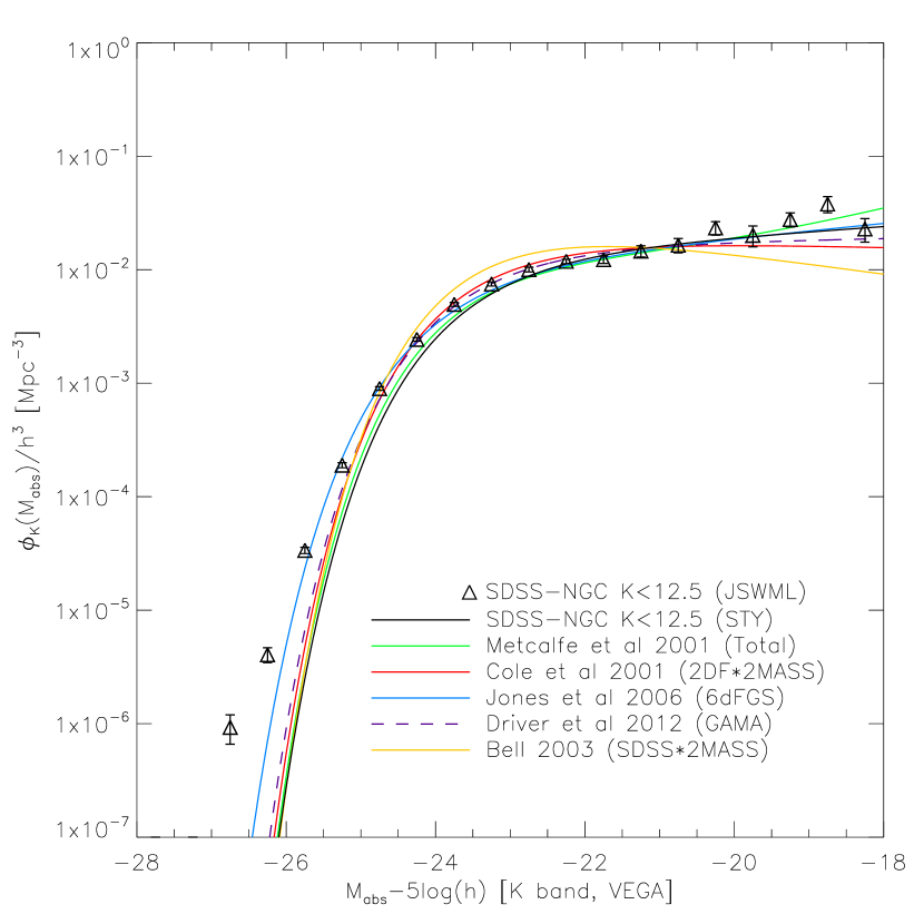
Figure 13: A comparison of various parametric K band LF estimates using the full $\phi_{K}(M)$. Results have been normalised to a common and arbitrary number density estimated using the Metcalfe et al LF over the range $-28\leq M-5\log(h)\leq-18$. Parameters taken from Cole et al. (2001), Jones et al. (2006), Driver et al. (2012) and Bell et al. (2003).

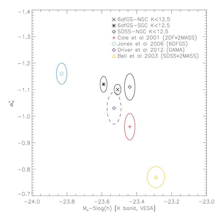
Figure 14: A comparison of various K band parametric LF estimates of the Schechter $\alpha$ and $M_{*}$ parameters. We have not been able to represent the covariance between $\alpha$ and $M_{*}$ from the studies shown so we assume no covariance.

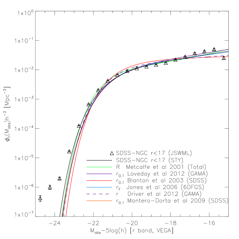
Figure 15: A comparison of various r band LF estimates using the full $\phi_{r}(M)$. Results have been normalised to a common and arbitrary number density estimated using the Metcalfe et al LF over the range $-25\leq M-5\log(h)\leq-15$. Parameters taken from Loveday et al. (2012), Jones et al. (2006), Blanton et al. (2003), Driver et al. (2012) and Montero-Dorta & Prada (2009). Results quoted in the $r_{0.1}$ band have been converted into the $r$ band as $r_{0.1}\approx r+0.23$ (Nichol et al., 2006).

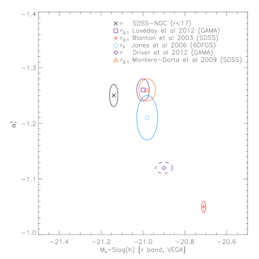
Figure 16: A comparison of various r band parametric LF estimates of the Schechter $\alpha$ and $M_{*}$ parameters. We have not been able to represent the covariance between $\alpha$ and $M_{*}$ from the studies shown so we assume no covariance. Again, results quoted in the $r_{0.1}$ band have been converted into the $r$ band as $r_{0.1}\approx r+0.23$ (Nichol et al., 2006)

8 Conclusions

We have used samples from 6dFGS/2MASS and SDSS to simultaneously investigate the local LF and galaxy number density profiles. We have studied three large volumes which cover much of the sky and find evidence for an anisotropic galaxy distribution. In particular we observe a local number underdensity out to $\approx 150$h^-1Mpc around our position in the SGC which both the r and K band SDSS-NGC samples suggest may extend deeper to $\approx 300$h^-1Mpc. We have also found evidence that the Metcalfe et al LF assumed in Paper I is an adequate fit for these samples and hence the density profiles presented there may be unbiased by this choice. This work also complements previous studies which have investigated variation of luminosity density with redshift (Keenan et al., 2012; Keenan, Barger & Cowie, 2013) by providing estimates of variation in number density. The estimate made in Paper I of an $\approx 15\%$ number underdensity is broadly consistent with the Keenan, Barger & Cowie (2013) estimate of an $\approx 50\%$ increase in luminosity between the local universe and $z\approx 0.1$.

A significant advantage of investigating both the K and r bands is that an underdensity might be indicated if the effect is band independent, although a band-dependent result might still be explained by different galaxy clustering bias applying in the different bands. We note that the r-band SDSS-NGC profile (Fig. 12) shows a similar underdensity to the corresponding K-band estimate (Fig. 9) with only small differences at low redshift. But both are in agreement in supporting an underdensity continuing beyond $z\approx 0.1$. One important route for continuing the investigation into the isotropy of the galaxy distribution will be the incorporation of peculiar velocity fields. We therefore believe that the ongoing investigation into the 6DFGS peculiar velocity field as determined using the Fundamental Plane (and its comparison to that inferred from PSCz) started in Springob et al. (2014) will be of particular interest. We note that the initial analysis presented in Springob et al. (2014) is in agreement with the PSCz estimated density field (to a separately estimated 2MRS peculiar velocity field based on an update of Erdoğdu et al. 2006) which has a mean underdensity of $11\%$ within $180h^{-1}$Mpc. The density profiles presented here are consistent with such a local underdensity.

Acknowledegments

We thank Richard Fong, John Lucey, Alan Heavens and Ryan Keenan for useful comments. JRW acknowledges financial support from STFC. We would also like to thank the anonymous referee for their comments.

We acknowledge the use of a modified version of the JSWML code accompanying Cole (2011).

This research has made use of the NASA/IPAC Extragalactic Database (NED) which is operated by the Jet Propulsion Laboratory, California Institute of Technology, under contract with the National Aeronautics and Space Administration.

We would also like to acknowledge the use of the TOPCAT utility (Taylor, 2005).

This research has made use of the VizieR catalogue access tool, CDS, Strasbourg, France”. The original description of the VizieR service was published in A&AS 143, 23 (2000).

Funding for the SDSS and SDSS-II has been provided by the Alfred P. Sloan Foundation, the Participating Institutions, the National Science Foundation, the U.S. Department of Energy, the National Aeronautics and Space Administration, the Japanese Monbukagakusho, the Max Planck Society, and the Higher Education Funding Council for England. The SDSS Web Site is http://www.sdss.org/.

The SDSS is managed by the Astrophysical Research Consortium for the Participating Institutions. The Participating Institutions are the American Museum of Natural History, Astrophysical Institute Potsdam, University of Basel, University of Cambridge, Case Western Reserve University, University of Chicago, Drexel University, Fermilab, the Institute for Advanced Study, the Japan Participation Group, Johns Hopkins University, the Joint Institute for Nuclear Astrophysics, the Kavli Institute for Particle Astrophysics and Cosmology, the Korean Scientist Group, the Chinese Academy of Sciences (LAMOST), Los Alamos National Laboratory, the Max-Planck-Institute for Astronomy (MPIA), the Max-Planck-Institute for Astrophysics (MPA), New Mexico State University, Ohio State University, University of Pittsburgh, University of Portsmouth, Princeton University, the United States Naval Observatory, and the University of Washington.

This publication makes use of data products from the Two Micron All Sky Survey, which is a joint project of the University of Massachusetts and the Infrared Processing and Analysis Center/California Institute of Technology, funded by the National Aeronautics and Space Administration and the National Science Foundation.

References

- Appleby & Shafieloo (2014) Appleby S., Shafieloo A., 2014, J. Cosmology Astropart. Phys., 10, 70
- Bell et al. (2003) Bell E. F., McIntosh D. H., Katz N., Weinberg M. D., 2003, ApJS, 149, 289
- Bilicki et al. (2014) Bilicki M., Jarrett T. H., Peacock J. A., Cluver M. E., Steward L., 2014, ApJS, 210, 9
- Blanton et al. (2003) Blanton M. R., Hogg D. W., Bahcall N. A., et al., 2003, ApJ, 592, 819
- Böhringer et al. (2015) Böhringer H., Chon G., Bristow M., Collins C. A., 2015, A&A, 574, A26
- Bruzual & Charlot (2003) Bruzual G., Charlot S., 2003, MNRAS, 344, 1000
- Busswell et al. (2004) Busswell G. S., Shanks T., Frith W. J., Outram P. J., Metcalfe N., Fong R., 2004, MNRAS, 354, 991
- Carroll (2001) Carroll S. M., 2001, Living Reviews in Relativity, 4, 1
- Choloniewski (1986) Choloniewski J., 1986, MNRAS, 223, 1
- Choloniewski (1987) Choloniewski J., 1987, MNRAS, 226, 273
- Clarkson & Maartens (2010) Clarkson C., Maartens R., 2010, Classical and Quantum Gravity, 27, 124008
- Cole (2011) Cole S., 2011, MNRAS, 416, 739
- Cole et al. (2001) Cole S., Norberg P., Baugh C. M., et al., 2001, MNRAS, 326, 255
- Colin et al. (2011) Colin J., Mohayaee R., Sarkar S., Shafieloo A., 2011, MNRAS, 414, 264
- Conley et al. (2007) Conley A., Carlberg R. G., Guy J., Howell D. A., Jha S., Riess A. G., Sullivan M., 2007, ApJL, 664, L13
- Davis & Huchra (1982) Davis M., Huchra J., 1982, ApJ, 254, 437
- de Lapparent, Geller & Huchra (1989) de Lapparent V., Geller M. J., Huchra J. P., 1989, ApJ, 343, 1
- Driver et al. (2012) Driver S. P., Robotham A. S. G., Kelvin L., et al., 2012, MNRAS, 427, 3244
- Efstathiou, Ellis & Peterson (1988) Efstathiou G., Ellis R. S., Peterson B. A., 1988, MNRAS, 232, 431
- Erdoğdu et al. (2006) Erdoğdu P. et al., 2006, MNRAS, 373, 45
- Feindt et al. (2013) Feindt U., Kerschhaggl M., Kowalski M., Aldering G., et al., 2013, A&A, 560, A90
- Felten (1976) Felten J. E., 1976, ApJ, 207, 700
- Frith et al. (2003) Frith W. J., Busswell G. S., Fong R., Metcalfe N., Shanks T., 2003, MNRAS, 345, 1049
- Frith, Outram & Shanks (2005) Frith W. J., Outram P. J., Shanks T., 2005, in Astronomical Society of the Pacific Conference Series, Vol. 329, Nearby Large-Scale Structures and the Zone of Avoidance, A. P. Fairall & P. A. Woudt, ed., pp. 49–+
- Frith, Outram & Shanks (2006) Frith W. J., Outram P. J., Shanks T., 2006, MNRAS, 373, 759
- Frith, Shanks & Outram (2005) Frith W. J., Shanks T., Outram P. J., 2005, MNRAS, 361, 701
- Ilbert et al. (2005) Ilbert O., Tresse L., Zucca E., et al., 2005, A&A, 439, 863
- Jarrett et al. (2003) Jarrett T. H., Chester T., Cutri R., Schneider S. E., Huchra J. P., 2003, AJ, 125, 525
- Jha, Riess & Kirshner (2007) Jha S., Riess A. G., Kirshner R. P., 2007, ApJ, 659, 122
- Johnston (2011) Johnston R., 2011, A&A Rev., 19, 41
- Jones et al. (2006) Jones D. H., Peterson B. A., Colless M., Saunders W., 2006, MNRAS, 369, 25
- Jones et al. (2004) Jones D. H., Saunders W., Colless M., Read M. A., et al., 2004, MNRAS, 355, 747
- Kafka (1967) Kafka P., 1967, Nature, 213, 346
- Keenan, Barger & Cowie (2013) Keenan R. C., Barger A. J., Cowie L. L., 2013, ApJ, 775, 62
- Keenan et al. (2012) Keenan R. C., Barger A. J., Cowie L. L., Wang W.-H., Wold I., Trouille L., 2012, ApJ, 754, 131
- Keenan et al. (2010) Keenan R. C., Trouille L., Barger A. J., Cowie L. L., Wang W., 2010, ApJS, 186, 94
- Krasiński (2014) Krasiński A., 2014, PhRvD, 89, 023520
- Loveday et al. (2012) Loveday J., Norberg P., Baldry I. K., et al., 2012, MNRAS, 420, 1239
- Lynden-Bell (1971) Lynden-Bell D., 1971, MNRAS, 155, 95
- Metcalfe et al. (2001) Metcalfe N., Shanks T., Campos A., McCracken H. J., Fong R., 2001, MNRAS, 323, 795
- Metcalfe et al. (2006) Metcalfe N., Shanks T., Weilbacher P. M., McCracken H. J., Fong R., Thompson D., 2006, MNRAS, 370, 1257
- Montero-Dorta & Prada (2009) Montero-Dorta A. D., Prada F., 2009, MNRAS, 399, 1106
- Nichol et al. (2006) Nichol R. C. et al., 2006, MNRAS, 368, 1507
- Perlmutter et al. (1999) Perlmutter S., Aldering G., Goldhaber G., et al., 1999, ApJ, 517, 565
- Planck Collaboration et al. (2014) Planck Collaboration et al., 2014, A&A, 571, A16
- Sandage, Tammann & Yahil (1979) Sandage A., Tammann G. A., Yahil A., 1979, ApJ, 232, 352
- Schechter (1976) Schechter P., 1976, ApJ, 203, 297
- Schmidt et al. (1998) Schmidt B. P., Suntzeff N. B., Phillips M. M., et al., 1998, ApJ, 507, 46
- Schmidt (1968) Schmidt M., 1968, ApJ, 151, 393
- Schwarz (2012) Schwarz D. J., 2012, Cosmological backreaction, The Twelfth Marcel Grossmann Meeting, pp. 563–577
- Shanks (1990) Shanks T., 1990, in IAU Symposium, Vol. 139, The Galactic and Extragalactic Background Radiation, Bowyer S., Leinert C., eds., pp. 269–281
- Soneira (1979) Soneira R. M., 1979, ApJL, 230, L63
- Springob et al. (2014) Springob C. M. et al., 2014, MNRAS, 445, 2677
- Takeuchi, Yoshikawa & Ishii (2000) Takeuchi T. T., Yoshikawa K., Ishii T. T., 2000, ApJS, 129, 1
- Taylor (2005) Taylor M. B., 2005, in Astronomical Society of the Pacific Conference Series, Vol. 347, Astronomical Data Analysis Software and Systems XIV, Shopbell P., Britton M., Ebert R., eds., p. 29
- Whitbourn & Shanks (2014) Whitbourn J. R., Shanks T., 2014, MNRAS, 437, 2146
- Willmer (1997) Willmer C. N. A., 1997, AJ, 114, 898
- Wojtak et al. (2014) Wojtak R., Knebe A., Watson W. A., Iliev I. T., Heß S., Rapetti D., Yepes G., Gottlöber S., 2014, MNRAS, 438, 1805
- York et al. (2000) York D. G., Adelman J., Anderson, Jr. J. E., et al., 2000, AJ, 120, 1579
- Zehavi et al. (1998) Zehavi I., Riess A. G., Kirshner R. P., Dekel A., 1998, ApJ, 503, 483
- Zucca, Pozzetti & Zamorani (1994) Zucca E., Pozzetti L., Zamorani G., 1994, MNRAS, 269, 953
- Zucca et al. (1997) Zucca E., Zamorani G., Vettolani G., et al., 1997, A&A, 326, 477