Fluids confined in wedges and by edges:
virial series for the line-thermodynamic properties of hard spheres

Abstract

This work is devoted to analyze the relation between the thermodynamic properties of a confined fluid and the shape of its confining vessel. Recently, new insights in this topic were found through the study of cluster integrals for inhomogeneous fluids, that revealed the dependence on the vessel shape of the low density behavior of the system. Here, the statistical mechanics and thermodynamics of fluids confined in wedges or by edges is revisited, focusing on their cluster integrals. In particular, the well known hard sphere fluid, which was not studied in this framework so far, is analyzed under confinement and its thermodynamic properties are analytically studied up to order two in the density. Furthermore, the analysis is extended to the confinement produced by a corrugated wall. These results rely on the obtained analytic expression for the second cluster integral of the confined hard sphere system as a function of the opening dihedral angle $0<\beta<2\pi$. It enables a unified approach to both wedges and edges.

I Introduction

The thermodynamic properties of fluids are influenced by the geometry of either the vessel or substrate, which constrain the spatial region where the molecules of the systems move. Several efforts are continuously devoted to reach a detailed description of the response of fluids to some of the simplest geometrical constraints, including the confinement in pores with slit, cylindrical and spherical shapes, as well as the case of fluids in contact with planar and curved walls. Even more, the behavior of fluids adsorbed in wedges, at edges,Henderson (2002, 2004a, 2004b); Boţan et al. (2009) and geometrically structured surfaces was the subject of several studies during the last decade.Schneemilch, Quirke, and Henderson (2003); Bryk et al. (2003); Schoen (2002) The interest on confined inhomogeneous fluids covers a wide range of complexity and particles size, which starts at the simplest one-atom per molecule (e.g. the noble gases) and goes up to proteins, polymers (including DNA molecules) and large colloids.Henderson (2006); Almenar and Rauscher (2011); Freed and Wu (2011); Lutsko (2012); Statt et al. (2012)

The simplest model for the interaction potential between particles is based on of hard spheres (HS), which reproduce the excluded volume effect between particles. This framework was applied not only to the study simple fluids, but also, to model the interaction between colloids. The HS model is so significant that colloidal particles were synthesized to mimic this interaction.Pusey and Megen (1986); Royall, Poon, and Weeks (2013) Furthermore, recent simulations of confined HS have contributed with new interesting insights to the glass transition.Mandal et al. (2014) Even more, the simplicity of HS make them suitable for theoretical development.Kedzierski and Wajnryb (2011) Thus, several approximate theories based on different kind of perturbative approaches, for example mean field, density functional and different type of series expansions, adopt HS as the reference system to study more realist models of fluids.Hansen and McDonald (2006); Wang and Liu (2012) Given its simplicity, the HS system is particularly useful to elucidate the relationship between the geometrical confinement of a fluid and its thermodynamic properties.Urrutia (2014) Despite of its relevance and simplicity, the exact or quasi-exact analytic results about the HS homogeneous-fluids are really scare. In the last years, some analytic expressions for the thermodynamic properties of geometrically confined HS fluid were obtained by analyzing the shape dependence of the low-order cluster integral. In this framework, it was studied the fluid confined by sphericalUrrutia and Castelletti (2012); Urrutia (2014); Urrutia and Pastorino (2014), cylindrical, spheroidal and box-shaped, surfaces.Urrutia (2010)

In this work I analyze the statistical mechanical and thermodynamic properties of a fluid confined by edges and wedges on the basis of the representation of its grand potential in powers of the activity. In Sec. II the edge/wedge confinement is discussed and the functional dependence of the cluster integral on the measures of the edge/wedge is described. The Sec. III is dedicated to revisit the thermodynamics of the fluid in an edge/wedge confinement, emphasizing the necessity of refer the properties of the system to a particular choice of the reference region. This approach is used in Sec. V to analyze the HS system. Sec. IV is devoted to obtain the analytic expression of the angle-dependent second cluster integral for the HS fluid covering the complete angular range which includes both edges and wedges. In Sec. V the resulting second cluster integral is used to derive analytic expressions for the thermodynamic properties (pressure, surface tension, line tension, surface- and linear- adsorptions) of the confined HS fluid up to order two in density. The new expressions for the line-tension and the line-adsorption show the dependence with the opening dihedral angle. Finally, the low density behavior of the HS fluid in contact with a corrugated wall is studied. The Sec. VI is devoted to the final remarks.

II Cluster integrals for a fluid confined by wedges

Let a system of HS particles with diameter $\sigma$ confined by a hard external potential $\phi\left(\mathbf{r}\right)$ to either an edge or wedge (dihedral) shape region $\mathcal{A}$. Trough current work the open dihedron geometrical shape will be simply referred to as dihedron. For this system at temperature $T$ it was recently shown that the $i$-th cluster integral, $\tau_{i}$, takes the linear formHill (1956); Urrutia (2014)

$$\tau_{i}/i!=b_{i}V-a_{i}A+c_{i}L\>.$$ (1)

Here the dihedron $\mathcal{A}$ is characterized by its volume $V$, its surface area $A$, the length of its edge $L$ and the opening dihedral angle between faces, $\beta$ (inner to the fluid). The volume coefficients $b_{i}$ are the well known Mayer’s cluster integrals for homogeneous systems and the area coefficients $a_{i}$ are related to those introduced by Bellemans for a fluid adsorbed on an infinite wall.Bellemans (1962a, b) The first cluster integral is $\tau_{1}=b_{1}V$ with $b_{1}=1$, while the rest of coefficients ($i>1$) $b_{i}$ and $a_{i}$ are independent of $\beta$. For the well known HS fluid, several $b_{i}$ and $a_{i}$ were evaluated (for $i=2,3,4,5$ see Ref. Urrutia (2014)). Finally, regarding the functions $c_{i}\left(\beta\right)$ they are still unknown even at the lowest non-trivial order $i=2$.

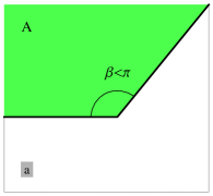
Figure 1: Dihedral confinement for the particles. In the region $\mathcal{A}$ in light-gray (green) particles are free to move while the region in white is forbidden. Note that no matter the value of the opening angle both light-gray (green) and white regions have dihedral shape. The dihedral shape of $\mathcal{A}$ determines that both Figs. a and b are straight-edge type confinements.

In next sections two different types of edge/wedge confinement will be analyzed. The dihedron $\mathcal{A}$, displayed in Fig. 1, corresponds to the region available for the center of each particle. This straight-edge confinement is defined by the Boltzmann factor $\exp\left[-\phi\left(\mathbf{r}\right)/kT\right]=\Theta\bigl{(}\left|\mathbf{r}-\mathcal{C}\right|\bigr{)}$, being $k$ the Boltzmann constant, $\Theta\bigl{(}x\bigr{)}$ the Heaviside function [$\Theta\bigl{(}x\bigr{)}=1$ if $x>0$ and zero otherwise], $\mathcal{C}=\mathcal{A}\setminus\mathbb{R}^{3}$ the complement dihedral region, and $\left|\mathbf{r}-\mathcal{C}\right|$ the shortest distance between $\mathbf{r}$ and $\mathcal{C}$.

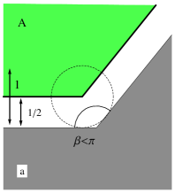
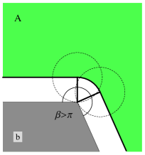
Figure 2: Dihedral and quasi-dihedral confinement induced on the fluid by a solid dihedron with solid-particle finite closest distance. Painted with darker gray is the solid dihedron, lighter gray (green) corresponds to the fluid and the empty region is in white. The draw in Fig. a is for the case $\beta<\pi$ while Fig. b corresponds to the case $\beta>\pi$. Dashed circles represent the hard repulsion wall-particle distance for particles lying near the edge. The arrows show characteristic lengths in $\sigma$ units. Note that $\mathcal{A}$ is a dihedron in Fig. a, i.e. it a a straight-edge confinement, even, $\mathcal{A}$ in Fig. b corresponds to a rounded-edge confinement.

A different type of confinement is defined by the Boltzmann factor $\exp\left[-\phi\left(\mathbf{r}\right)/kT\right]=\Theta\left(\left|\mathbf{r}-\mathcal{C}\right|-\frac{\sigma}{2}\right)$ with $\mathcal{C}$ the solid dihedral region and $\frac{\sigma}{2}$ the minimum solid-particle distance. This last case is drawn in Fig. 2 where $\mathcal{C}$ is dark and the forbidden region between $\mathcal{A}$ and $\mathcal{C}$ is shown in white. From a comparison between Fig. 1 and Fig. 2 one notes that region $\mathcal{A}$ is a dihedron not only in Figs. 1 a and b, but also in Fig. 2 a. Therefore, the case represented in Fig. 2a also corresponds to a straight-edge confinement. On the contrary, the region $\mathcal{A}$ shown in Fig. 2b is not a dihedron because $\mathcal{A}$ has a curved end-of-fluid surface. This situation corresponds to a rounded-edge confinement. Since Eq. (1) was originally derived for straight-edges, its extension to include the rounded-edge case is presented in Sec. IV.2. Note that the above discussion regarding different type of edge/wedge confinements essentially concerns to the confining potential but not with the inter-particles potential.

III Thermodynamics of a fluid in a edge/wedge confinement

To analyze the thermodynamic properties of the systems presented in Figs. 1 and 2 it is necessary to adopt a reference region (RR) $\mathcal{R}$. It should be underlined that for studying inhomogeneous fluids is crucial to clearly establish the adopted $\mathcal{R}$, which fixes the position and shape of the surface of tension, $\partial\mathcal{R}$. This issue is as fundamental as to clearly establish the system of reference in the study of a mechanical system. In this work it is adopted the density based RR (d-RR), i.e. the region where the one-body density distribution is non-null. This is in fact the region $\mathcal{A}$ shown in Figs. 1 and 2.

Let us consider a fluid confined by a hard wall edge at fixed $T$ and chemical potential $\mu$. Its grand potential taken with regard to the d-RR with measures $M=\left(V,A,L\right)$ is given by

$$\Omega=-PV+\gamma A+\mathcal{T}L\>.$$ (2)

Here, $P$ is the pressure, $\gamma$ is the wall-fluid surface tension (or excess surface free-energy), and $\mathcal{T}$ is the edge-fluid line-tension (or excess line free-energy). Naturally, the Mayer series of the grand potential of the system is given by

$$\frac{\Omega}{kT}=-\sum_{i\geq 1}\frac{\tau_{i}}{i!}z^{i}\,,$$ (3)

where $z=\Lambda^{-3}\exp\!\left(\mu/kT\right)$ is the activity of the fluid and $\Lambda$ the de Broglie´s length. It is generally accepted that Eq. (3) is rigorous as long as condensation is excluded (see p.131 of the book of HillHill (1956)). Here it is sufficient to assume that it converges for $0<z<R$ (for some $R>0$). Since both Eqs. (1) and (2) are linear in the measures $M$, therefore, Eq. (3) gives the power series in $z$ representation of the intensive thermodynamic properties $P$, $\gamma$ and $\mathcal{T}$. The mean number of particles in the system is $N=-\frac{z}{kT}\,\frac{\partial\Omega}{\partial z}$, and thus one obtain

$$N = \rho V+\Gamma_{A}A+\Gamma_{L}L\,,$$ (4)

$$= \sum_{i\geq 1}i\frac{\tau_{i}}{i!}z^{i}\,,$$ (5)

here, $\Gamma_{A}$ is the excess adsorption per unit area (of the boundary of $\mathcal{A}$) and $\Gamma_{L}$ is the excess adsorption per unit length. Again, linear relations (1, 4) and the power series in $z$ shown in (5) enable us to obtain the power series of the densities $\rho(z)$, $\Gamma_{A}(z)$, and $\Gamma_{L}(z)$. A linear decomposition, similar to that found for $\Omega$ and $N$, is also obtained for the fluctuation $\sigma_{{}_{N}}^{\,2}\equiv\left\langle N^{2}\right\rangle-N^{2}=z\frac{\partial N}{\partial z}$. This provides the power series in $z$ for each term in $\sigma_{{}_{N}}^{\,2}$ that scales with $V$, $A$ and $L$. Further, standard methods enable to transform the power series in $z$ to power series in $\rho$.Hill (1956) Notably, from the Eqs. (2) to (4) and the thermodynamic definition of $N$ [see expression above Eq. (4)] one can deduce the Gibbs adsorption equation for the surface adsorption $\Gamma_{A}=-\partial\gamma/\partial\mu$ and also its analogous, the Gibbs adsorption equation for the linear adsorption

$$\Gamma_{L}=-\partial\mathcal{T}/\partial\mu\,.$$ (6)

The confinement of the systems drawn in Fig. 1 is purely characterized by the region $\mathcal{A}$ where the density distribution could be non-null. For this type of confinement the unique simple choice for RR is $\mathcal{A}$ itself. On the other hand, even when the systems shown in Fig. 2 can also be analyzed under the same density-based $\mathcal{R}$ other RR could be adopted. The relation between the thermodynamic properties obtained under different choices of $\mathcal{R}$ will be studied in a forthcoming paper. It is worthwhile to note that by adopting the density-based $\mathcal{R}$, the systems depicted in Fig. 1a and Fig. 2a are identical, and thus, they have identical properties.

IV Second order cluster integral for HS confined by wedges

Here I focus on the second cluster integral for a straight-edge confinement. In this first step I consider a system more general than the HS, in which a pair of particles interact through the potential $\psi\left(r\right)$ with finite range $\xi$ [$\psi(r>\xi)=0$]. For this case, the Eq. (1) also holds.Urrutia (2013) The Mayer’s function of the fluid confined in a region $\mathcal{A}$ is $f\left(r\right)=\exp\left[-\psi\left(r\right)/kT\right]-1$ while its second cluster integral readsHill (1956)

$$\tau_{2}=\int_{\mathcal{A}}f\left(r_{12}\right)d\mathbf{r}_{1}d\mathbf{r}_{2}\>,$$ (7)

with $\mathbf{r}_{1}$, $\mathbf{r}_{2}$ the position of each particle of the pair and $r_{12}$ the distance between them. Given that $\mathcal{A}$ has one edge with inner-dihedral angle $\beta$ (see Figs. 1 and 2a), the coefficient $c_{2}\left(\beta\right)$ is given byUrrutia (2013)

$$2c_{2}\left(\beta\right)=-2\int_{\mathcal{D}_{1}}g_{1}\left(x\right)d\mathbf{r}^{(2)}+\int_{\mathcal{D}_{2}}g_{2}\left(\mathbf{r}^{(2)}\right)d\mathbf{r}^{(2)}\>,$$ (8)

where $\mathbf{r}^{(2)}$ is in the plane orthogonal to the edge direction while $g_{1}(x)$ and $g_{2}(x)$ are partial integrals of $f\left(r_{12}\right)$. For the case $0<\beta<\pi/2$, the integration domains are

$$D_{1} = I\cup II\cup III\>,$$ (9)

$$D_{2} = I\cup II\>.$$ (10)

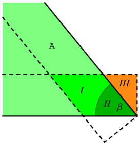
Figure 3: Detail of the straight-edge of $\mathcal{A}$ with $0<\beta<\pi/2$. In different gray-tones (green) are presented different regions near the edge. The integration domains $\mathcal{D}_{1}$ and $\mathcal{D}_{2}$ of Eq. (8) are dissected in the regions $I$, $II$ and $III$. Region $III$ (orange) is outside of $\mathcal{A}$.

Regions I, II and III are shown in Fig. 3. The continuous line shows the boundary of the region $\mathcal{A}$, $\partial\mathcal{A}$, which is defined by two planar faces. Parallel to each face, at a distance $\xi$, there is a plane plot with dashed line. A particle placed at $\mathbf{r}\in\mathcal{A}$ in the region between dashed and continuous parallel lines is surrounded by an sphere with radii $\xi$ that lies partially outside of $\mathcal{A}$. This sphere separates the interacting region from the non-interacting region.

From here on the analysis will only concern to the HS system and for simplicity I fixed the hard repulsion distance $\sigma=\xi=1$. For this system the volume and area coefficients of $\tau_{2}$ are: $b_{2}=-2\pi/3$ and $a_{2}=-\pi/8$. At present, the value of $c_{2}\left(\beta\right)$ is only known for two angles being $c_{2}(\pi/2)=-1/15$ and $c_{2}(3\pi/2)=-1/15$.Urrutia (2010) In addition, it is expected that $c_{2}\left(\beta\rightarrow\pi\right)=0$ due to the edge vanishes. Turning to Eq. (7), for HS $f\left(x\right)=-\Theta\left(1-x\right)$. By fixing $\mathbf{r}_{1}$, $f(\bigl{|}\mathbf{r}_{1}-\mathbf{r}_{2}\bigr{|})$ determines the so-called exclusion unit sphere (centered at $\mathbf{r}_{1}$) for which $f\left(r_{12}\right)$ is non-null. Concerning to the functions $g_{1}\left(\mathbf{r}\right)$ and $g_{2}\left(\mathbf{r}\right)$, they measure the volume of the portion of the exclusion unit sphere centered at $\mathbf{r}$ that lies outside of $\mathcal{A}$ when $\mathbf{r}$ is near to $\partial\mathcal{A}$.

$j$		$1$	$2$	$3$
f	$1$	$2$	$2$	$2$
e	$0$	$0$	$0$	$1$

Table 1: Pictures that represent the exclusion sphere, in dashed line, for different situations. The dark (blue) region is the overlap between the sphere and $\mathcal{A}$ while in lighter gray (lighter blue) is the region outside of $\mathcal{A}$.

Table 1 summarizes the different shapes that the outer portion of the exclusion sphere can take. There, f (e) is the number of faces (edges) intersected by the unit sphere, $j$ is an extra label for $\textrm{f}=2$, and for each $j$ corresponds a different $g_{\textrm{f},j}\left(\mathbf{r}\right)$ function. Given $\mathbf{r}$ and a face of $\mathcal{A}$, I define the $x$ as the normal coordinate of $\mathbf{r}$ relative to this face and positive in the inward direction. Thus, $g_{1}\left(x\right)$ is the volume of that part of the unit ball that lies in the semi-space with negative coordinate; i.e., if $x>1$ then $g_{1}\left(x\right)=0$, if $-1\leq x\leq 1$ then

$$g_{1}\left(x\right)=\frac{1}{3}\pi\left(2+x\right)\left(1-x\right)^{2}\>,$$ (11)

while for the case $x<-1$ $g_{1}\left(x\right)=4\pi/3$. On the other side, given a position $\mathbf{r}$ and a pair of intersecting faces that fix the coordinates $x$ and $x^{\prime}$, $g_{2}\left(\mathbf{r}^{(2)}\right)$ is the volume of the unit ball that lies in the region where at least one of these coordinates is negative. In the simple cases $g_{2}\left(\mathbf{r}^{(2)}\right)$ is equal to zero, $4\pi/3$, $g_{1}\left(x\right)$ or $g_{1}\left(x^{\prime}\right)$. For the less trivial cases and assuming that $x,x^{\prime}>0$ one has

$$g_{2}(\mathbf{r}^{(2)})=\begin{cases}g_{2,1}=g_{1}\left(x\right)+g_{1}\left(x^{\prime}\right)&\textrm{if }j=1\>,\\ g_{2,2}=g_{2,1}-4\pi/3&\textrm{if }j=2\>,\\ g_{2,3}=g_{2,1}-h\left(\mathbf{r}^{(2)}\right)&\textrm{if }j=3,\,\beta\leq\pi\,,\\ g_{2,3}=h\left(\mathbf{r}^{(2)}\right)&\textrm{if }j=3,\,\beta>\pi\,.\end{cases}\>$$ (12)

Here, $h(\mathbf{r}^{(2)})$ is the intersecting volume between the unit ball and the dihedron, that lies in the region where both coordinates are negatives. To make further progress I analyze the case $0<\beta<\frac{\pi}{2}$ for which $h\left(\mathbf{r}^{(2)}\right)=v\left(r,\theta\right)+v\left(r,\beta-\theta\right)$, with $r$ and $\theta$ the polar coordinates. An explicit expression for $v$ was obtained by Rowlinson.Rowlinson (1963) After taking into account trigonometric identities in Eq. (2.8) of Ref.Rowlinson (1963), the following expression for $v$ is obtained

$$v\left(r,\theta\right)=\text{ArcCot}\!\left[\frac{r\,\text{Cos}\left(\theta\right)}{\sqrt{1-r^{2}}}\right]\text{Sin}\left(\theta\right)\left(\frac{r^{3}}{3}\text{Sin}\left(\theta\right)^{2}-r\right)\!+$$

$$\>\>\frac{2}{3}\text{ArcTan}\!\left[\sqrt{1-r^{2}}\text{Tan}\left(\theta\right)\right]\!+\!\frac{r^{2}}{6}\sqrt{1-r^{2}}\text{Sin}\left(2\theta\right)\,.$$ (13)

Fig. 4 shows the exclusion sphere (dashed circle) near the edge for the case $\textrm{f}=2$ and $j=3$ ($0<\beta<\frac{\pi}{2}$) with $\mathbf{r}$ in the region $II$. There, the outer regions of the sphere with volumes $v\left(r,\theta\right)$ and $v\left(r,\beta-\theta\right)$ are also presented. If $\mathbf{r}$ is in the region $II$ then $g_{2}=g_{2,3}$ (as is the case of Fig. 4). On the other hand, if $\mathbf{r}$ is in the region $I$ then $g_{2}=g_{2,1}$.

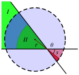
Figure 4: Exclusion sphere of radius $\sigma$ near the edge of $\mathcal{A}$ for $\mathbf{r}$ in region $II$. The outer region of the sphere with volume $v\left(r,\theta\right)$ is in lighter gray (pink) while that with volume $v\left(r,\beta-\theta\right)$ is dark (red).

Taking into account Eq. (10), the integral of $g_{2}\left(\mathbf{r}^{(2)}\right)$ over $D_{2}$ reduces to $2\int_{I\cup II}g_{1}\left(x\right)d\mathbf{r}^{(2)}-2\int_{II}v\left(r,\theta\right)d\mathbf{r}^{(2)}$. Using this expression and Eq. (9) to transform Eq. (8) one found

$$c_{2}\left(\beta\right)=-\int_{III}g_{1}\left(x\right)d\mathbf{r}^{(2)}-\int_{II}v\left(r,\theta\right)d\mathbf{r}^{(2)}\>.$$ (14)

The integral over region $III$ gives $\pi\cot\left(\beta\right)/15$. On the other hand, to solve the integral over region $II$ one introduces the change of integration variable $r\rightarrow\sqrt{1-s^{2}}$ to obtain $\left(1-\beta\cot\beta\right)/15$. Finally one found (for $0<\beta\leq\pi/2$)

$$c_{2}\left(\beta\right)=-\frac{1}{15}\left[1+\left(\pi-\beta\right)\cot\beta\right]\>.$$ (15)

In principle, the procedure can be reproduced for each of the ranges $\pi/2<\beta\leq\pi$, $\pi<\beta\leq 3\pi/2$, and $3\pi/2<\beta<2\pi$, but the expressions for $v$ become more complex, the domains of integration change, and the integral of $v$ becomes harder to solve. Thus, an alternative approach to analyze the range $\pi/2<\beta<2\pi$ is presented below (see Sec. IV.1). Here I advance the result: the Eq. (15) applies to the complete range $0<\beta<2\pi$.

IV.1 Other ranges of beta

With the aim of circumvent the integral on $v$, I will use a statistical-based analysis. Let us consider a region U of the space, composed by the disjoint union of regions A and B. If one drops a particle randomly in U the probability of finding it in A ($P_{\textrm{A}}$) or in B ($P_{\textrm{B}}$) relate by

$$1=P_{\textrm{A}}+P_{\textrm{B}}\>.$$ (16)

Let us consider a pair of (distinguishable) particles labeled as particle-$1$ and particle-$2$, randomly dropped in U. I will focus on the case where particles form a cluster (i.e., they lie at a distance $r<1$) and introduce $P_{\textrm{XY}}$ which is the probability that particle-$1$ lies in the region X while the particle-$2$ lies in the region Y. Thus, for the case of a pair of clustered particles one found the following relations

$$1 = P_{\textrm{AA}}+P_{\textrm{BB}}+2P_{\textrm{AB}}\>,$$ (17)

$$P_{\textrm{AA}} = P_{\textrm{AU}}-P_{\textrm{AB}}\>,$$ (18)

$$P_{\textrm{BB}} = P_{\textrm{BU}}-P_{\textrm{BA}}\>,$$ (19)

with $P_{\textrm{AB}}=P_{\textrm{BA}}$. Each of these probabilities is related to the volume of the coordinates phase space that corresponds to a cluster integral by the expression

$$P_{\textrm{XY}}=\tau_{\textrm{XY}}/\tau_{\textrm{UU}}\>.$$ (20)

Here $\tau_{\textrm{XY}}$ is the second cluster integral with the restriction that particle-$1$ is in X while particle-$2$ is in Y (with $\tau_{\textrm{XY}}=\tau_{\textrm{YX}}$). Thus, any of the Eqs. (17) to (19) can be translated to a relation between cluster integrals.

Let the region U be the semi-space S that is partitioned in two wedge-shaped regions labelled A and B with dihedral angles $\beta$ and $\beta^{\prime}=\pi-\beta$ (with $0<\beta<\frac{\pi}{2}$), respectively, as it is indicated in Fig. 5a.

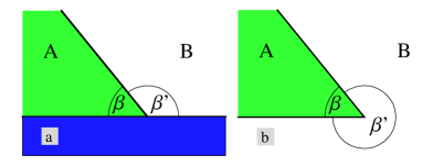
Figure 5: Picture showing the statistical-based approach to relate the edge term of $\tau_{2}\left(\mathcal{A}\right)$ with that of $\tau_{2}\left(\mathcal{B}\right)$. Dihedral region $\mathcal{B}$, with opening angle $\beta^{\prime}$, is in white. For the region $\mathcal{A}$ (green) with $\beta<\pi/2$, the term $c_{2}\left(\beta\right)$ is given in Eq. (15). Subfigure a is for the case of supplementary angles $\beta+\beta^{\prime}=\pi$ with $\frac{\pi}{2}<\beta^{\prime}<\pi$, while Subfigure b is for the case of add-full angles $\beta+\beta^{\prime}=2\pi$ with $\pi<\beta^{\prime}<2\pi$.

Based on Eqs. (17) and (20), the cluster integral $\tau_{2}$ for the system constrained to different regions are related one to each other. Thus, one finds

$$\tau_{\textrm{SS}}=\tau_{\textrm{AA}}+\tau_{\textrm{BB}}+2\tau_{\textrm{AB}}\>,$$ (21)

and from Eq. (1)

$$\tau_{\textrm{SS}} = 2b_{2}V_{\textrm{S}}-2a_{2}A\>,$$ (22)

$$\tau_{\textrm{AA}} = 2b_{2}V_{\textrm{S}}\frac{\beta}{\pi}-2a_{2}A+2c_{2}\left(\beta\right)L\>,$$ (23)

$$\tau_{\textrm{BB}} = 2b_{2}V_{\textrm{S}}\frac{\beta^{\prime}}{\pi}-2a_{2}A+2c_{2}\left(\beta^{\prime}\right)L\>,$$ (24)

where $V_{\textrm{S}}$ is the volume of the semi-space, $A$ is the area of the infinite plane, and $L$ is the length of the straight line. Eqs. (21, 22, 23) and (24) imply that $\tau_{\textrm{AB}}$ should be a linear function in $V_{\textrm{S}}$, $A$ and $L$. In fact, by equating term by term in Eq. (21) it is obtained

$$\tau_{\textrm{AB}}=-a_{2}A+2c_{mix}\left(\beta\right)L\>,$$ (25)

with $c_{mix}\left(\beta\right)=\frac{1}{2}\left[c_{2}\left(\beta\right)+c_{2}\left(\beta^{\prime}\right)\right]$ which is symmetric in the angles, i.e. $c_{2mix}\left(\beta\right)=c_{2mix}\left(\beta^{\prime}\right)$. On the same basis, Eqs. (18) and (19) are equivalent to

$$\tau_{\textrm{AA}} = \tau_{\textrm{AS}}-\tau_{\textrm{AB}}\>,$$ (26)

$$\tau_{\textrm{BB}} = \tau_{\textrm{BS}}-\tau_{\textrm{AB}}\>,$$ (27)

which shows that $\tau_{\textrm{AS}}$ and $\tau_{\textrm{BS}}$ are both linear in $V_{\textrm{S}}$, $A$ and $L$. Moreover, by combining the Eqs. (26, 27) and (21) one found

$$\tau_{\textrm{SS}}=\tau_{\textrm{AS}}+\tau_{\textrm{BS}}\>.$$ (28)

Finally, one introduces $2c_{aux}\left(\beta\right)$ and $2c_{aux}\left(\beta^{\prime}\right)$ as the $L$ coefficients in $\tau_{\textrm{AS}}$ and $\tau_{\textrm{BS}}$, respectively. Therefore, Eq. (28) shows that $c_{aux}$ is antisymmetric in the angles, i.e. $c_{aux}\left(\beta^{\prime}\right)=-c_{aux}\left(\beta\right)$. It is clear that if $c_{aux}\left(\beta\right)$ is known one can obtain $c_{aux}\left(\beta^{\prime}\right)$, $c_{mix}\left(\beta\right)$ and also $c_{2}\left(\beta^{\prime}\right)$. An interesting point is that $\tau_{\textrm{AS}}$ [related to $c_{aux}\left(\beta\right)$] is simpler to solve than any of the integrals $\tau_{\textrm{BB}}$, $\tau_{\textrm{AB}}$ or $\tau_{\textrm{BS}}$ [related to $c_{2}\left(\beta^{\prime}\right)$, $c_{mix}\left(\beta\right)$ and $c_{aux}\left(\beta^{\prime}\right)$, respectively] because in $\tau_{\textrm{AS}}$ the particle-2 is basically unconstrained while the particle-$1$ is constrained to A and thus the analysis done in the first part of Sec. II can be used. Utilizing an approach similar to that adopted in Ref. Urrutia (2013) to obtain Eq. (1), it is found $\tau_{\textrm{AS}}=2b_{2}V_{\textrm{S}}\frac{\beta}{\pi}-a_{2}A+2c_{aux}\left(\beta\right)L$ with $c_{aux}\left(\beta\right)=\frac{1}{2}\int_{III}g_{1}\left(z\right)d\mathbf{r}^{(2)}$ [see Eq. (14)]. Therefore, $c_{aux}\left(\beta\right)=\frac{\pi}{30}\cot\beta$ and $c_{mix}\left(\beta\right)=c_{2}\left(\beta\right)$ for all the range $0<\beta<\pi$. Even more, $c_{2}\left(\beta^{\prime}\right)=-\frac{1}{15}\left[1-\left(\pi-\beta^{\prime}\right)\cot\beta^{\prime}\right]$. This is exactly the same expression given in Eq. (15), i.e., we have shown that Eq. (15) applies in the extended domain $0<\beta<\pi$.

The same approach enable us to study the case $\pi<\beta<2\pi$. In Figure 5b it is shown the partition of the real space U in two dihedrons with inner angles $\beta$ and $\beta^{\prime}=2\pi-\beta$, respectively. The Eqs. (17) to (21), that relate probabilities and cluster integrals in different regions are still valid with the label S replaced by label U, and

$$\tau_{\textrm{UU}}=2b_{2}V\>,$$ (29)

where $V$ is the volume of the complete space. Thus, following the same procedure described above one notes that Eqs. (23) to (28) still apply, by changing $V_{\textrm{S}}$ by $V$ and $1/\pi$ by $1/2\pi$, while $A$ and $L$ remain unchanged. By combining Eqs. (26) and (27) one obtains

$$\tau_{\textrm{BB}}=\tau_{\textrm{BU}}+\tau_{\textrm{AA}}-\tau_{\textrm{AU}}\>.$$ (30)

In this case $\tau_{\textrm{AU}}=2b_{2}V\frac{\beta}{2\pi}$ and $\tau_{\textrm{BU}}=2b_{2}V\frac{\beta^{\prime}}{2\pi}$, which implies $c_{2}\left(\beta^{\prime}\right)=c_{2}\left(\beta\right)$. Therefore,

$$c_{2}\left(\beta\right)=-\frac{1}{15}\left[1+\left(\pi-\beta\right)\cot\beta\right]\>,$$ (31)

is finally valid for all the range $0<\beta<2\pi$.

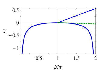
Figure 6: The edge/wedge coefficient of the second cluster integral, $c_{2}\left(\beta\right)$ for both straight- and rounded-edges. In continuous line (blue) is plot the straight-edge result given in Eq. (31). Other lines are for the rounded-edge case. In dashed line (blue) is plot $c_{2}\left(\beta\right)$ from Eq. (36) (curvature correction, d1-RR) while in dotted line (green) is plot $c_{2}\left(\beta\right)$ from Eq. (38) (curvature correction, d2-RR).

In Fig. 6, it is shown $c_{2}\left(\beta\right)$ for the straight- and rounded-edge, confinements. The expression for the straight-edge confinement, taken from Eq. (31), is plotted in continuous line. One observes that this $c_{2}\left(\beta\right)$ is non-positive, is symmetric around $\beta=\pi$, has smooth (analytic) behavior at $\beta\approx\pi$ where $c_{2}$ is zero, and diverges for both $\beta\rightarrow 0$ and $\beta\rightarrow 2\pi$. The results obtained in Sec. IV.2 for $c_{2}(\beta)$ of the rounded-edge confinement are also included in Fig. 6. There, two different flavors of the density based reference region are presented. In dashed line it is shown d1-RR while dotted line refers to d2-RR [Eqs. (36) and (38), respectively]. All the curves reach the zero value at vanishing edge/wedge with $\beta=\pi$.

IV.2 The rounded-edge

Here, I analyze the effect on the HS fluid produced by a solid dihedron that repel the core of each particle. Fig. 2 shows the edge of a solid dihedron with $\beta<\pi$ and with $\beta>\pi$ (Figs. 2a and 2b, respectively). There, the dark region constitutes the solid wall, in white is the excluded region induced on the HS fluid by the wall (forbidden for the particles center), and in lighter gray (green) is the available region for the center of particles, $\mathcal{A}$. In Fig. 2a one can observe that the dihedral walls induce near the edge a fluid-filled region $\mathcal{A}$ with dihedral shape, and therefore, the $c_{2}$ obtained above in Sec. IV.1 applies. On the contrary, in Fig. 2b the solid dihedron induces a curved end-of-fluid interface region with cylindrical shape and radius $1/2$. For this type of cylindrical-shape boundary of $\mathcal{A}$ it is necessary to analyze the decomposition of the cluster integrals. Following the procedure described in Ref.Urrutia (2013) and focusing on the HS fluid, in a first step one separates the integral domain $\mathcal{A}$ over bulk and skin regions (this last in the neighborhood of $\partial\mathcal{A}$). On a second step the planar faces domains are separated from that in the near-edge region of $\mathcal{A}$. Note that under this approach the surface area $A$ in Eqs. (1, 2) and (5) is the area of the planar region of $\partial\mathcal{A}$.

For the case of a rounded-edge confinement depicted in Fig. 2b the overall procedure leave us again with the expression given in Eq. (8), but now, $g_{2}$ is the volume of that part of the exclusion sphere outside of $\mathcal{A}$ when the intersection of the sphere with $\partial\mathcal{A}$ is non-planar. Moreover, the domains are given in terms of regions $II$, $II^{\prime}$ and $IV$ by

$$D_{1} = II\>,$$ (32)

$$D_{2} = II\cup II^{\prime}\cup IV\>.$$ (33)

These regions are shown in Fig. 7.

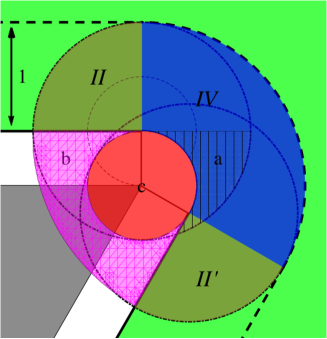
Figure 7: Details of the integration domains for a rounded-edge confinement, with $\beta>\pi$. Roman numbers ($II$, $II^{\prime}$ and $IV$) label the domain for $\mathbf{r}^{(2)}$ and $\mathbf{r}_{1}^{(2)}$ variables while small letters label the domain for $\mathbf{r}_{2}^{(3)}$.

Unfortunately, the involved integrals are not analytically solvable. I found convenient to write

$$2c_{2}\!\left(\beta\right)=-2\int_{II}\tilde{g}_{2}\left(x\right)d\mathbf{r}^{(2)}+\int_{IV}g_{2}\left(\mathbf{r}^{(2)}\right)d\mathbf{r}^{(2)}\>,$$

where $\tilde{g}_{2}\left(\mathbf{r}\right)$ is the volume of that part of the exclusion sphere (centered at $\mathbf{r}$) that lies in the region a (shaded zone in Fig. 7). These integrals may be expanded as double integrals to obtain

$$c_{2}\!\left(\beta\right)=G+Q\>,$$ (34)

with

$$G = \frac{1}{2}\int_{IV}\int_{\textrm{c}}H\,d\mathbf{r}_{2}^{(3)}d\mathbf{r}_{1}^{(2)}\>,$$

$$Q = \frac{1}{2}\int_{IV}\int_{\textrm{b}}H\,d\mathbf{r}_{2}^{(3)}d\mathbf{r}_{1}^{(2)}-\int_{II}\int_{\textrm{a}}H\,d\mathbf{r}_{2}^{(3)}d\mathbf{r}_{1}^{(2)}\>,$$ (35)

where $H=\Theta\bigl{(}1-\bigl{|}\mathbf{r}_{1}^{(2)}-\mathbf{r}_{2}^{(3)}\bigr{|}\bigr{)}$. The domains b and c are also drawn in Fig. 3. Finally, one solves $c_{2}$, $G$, and $Q$ for several values of $\beta$ by MonteCarlo numerical integration.Press (2007)

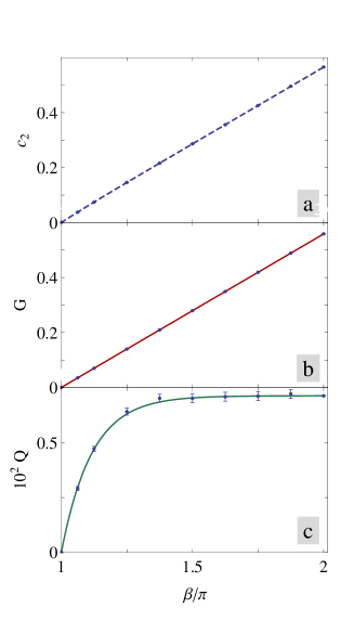
Figure 8: Obtained results for $c_{2}$, $G$ and $Q$. Error bars were drawn in each plot but in some cases are smaller than the point size. The meaning of each line is explained in the text.

In Fig. 8 (parts a, b and c) these results are shown. In Fig. 8a and b the nearly-linear behavior of the points of $c_{2}\!\left(\beta\right)$ and $G$, respectively, is apparent. To evaluate the slope of $G$ one takes circular coordinates $d\mathbf{r}_{1}^{(2)}=r_{1}dr_{1}d\theta$ and integrates numerically over $d\mathbf{r}_{2}^{(3)}r_{1}dr_{1}$ at arbitrary fixed angle $\theta$. The result is $G\simeq 0.17777(3)\left(\beta-\pi\right)$. This slope coincides with the exact result $\frac{\pi}{16}*{}_{2}F_{1}\!\left(-\frac{1}{2},\frac{1}{2};3;1\right)=\frac{8}{45}$ taken from the dependence of $\tau_{2}$ on the area of the lateral surface of a cylinder with radius $\frac{1}{2}$ [from Eq. (27) in Ref. Urrutia (2010)], where ${}_{2}F_{1}$ is the Hypergeometric function (sometimes denoted $F$). In Fig. 8b the exact dependence $G=\frac{8}{45}\left(\beta-\pi\right)$ is also plotted. A small deviation of $c_{2}\!\left(\beta\right)$ from the linear behavior is caused by $Q$, which is shown in Fig. 8c with the abscissa axes augmented in a factor $10^{2}$. I fit the points using an exponential form with two adjusting parameters and find $Q=0.007125\left\{1-\exp\left[-2.74\left(\beta-\pi\right)\right]\right\}$, which is included in Fig. 8c. Therefore, the result for $\beta>\pi$ is

$$c_{2}\!\left(\beta\right)=\frac{8}{45}\left(\beta-\pi\right)+Q\>,$$ (36)

which is shown in dashed-line in Fig. 8a. This expression describes with high precision the results of numerical integration. For comparison, Eq. (36) is also plotted in Fig. 6 using a dashed line. The two main differences with respect to Eq. (31) are: its positiveness and its finite value attained in the limit $\beta\rightarrow 2\pi$. This approach, that focus in the surface area of the planar part of $\partial\mathcal{A}$, is appointed as d1-RR.

To further analyze the obtained $c_{2}\left(\beta\right)$ in d1-RR one can write the edge term of $\tau_{2}/2$ emphasizing its dependence on the area of the cylindrical surface $A_{\textrm{cyl}}=\left(\beta-\pi\right)\frac{1}{2}L$. I found

$$c_{2}\!\left(\beta\right)\,L=-a_{2,\textrm{cyl}}A_{\textrm{cyl}}+Q\,L\>,$$ (37)

with the coefficient for the cylindrical surface area, $a_{2,\textrm{cyl}}=-\frac{16}{45}=-0.3555$. One observes that the behavior of $c_{2}\!\left(\beta\right)\times L$ is driven by its linearity with the surface area, which resembles the area dependence of $\tau_{2}$ and has the same sign. Alternatively, Eq. (37) suggest that one may adopt a slightly different RR by focusing on the total surface area of $\partial\mathcal{A}$. Once the contribution $-a_{2}A_{\textrm{cyl}}$ is added (and subtracted) to $\tau_{2}$ one obtains

$$c_{2}\!\left(\beta\right)=\left(\frac{8}{45}-\frac{\pi}{16}\right)\left(\beta-\pi\right)+Q\>,$$ (38)

that is designated by d2-RR. Note that under this approach the surface area $A$ in Eqs. (1, 2, 5) is the total area of $\partial\mathcal{A}$ that complains both, the planar and cylindrical surfaces. It is interesting to highlight that Eq. (36) and Eq. (38) describe the rounded-edge confinement shown in Fig. 2b. The difference lies in the adopted dissection of $\partial\mathcal{A}$.

V Results

Turning to the thermodynamic properties of the HS system confined by a single edge/wedge, they can be expanded as power series in $z$ and then as power series in $\rho$. From here on, I truncate all the series to second order and thus terms of order $O(z^{3})$ and $O(\rho^{3})$ are depreciated. Taking into account the known values of $b_{2}$ and $a_{2}$, one finds for the low density regime:

$$P/kT=\rho+\rho^{2}2\pi/3\>,$$

$$\gamma/kT=-\rho^{2}\pi/8 \Gamma_{A}=\rho^{2}\pi/4\>.$$ and (39)

These expressions correspond to the known expansions, of the pressure of a bulk HS fluid, of the fluid-wall surface tension, and of the fluid-wall surface adsorption (when a HS fluid is confined by a planar hard-wall), respectively. Furthermore, the correspondence between the obtained series for $P$, $\gamma$ and $\Gamma_{A}$, and the known series expansions also apply when higher order terms in $z$ and $\rho$ are considered. Therefore, Eq. (39) helps to define accurately the meaning of the intensive magnitudes introduced in Eqs. (2) and (4). The line-thermodynamic properties of the HS fluid confined by an edge/wedge are

$$\mathcal{T}/kT=-c_{2}\rho^{2} \Gamma_{L}=2c_{2}\rho^{2}\>.$$ and (40)

From simple inspection of Eqs. (39) and Eq. (40), one notes that $\gamma/kT$ ($\mathcal{T}/kT$) is minus one half of $\Gamma_{A}$ ($\Gamma_{L}$). It is interesting to note that using the Gibbs adsorption equations [see Eq. (6)] up to terms of order $z^{2}$ one finds

$$\gamma/kT=-\Gamma_{A}/2 \mathcal{T}/kT=-\Gamma_{L}/2\>.$$ and (41)

Therefore, these remarkable relations (that holds up to terms of order $\rho^{2}$) does not only apply to the HS fluid, but also, to any fluid confined by hard-wall edges and wedges. In fact, as long as $\tau_{i}$ were given by Eq. (1), the relations in Eq. (41) should be also valid for planar walls and wedges that interact with the particles trow a less trivial external potential $\phi\left(\mathbf{r}\right)$ than the infinite repulsion. The adsorption equations given in Eq. (41) are very similar to the ideal gas equation of state $P/kT=\rho$ in several aspects. In particular, they are simple relations between free-energy densities, number densities and temperature, i.e. they are simple equations of state of the adsorbed gas. These ideal-adsorption equations include terms up to order $\rho^{2}$, terms of the same order are not included in the pressure of the ideal gas.

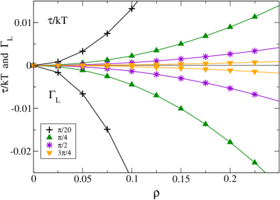
Figure 9: Line adsorption and line tension (scaled with temperature) for the straight-edge confinement at four angles in the range $0<\beta<\pi$. Line adsorption curves lie in the negative abscissa region, while line tension curves lie in the positive ones.

In Fig. 9 the density dependence of line tension (scaled with temperature) and line-adsorption for several edges/wedges with $\beta<\pi$, are shown (see Figs. 1a and 2a). Different curves correspond to four different angles. There, the line tension curves are positive but line adsorption ones are negatives. The curves for larger values of $\beta$ are near to the zero ordinate axis, which corresponds to the limiting case $\beta=\pi$ of an edge that vanishes in an infinite planar wall. On the contrary, in the limit $\beta\rightarrow 0$ both $\mathcal{T}/kT$ and $\Gamma_{L}$ diverge (not shown in the Figure) because $c_{2}(\beta)$ diverges. This can be rationalized as the impossibility of attaining the dimensional crossover to the hard disc system with Eq. (36) because an extra non-analytic term should appears in the case of $\beta\rightarrow 0$. This was previously verified for the HS system under confinement in box-shaped cavities.Urrutia (2010) Note that, no matter the value of $\beta$ (in the range $0<\beta<\pi$) the HS system apparently desorbs from the edge/wedge region (it has a negative adsorption). This unexpected behavior comes from the direct analysis of the pure line-adsorption term $\Gamma_{L}$ given in Eq. (4). I will return to this point at the end of this section.

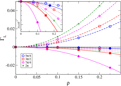
Figure 10: Line adsorption for both, the straight- and rounded-edges confinement, at angles in the range $\pi<\beta\leq 2\pi$. Continuous lines (with filled symbols) show results for the straight-edge confinement while dashed and dotted lines correspond to rounded-edge (d1-RR and d2-RR, respectively).

Fig. 10 presents the behavior of line-adsorption with density for different edges/wedges that correspond to $\beta>\pi$. In the inset, the details of a region near the horizontal axis is shown. Straight lines correspond to the straight-edge confinement (see Fig. 1b) while discontinuous lines correspond to the rounded-edge case (see Fig. 2b). The dashed and dotted lines correspond to the different criteria adopted for the dissection of $\partial\mathcal{A}$, d1-RR and d2-RR, respectively. I wish to note some interesting features of Fig. 10 that follows from the obtained $c_{2}\left(\beta\right)$ results (see Fig. 6). First, one observes that for a fixed $\beta$ (and considering d1-RR), the pure line-adsorption on straight- and rounded-edges are very different (they have opposite sign). Second, for the rounded-edge the line-adsorption obtained using d1-RR differs strongly from that obtained by using d2-RR. Thus, based on these issues one concludes that straight-edges behaves very different to rounded-edges, and also, that given a fixed physical constraint the adoption of different RRs may produce strongly different results. A third noticeable characteristic is that straight-edges show apparent desorption for any (nontrivial) dihedral angle. A comparison between Fig. 9 and Fig. 10 shows that this apparent desorption is symmetric around $\beta=\pi$, i.e. $\Gamma_{L}(\pi-\Delta\beta)=\Gamma_{L}(\pi+\Delta\beta)$.

Turning to Fig. 10, one notes that in all cases the curves for smaller values of $\beta$ are nearer to the zero ordinate axis (which gives the limiting planar-wall case $\beta=\pi$ of a vanishing edge). The other interesting limit for $\Gamma_{L}$ is $\beta\rightarrow 2\pi$. There, the curve for the rounded-edge does not diverge, but $\Gamma_{L}$ for the straight-edge diverges (not shown in the figure) because $c_{2}(\beta)$ [see Eq. (8)] diverges too. This can be rationalized again by recognizing that Eq. (36) is unsuitable to analyze the confinement produced by a vanishing straight-wedge, because an extra non-analytic term should appear in the case of $\beta\rightarrow 2\pi$. In this limit of the straight-edge case, the available region for the fluid $\mathcal{A}$ becomes the complete space with volume $V$ (in fact one should subtract half plane, that has zero volume measure), and thus, the homogeneous system result $\tau_{2}=2b_{2}V$ should be recovered.

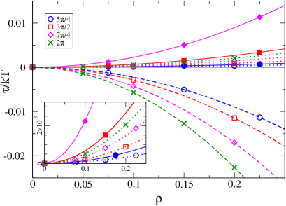
Figure 11: Line tension (scaled with temperature) for both, the straight- and rounded-edges confinement for four angles in the range $\pi<\beta\leq 2\pi$. See details in Fig. 10.

In Fig. 11 the dependence of line-tension with density for different edges/wedges with $\pi<\beta\leq 2\pi$, is shown. The inset shows a detail of a region near the axis. One notes that for the straight-edge confinement the line tension (i.e. the line component of the Grand free-energy) monotonically increases with increasing $\beta$ (from $\beta=\pi$) and diverges for all densities at $\beta\rightarrow 2\pi$ because this limit can not be described by Eq. (8). The reasons of this behavior are the same discussed in the case of Fig. 10. Other features observed in Fig. 11 follow the characteristics noted for the curves in Fig. 10. Perhaps, the most interesting result about $\mathcal{T}$ is not in the plotted curves in Fig. 11 but on the existence of the analytic expression for $\mathcal{T}$, in fact, it enable us to give the analytic expression of the grand free energy $\Omega\left(\beta,\rho\right)$ up to order $\rho^{2}$.

The unexpected apparent desorption and symmetry of $\Gamma_{L}$ for system confined by a straight-edge, and the strong dependence of $\Gamma_{L}$ on the adopted RR for system confined by a rounded-edge, both suggest an alternative approach to analyze the adsorption produced by edges and wedges. I realize that a more meaningful definition of edge/wedge adsorption that considers finite volumes and sets as reference the planar wall is possible. Thus, I introduce the mean excess of adsorbed density

$$\Delta\rho = N(r)/V(r)-\rho\>.$$ (42)

where $N(r)$ is the mean number of particles in a suitably selected region with volume $V(r)$ and thickness $r$. A similar approach enable us to introduce the mean excess of free-energy density

$$\Delta\omega = \Omega(r)/V(r)+P\>,$$ (43)

here $\Omega(r)$ is the free-energy of the $N\left(r\right)$ particles in $V\left(r\right)$. Both $\Delta\rho$ and $\Delta\omega$ quantify the local behavior of the HS system in the neighborhood of the apex. The analytic expressions of the mean excess densities $\Delta\rho$ and $\Delta\omega$ for the straight-edge and for the rounded-edge are deduced in the Appendix A.

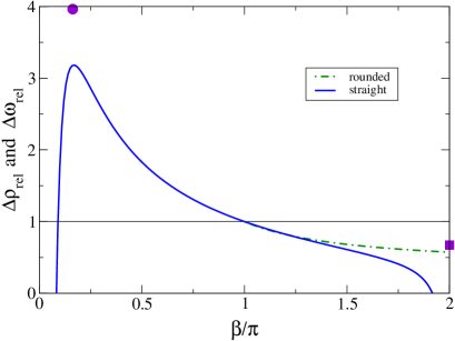
Figure 12: Relative mean excess adsorbed density and free-energy density in the neighborhood of the edge/wedge divided by its planar wall value. $\Delta\rho_{rel}=\Delta\omega_{rel}$ and they are independent of the density up to the considered order.

Both, $\Delta\rho$ and $\Delta\omega$ are proportional to $\rho^{2}$ (terms of higher order are not considered in current work). Under the adopted truncation of terms $O(\rho^{3})$ the distance between $\partial\mathcal{A}$ and the zone of the spatial density distribution where it attains its bulk value $\rho$ is $1$, thus, I fixed $r=1$. It is convenient to introduce the relative mean excess values of the adsorbed density and free-energy density,

$$\Delta\rho_{rel}=\frac{\Delta\rho}{\Delta\rho_{wall}}\>\textrm{and}\>\Delta\omega_{rel}=\frac{\Delta\omega}{\Delta\omega_{wall}}\>,$$ (44)

respectively. One can note some properties of $\Delta\rho_{rel}$ and $\Delta\omega_{rel}$: they are independent of the number density $\rho$ and only depend on $\beta$, their analytic expressions are the same i.e. $\Delta\rho_{rel}=\Delta\omega_{rel}$, and if the d2-RR is adopted (in place of d1-RR) the expressions for $\Delta\rho_{rel}$ and $\Delta\omega_{rel}$ remain unmodified. An important difference between $\Delta\rho_{rel}$ and $\Delta\omega_{rel}$ is the sign of the denominator in Eq. (44). Given that $\Delta\rho_{wall}>0$ it follows that $\Delta\rho_{rel}>0\Leftrightarrow\Delta\rho>0$. On the contrary, $\Delta\omega_{wall}<0$ and thus it follows that $\Delta\omega_{rel}>0\Leftrightarrow\Delta\omega<0$. This implies that a maximum in $\Delta\omega_{rel}$ indicates a minimum in $\Delta\omega$. In Fig. 12 the relative magnitudes $\Delta\rho_{rel}$ and $\Delta\omega_{rel}$ are plotted. Continuous line shows the result for the straight-edge confinement [see Eq. (50)] while the dot-dashed line corresponds to the rounded-edge. Note that, the symmetry found in $c_{2}(\beta)$, $\Gamma_{L}$ and $\mathcal{T}/kT$ for the straight-edge [$c_{2}(\beta)=c_{2}(2\pi-\beta)$ for $0<\beta<\pi$] disappears in $\Delta\rho_{rel}$ and $\Delta\omega_{rel}$. The curves show that in the neighborhood of a very acute edge ($0<\beta\lesssim 0.091\pi$) the HS gas desorbs, as it also happens for the gas near a solid wedge ($\beta>\pi$). In the intermediate range $0.091\pi\lesssim\beta<\pi$ that includes acute and obtuse edges the HS gas adsorbs, with a peak of maximum adsorption at $\beta\approx 0.17\pi$ with $\Delta\rho_{rel}\approx 3.2$. All these trends agree with that found in Ref. Schoen and Dietrich (1997), where the single bulk density $\rho=0.7016$ (which is not a small density because fluid-solid transition is at $\rho\approx 1$) was studied using free-energy density functional theory (DFT). Besides, the local mean density of free-energy relative to the planar-wall condition follows exactly the same behavior that shows $\Delta\rho_{rel}$, which implies a minimum of mean excess of free-energy density $\Delta\omega$ at $\beta\approx 0.17\pi$. The results presented in Fig. 12 slightly depend on the details of the adopted region $V(r)$ and on the adopted value of $r$. Although, the discussed general trends remain unmodified. As an indication of this feature, the values obtained using a different definition of $V\left(r\right)$ are shown with a small circle (the maximum) and a small square (the rounded-edge value for $\beta=2\pi$). More details are given in Appendix A.

V.1 Adsorbed HS gas on a Corrugated wall

The results shown in Fig. 12 motivated the study of a more complex geometrical confinement than edges and wedges. Here, I analyze the properties of the HS gas on contact with a corrugated wall in the low density regime, by focusing in the total adsorption and surface free-energy of the system. Adsorption is an easy measurable magnitude accessible through experiments, through a variety of simulations techniques (molecular dynamics and MonteCarlo) and also using DFT. On the other hand, the surface free-energy density is not simple to measure in experiments but it can be approximately evaluated by DFT. Together, they provide a variety of quantitative and high-precision tests between different approaches.

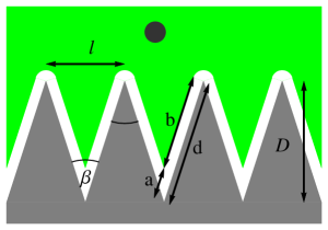
Figure 13: Scheme of the corrugated wall built by acute straight-edges (grooves) and rounded-edges (ridges).

In Fig. 13 a draw of the system with its principal lengths is shown and a single HS particle is included. There, $l$ is the distance between cups and $D$ is the depth. Lengths $a$, $b$, and $d$ are used to calculate the relevant areas in Appendix B. This complex-shape confinement includes rounded-edges as that shown in Fig. 2b. In the analysis it is adopted the d1-RR point of view. Given a planar wall of area $A_{0}$, the number of adsorbed particles per unit area is simply $N_{A}/A_{0}=\Gamma_{A}$. For a corrugated wall scratched on the planar wall one defines the effective adsorption

$$\Gamma_{eff}=\frac{N_{A}}{A_{0}}=\Gamma_{A}\frac{A}{A_{0}}+\left(\Gamma_{L}+\Gamma_{L}^{{}^{\prime}}\right)\frac{L_{tot}}{A_{0}}\>,$$ (45)

with $\Gamma_{L}$ the line adsorption of the groove edge ($\beta<\pi$), $\Gamma_{L}^{{}^{\prime}}=\Gamma_{L}(2\pi-\beta)$ the line adsorption of the ridge edge, and $L_{tot}$ the total length of the edges with dihedral angle $\beta$. For the analyzed HS system the magnitudes $\Gamma_{A}$ and $\Gamma_{L}$ were given in Eqs. (39, 40), while the analytic expressions of $A$ and $A_{0}$ as functions of $\beta$ and $D$ are evaluated in the Appendix B. Following the same approach one defines the effective surface density of free-energy

$$\gamma_{eff}=\frac{\Omega_{A}}{A_{0}}=\gamma\frac{A}{A_{0}}+\left(\mathcal{T}+\mathcal{T}^{{}^{\prime}}\right)\frac{L}{A_{0}}\>,$$ (46)

with $\Omega_{A}=\Omega+PV$ and $\mathcal{T}^{{}^{\prime}}=\mathcal{T}\left(2\pi-\beta\right)$. Both $\Gamma_{eff}$ and $\gamma_{eff}$ are proportional to $\rho^{2}$ and depend on a non-trivial way on $\beta$ and $D$. On the other hand, the relative adsorption and the relative surface density of free-energy

$$\Gamma_{rel}=\frac{\Gamma_{eff}}{\Gamma_{A}}\>\textrm{and}\>\gamma_{rel}=\frac{\gamma_{eff}}{\gamma}\>,$$ (47)

respectively, are both independent of $\rho$. Also, they are identical i.e. $\Gamma_{rel}=\gamma_{rel}$.

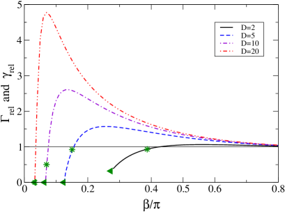
Figure 14: Relative adsorption and relative free-energy per surface area for the corrugated wall as a function of dihedral angle of the groove edge. $\Gamma_{rel}=\gamma_{rel}$ and they are independent of the density up to the considered order. Curves for several values of the depth $D$ are shown.

In Fig. 14 $\Gamma_{rel}$ and $\gamma_{rel}$ are presented as functions of $\beta$ and $D$. In the limit of vanishing edge ($\beta\rightarrow\pi$) they go, naturally, to one. On the contrary, for very small dihedral angles curves show that the system desorbs from the corrugated wall ($\Gamma_{rel}<1$) and consistently the relative surface density of free energy also becomes smaller than one. In the intermediate angular range the relative adsorption (and the relative free energy) has a peak which becomes more and more pronounced and goes to smaller values of $\beta$ as $D$ increase. A cutoff on the confidence of the plotted curves is introduced through the use of stars and triangles. Stars show the smaller value of $\beta$ (for each $D$) beyond that the ridge and the groove become so nearer that their interference could be noted (it was estimated using the condition $b>1$). This interference becomes relevant for corrugated walls with short spatial periodicity length $l$. In such case an extra interference term $\Delta c_{2}$ that couples ridge and groove contributions should be considered. This term should compensate the divergence of $c_{2}\left(\beta\right)$ for very small angles ($\beta\rightarrow 0$). Plotted triangles mark the smaller value of $\beta$ (for each $D$) beyond that one expects that $\Delta c_{2}$ becomes the relevant term (it was estimated using the condition $b>0$). The evaluation of $\Delta c_{2}$ is beyond the scope of present work.

VI Final Remarks

In this work the thermodynamic properties of the confined HS fluid, which is a relevant reference system for both simple and colloidal fluids, was studied. The HS fluid was confined in wedges and by edges, and analyzed in the framework of the activity series expansion for the grand free energy. The coefficients of these series are the inhomogeneous version of the Mayer’s cluster integrals, which decompose linearly in terms of its volume, surface area, and edges length components. Two different type of edge/wedge confinement were analyzed: the straight-edge and the rounded-edge.

On the basis of this non-standard approach and using analytic grounds it was studied in the low density regime the dependence of the linear-thermodynamic properties on the dihedral angle. This analysis was done after obtaining the functional dependence of the second cluster integral, $\tau_{2}$, with the dihedral angle for the complete range $0<\beta<2\pi$ and for both types of edges. In particular, the second cluster edge component $c_{2}(\beta)$ was obtained by applying analytic and numerical integration schemes, and a statistical-based analysis.

The exact expression for $c_{2}(\beta)$ was derived in the case where the center of each particle lies in a straight-edge region. In addition, accurate analytic expressions for $c_{2}(\beta)$ were found in the case of a hard-wall wedge that induce a rounded-edge confinement ($\pi<\beta<2\pi$). The up to present unknown $c_{2}(\beta)$ allows to obtain the pure line-tension and line-adsorption of a single edge/wedge in terms of density power series up to order two. The analytic approach to the edge/wedge confined HS system was extended to evaluate the mean excess of, adsorbed density and free-energy density in the neighborhood of the edge, relative to the planar wall. Both properties exhibit an interesting peak at $\beta\approx\pi/6$ that corresponds to a maximum of adsorption and minimum of free-energy. Furthermore, formulas were also extended to analyze the HS system confined by a corrugated wall. In this case, it was observed an interesting non-trivial behavior of the effective adsorption and effective surface free-energy that develop an extremum as function of the dihedral angle and the depth of the corrugation.

Notably, the obtained results for HS are absolute in the sense that they do not involve any assumption about approximate equations of state for the bulk system, and thus, they constitute reference values for the validation and development of more accurate approximate theories for inhomogeneous fluid. Further, the expressions found for $c_{2}$ of HS suggest that the system of square well particles may be also studied by a direct extension of the developed scheme. Finally, concerning the HS system, both the statistical-based and the MonteCarlo approaches that were implemented to evaluate $c_{2}$ are promising to extend the studies to $c_{3}$ and $c_{4}$ (third and fourth cluster integrals).

Appendix A Mean excess densities $\Delta\rho$ and $\Delta\omega$ for a single edge/wedge

To obtain the analytic expressions of $\Delta\rho$ and $\Delta\omega$ one should choose a small and simple region around the apex. For this region with thickness $r$ one assumes that $\varOmega\left(r\right)$ and $N\left(r\right)$ have a linear form like those given in Eqs. (2, 4), in terms of measures $V\left(r\right)$, $A\left(r\right)$ and $L$. Therefore one finds

$$\Delta\rho=\frac{A\left(r\right)}{V\left(r\right)}\Gamma_{A}+\frac{L}{V\left(r\right)}\Gamma_{L}\>,$$ (48)

$$\Delta\omega=\frac{A\left(r\right)}{V\left(r\right)}\gamma+\frac{L}{V\left(r\right)}\mathcal{T}\>.$$ (49)

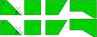
Figure 15: Regions used to evaluate the mean values over finite volumes, $\Delta\rho$ and $\Delta\omega$, for different values of the dihedral angle $\beta$.

For the straight-edge the adopted region is that part of a cylinder with radius $r$ and axis on the edge that intersects $\mathcal{A}$, as can be observed in Fig. 15 first row. Thus, $A(r)/V(r)=\frac{4}{\beta r}$ and $L/V(r)=\frac{2}{\beta r^{2}}$. For the rounded-edge I adopt d1-RR and take the region with volume $V(r)$ described in Fig. 7 as region $II+II^{\prime}+IV$ (with depth $r$ in place of $\sigma$). Therefore, $V\left(r\right)=L\left[\frac{\beta-\pi}{2}\left((r+\frac{1}{2})^{2}-\frac{1}{4}\right)+\frac{\pi}{2}r^{2}\right]$ and $A\left(r\right)=L2r$. Note that the truncated low order density expansion was not yet introduced in Eqs. (48, 49). Now, one replaces in Eq. (48) [Eq. (49)] $\Gamma_{A}$ and $\Gamma_{L}$ ($\gamma$ and $\mathcal{T}$) with the exact expressions up to order $\rho^{2}$ taken from Eqs. (39, 40). To fix the value of $r$ one relates it with the range of the inhomogeneous density profile consistent with the order $\rho^{2}$ truncation, i.e. $\sigma$. In principle it would be $r\gtrsim\sigma$ but for simplicity It is adopted $r=\sigma$. For the straight-edge one obtains the simple analytic expression

$$\Delta\rho_{rel}=\Delta\omega_{rel}=\frac{\pi}{\beta}+\frac{4}{\beta}c_{2}\>,$$ (50)

[$c_{2}$ is given in Eq. (15)] which is plotted in Fig. 14.

The above adopted region around the apex of the edge or wedge, is not the unique possible choice. A more subtle analysis shows that the following more complex alternative, which modifies $V\left(r\right)$ (but not the area $A\left(r\right)=L2r$), may be better. For the case of a straight-edge the regions are shown in Fig. 15 second row. One finds the volume definition: If $0<\beta<\pi/2$ then $V(r)=Lr^{2}\tan\left(\beta/2\right)$, if $\pi/2<\beta<\pi$ then $V(r)=Lr^{2}\left[2-\cot\left(\beta/2\right)\right]$, while if $\pi<\beta<2\pi$ then $V(r)=Lr^{2}\left[2+\beta/2\right]$. On the rounded-edge case, one adopts a region akin that depicted in Fig. 7 as region $II+II^{\prime}+IV$ but with $II$ and $II^{\prime}$ replaced by squares with sides of length $r$. It gives $V(r)=L\left[\frac{\beta-\pi}{2}\left((r+\frac{1}{2})^{2}-\frac{1}{4}\right)+2r^{2}\right]$. Finally one fixes $r=\sigma$.

Appendix B Relative adsorption and surface free-energy on a corrugated wall

The characteristic lengths used to develop explicit formulas for the areas $A_{0}$ and $A$ are presented in Fig. 13. The area of the planar wall surface of reference is $A_{0}=l*Ln$ where $n$ is the number of grooves separated by a distance $l$ that will be considered and $L_{tot}=Ln$. This planar wall is transformed to a corrugated wall by scratching. For the corrugated wall I adopt the d1-RR [see Eq. (36)] and thus the relevant area $A$ is the area of the planar part of the gas-wall interface. In terms of the lengths shown in Fig. 13 it is obtained: $A=2b*Ln$ with $b=d-a$, $a=\sigma\cot\left(\beta/2\right)$, $d=D\sec\left(\beta/2\right)$ and $l=2D\tan\left(\beta/2\right)$. Rearranging these identities one finds

$$A/Ln = 2\left[D\sec\left(\beta/2\right)-\sigma\cot\left(\beta/2\right)\right]\>,$$

$$A_{0}/Ln = 2D\tan\left(\beta/2\right)\>.$$ (51)

Once Eq. (51) is replaced in Eqs. (45, 46) one obtains

$$X_{rel}=\csc\left(\beta/2\right)-\frac{\sigma}{D}\cot\left(\beta/2\right)^{2}+y_{rel}\frac{1}{D}\cot\left(\beta/2\right)\>,$$ (52)

where the relative magnitude $X_{rel}$ is any of $\Gamma_{rel}$ and $\gamma_{rel}$, and $y_{rel}$ is $\left(\Gamma_{L}+\Gamma_{L}^{{}^{\prime}}\right)/\Gamma_{A}$ or $\left(\mathcal{T}_{L}+\mathcal{T}_{L}^{{}^{\prime}}\right)/\gamma_{A}$, in each case. Note that $\sigma$ is here related to the external confining potential, it is the minimum enabled distance between the center of the particle and the substrate. Naturally, for the HS fluid $\sigma$ is also the pair collision distance. The two points of view unify when one calls $\sigma$ as the particle diameter. Finally, for the HS up to order $\rho^{2}$ it is $y_{rel}=8\left[c_{2}\left(\beta\right)+c_{2}\left(2\pi-\beta\right)\right]/\pi$ with $c_{2}\left(\beta\right)$ and $c_{2}\left(2\pi-\beta\right)$ taken from Eqs. (15, 36). This implies that $X_{rel}$ becomes independent of $\rho$.

If the d2-RR is adopted in place of d1-RR, the relevant area for the corrugated wall turns to be $A/Ln=2b+\sigma\left(\pi-\beta\right)/2$ [see Eq. (38)]. Furthermore, $y_{rel}$ changes because $c_{2}\left(2\pi-\beta\right)$ is that of Eq. (38). These changes do not modify $X_{rel}$ and thus Fig. 14 also shows those results found under the adoption of d2-RR.

References

- Henderson (2002) J. R. Henderson, Physica A: Statistical Mechanics and its Applications 305, 381 (2002).
- Henderson (2004a) J. R. Henderson, The Journal of Chemical Physics 120, 1535 (2004a).
- Henderson (2004b) J. R. Henderson, Phys. Rev. E 69, 061613 (2004b).
- Boţan et al. (2009) V. Boţan, F. Pesth, T. Schilling, and M. Oettel, Phys. Rev. E 79, 061402 (2009).
- Schneemilch, Quirke, and Henderson (2003) M. Schneemilch, N. Quirke, and J. R. Henderson, The Journal of Chemical Physics 118, 816 (2003).
- Bryk et al. (2003) P. Bryk, R. Roth, M. Schoen, and S. Dietrich, EPL (Europhysics Letters) 63, 233 (2003).
- Schoen (2002) M. Schoen, Colloids and Surfaces A: Physicochemical and Engineering Aspects 206, 253 (2002).
- Henderson (2006) J. R. Henderson, Physical Review E 73, 010402 (2006).
- Almenar and Rauscher (2011) L. Almenar and M. Rauscher, Journal of Physics: Condensed Matter 23, 184115 (2011).
- Freed and Wu (2011) K. F. Freed and C. Wu, Journal of Chemical Physics 135, 144902 (2011).
- Lutsko (2012) J. F. Lutsko, The Journal of Chemical Physics 137, 154903 (2012).
- Statt et al. (2012) A. Statt, A. Winkler, P. Virnau, and K. Binder, Journal of Physics: Condensed Matter 24, 464122 (2012).
- Pusey and Megen (1986) P. N. Pusey and W. v. Megen, Nature 320, 340 (1986).
- Royall, Poon, and Weeks (2013) C. P. Royall, W. C. K. Poon, and E. R. Weeks, Soft Matter 9, 17 (2013).
- Mandal et al. (2014) S. Mandal, S. Lang, M. Gross, M. Oettel, D. Raabe, T. Franosch, and F. Varnik, Nat. Commun. 5, 4435 (2014).
- Kedzierski and Wajnryb (2011) M. Kedzierski and E. Wajnryb, The Journal of Chemical Physics 135, 164104 (2011).
- Hansen and McDonald (2006) J.-P. Hansen and I. R. McDonald, Theory of simple liquids, 3rd Edition (Academic Press, Amsterdam, 2006).
- Wang and Liu (2012) Z. Wang and L. Liu, Phys. Rev. E 86, 031115 (2012).
- Urrutia (2014) I. Urrutia, Phys. Rev. E 89, 032122 (2014).
- Urrutia and Castelletti (2012) I. Urrutia and G. Castelletti, The Journal of Chemical Physics 136, 224509 (2012).
- Urrutia and Pastorino (2014) I. Urrutia and C. Pastorino, The Journal of Chemical Physics 141, 124905 (2014).
- Urrutia (2010) I. Urrutia, The Journal of Chemical Physics 133, 104503 (2010).
- Hill (1956) T. L. Hill, Statistical Mechanics (Dover, New York, 1956).
- Bellemans (1962a) A. Bellemans, Physica 28, 493 (1962a).
- Bellemans (1962b) A. Bellemans, Physica 28, 617 (1962b).
- Urrutia (2013) I. Urrutia, ArXiv e-prints (2013), arXiv:1303.3468 [cond-mat.stat-mech] .
- Rowlinson (1963) J. S. Rowlinson, Molecular Physics 6, 517 (1963).
- Press (2007) W. Press, Numerical recipes: the art of scientific computing (Cambridge University Press, Cambridge, UK New York, 2007).
- Note (1) I have detected a misprint in Eq. (27) of Ref. Urrutia (2010). There, where it reads it should be .
- Schoen and Dietrich (1997) M. Schoen and S. Dietrich, Phys. Rev. E 56, 499 (1997).