An Effective Selection Method for Low-Mass Active Black Holes and First Spectroscopic Identification

Abstract

We present a new method to effectively select objects which may be low-mass active black holes (BHs) at galaxy centers using high-cadence optical imaging data, and our first spectroscopic identification of an active $2.7\times 10^{6}$ M_⊙ BH at $z=0.164$. This active BH was originally selected due to its rapid optical variability, from a few hours to a day, based on Subaru Hyper Suprime-Cam (HSC) $g$-band imaging data taken with 1-hour cadence. Broad and narrow H$\alpha$ and many other emission lines are detected in our optical spectra taken with Subaru FOCAS, and the BH mass is measured via the broad H$\alpha$ emission line width (1,880 km s^-1) and luminosity ($4.2\times 10^{40}$ erg s^-1) after careful correction for the atmospheric absorption around 7,580-7,720Å. We measure the Eddington ratio to be as low as 0.05, considerably smaller than those in a previous SDSS sample with similar BH mass and redshift, which indicates one of the strong potentials of our Subaru survey. The $g-r$ color and morphology of the extended component indicate that the host galaxy is a star-forming galaxy. We also show effectiveness of our variability selection for low-mass active BHs.

1 Introduction

Wide-field imaging and spectroscopic galaxy surveys such as Sloan Digital Sky Survey (SDSS; [York et al. (2000)]), 2dF (Croom et al., 2004), and subsequent surveys have led to the discovery of a large number of quasars hosting active supermassive black holes (SMBHs), i.e., active galactic nuclei (AGN), at their centers, even up to at a very high redshift ($z\sim 7$, e.g., Mortlock et al. (2011)). While bright AGN populations with large SMBHs have been discovered and studied in many ways over a wide range of wavelengths, observational studies of lower-mass BHs have been limited even in the local universe. Although every large SMBH should have experienced a phase of growth from its seed BH, an observational link between seed BHs and SMBHs has been elusive. A simple way to approach this problem is a survey to find such low-mass BHs. However, they are not easy to identify simply because of their faintness (i.e., Eddington luminosity $L_{\rm{Edd}}$ is proportional to a BH mass $M_{\rm{BH}}$, $L_{\rm{Edd}}\propto M_{\rm{BH}}$; see equation 5).

The huge number of the spectra taken in the SDSS project (Greene & Ho (2007b); Dong et al. (2012)) enable one to find a few hundreds of low-mass ($<2\times 10^{6}$ M_⊙ in their definitions) active BHs at $z<0.35$ by detailed fitting of the galaxy spectra (see also Greene & Ho (2004); Reines et al. (2013)). Schramm et al. (2013) searched for X-ray sources in less massive galaxies with stellar masses of $<3\times 10^{9}$ M_⊙ at $z<1$ utilizing optical-to-infrared spectral energy distributions (SEDs) and the deepest X-ray data in the Chandra Deep Field-South (CDF-S; Xue et al. (2011)) and the Extended-CDF-S (Lehmer et al., 2005). They found a $2\times 10^{5}$ M_⊙ BH at $z=0.131$ based on the broad H$\alpha$ emission line and two more plausible $\sim 10^{5}$ M_⊙ BHs measured from the stellar bulge masses. In the local universe, in addition to the famous Seyfert 1 NGC 4395 with a $3.6\times 10^{5}$ M_⊙ BH (Peterson et al., 2005) and other small BHs (Barth et al. (2004); Reines et al. (2011); Reines & Deller (2012)), Baldassare et al. (2015) recently identified the smallest known active BH at a galaxy’s center: a $5\times 10^{4}$ M_⊙ active BH with a low luminosity of $L_{\rm{bol}}=4\times 10^{40}$ erg s^-1 and a low Eddington ratio of $\sim 0.01$ in a nearby dwarf galaxy at $z=0.0243$ (Reines et al., 2013).

In this paper, we introduce variability at optical wavelengths as an effective method which enables us to select AGN with lower BH masses, lower Eddington ratios, or at higher redshifts, compared to those found in the SDSS dataset. AGN in general show time variability all over the wavelength range. At UV-optical wavelengths, emission from an accretion disk is variable in time; this UV-optical variability has been (and will continue to be) used as one of the effective methods to select Type-1 AGN in many studies (de Vries et al. (2005); Sarajedini et al. (2006); Cohen et al. (2006); Morokuma et al. (2008a); Barth et al. (2014); Choi et al. (2014)). Considering the anti-correlation between luminosity and variability amplitude and the host galaxy light contamination, the variability information would be useful especially for lower-luminosity AGN if we could effectively extract variable components.

First, we summarize our variability method in $2. We describe our first high-cadence imaging survey (SHOOT; Tominaga et al. (2015c)) and optical spectroscopic identification of a low-mass active BH candidate in $3. Measurements of the black hole mass and the host galaxy properties are shown in $4. We discuss the effectiveness of our method and summarize the results in $5. We adopt the WMAP5 cosmological model with $(H_{0},\Omega_{M},\Omega_{\Lambda})=(70.5,0.273,0.726)$ (Komatsu et al., 2009). Galactic extinction is $A_{g}=0.075$ and $A_{r}=0.052$ mag (Schlafly & Finkbeiner, 2011) towards the AGN shown in this paper.

2 Methodology for effective selection of low-mass active black holes

UV-optical continuum emission of an accretion disk generally shows variability in time. Variability information has been used as an effective selection tool for quasars (e.g., Hawkins & Veron (1993)). It can be naively considered to be more effective for fainter populations because of an empirical anti-correlation between luminosity and variability amplitude (Vanden Berk et al., 2004). The dynamical time scale of an accretion disk emitting short-optical wavelength light, $t_{\rm{dyn}}=(R(\lambda)^{3}/GM)^{1/2}$, is as short as a few days for $10^{6}$ M_⊙ BHs. Thus, we suggest

1. rapid ($<1$ day) optical variability information

2. at centers of galaxies

3. obtained with deep and wide imaging data

as an effective method to select low-mass active BHs. NGC 4395, with a $3.6\times 10^{5}$ M_⊙ BH, actually shows rapid ($<1$ day) variability in UV wavelengths even though the Eddington ratio is as low as $\sim 10^{-3}$ (Peterson et al., 2005). The timescale of variability is an important parameter in the selection process. Luminous AGN with larger BH masses, quasars, vary most strongly over long intervals, from months to years; changes over periods of hours are generally small. AGN with relativistic jets, known as blazars, do show large variations on short time scales and can be selected via variability in a short time scale (Bauer et al. (2009); Ruan et al. (2012); Tanaka et al. (2014)) however, since they have a low number density (Ajello et al., 2012), and can be recognized by their apparent compactness and an SED characterized by synchrotron emission, they do not form a significant contaminant to samples of non-beamed AGN candidates showing rapid variability.

This selection based on rapid variability is insensitive to redshift (since the time dilation effect only scales as $(1+z)$) except for inverse-square dimming with distance, which affects any selection method. In other words, variability on a short time scale, unaccompanied by a relativistic jet, at any redshift, suggests that the origin is a small accretion disk around a small BH. Host galaxy contamination does not have much influence on the variability detection because the sky is brighter than objects studied with 8-m class telescopes in optical imaging mode and dominates the observational errors. On the other hand, other methods such as classical color selection, selection of low mass galaxies prior to X-ray selection, and spectral fitting for a large set of spectra, are affected by redshift and/or host galaxy contamination because a different redshift assumed gives a different rest-frame color and different stellar mass, and a blind search for active BHs can be done in a limited redshift range.

3 Data & Analysis

3.1 Optical Transient Survey with Subaru Hyper Suprime-Cam

We carried out HSC observations on July 2 (day 1) and 3 (day 2) in 2014 for a field centered on (RA,Dec)=(16h32m12s.00, +35d02’57”.1). We adopted 1-hour cadence for finding rapid transients such as supernova shock breakouts (Tominaga et al. (2011); Tominaga et al. (2015c); Tanaka et al. (2016)). In total, we obtained $g$-band images for 3 and 3 epochs on the days 1 and 2, respectively. Each epoch image consists of $5\times 120$ sec exposures. The seeing was as good as 0.6 arcsec FWHM and the typical limiting magnitudes ($5\sigma$) are about 26.0 mag.

The data was reduced with the standard HSC pipeline hscPipe version 3.6.1, which is being developed based on the LSST pipeline (Ivezic et al. (2008); Axelrod et al. (2010)). It provides packages for bias subtraction, flat fielding, astrometry, flux calibration, mosaicing, warping, coadding, source detection, and image subtraction. The astrometry and zeropoint magnitude determination are made relative to the Sloan Digital Sky Survey Data Release 8 (DR8; Aihara et al. (2011)) with a 1.18 arcsec (7 pixel) aperture radius. We developed a quick image subtraction system with the pipeline and performed realtime transient finding in cooperation with an on-site data analysis system (Furusawa et al. (2011); Furusawa et al. (2015)), which enables us to make catalogs of variable and transient sources right after observations (Tominaga et al. (2014a); Tominaga et al. (2014b); Tominaga et al. (2015a); Tominaga et al. (2015b)). The realtime image subtraction method was applied to the stacked 600-sec exposure data and transient and variable sources were identified with the source detection code in hscPipe.

The image subtraction procedure was developed based on the methodology shown in Alard & Lupton (1998) and Alard (2000). With the hscPipe, all the HSC images are consistently aligned with each other with common zeropoint magnitudes. In the image subtraction procedure, point spread functions (PSFs) are matched from the reference image to the search images The image subtraction procedure is not perfect and sometimes provides artificial residuals in the subtracted images. One can judge whether or not these residuals are real signals by measuring the shapes of the residuals (matching the PSF shape with the residuals). In the case for the object shown in this paper, we conclude that all the signals in the subtracted images are real.

With this 2-night imaging data, we found a rapidly variable source at the center of an apparently small galaxy, at (RA, Dec)=(16h33m56s.20, $+$35:13:39.3), which is a good candidate of a low-mass BH. In addition to the discovery data, we took 1-epoch ($5\times 120$ sec) $r$-band data on each night and $g$- and $r$-band data on May 24, 2015. The HSC data properties and the light curve of this object are summarized in Table An Effective Selection Method for Low-Mass Active Black Holes and First Spectroscopic Identification and Figure 1. We note that no radio or X-ray counterparts are detected in the Faint Images of the Radio Sky at Twenty-Centimeters (FIRST; White et al. (1997)) or any of X-ray databases around this object, respectively.

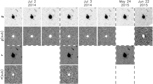
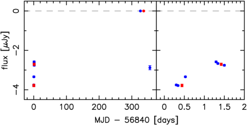
Figure 1: (Top): Original and subtracted images in $g$- and $r$-bands taken with HSC and FOCAS. The field size is $100\times 100$ HSC pixel corresponding to $16.9\times 16.9$ arcsec². North is up and east is left. The image subtraction is done for each image with the HSC image taken on May 24, 2015 being the reference image in the both bands. The original pixel scale of FOCAS is different from that of HSC. We matched the FOCAS data to the HSC data on the WCS basis only for this figure and the pixel scales of the images here are the same. (Bottom): The entire light curves in $g$- and $r$-bands are shown in the left panel in blue and red circles, respectively. The $r$-band photometric point in the reference image (zero flux) in the left panel is shifted by 10 days for readers to see easily. These photometries are done in the subtracted images with references images taken on May 24, 2015. Light curves on Days 1 and 2 are magnified in the right panel.

3.2 Follow-Up Observations with Subaru FOCAS

We took $1200~{}\rm{sec}\times 6$ optical spectra of this object with Faint Object Camera And Spectrograph (FOCAS; Kashikawa et al. (2002)) on the 8.2-m Subaru telescope on June 22, 2015. The slitmask was made for this region and each slit width was 1.0 arcsec. The position angle of the slits was 30 deg and the atmospheric dispersion corrector was used. Seeing was stable and as good as 0.5 arcsec FWHM. We adopted the $2\times 1$ (spatial and dispersion; 0.208 arcsec pixel^-1 and 1.19 Å pixel^-1) binning mode. The first three of the 6 exposures were taken with the VPH850 grism and SO58 order-sort filter (giving $\lambda>5800$ Å spectrum) while the latter three were taken with the 300B grism without any order-sort filters (giving $3500<\lambda<7000$ Å spectrum without 2nd-order contamination). The nominal spectral resolutions were $R\sim 600$ and $\sim 400$ for these two observing modes, respectively. We note that the resulting spectral resolutions ($R\sim 1,200$ and $\sim 800$) were better than these specifications because the image sizes were smaller than the slit widths. Flux calibration was done using the standard star Feige 110 by utilizing the Hubble Space Telescope data (CALSPEC). The data reduction was carrired out first in a standard manner without giving any special attention to the atmospheric absorption feature around 7,580-7,720Å. This is partly because very high-order polynomial fitting is required to correctly evaluate the transmission efficiency in this wavelength range; and, more important, the standard star observation and object observation were done separately in time at a different airmass. It would be more accurate to use simultaneous observational data for the correction, and so we subsequently corrected this absorption feature as described in §4.1.1. The reduced spectra before the correction are shown in the top panel of Figure 2.

We also took $300$-sec $g$-band imaging data in $2\times 2$ binning mode (0.208 arcsec pixel^-1), which enables us to calibrate the flux more accurately. Image subtraction is applied to these FOCAS image after matching the HSC reference image to the FOCAS image because the pixel sampling of FOCAS is larger than that of HSC. Photometry for the data is also shown in Table An Effective Selection Method for Low-Mass Active Black Holes and First Spectroscopic Identification and Figure 1.

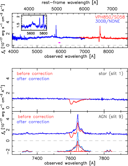
Figure 2: Reduced FOCAS spectra. (top) Entire spectra shown in blue for 300B grism and non-filter and red for VPH850 grism and SO58 filter. AGN Flux density at rest-frame 5100Å estimated from the broad H$\alpha$ luminosity is indicated in magenta. The broad H$\beta$ and [OIII] wavelength region is magnified in the inset. (middle) View around the [OI], H$\alpha$, [NII], and [SII] wavelength region. Spectra without and with atmospheric absorption (red and blue, respectively) for the star used for the correction and the target AGN. Continuum-subtracted spectra and fitted gaussians are shown in light-blue and red, respectively.

4 Measurements of Emission Lines, Black Hole Mass, and Host Galaxy Properties

4.1 Measurements of Emission Line Fluxes and Widths

In the FOCAS spectra, several emission lines are clearly detected and the line identification is secure. However, the H$\alpha$ and [NII] emission line region, which is the most important wavelength region for our purpose, is unfortunately much affected by the strong atmospheric absorption around $7,580$-$7,720$ Å. Therefore, we make a correction for this absorption and evaluate the error it might cause in our measurement of the BH mass.

4.1.1 Atmospheric Absorption Correction

The sky was very clear and stable during the FOCAS observations, which was verified by the CFHT SkyProbe. We consider the sky transmission (absorption) uniform within the 6 arcmin FOCAS field-of-view.

In the slitmask, 1.0 arcsec slits were cut for a few stars as well as for the target AGN. One of the stars in the same slitmask is a G-type star, based on the SDSS color and the FOCAS spectrum, without any strong absorption or emission features around the atmospheric absorption feature. We estimated the absorption fraction by linearly (in the $\lambda$-$f_{\lambda}$ plane) fitting the adjacent continuum of the star spectrum (7550-7580Å and 7750-7800Å) and divided the AGN spectrum by this fraction.

This procedure requires accurate and consistent wavelength calibration between the star and AGN spectra. We examined the positions of the star and AGN in the slits during the exposures. We note that the data was taken at a relatively high elevation and the change of the airmasses during the exposures was not so large, from 1.05 to 1.24. We found the slitmask was well aligned to every object and the difference of the positions to the center of the slits is conservatively evaluated to be smaller than 0.5 pixel, corresponding to 0.6 Å. Then, we iterated the emission line fitting (described in $4.1.2) by shifting the wavelengths of the reference star ($-1.0$ to $+1.0$ pixel; i.e., $-1.2$ Å to $+1.2$ Å) and estimated a systematic error in the measurements of emission line widths and fluxes. We found that the effect of the wavelength difference is smaller than the scatter of the BH mass-to-H$\alpha$ properties and does not affect our result very much. The obtained systematic errors on the broad H$\alpha$ width, luminosity, and BH mass are about 10%, 10%, and 20%, respectively. We note that the systematic error on the final BH mass is smaller than the equation used for calculating the BH mass from the H$\alpha$ properties. We below use the original AGN spectrum without this artificial offset and show only the statistical errors.

4.1.2 Emission Line Measurements

We first fitted one [OI] and two [SII] emission lines after subtracting the surrounding continuum and measured the central wavelengths of the [OI]$\lambda 6300$, [SII]$\lambda 6718$, [SII]$\lambda 6731$ lines as shown in Table An Effective Selection Method for Low-Mass Active Black Holes and First Spectroscopic Identification. The obtained redshift is $z=0.1643$. The measured widths (FWHMs) of the two [SII] lines are consistent with each other and the spectral resolution for the target is $\sim 1,200$. This is also consistent with the fact that the seeing was about 0.5 arcsec FWHM, half of the slit size.

Second, we fitted the continuum of the absorption-corrected spectrum around the H$\alpha$ region with a linear regression line ($\lambda$-$f_{\lambda}$) to isolate the AGN emission lines. After subtracting the continuum, we fitted broad and narrow H$\alpha$ and two [NII] emission lines with four Gaussians simultaneously. In this procedure, we fixed the central wavelengths of the two [NII] components and the narrow H$\alpha$ component, and fixed their widths to be the same as those of the [SII] lines. We also assume the theoretical [NII] line flux ratio of 2.96 (=$f$([NII]$\lambda 6583$)$/f$([NII]$\lambda 6548$). The central wavelengths of the narrow and broad H$\alpha$ are also set to be the same. We finally find that the width and the flux of the broad H$\alpha$ are $1880\pm 120$ km s^-1 and $(61.2\pm 3.1)\times 10^{-17}$ erg s^-1 cm^-2, respectively. All these were similarly done in the previous study (Dong et al., 2012). The emission line properties measured are summarized in Table An Effective Selection Method for Low-Mass Active Black Holes and First Spectroscopic Identification.

In the 300B grism spectrum (3,500-7,000Å), H$\beta$ and [OIII]$\lambda 4959,5007$ lines are significantly detected and H$\beta$ line is in general useful for independent BH mass and extinction measurements. For BH mass measurements, the width of broad H$\beta$ component and the monochromatic continuum luminosity at 5,100Å are required. However, the H$\beta$ broad component is not so strong as H$\alpha$, and the overall spectrum could be contaminated by the host galaxy continuum; moreover, the complex FeII emission and estimation of the continuum flux requires the detailed modeling and fitting of these two components, which is beyond the scope of this paper. Therefore, we here only measure the fluxes of these emission lines (Table An Effective Selection Method for Low-Mass Active Black Holes and First Spectroscopic Identification) by summing the flux instead of fitting the lines to derive the flux ratio $f(\rm{[OIII]})/f(\rm{H}\beta)$.

UV-optical variability is detected from this AGN and the clear broad H$\alpha$ and H$\beta$ emission lines are also detected. These facts indicate that the AGN UV-optical emission from the accretion disk does not suffer from heavy extinction. However, we here estimate possible extinction originated from dust in the host galaxy with the Balmer decrement method. As stated in the above paragraph, the narrow H$\beta$ emission line is not clearly detected and the rough lower limit of the flux ratio $f(H\alpha)/f(H\beta)>5$ for the narrow components is obtained. This flux ratio is larger than that expected in the Case B recombination and that of the broad components of this object ($\sim 3.6$) which is only slightly larger than the median value of 3.06 for type-1 AGN (Dong et al., 2008). Assuming the Calzetti extinction law (Calzetti et al., 2000), we estimated dust extinction of $A(H\alpha,narrow)\gtrsim 1.4$ mag (a factor of $\gtrsim 3.5$) and $A(H\alpha,broad)\sim 0.6$ mag (a factor of $\sim 1.7$) at the H$\alpha$ wavelength, which corresponds to a possible BH mass underestimation by a factor of $\gtrsim 1.9$ and $\sim 1.3$, for the narrow and broad components, respectively.

4.1.3 Black Hole Mass Measurements

H$\alpha$ width (FWHM) and luminosity are often used for estimating BH masses, especially for low-mass BHs (Greene & Ho (2005); Dong et al. (2012); Schramm et al. (2013)). We convert the broad H$\alpha$ luminosity and width to estimate the BH mass by an equation (A1) in Greene & Ho (2007b), $M_{\rm{BH}}=(3.0^{+0.6}_{-0.5})\times 10^{6}\left(L_{\rm{H\alpha}}/10^{42}~{}\rm{~{}[erg~{}s}^{-1}\rm{]}\right)^{0.45\pm 0.03}\\ \left(\rm{FWHM_{H\alpha}}/10^{3}\rm{~{}[km~{}s}^{-1}]\right)^{2.06\pm 0.06}~{}\rm{[M}_{\odot}\rm{]}$. The obtained BH mass is $M_{\rm{BH}}=(2.7\pm 0.6)\times 10^{6}$ [M_⊙].

Monochromatic luminosity at 5100Å, $\lambda L_{\lambda}(5100$Å), and bolometric luminosity $\lambda L_{\rm{bol}}$ can be evaluated by equations in Greene & Ho (2005), $\lambda L_{\lambda}(5100\rm{\AA})=10^{44}\left(L_{\rm{H\alpha}}/5.25\times 10^{42}~{}\rm{[ergs}^{-1}\rm{]}\right)^{(1/1.157)}~{}\rm{[erg~{}s}^{-1}~{}\rm{]}$ and $L_{\rm{bol}}=\lambda L_{\lambda}(5100\rm{\AA})\times c_{\rm{bol}}~{}\rm{[erg~{}s}^{-1}~{}\rm{]}$. The flux density at the rest-frame 5,100Å  is found to be $4.4\times 10^{-18}$ [erg s^-1 cm^-2 Å^-1] and this indicates that luminosity fraction of AGN relative to the total luminosity, $L_{\lambda}(\rm{5100\AA}$; AGN)$/L_{\lambda}(\rm{5100\AA}$; AGN$+$galaxy), is 0.33 as shown in the top panel of Figure 2.

Based on the BH mass and H$\alpha$ luminosity, we calculate the Eddington ratio to be 0.046 by assuming a bolometric correction of $c_{\rm{bol}}=9.8$ (McLure & Dunlop, 2004). We locate our object in figures of apparent $g$-band total magnitude, apparent $g-r$ color without deblending, broad H$\alpha$ width (FWHM), H$\alpha$ luminosity, BH mass, and Eddington ratio, as a function of redshift by comparing with the sample in Dong et al. (2012) (Figure 3).

A major limitation of the SDSS studies is the detection of broad H$\alpha$ emission lines, which roughly corresponds to a limit on the flux of broad H$\alpha$ lines, $f(\rm{H}\alpha)\geq 5.2\times 10^{-16}$ [erg s^-1 cm^-2] (Dong et al., 2012). This can be converted to the limits of luminosity and width of H$\alpha$ ($L(\rm{H}\alpha$) and FWHM(H$\alpha$)), bolometric luminosity ($L_{\rm{bol}}$), and Eddington ratio ($L_{\rm{Edd}}/L_{\rm{bol}}$) given the definition (upper limit) of the BH masses of $2\times 10^{6}$ M_⊙. These limits are shown in gray lines in Figure 3. Our object has a slightly higher BH mass compared to the SDSS studies and is close to the lower-end of the H$\alpha$ luminosity distribution, resulting in lower Eddington ratio, thanks to its apparent faintness relative to other galaxies in the same redshift range.

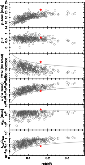
Figure 3: Apparent $g$-band magnitude, apparent $g-r$ color without deblending, FWHM and luminosity of broad H$\alpha$ emission line, BH mass, and Eddington ratio as a function of redshift of our target AGN (red star) and low-mass active BHs in Dong et al. (2012) (black circle). The limits of the SDSS study (Dong et al., 2012) are shown in gray lines.

Figure 4 is a BPT diagram for our target and objects in Dong et al. (2012). We note again that the [OI] and [SII] emission lines can be more securely measured than the [NII] emission lines. We locate two points for our object in each panel. We also note that the flux of the H$\beta$ emission line is measured for the entire H$\beta$ emission line dominated by the broad component. As shown in similar studies (e.g., Schramm et al. (2013)), the location of our object indicates these elements are dominantly excited by star forming activity rather than the AGN activity, or a composite of star forming and low-ionization narrow emission-line regions (LINER)-like activities, if one tries to classify objects without deblending emission lines into narrow and broad components. This indicates that measurements of emission line ratios do not work for selecting our object. On the other hand, two-thirds of the objects in the sample of Dong et al. (2012) are located at the Seyfert regions as shown in Figure 4.

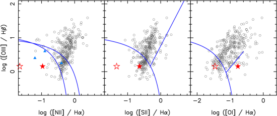
Figure 4: BPT diagram for our target (red open stars for broad and narrow components of H$\alpha$ and filled stars for only narrow H$\alpha$ emission lines) and objects in Dong et al. (2012) (black circles) and Schramm et al. (2013) (only in the left panel, blue triangles). Lines separating HII region, LINER, and Seyfert nuclei derived from Kewley et al. (2006) are shown.

4.2 Host Galaxy Properties

We measure the radial profile of the host galaxy with GALFIT (Peng et al., 2010). The fitting was done for the HSC images in all the epochs in $g$- and $r$-bands with masks covering a northern star, an eastern star, and an east-south extended source, close to the target. We note that the emission line contributions are small according to the spectra (Figure 2). We fit the images with a PSF at the position of the AGN (galaxy center) and an extended component with a Sérsic profile of Sérsic index $n$ (Sérsic, 1963).

The fitting results are all well done (reduced $\chi^{2}\sim 1$) and nicely consistent in all the epochs. A half-light radius is $r_{e}=3.5-4.0$ pixel ($\sim 2$ kpc) and Sérsic index is $n=0.5-1.0$ with measurement errors of about 0.5 pixel and 0.1, respectively. The $g$- and $r$-band magnitudes of the Sérsic (extended) component are $21.6\pm 0.2$ mag and $20.7\pm 0.1$ mag, respectively, giving $g-r$ color of about 0.9. The axis ratios and the position angles are $0.80\pm 0.05$ and $15\pm 10$ degrees, respectively.

The morphological information indicates that the host galaxy is a disk galaxy. Based on a recent study on galaxy morphologies by Lange et al. (2015), the Sérsic index and size of the galaxy indicate that the host galaxy stellar mass is about $10^{9}$ M_⊙ although the intrinsic scatter is large. This stellar mass is within the scatter of the BH-to-total mass ratio for $2.7\times 10^{6}$ M_⊙ objects shown in Reines et al. (2015). In the previous SDSS studies (Greene & Ho (2007a); Dong et al. (2012)), although it is difficult to examine the morphology of the host galaxies with the image quality of the SDSS data, the measured $g-r$ colors of the host galaxies are somewhat red but still consistent with colors of disk galaxies. (Greene & Ho (2007a); Dong et al. (2012)). The $g-r$ color of the host galaxy of our object is redder than the median values in those papers but still within the range of their $g-r$ colors.

5 Discussion & Summary

We selected a low-mass active BH candidate through short-time scale variability selection based on 1-hour-cadence imaging data with Subaru HSC, and spectroscopically determined that the object hosts an active BH, the mass of which we find to be $2.7\times 10^{6}$ M_⊙ based on the H$\alpha$ emission line after careful correction of the spectrum. This object is located at a relatively low redshift, within the redshift range probed by the SDSS dataset (Greene & Ho (2005); Dong et al. (2012)). Our object is relatively bright in our HSC data and almost at the faint-end limit of the SDSS data. Compared with the SDSS samples, the H$\alpha$ width is broader and the H$\alpha$ luminosity is as small as those of the faintest SDSS objects as shown in Figure 3. The obtained BH mass is slightly above the upper end of those two previous studies (because of their mass criteria for low-mass BHs).

Our method is observationally limited solely by variability detection. If we assume that variability amplitude is constant over wide ranges of BH mass and Eddington ratio, variability amplitude is expected to be proportional to AGN luminosity, which is the product of BH mass and Eddington ratio, as described in equation 5, where $f_{\rm{vari}}$ and $c_{\rm{bol}}$ are variability amplitude and bolometric correction, respectively.

$$\Delta{L} = f_{\rm{vari}}\times\frac{1}{c_{\rm{bol}}}\times\frac{L_{\rm{bol}}}{L_{\rm{Edd}}}\times\left(1.26\times 10^{38}(M/M_{\odot})\right)~{}\rm{[erg~{}s}^{-1}\rm{]}$$

$${\rm where}\quad L_{\rm{Edd}}=4\pi Gcm_{p}M/\sigma_{e}=1.26\times 10^{38}(M/M_{\odot})~{}\rm{[erg~{}s}^{-1}\rm{]}$$

By roughly assuming $f_{\rm{vari}}=0.1$ (10%) (Vanden Berk et al., 2004), variability amplitude defined as magnitude of differential flux in subtracted images can be calculated as a function of redshift. For a low-mass active BH at $z=0.164$, the total flux including the host galaxy component is about 15 $\mu$Jy and the AGN component is a third of the total flux: about 5 $\mu$Jy. The variability amplitude from hours to a day is about 10%, while that at time scales longer than a day is larger than 20%. We here assume that the power-law index of AGN spectra ($f_{\nu}\propto\nu^{\alpha_{\nu}}$) is $\alpha_{\nu}=-0.44$ (Vanden Berk et al., 2001). We also assume $g$-band HSC observations with a typical depth in a 10 minute exposure of $g\sim 26$ mag. In this case, variability detection can go down to $g_{\rm{vari}}\sim 25.6$ mag, which is shallower than the original images by a factor of $\sqrt{2}$. This is because we need to investigate intranight variability, not variability relative to deep reference images. Under these assumptions, we can calculate the BH mass range from which we can detect variability as shown in Figure 5.

In the SDSS studies, the optical wavelength range and depths ($r<17.77$ for the spectroscopic sample described in Strauss et al. (2002) and $r\sim 20$ for some deeper specific samples) limit the redshift ($z<0.352$ for H$\alpha$; Greene & Ho (2007b); Dong et al. (2012)) and brightness ranges. Figure 5 indicates that our variability survey can find smaller active BHs at higher redshifts than the SDSS although AGN variability amplitude is not so large that it is more difficult to detect the variability than the objects themselves. The Prime Focus Spectrograph (PFS; Takada et al. (2014)), to be attached to the 8.2-m Subaru telescope in near future, will achieve a wider wavelength coverage, up to $J$-band, 1.26 $\mu$m, corresponding to the limit of H$\alpha$ detection at $z\sim 0.85$, and deeper spectroscopic capability. Compared to these two large spectroscopic surveys, which naively require blind galaxy spectroscopic observations, our selection based on multi-epoch imaging data over one or a few nights is less expensive. Since in the blind spectroscopic SDSS surveys, the low-mass active BH ($<2\times 10^{6}$ M_⊙) fraction is as small as 0.03% ($174/544,127$; Greene & Ho (2007a); Greene & Ho (2007b)) and 0.07% (309/451,000; Dong et al. (2012)), our HSC survey has the advantage of effectively selecting low-mass active BH candidates as spectroscopic targets. For example, given these low success rates of the blind spectroscopic surveys and the number of fibers of PFS (2,400), one fiber is accidentally assigned to a low-mass active BH on average but the expected number density of these populations is larger based on the number density shown in the previous SDSS study (Greene & Ho, 2007b). In our current dataset, we have photometrically detected short timescale variability from an order of ten candidates per HSC field-of-view, whose nature should be examined with spectroscopic data.

The sample size will be enhanced by larger HSC surveys and coming LSST survey. Low-mass active BH candidates selected based on our method will be good candidates for systematic spectroscopic observations with PFS. This variability method basically has no redshift limitation except for the effect of Lyman break and brightness, although AGN identification and BH mass measurements in spectroscopic observations with current facilities might limit the capability of our method. This will be improved in the era of 30-m class telescopes.

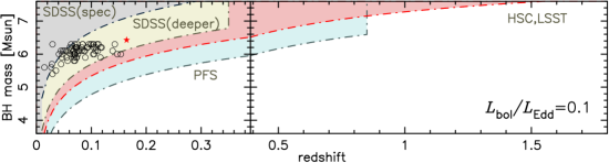
Figure 5: Detectable BH mass as a function of redshift. Eddington ratio ($L_{\rm{bol}}/L_{\rm{Edd}}$) of 0.1 is assumed. Variability amplitude of 10% ($f_{\rm{vari}}=0.1$) is also assumed. Our target AGN is shown as a red star and the SDSS objects with $L_{\rm{bol}}/L_{\rm{Edd}}\sim 0.1$ are plotted in open circles.

This research was partially supported by JSPS Grants-in-Aid for Scientific Research (15H05440, 25800103, 15H02075, 23224004, and 26400222), the Toyota Foundation (D11-R-0830), and the World Premier International Research Center Initiative, MEXT, Japan. The work of SB is supported by the RF grant 11.G34.31.0047. This paper is based in part on data collected at Subaru Telescope, which is operated by the National Astronomical Observatory of Japan. This paper makes use of software developed for the Large Synoptic Survey Telescope. We thank the LSST Project for making their code available as free software at http://dm.lsstcorp.org. We also appreciate a kind help by Prof. Michael W. Richmond for improving the English grammar of the manuscript.

Light Curves Relative to the Reference Images Taken on May 24, 2015. date MJD Day Inst filter $t_{\rm{exp}}$ flux(sub) mag(sub) seeing [sec] [$\mu$Jy] [mag] [arcsec] 2014-07-02 56840.299 1 HSC $g$ 600 $-3.756\pm 0.036$ $22.46^{+0.01}_{-0.01}$ 0.54 2014-07-02 56840.342 1 HSC $g$ 600 $-3.787\pm 0.029$ $22.45^{+0.01}_{-0.01}$ 0.75 2014-07-02 56840.526 1 HSC $g$ 600 $-3.343\pm 0.036$ $22.59^{+0.01}_{-0.01}$ 1.19 2014-07-03 56841.293 2 HSC $g$ 600 $-2.583\pm 0.040$ $22.87^{+0.02}_{-0.02}$ 0.71 2014-07-03 56841.338 2 HSC $g$ 600 $-2.668\pm 0.033$ $22.83^{+0.01}_{-0.01}$ 0.70 2014-07-03 56841.500 2 HSC $g$ 600 $-2.756\pm 0.037$ $22.80^{+0.01}_{-0.01}$ 0.79 2015-05-24 57166.467 327 HSC $g$ 1080 $0$ - 0.62 2015-06-22 57195.387 356 FOCAS $g$ 300 $-2.881\pm 0.103$ $22.75^{+0.04}_{-0.04}$ 0.61 2014-07-02 56840.442 1 HSC $r$ 600 $-3.782\pm 0.064$ $22.46^{+0.02}_{-0.02}$ 0.72 2014-07-03 56841.422 2 HSC $r$ 600 $-2.708\pm 0.059$ $22.82^{+0.02}_{-0.02}$ 0.49 2015-05-24 57166.398 327 HSC $r$ 360 $0$ - 0.68

Emission Line Properties. Line $\lambda_{\rm{cen}}$ [Å] Width [Å] Flux [$10^{-17}$ erg s^-1 cm^-2] $[$SII$]$$\lambda 6731$ $7819.99$ $7.69\pm 1.72$ $1.70\pm 0.33$ $[$SII$]$$\lambda 6718$ $7836.76$ $5.55\pm 0.78$ $1.88\pm 0.27$ $[$NII$]$$\lambda 6584$ – – $0.19\pm 0.82$ H$\alpha$ (narrow) – – $15.69\pm 0.95$ H$\alpha$ (broad) – $47.95\pm 2.97$ $61.16\pm 3.13$ $[$NII$]$$\lambda 6548$ – – $0.57\pm 0.28$ $[$OI$]$$\lambda 6300$ $7338.93$ $11.72\pm 1.92$ $2.68\pm 0.40$ $[$OIII$]$$\lambda 5007$ – – $11.92\pm 2.26$ $[$OIII$]$$\lambda 4959$ – – $4.00\pm 0.76$ H$\beta$ – – $17.16\pm 0.93$ We show only fitted parameters. The redshift determined by the [OI] and [SII] emission line wavelengths.

References

- Aihara et al. (2011) Aihara, H., et al. 2011, ApJS, 195, 26
- Ajello et al. (2012) Ajello, M., et al. 2012, ApJ, 751, 68
- Alard & Lupton (1998) Alard, C., & Lupton, R. H. 1998, ApJ, 503, 325
- Alard (2000) Alard, C. 2000, A&AS, 144, 363
- Axelrod et al. (2010) Axelrod, T., et al. 2010, SPIE, 7740, 15
- Baldassare et al. (2015) Baldassare, V., et al. 2015, ApJ, 809, 14
- Barth et al. (2004) Barth, A. J., Ho, L. C., Rutledge, R. E., & Sargent, W. L. W. 2004, ApJ, 607, 90
- Barth et al. (2014) Barth, A. J., et al. 2014, AJ, 147, 12
- Bauer et al. (2009) Bauer, A., et al. 2009, ApJ, 705, 46
- Calzetti et al. (2000) Calzetti, D., Armus, L., Bohlin, R. C., Kinney, A. L., Koornneef, J., & Storchi-Bergmann, T. 2000, ApJ, 533, 682
- Choi et al. (2014) Choi, Y., et al. 2014, ApJ, 782, 37
- Cohen et al. (2006) Cohen, S. H., et al. 2006, ApJ, 639, 731
- Croom et al. (2004) Croom S. M., Smith R. J., Boyle B. J., Shanks T., Miller L., Outram P. J., Loaring N. S., 2004, MNRAS, 349, 1397
- de Vries et al. (2005) de Vries, W. H., Becker, R. H., White, R. L., & Loomis, C. 2005, AJ, 129, 615
- Dong et al. (2008) Dong, X., Wang, T., Wang, J., et al. 2008, MNRAS, 383, 581
- Dong et al. (2012) Dong, X.-B., et al. 2012, ApJ, 755, 167
- Furusawa et al. (2010) Furusawa, H., et al. 2010, SPIE, 7740, 2IF
- Furusawa et al. (2011) Furusawa, H., et al. 2011, PASJ, 63, 585
- Furusawa et al. (2015) Furusawa, H., et al. 2016, in prep.
- Hawkins & Veron (1993) Hawkins, M. R. S., & Veron, P., 1993, MNRAS, 260, 202
- Greene & Ho (2004) Greene, J.E., & Ho, L. C., 2004, ApJ, 610, 722
- Greene & Ho (2005) Greene, J.E., & Ho, L. C., 2005, ApJ, 630, 122
- Greene & Ho (2007a) Greene, J.E., & Ho, L. C., 2007 ApJ, 667, 131
- Greene & Ho (2007b) Greene, J.E., & Ho, L. C., 2007 ApJ, 670, 92
- Ivezic et al. (2008) Ivezic, Z., et al. 2008, arXiv0805.2366I
- Kashikawa et al. (2002) Kashikawa, N., et al. 2002, PASJ, 54, 819
- Kewley et al. (2006) Kewley, L. J., et al. 2006, MNRAS, 372, 961
- Komatsu et al. (2009) Komatsu, E., Dunkley, J., Nolta, M. R., et al. 2009, ApJS, 180, 330
- Kranz et al. (2010) Kranz, W. D., Tran, K.-V., Giordano, L., & Saintonge, A., ApJ, 140, 561
- Lange et al. (2015) Lange, R., et al. 2015, MNRAS, 447, 2603
- McLure & Dunlop (2004) McLure, R. J., & Dunlop, J. S. 2004, MNRAS, 352, 1390
- Miyazaki et al. (2010) Miyazaki, S., et al. 2012, SPIE, 8446E, 0ZM
- Mortlock et al. (2011) Mortlock, D. J., et al. 2011, Nature, 474, 7353, 619
- Lehmer et al. (2005) Lehmer, B. D., et al. 2005, ApJS, 161, 21
- Morokuma et al. (2008a) Morokuma, T., et al. 2008a, ApJ, 676, 121
- Morokuma et al. (2008b) Morokuma, T., et al. 2008b, ApJ, 676, 163
- Peng et al. (2010) Peng et al. 2010, AJ, 139, 2097
- Peterson et al. (2005) Peterson, B. M., et al. 2005, ApJ, 632, 799
- Reines et al. (2011) Reines, A. E., Sivakoff, G. R., Johnson, K. E., & Brogan, C. L. 2011, Nature, 470, 66
- Reines & Deller (2012) Reines, A. E., & Deller, A. T. 2012, ApJ, 750, 24
- Reines et al. (2013) Reines, A. E., et al. 2013, ApJ, 775, 116
- Reines et al. (2015) Reines, A. E., & Volonteri, M., 2015, ApJ, 813, 82
- Ruan et al. (2012) Ruan, J. J., et al. 2012, ApJ, 760, 51
- Sarajedini et al. (2006) Sarajedini, V., et al. 2006, ApJS, 166, 69
- Schramm et al. (2013) Schramm, M., et al. 2013, ApJ, 773, 150
- Schlafly & Finkbeiner (2011) Schlafly, E. F. & Finkbeiner, D. P., 2011, ApJ, 737, 103
- Sérsic (1963) Sérsic J. L., 1963, Bol. Asociacion Argentina Astron., 6, 41
- Shen et al. (2011) Shen, et al. 2011, ApJS, 194, 45
- Strauss et al. (2002) Strauss, M. A., et al. 2002, AJ, 124, 1810
- Takada et al. (2014) Takada, M., et al. 2014, PASJ, 66, 1
- Tanaka et al. (2014) Tanaka, M., et al. 2014, ApJ, 793, 26
- Tanaka et al. (2016) Tanaka, M., et al. 2016, ApJ in press. (arXiv:1601.03261)
- Tominaga et al. (2011) Tominaga, N., et al. 2011, ApJS, 193, 20
- Tominaga et al. (2014a) Tominaga, N., et al. 2014a, ATel, 6291, 1
- Tominaga et al. (2014b) Tominaga, N., et al. 2014b, ATel, 6763, 1
- Tominaga et al. (2015a) Tominaga, N., et al. 2015a, ATel, 7565, 1
- Tominaga et al. (2015b) Tominaga, N., et al. 2015b, ATel, 7927, 1
- Tominaga et al. (2015c) Tominaga, N., et al. 2016, submitted to ApJ
- Vanden Berk et al. (2001) Vanden Berk, D., et al. 2001, AJ, 122, 549
- Vanden Berk et al. (2004) Vanden Berk, D., et al. 2004, ApJ, 601, 692
- White et al. (1997) White, R. L., Becker, R. H., Helfand, D. J., & Gregg, M. D. 1997, ApJ, 475, 479
- Xue et al. (2011) Xue, Y. Q., et al. 2011, ApJS, 195, 10
- York et al. (2000) York, D. G., Adelman, J., Anderson, J. E., Jr., et al. 2000, AJ, 120, 1579