Detecting Topological Order with Ribbon Operators
Abstract
We introduce a numerical method for identifying topological order in two-dimensional models based on one-dimensional bulk operators. The idea is to identify approximate symmetries supported on thin strips through the bulk that behave as string operators associated to an anyon model. We can express these ribbon operators in matrix product form and define a cost function that allows us to efficiently optimize over this ansatz class. We test this method on spin models with abelian topological order by finding ribbon operators for quantum double models with local fields and Ising-like terms. In addition, we identify ribbons in the abelian phase of Kitaev’s honeycomb model which serve as the logical operators of the encoded qubit for the quantum error-correcting code. We further identify the topologically encoded qubit in the quantum compass model, and show that despite this qubit, the model does not support topological order. Finally, we discuss how the method supports generalizations for detecting nonabelian topological order.
Despite the apparent simplicity of quantum spin models, they can exhibit a wide variety of interesting and potentially useful phenomena. These range from conventional magnetic order to the more novel topologicalWen (2013) and symmetry-protectedChen et al. (2013) and symmetry-enrichedBarkeshli et al. (2014) topological orders which are of interest in both condensed matter physicsAnderson (1987) and quantum information theory.Kitaev (2003) These states are disordered in the sense of Landau-Ginzburg-Wilson, however they do exhibit properties distinct from the usual disordered phases. For example, topological phases possess quasiparticle excitations, known as anyons, whose braid relations can be far more exotic than those of fermions or bosons.Nayak et al. (2008) These phases also have ground state degeneracy which depends on the topology of the lattice.Wen and Niu (1990) This protected degeneracy has prompted the investigation of topologically ordered models as quantum memories.Kitaev (2003); Dennis et al. (2002) Quantum information stored in the degenerate subspace can be protected from arbitrary local noise when error correction techniques are employed.Brown et al. (2014); Terhal (2015); Brell et al. (2014)
Distinguishing topological phases can be an especially challenging task precisely because of their topological nature: there is no broken symmetry and no local order parameter signalling the phase transition.Wen (2013) There has been a large amount of previous work which attempts to identify topological order (TO). The existing key techniques, such as the topological entanglement entropy,Levin and Wen (2006); Kitaev and Preskill (2006); Flammia et al. (2009); Isakov et al. (2011); Zhang et al. (2012); Jiang et al. (2012) the entanglement HamiltonianLi and Haldane (2008), topological degeneracyTrebst et al. (2007) and associated properties,Zhang et al. (2012); Cincio and Vidal (2013) symmetries of particular representations of the ground states,Schuch et al. (2010); Buerschaper (2014); Şahinoğlu et al. (2014); Bultinck et al. (2015); Liu and Wen (2015) and specific properties of particular TO states,Evenbly and Vidal (2010); Yan et al. (2011) have been highly successful in various domains of applicability. We review these methods below. A common feature of these methods is that they utilize the ground state of the model, which is unfortunately a challenging computational task in general.
Here we propose a numerical method that we call the ribbon operators method for identifying TO in the ground state of a given 2D Hamiltonian using only the Hamiltonian, without reference to the ground state. We reduce the search for TO to a 1D problem through the bulk of the material, and we present a variational approach based on standard DMRGSchollwöck (2011) to identify certain operators – the ribbon operators – supported in the bulk that satisfy the commutation relations relevant for a candidate anyon model. We demonstrate the power of this approach by identifying TO in both integrable and non-integrable models, and contrast this with topologically trivial Hamiltonians. We also demonstrate the ability to identify topologically encoded qubits and logical operators of quantum error-correcting codes, even in a non-integrable model. All of our calculations are focused on the case of abelian TO in spin models, however the ribbon operators method suggests several natural extensions beyond this case, which we leave open for future work.
The following subsection reviews prior approaches, while Sec. I reviews anyon models. The expert reader can skip to Sec. II.
.1 Prior Approaches
One important tool is the topological entanglement entropy (TEE)Levin and Wen (2006); Kitaev and Preskill (2006) of the ground state wave function. Given the reduced density matrix of some many-body ground state on a region , the von Neumann entropy typically obeys the area law
| (1) |
where and are the number of spins in the region and on the boundary of the region respectively, and is the TEE.
In a topologically ordered model, a physical argument suggests that , where is the quantum dimension of the anyon with charge in the associated anyon model. The TEE is clearly nonzero if the ground state is topologically ordered,Levin and Wen (2006) so can be used as a signal of such ordering.Isakov et al. (2011); Zhang et al. (2012); Jiang et al. (2012) One can compute by obtaining an explicit ground state wavefunction, for example as a PEPS. Additionally, a Rényi entropy variant of Flammia et al. (2009) can be computed by sampling the ground state wavefunctions using quantum Monte Carlo.Isakov et al. (2011)
There are two major challenges associated with this approach. Firstly, there exist examples of topologically trivial states for which computing leads to nonzero values.Zou et al. Secondly, any two topological phases whose associated anyon models have the same total quantum dimension will have the same TEE, and so it cannot be used to distinguish them. This second problem has already led to difficulty in fully identifying the phase of physically interesting models including the Heisenberg antiferromagnet on the Kagome lattice, a model thought to describe the low-energy physics of several naturally occurring and synthetic minerals.Jiang et al. (2012)
A less coarse approach is to investigate the full entanglement spectrum, that is, the spectrum of the effective Hamiltonian defined by .Li and Haldane (2008) It has been suggested that the universal properties of are intimately linked to the structure of the physical edge state of the model, however can undergo phase transitions without the physical model doing so,Chandran et al. (2014) and at least for models in the same phase as a string-net modelLevin and Wen (2005) the spectrum is expected to contain the same universal information as the TEE.Flammia et al. (2009)
One of the characteristic features of topologically ordered models is the topology-dependent ground state degeneracy.Wen and Niu (1990) After obtaining a full set of ground states, one can observe transitions out of topological phases via loss of topological degeneracy,Trebst et al. (2007) and, in the topological phase, compute the and matrices defining the braiding relations in the associated anyon theory.Zhang et al. (2012); Cincio and Vidal (2013) Unfortunately, demonstrating topology-dependent ground state degeneracy is not sufficient to ensure robust topological order.Nussinov and Ortiz (2009, )
Given a projected entangled pair state (PEPS) description of the ground state, one can identify the topological order by understanding the symmetry properties of the parent HamiltonianSchuch et al. (2010) or the environment tensor.Liu and Wen (2015) One can also use the PEPS formalism to identify matrix product operators (MPOs) that ‘pull through’ the PEPS tensors on the virtual level.Şahinoğlu et al. (2014); Bultinck et al. (2015) These MPOs are in close analogy to the physical operators that act to create and transport anyons. As we will describe, these physical operators are central to our approach.
Finally, given access to a ground state, specific structure such as certain correlation functions or distribution of bond energies can provide evidence for topological ordering.Evenbly and Vidal (2010); Yan et al. (2011)
As a prerequisite for each of these methods, one must obtain an efficient description of the ground space (e.g. via tensor networks) or obtain expectations with respect to ground states (e.g. via Monte Carlo sampling). Tensor network (TN) methods have proven very useful for this purpose,Jiang et al. (2012); Cirac et al. (2011); Yan et al. (2011); Evenbly and Vidal (2010); Liu and Wen (2015) however in many cases the result does not conclusively determine the topological order.Yan et al. (2011) The TN states obtained suffer from several drawbacks. In particular, they are usually computed on infinite cylinders of small circumference. They can also be biased towards low-entanglement states.Evenbly and Vidal (2010) Additionally, properties of a ground state alone are not sufficient to identify a gapped topological phase. For example, a one can obtain a gapless Hamiltonian sharing the toric code ground space.Freedman et al. (2008)
Of these methods, the ones closest in spirit to our current approach are the tensor network-based methods,Schuch et al. (2010); Şahinoğlu et al. (2014); Bultinck et al. (2015) however our approach differs substantially in that we do not require a PEPS description of the ground state wavefunction. We instead variationally create tensor network representations of certain ribbon operators that are supported on 1D strips through the truly two-dimensional bulk; this dimensional reduction is what makes our method numerically tractable. In contrast to state-based variational approaches, where a similar reduction is often included for numerical convenience, we will argue that in our operator-based approach this reduction is an expected feature of the operators. Additionally, if one wishes to use the topologically protected ground space as a quantum memory, knowledge of these ribbon operators is required for information manipulation and extraction. Thus, this method could be used to augment a state-based approach to obtain this additional data.
This paper is organized as follows. In Sec. I, we review some of the features of anyon models which describe the low energy excitations of topologically ordered spin models. In Sec. II, we define a ribbon operator, and use the properties of the anyons to define a cost function which quantifies how well a candidate ribbon realizes their behavior. We then describe how the cost function can be minimized numerically in Sec. IV. Using this algorithm, in Sec. V we obtain ribbon operators in a number of topologically ordered and topologically trivial models. These numerics demonstrate that the cost function we define allows identification of abelian topological order in nonintegrable spin models. In Sec. VI, we prove that, under certain assumptions, ribbon operators can be used as approximate logical operators in quantum error correcting codes. We conclude in Sec. VII with a discussion of extensions of the method to nonabelian topological order and more complex spin models.
I Properties of Anyons
In this section, we review the physical properties of anyon models that characterize a topological phase. Of course, not all topological phases have an associated anyon model, for example the cubic code,Haah (2011) however we will tailor our method to those phases with anyonic excitations. This discussion of anyon models will motivate our definition in the subsequent section of a ribbon operator for a spin model defined by some local Hamiltonian on a lattice in two dimensions. We will argue that this definition captures the essential features outlined below of a topologically ordered model by thinking about anyons as quasiparticle excitations of the spin model. The simplest realization of this is Kitaev’s toric code,Kitaev (2003, 2006) and we will refer to that model to clarify key features.
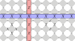
Creating a pair of anyons, and moving them to the boundary of the lattice leaves no excitations, and so maps the vacuum to the vacuum. In the toric code, anyons are created and transported using string operators, as shown in Fig. 1. These operators commute with the Hamiltonian in the bulk, but have excitations localized to the ends. In this way, if the anyons are moved off the edge of the lattice or are fused together, the system remains in its ground state.
More generally, we expect anyonic excitations to be particle like, but to have nontrivial braiding relations. On sufficiently large length scales, it is expected that these braid statistics are governed solely by an anyon model.Kitaev (2006) For this reason, the creation operators in this limit should be one dimensional with the particles localized around the end points. Away from a renormalization-group fixed point, we expect these operators to be dressed, and supported on slightly fattened regions, though still effectively one-dimensional. More precisely, the width of these ribbons should be set by the microscopic details of the model, and should not scale with system size.
The family of local commuting projector codes (LCPC) generalizes the toric code and provides a concrete instantiation of these ideas. The LCPCs are families of Hamiltonians where the terms are pairwise commuting projectors onto an unfrustrated ground state. In these models the string operators described above always exist.Haah and Preskill (2012) This class of models includes exactly solvable points of most known topological phasesLandon-Cardinal and Poulin (2013) including the Levin-Wen string nets.Levin and Wen (2005) Away from these exactly solvable points, we can dress the string operators using quasiadiabatic continuation.Hastings and Wen (2005) Given a point in a phase for which an initial string operator exists, such as an LCPC, we can dress this operator to any other point in the phase. Generically this operator will have extensive support, however the error made in truncating the width is exponentially small in , where is the width and is the correlation length. Thus string-like operators with width proportional to the correlation length can be found anywhere within the phase.
Since the string operators act as creation operators for pairs of anyons, we argue that they should be only slightly entangling operators.Haah and Preskill (2012) These are operators whose Schmidt rank is independent of the system size on any bipartition that cuts the string into two contiguous pieces. In the LCPC case, the string operators are known to be slightly entangling.Haah and Preskill (2012) Since the quasiparticles are simply dressed by moving away from these fixed points, we expect this property to remain throughout the phase; although the required Schmidt rank can increase substantially, it will still be independent of the system size. When we remove the dressed quasiparticles from the lattice (by annihilating them or bringing them out to infinity), the system returns to its ground space, which is expected to obey the area law of Eq. (1). This also supports the slightly entangling nature of such operators.
Some of the defining features of an anyon model are the relations that are encoded in the topological matrix and the matrices. Let label the anyonic particles in the anyon model describing the low energy excitations of the Hamiltonian . The matrices are defined by
| (3) |
and the matrix is
| (5) |
where the lines trace out the worldlines of the particles.
Another approach is to consider the related matrix that can be obtained via the twist product.Haah (2016) If the matrix is an object that captures dynamical information from braiding anyons in 2+1 dimensions, then the matrix is a static object that captures correlations of ground states in 2+0 dimensions. If is an operator supported on an annulus that projects onto a state with total charge inside, then
| (6) |
where is any ground state of the spin model. For bipartite operators and , the twist product with respect to the partition is defined as
| (7) |
where the order is reversed on the region relative to the partition. This is clearly closely related to Eq. (5), where the worldline loops are replaced by the corresponding closed loop operators on the lattice. For abelian models where for all particle types , the and matrices coincide up to a multiple of .
Finally, anyonic quasiparticles should be able to move around the lattice, and the state should not depend upon any smooth deformations of the path they take. In particular, when they are fused back together or moved off the lattice, the system should return to a vacuum state. This is realized in the toric code since the string operators can be deformed by dressing with local operators that are symmetries of the Hamiltonian. This preserves commutativity with and the matrix and clearly creates the same particle at the ends.
II Definition of Ribbon Operators
Let us summarize the physical intuition that we’ve gained in the previous section into a few simple properties that the string-like operators seem to possess in general. These properties hold for known exactly solvable models with TO.
Given a two-dimensional quantum system with TO, we expect that there are operators supported on one-dimensional strips through the bulk where the following four properties hold, at least approximately:
-
1.
commutes with the bulk Hamiltonian in the low energy sector.
-
2.
is supported on a strip of spins with bounded width .
-
3.
Distinct ribbons and should respect the data (e.g. the or matrix) for an underlying anyon model in the low energy sector.
- 4.
Since finding a low energy projector appears to be a challenging task, we make the following assumption. Rather than asking for 1-4 to hold only in the low energy sector, we ask for them to hold on the whole spectrum. At first glance, this seems to be too strong for characterizing TO away from an exactly solvable RG fixed point. Nonetheless, by making this assumption, we can arrive at an effective numerical procedure for detecting TO in 2D models. Moreover, in Sec. III, we provide a heuristic physical justification of this assumption, and some natural avenues for relaxing it in Sec. VII.
II.1 The Method of Ribbon Operators
Here we introduce what we call the ribbon operator method for detecting TO. The strategy is simple: we will write a cost function that tries to satisfy the above requirements simultaneously. Since the support of a string-like operator is on a 1D strip, and is expected to be only slightly entangling, we will use the ansatz class of MPOsPirvu et al. (2010) to describe candidate operators. We will then use the highly successful methods of 1D systems such as DMRGSchollwöck (2011) for optimizing over this ansatz class to find the lowest cost MPO.
We can then define a ribbon operator as any MPO supported on any one-dimensional strip of some fixed width. By drawing on the lattice Hamiltonian and an underlying anyon model, we can define a cost function quantifying the fitness of candidate ribbons given the above criteria. A good ribbon operator then corresponds to a local minimum of the cost function.
There is clearly considerable scope within this method for how to use it. The art will be to choose a cost function that is tractable to optimize and gives clear signals of TO when appropriate, such that the distinction between which local minima are “good” and “bad” is obvious. We do not claim to have a unique or best choice of cost function or optimization routine. The remainder of this section details one particular choice of cost function, and as we show in Sec. V this particular choice performs quite well for a variety of simple models.
II.2 Our Cost Function
We now define our proposed cost function that quantifies how well a candidate ribbon satisfies the above criteria. Let be some local Hamiltonian and some candidate ribbon with (the Schatten 2-norm, or Frobenius norm ) and width , which ideally should be chosen to be comparable to the correlation length. We will also use the symbol to denote the region of support of the ribbon since no confusion should result.
The first condition is that the ribbon should commute with the Hamiltonian of the model. This gives us two terms in the cost function. We can quantify the violation of this condition using . This can be decomposed into two distinct contributions by writing the Hamiltonian as
| (8) |
where the first term contains Hamiltonian terms whose support is completely within the support of , the second contains those whose support has no overlap with and are hence supported entirely in the complementary region . The final sum contains all those terms in the Hamiltonian with support on both and . Clearly the second term trivially commutes with as a consequence of our second condition.
Commutation with the first term cannot be simplified further. However, the term on the boundary can be simplified as follows. Let be some term on the boundary of the ribbon. Then using the operator Schmidt decomposition, we can split the operator into a sum over interior and exterior components
| (9) |
where .
Using the orthonormality of the terms and the definition of the Frobenius norm, we find that
| (10) |
By appropriate grouping of boundary terms, we can ensure that . (This is equivalent to applying the Schmidt decomposition to instead of just one term.) Thus, we can express the boundary contribution as
| (11) |
We find that the commutation condition together with the bounded width condition gives us a term in the cost function proportional to
| (12) |
Because commutation with the Hamiltonian can always be achieved by choosing the ribbon to be the identity operator, we require a competing term to enforce the topological properties such as having a nontrivial or matrix. For the moment, suppose that we already have a given nontrivial ribbon operator that crosses as in Fig. 1. (We will discuss how to relax this prior-knowledge assumption below.) We can incorporate anyon data with the following term in the cost function,
| (13) |
where is a complex number different from 1.
This choice of topological term in the cost function intuitively reminds us of the matrix relations of Eq. (3). We can see that such a term is in fact sufficient to give a nontrivial matrix as follows. Here we specialize to an abelian model, but the discussion could be generalized. Using the matrix relation for an abelian model with a fixed total anyon charge , we have the relation
| (15) |
Thus if then and cannot both be 1. Note that in the abelian case, can be written asKitaev (2006) , so is related to the matrix and is therefore gauge invariant (invariant under a change of basis of the fusion space).
Since the anyon charge is fixed already by the labels and in an abelian model, this switching relation should hold even when considering this as just a different operator product order, analogous to the case of a twist product for the matrix:
| (17) |
Since there are many equivalent strips on which and can be supported, the cost should be computed for all possible intersection regions. This is achieved by summing over all translates of , labelled , that lead to an inequivalent intersection with . This translation invariance gives us an additional motivation for our choice of topological term: we can use translation-invariant MPOs in our optimization routines. By comparison, an a priori equally attractive term would be to encode the matrix relations, but then finite-size effects from the periodic boundary conditions might add additional complications to the numerics.
Now, we define the -cost of a ribbon given some fixed secondary ribbon as
| (18) |
where is the number of spins on which is supported. Note that due to the nonsymmetric nature of , it is convenient to define the -cost of as
| (19) |
where the appropriate Hamiltonian terms are taken. Here the normalization term is chosen so that the cost of a ribbon is approximately independent of the volume.
One could consider summing these two terms to build a total cost function for the pair of ribbons, however we linearize the problem for a fixed (or fixed ) and instead do an alternating minimization algorithm.
In the case of the exact toric code, the form of the cost function is relatively simple and gives a concrete instantiation of the translation operation . It is easy to check that the standard logical operators of this code have zero -cost when , as expected. We present the explicit cost function derivation in Appendix A for illustration.
Although this cost function only involves a pair of ribbons, it is possible to incorporate braid relations with other particle types by adding terms of the form of Eq. (13) with additional ribbon operators. In this way, it is possible to completely reconstruct the matrix of the anyon model up to a column permutation. This ambiguity is due to the difficulty of identifying equivalence of operators on incomparable supports (i.e. those with vertical and horizontal supports in Fig. 1). We discuss possible avenues to removing this freedom in Sec. VII.
III Heuristic Justification for the Norm
As discussed in Sec. II, a key assumption which enables our method to be numerically efficient is that the commutation relations, which are expected to hold only on a topologically ordered ground space, hold on the entire spectrum. While this appears to be a very strong assumption, we believe that our method should continue to work even when this assumption breaks. In this section, we will provide a physically motivated, heuristic justification for this assumption.
At high energies, we expect a gas of short-range interacting anyons. When ribbon operators are used to create additional anyons, braid them, and fuse them in a specific way, the resulting process will in general be affected by the presence of the background anyon gas. Specifically, the expectation value of the braid can be affected by 1) dynamical phases acquired from short range interactions with the background anyons, and 2) topological terms caused by the background anyons enclosed in the braid. To eliminate these effects, we need to make sure that 1) there are no background anyons near the support of the ribbon operator, and 2) the topological charge enclosed in the braid is trivial.
It happens that both of these conditions can be enforced with small width operators. Indeed, 1) requires projecting on the local ground state (LGS), i.e. the subspace with no charges. Similarly, it is possible to fix the topological charge of a region using an operator which acts only on the boundary of this region and is described by a finite bond dimension MPO.Haah (2016) Let denote the corresponding projector.
Suppose that is an MPO ribbon operator which obeys the right commutation relations on the ground space, but not on the entire spectrum. Then, should be a slightly wider and larger-bond-dimension MPO ribbon operator which obeys the commutation on the entire spectrum. Thus, while our approach cannot find , it should be able to find without any assumptions.
We stress that the above argument is not key to our method, and no ground state projectors are incorporated directly in our algorithm or in the numerical results presented in Sec. V. One could alter the method to explicitly make use of information about the low energy space. We discuss this further in Sec. VII.
IV Finding Ribbon Operators
In many exactly solvable models, an analytic form for the ribbon operators can be found. In more general models, for example ones with a noncommuting Hamiltonian, the ribbons must be found numerically. In this section, we describe how to find ribbon operators using DMRG.Schollwöck (2011)
We parameterize a width ribbon by a block-translationally invariant infinite MPO. This MPO is “snaked” along the support of the ribbon to cover the two-dimensional region. That is, the coordinates of the ribbon are treated in a linearized lexicographic order moving along the ribbon lengthwise. This MPO can be vectorized, i.e. interpreted as a vector instead of a matrix. An MPO is also built for the cost function, with the same snaking pattern, and standard DMRG can then be applied to find the ribbon that minimizes the constraints.
This vectorization procedure corresponds to the following transformation, written in tensor network diagram notation:
Given any operator in MPO form, we can explicitly write the form of the constraint term for one site of the MPO as
| (21) |
By concatenating this expression and closing the boundaries appropriately, we see that this is equivalent to the expectation of some MPO for some matrix product “state” given by the vectorization of .
The total cost function can be obtained by summing up the MPOs defining each cost term, corresponding to direct sum on the MPO matrices. The cost function MPO will not generally correspond to a local Hamiltonian, which is the regime where DMRG is usually applied. Indeed, due to the squaring required on the internal commutator, we will have terms like for every pair . Despite this potential challenge, we will demonstrate that DMRG is an effective algorithm for this minimization.
IV.1 Optimizing
We attempt to optimize for various choices of . In particular, we restrict ourselves to the unit disk as this is sufficient for the models below, although extending to other does not change any of the results obtained.
When attempting to optimize a pair, we used alternating minimization. First was minimized in the presence of a random . Then was optimized given the obtained from the previous optimization. The obtained was then used to seed the next iteration. This process was repeated until convergence.
For each choice of , several (usually 5 or 10) ribbons or pairs of ribbons were optimized from random initial pairs and the lowest cost pair was retained. This proved necessary to avoid premature convergence to a local minimum, particularly in the alternating minimization, leading to a pair that was orthogonal to the optimal solution. In most cases a total of 5-10 restarts appeared sufficient to ensure that an optimal pair was obtained. For each value of , an independent random start was generated, rather than using a warm start from the previous nearby values of .
V Numerical Results
In this section we use ribbon operators to study several standard models that exhibit both topologically ordered and trivial phases. We demonstrate the efficacy of ribbon operators in identifying TO both at exactly solvable points and away from such points.
V.1 Quantum Double-Ising model
We define the Quantum Double-Ising (QDId) model as follows.Kitaev (2003); Brown et al. (2014) Let be the bicolorable lattice shown in Fig. 1. Place a qudit ( level quantum system) at each vertex and define the generalized unitary Pauli operators and such that , , and . We define plaquette operators and as
| (23) |
on the dark and light plaquettes respectively. The Hamiltonian is given by
| (24a) | ||||
| (24b) | ||||
| (24c) | ||||
where at each plaquette we have the operators
| (25) |
The Hamiltonian contains the topological terms in Eq. (24a) with strength , a transverse onsite field in Eq. (24b) with strength , and a ferromagnetic Ising-type term in Eq. (24c) with strength .
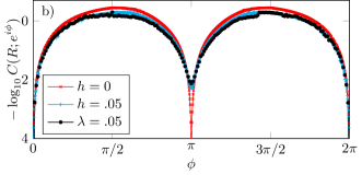
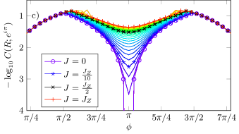
b) Cost for ribbons found using alternating minimization on the QDI2 model with . In the case a pair of , bond dimension 1 ribbons were sought, in the other cases, the pair consisted of a and a ribbon with bond dimensions and respectively. At the exactly solvable points (), we see a dramatic cost decrease at th roots of unity, signalling both the presence of and type of topological order present in these models. This feature remains even with the addition of an field or Ising type term which destroys the solvability of the model.
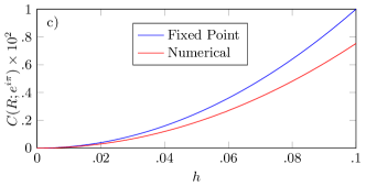
c) Cost of a width 4 ribbon of bond dimension 2 in the QDI2 model. The cost obtained from our numerical optimization is smaller than that of the fixed point string for all (nonzero) values of . This demonstrates the nontrivial nature of the ribbon operators we obtain, even in this perturbative regime.
When , this is a topologically ordered commuting model which reduces to the toric code when . This model also captures a number of other models, including the paramagnet () and a ferromagnet (). These latter correspond to distinct topologically trivial phases. At the fixed point of each of these phases, the model is exactly solvable. In the case, the generic model with is given by the Hamiltonian
| (26) |
At the RG fixed points of these phases (corresponding to either or ), we can set and , where / correspond to the / eigenstates of the relevant operator (i.e. the eigenstates of when and of when ). These ribbons commute with the Hamiltonian. Since , their -commutation relation is not unique, so they do not correspond to good ribbon operators. We therefore expect to be able to find zero-cost ribbons for all at these points. We note that constraining the ribbons to be unitary would be a natural way to eliminate these spurious solutions in the trivial phases, but this is computationally expensive; we discuss this point further in Sec. VII.
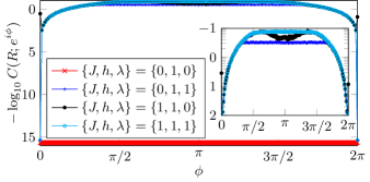
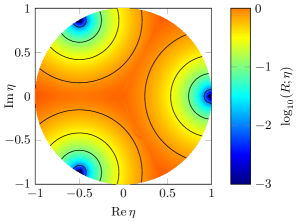
Costs for ribbons at various non-topological points in the QDId model are shown in Fig. 2. We observe two distinct ways in which trivial order can be signalled. As we have already discussed, one of these corresponds to mutually annihilating operators as in the para- and ferromagnetic phases. In the other case we simply fail to observe any low cost ribbons which form a nontrivial algebra. There are two explanations for this. Either there are no ribbon operators to be found or the chosen width is too narrow.
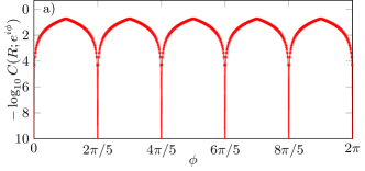
The phase which includes the point is topologically ordered, and we expect it to show a signal of -topological order. We therefore expect to observe low cost ribbons only when is a th root of 1. This property is expected to persist away from the exactly solvable point. In Fig. 3 we show the data obtained at the fixed points of the and models and when an field is turned on in the latter. As expected, at the fixed point a very strong signal is observed. Using a large density of points we see that the cost drops dramatically over a very narrow region around the th root of unity. When we turn on the field term, the signal decreases in magnitude but is still unmistakable, with more than two orders of magnitude in total contrast. Despite the clear signal, we observe that the value of the cost function at the minimum is comparable to the (square of) the perturbation strength. This may lead one to suspect that the method is simply returning the analytically obtainable fixed point ribbon. To refute this hypothesis, in Fig. 3c, we compare the cost of numerically obtained ribbons to those of the fixed point strings. Encouragingly, we see that the cost is smaller for the optimized ribbon, indicating that the method is finding a nontrivial result.
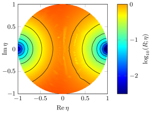
In Fig. 4, we present cost data for the fixed point of the QDI3 model over the entire unit disk. As expected, low cost ribbons can only be found around the third root of unity, with no minima occurring inside the disk. This property persists even when an field is turned on as shown in Fig. 5. This figure shows the cost of ribbons in the QDI2 model with . Even at this nonintegrable point, no low cost ribbons can be found anywhere away from the th roots of unity.
V.2 The Quantum Compass Model
It is interesting to consider the 2D quantum compass (QC) or Bacon-Shor modelDorier et al. (2005); Bacon (2006) in the context of ribbon operators. This model is defined on a square lattice with Hamiltonian
| (27) |
This model fails to exhibit many of the features expected of a topologically ordered model. For example, the ground state degeneracy does not depend on the underlying lattice topology. Moreover, this appears to be a gapless model with exponential ground state degeneracy.Dorier et al. (2005) Thus, this Hamiltonian is usually described as not having topological order. However, this model can be used to encode a qubit which is protected against arbitrary local errors, having a code distance extensive in the (linear) lattice size,Bacon (2006) a property which is clearly required of a topological code. This qubit can be defined by the pair of logical operators and . These operators commute with each Hamiltonian term, and intersect at a single point, hence they anticommute, , and therefore almost fulfill the conditions we give to be good ribbon operators. We will see below that they are rigid objects that exist due to special lattice symmetries, and they are not deformable.
The Hamiltonian Eq. (27) also commutes with all elements of the stabilizer group
| (28) |
It is therefore clear that () is related to () by application of a stabilizer element, and so defines the same encoded qubit in the ground space. Hence, the logical operators can be moved along to parallel strips.
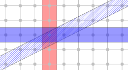
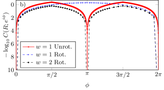
To investigate topological order in the QC model, we seek to find logical operators supported on rotated regions as shown in Fig. 6 or widened versions thereof. We compare this to the quantum double model where topological order is well understood.
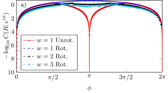
a) Cost of ribbons in the quantum compass model of Eq. (27). Because ribbons in this model are sensitive to their support, we conclude that they do not represent genuine topological order.
b) Cost of ribbons in the QDI2 model of Eq. (24) using . Note that the unit cell in the rotated case is rather than for convenience. Low cost ribbons can be found on both unrotated and rotated supports indicating genuine topological order.
In Fig. 7 we show the cost for ribbons obtained in these two models where the vertical ribbons are fixed to be and a bond dimension ribbon is optimized with both horizontal and rotated support. As discussed above, zero cost ribbons can be obtained for both models in the unrotated case when . Thus we see that each model supports a topologically encoded qubit. Once we rotate the ribbons, we find that in both cases the ribbon disappears when we restrict to . In the QDI2, the ribbon is recovered once we allow the support to grow to , however in the QC model there is no indication of a good ribbon existing even when we allow ribbons of width . This indicates that the low cost ribbons in the QC model are anomalies associated to lattice symmetries instead of genuine signatures of topological order.
V.3 Kitaev’s Honeycomb Model
The honeycomb modelKitaev (2006) is a frustrated spin model on the honeycomb lattice with Hamiltonian
| (29) |
where the , , and links refer to the three orientations of edges on the lattice. For , this model supports a phase with the same order as the quantum double model.Kitaev (2006) Writing a pair of anticommuting logical operators for this phase is a nontrivial task however, since they cannot both be symmetries of the Hamiltonian and will hence not have completely localized support. We can instead attempt to describe them with ribbons having some width .
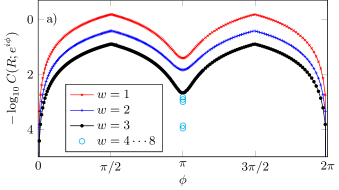
a) Cost for a bond dimension 5 ribbon on the honeycomb model of Eq. (29) with using . A second ribbon can be obtained analytically, and was fixed as a product of s along the and links of the lattice. The dip at is characteristic of order, and indicates the topological nature of this phase.
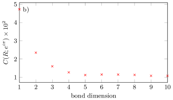
b) Cost for a width 2 ribbon at on the Honeycomb model with as a function of bond dimension. The cost rapidly saturates to a minimum, justifying our assumption that only small bond dimension is required.
c) As we increase the strength of , we eventually cross a phase transition to a gapless phase at (indicated by ). Approaching this point, the signal of topological order essentially vanishes. Here the strength of is increased in steps of from () to (). Note that the line marked by corresponds to plots and a bond dimension of is used for a width ribbon.
In Fig. 8, we investigate ribbon operators for the honeycomb model. As before, we observe the characteristic dip at signalling a topologically ordered phase (Fig. 8a). We also observe the effect of increasing the allowed ribbon width in Fig. 8a. As expected the cost goes down as the width increases, although this is not a smooth decrease. We suggest that this is due to the nature of the widening. Each time the width is increased by three, an additional plaquette lies completely within the support of . These plaquettes commute with the Hamiltonian, and so correspond to conserved quantities. In the perturbative regime, these plaquettes become those in the toric code model, which are associated with the location of anyonic charge. We note that the correlation length for is approximately ,Yang et al. (2008) so all of the widths correspond to several correlation lengths.
We also investigate how restricting the bond dimensions affects the cost. In Fig. 8b, we use a fixed width (3) and a fixed strength of . At this point, we see that the cost rapidly saturates to a minimum for a small bond dimension of 4-5. This justifies the relatively small bond dimensions used in this work.
Finally, we examine the effect of increasing the strength of in Fig. 8c. When , the model undergoes a transition from a phase supporting topological order to a gapless phase. The latter supports Ising anyons if a time reversal symmetry breaking term is added.Kitaev (2006) Although we do not see a strong signal, such as a discontinuity, at this point, we see that the dip associated with becomes very shallow. We expect the width of the required ribbons to be comparable to the correlation length, which we expect to increase as we move out of the perturbative regime. Thus the width ribbon used here is expected to be inadequate for large even within the phase. It remains to be seen whether ribbon operators can be used to identify phase transitions, possibly using a scaling analysis of ribbon width and bond dimension.
VI Ribbons As Logical Operators
One of the motivations for the ribbon operator methods is an application to quantum error correcting codes. In this section we show how nontrivial ribbon operators with sufficiently low cost can be used to certify the existence of an approximate topological quantum error correcting code in the ground space of the model. The ribbon operators function as approximate logical operators for these approximate codes. For gapped phases, this will also provide a natural justification for the method, although to apply this justification to the numerical results of Sec. V would require similar proofs with weaker assumptions than we are currently able to make here.
Let be a Hamiltonian with gap and suppose that for some , and , there exist ribbon operators and such that , , and . Here , we restrict to hermitian ribbons, and we let denote the operator norm. Let be some ground state of with energy . Then the expected energy of is
| (30) |
Thus, is a low energy state, and we can interpret as a generator for a unitary approximate logical operator.
It is important to check that is not mapping out of the ground space, so we need to ensure that there is a large overlap. Let denote the ground space projector for . By assumption the model has a spectral gap , so we find that
| (31) |
Rearranging this, and noting that can always be set to , we obtain
| (32) |
Thus, the action of the ribbon operators approximately preserves the ground space as long as they approximately preserve the norm of the individual ground states (). If this condition does not hold, is annihilating the ground space.
Given an almost commuting pair of hermitian operators and , we can perturb to an exactly commuting hermitian pair and such that the following holds:Lin (1997); Hastings (2009) and , where can be taken to be at most . It is convenient to work with and since they can be simultaneously exactly diagonalized. We need to check that the assumed twisted commutation relation between and is approximately maintained when we consider and .
| (33) |
Rearranging and using standard inequalities, we find
| (34) |
and so the twisted commutator is approximately preserved. The same argument shows that approximately commutes with and thus approximately preserves its ground space.
We now check that the action of on eigenstates of maps to a nearly orthogonal state and can therefore be used to manipulate information in the code space. Since and exactly commute, we can find a joint eigenstate such that and , then
| (35) |
and therefore
| (36) |
We have already assumed that maps a ground state to an approximately normalized state, so . Therefore, the action of maps to an approximately orthogonal state.
Thus, even approximate ribbon operators preserve the ground space (or annihilate it). Together, these results provide a certificate of topological order, at least when the strong assumptions of the derivation are met. In addition to providing such a certificate, this also shows that the method of ribbon operators can be used to obtain approximate logical operators even if the topological phase is already known. The ribbons can be used to enact logical operations on encoded qudits even when the underlying model is not an exact topological quantum code, such as in the case of the honeycomb model.
Recent work has investigated the possibility of certifying degeneracy in the ground space of a Hamiltonian using “approximate symmetries”.Chubb and Flammia (2016) In the case of unitary ribbons and , the authors showed that if , , and are sufficiently small, then the degeneracy of the ground space can indeed be certified as larger than some integer specified by . In the nontrivial case (i.e. ground space degeneracy larger than 1), the operators act as approximate logical operators when restricted to the ground space. One could utilize this result, along with the numerical procedures outlined in this work, to prove topological degeneracy by investigating the behavior of the cost function on different manifolds.
VII Summary and Outlook
We have introduced the method of ribbon operators for detecting topological order. By identifying features expected in topologically ordered spin models, we have defined a cost function which quantifies the extent to which operators on the lattice realize these features.
Using a variational minimization algorithm on this cost function over the space of matrix product operators, we have demonstrated that this method can distinguish nontrivial topological order from non-topological phases in various models, both integrable and nonintegrable. We have also shown how, with additional assumptions, ribbon operators can be used as approximate logical operators in topological quantum error correcting codes, which provides a specific sense in which they can certify the presence of topological order.
The most obvious open question is to extend these methods to other models, including those with nonabelian topological order. These nonabelian models are particularly interesting from a quantum information perspective as they can be utilized for universal quantum computation.Kitaev (2003); Nayak et al. (2008) Another open question is whether this method can be extended to detect symmetry-protected or symmetry-enriched topological order, but this would seem to require new ideas.
Even without generalizing the method to deal with nonabelian models, there are several natural ways in which our approach can be improved and extended. One could proceed by either changing the cost function, the variational class, or the optimization method. We begin by discussing a natural restriction on the allowed MPOs.
As shown in Sec. V.1, some topologically trivial models support zero-cost ribbon operators when the variational class is all MPOs of a given bond dimension. These operators corresponded to products of projectors onto local ground states. Although such operators have low cost, they are not good signals of topological order, since the for which is not unique because and mutually annihilate. This behavior could be removed by insisting that the ribbon operators be unitary. In addition to removing these false signals, a unitary constraint would ensure that ribbon operators properly preserve the norm of states on which they act. As discussed in Sec. VI, this property is important if the ribbons are to be interpreted as approximate logical operators for a quantum error correcting code.
A potential failure mode for this method is ‘high-temperature topological order’. Suppose there is some gapped state high up in the spectrum of the Hamiltonian, for example, at the top of the spectrum. It is conceivable that such a state could posess a ‘topological order’ distinct from the low-energy space. In this case, the method may find signals of TO which are originating from the high-energy portion of the spectrum. Such a failure mode could be combated by incorporating a low-temperature thermal state into the cost function. This would bias the norm towards the low-energy space, without the need for computing the ground state itself. Note that low temperature thermal states have efficient PEPS descriptions,Hastings (2006); Molnár et al. (2005) so the computational benefits of this method may remain.
One may also consider applying the method to seek out such high-energy topologically ordered subspaces in models with trivial ground spaces. This may provide an avenue towards interesting thermal physics with a topological flavor.
There are various alterations which can be made to the cost function defined in Sec. II.2. Recall that our cost function used the -commutator to incorporate the topological data. This is associated with the matrix of the anyon model. A natural replacement for, or addition to, this term would be a term involving the matrix. It is an open question if the current method or any of these suggested generalizations can be used to obtain the complete and matrices of a model. Recall from Sec. II that in the abelian case, there is a column permutation of which cannot be fixed. This could be addressed by ensuring all ribbons lie on comparable supports, for example circles or L shaped regions.
As discussed in Sec. II, insisting that a ribbon commute with the Hamiltonian on all eigenspaces (e.g. using the Frobenius norm ) is probably too strong to identify the topological order present in all models. One usually discusses topological order only with respect to the low-energy sector of the model. We propose that rather than taking the norm of the commutator, a variational low-energy state, for example in PEPSSchuch et al. (2010) or MERAVidal (2008) form, could be used to supplement the algorithm. Alternatively, one could use a low-energy thermal state as discussed above. Rather than evaluating norms, one could evaluate expectation values on these low energy states. This bypasses problems associated with finding ground states of 2D Hamiltonians, since the state need only be low energy and supported on a strip only just wider than the ribbon itself. Access to a state may be required for the extension to nonabelian models, where the excited spectrum is expected to be more exotic than in the abelian case and reflect the structure of the fusion space of the underlying anyons.
It would be interesting to apply the method to models where the topological order is still debated, for example the Heisenberg model on the Kagome lattice. When our cost function is encoded into an MPO for minimization using DMRG, it has a large bond dimensions since it is quadratic in the Hamiltonian of the model. This makes it computationally expensive to minimize. To approach these more complex models, it may be necessary to make use of properties of this MPO, such as sparsity, to reduce this cost. Alternatively, one could modify the cost function to reduce the bond dimension, or use another method to minimize it.
The assumptions used in Sec. VI are stronger than the constraints imposed in our numerical work. Understanding how to weaken these assumptions would provide additional justification for this method, and may provide insight into possible additional constraints which a ribbon operator should obey to ensure it is truly certifying topological order. It would also be interesting to blend our algorithm with the results of Chubb and Flammia (2016) with a view to certifying topological degeneracy.
Acknowledgements.
We thank Matthias Bal, Parsa Bonderson, Christopher Chubb, Andrew Doherty, Christopher Granade, Jeongwan Haah, Jutho Haegeman, Robert Pfeifer, Sam Roberts, Norbert Schuch, Tom Stace, Frank Verstraete and Dominic Williamson for useful and enlightening discussions. We also thank the anonymous referee who pointed out the potential failure mode that may result from a model with high-energy topologically ordered subspaces. We acknowledge support from the Australian Research Council via the Centre of Excellence in Engineered Quantum Systems (EQuS), project number CE110001013. STF also acknowledges support from an Australian Research Council Future Fellowship FT130101744. This work was initiated while DP was on sabbatical leave at The University of Sydney, he acknowledges their hospitality and their International Research Collaboration Award for partial support.References
- Wen (2013) Xiao-Gang Wen, “Topological Order: From Long-Range Entangled Quantum Matter to a Unified Origin of Light and Electrons,” ISRN Condensed Matter Physics 2013, 198710 (2013), arXiv:1210.1281 .
- Chen et al. (2013) Xie Chen, Zheng-Cheng Gu, Zheng-Xin Liu, and Xiao-Gang Wen, “Symmetry protected topological orders and the group cohomology of their symmetry group,” Physical Review B 87, 155114 (2013), arXiv:1106.4772 .
- Barkeshli et al. (2014) Maissam Barkeshli, Parsa Bonderson, Meng Cheng, and Zhenghan Wang, “Symmetry, Defects, and Gauging of Topological Phases,” arXiv:1410.4540 (2014).
- Anderson (1987) Phillip W. Anderson, “The Resonating Valence Bond State in La2CuO4 and Superconductivity,” Science 235, 1196–1198 (1987).
- Kitaev (2003) A. Yu Kitaev, “Fault-tolerant quantum computation by anyons,” Annals of Physics 303, 2–30 (2003), arXiv:quant-ph/9707021 .
- Nayak et al. (2008) Chetan Nayak, Steven H. Simon, Ady Stern, Michael Freedman, and Sankar Das Sarma, “Non-abelian anyons and topological quantum computation,” Reviews of Modern Physics 80, 1083 (2008), arXiv:0707.1889 .
- Wen and Niu (1990) X. G. Wen and Q. Niu, “Ground-state degeneracy of the fractional quantum Hall states in the presence of a random potential and on high-genus Riemann surfaces,” Physical Review B 41, 9377–9396 (1990).
- Dennis et al. (2002) Eric Dennis, Alexei Kitaev, Andrew Landahl, and John Preskill, “Topological quantum memory,” Journal of Mathematical Physics 43, 4452 (2002), arXiv:0110143 .
- Brown et al. (2014) Benjamin J. Brown, Daniel Loss, Jiannis K. Pachos, Chris N. Self, and James R Wootton, “Quantum memories at finite temperature,” arXiv:1411.6643 (2014).
- Terhal (2015) Barbara M. Terhal, “Quantum error correction for quantum memories,” Reviews of Modern Physics 87, 307 (2015), arXiv:1302.3428 .
- Brell et al. (2014) Courtney G. Brell, Simon Burton, Guillaume Dauphinais, Steven T. Flammia, and David Poulin, “Thermalization, Error Correction, and Memory Lifetime for Ising Anyon Systems,” Physical Review X 4, 031058 (2014), arXiv:1311.0019 .
- Levin and Wen (2006) Michael Levin and Xiao-Gang Wen, “Detecting Topological Order in a Ground State Wave Function,” Physical Review Letters 96, 110405 (2006), arXiv:cond-mat/0510613 .
- Kitaev and Preskill (2006) Alexei Kitaev and John Preskill, “Topological Entanglement Entropy,” Physical Review Letters 96, 110404 (2006), arXiv:hep-th/0510092 [hep-th] .
- Flammia et al. (2009) Steven T. Flammia, Alioscia Hamma, Taylor L. Hughes, and Xiao-Gang Wen, “Topological entanglement Rényi entropy and reduced density matrix structure,” Physical Review Letters 103, 261601 (2009), arXiv:0909.3305 .
- Isakov et al. (2011) Sergei V. Isakov, Matthew B. Hastings, and Roger G. Melko, “Topological entanglement entropy of a Bose-Hubbard spin liquid,” Nature Physics 7, 772–775 (2011), arXiv:1102.1721 .
- Zhang et al. (2012) Yi Zhang, Tarun Grover, Ari Turner, Masaki Oshikawa, and Ashvin Vishwanath, “Quasiparticle statistics and braiding from ground-state entanglement,” Physical Review B 85, 235151 (2012), arXiv:1111.2342 .
- Jiang et al. (2012) Hong-Chen Jiang, Zhenghan Wang, and Leon Balents, “Identifying topological order by entanglement entropy,” Nature Physics 8, 902–905 (2012), arXiv:1205.4289 .
- Li and Haldane (2008) Hui Li and F. D. M. Haldane, “Entanglement Spectrum as a Generalization of Entanglement Entropy: Identification of Topological Order in Non-Abelian Fractional Quantum Hall Effect States,” Physical Review Letters 101, 010504 (2008), arXiv:0805.0332 .
- Trebst et al. (2007) Simon Trebst, Philipp Werner, Matthias Troyer, Kirill Shtengel, and Chetan Nayak, “Breakdown of a Topological Phase: Quantum Phase Transition in a Loop Gas Model with Tension,” Physical Review Letters 98, 070602 (2007), arXiv:cond-mat/0609048 .
- Cincio and Vidal (2013) L. Cincio and G. Vidal, “Characterizing topological order by studying the ground states on an infinite cylinder,” Physical Review Letters 110, 067208 (2013), arXiv:1208.2623 .
- Buerschaper (2014) Oliver Buerschaper, “Twisted Injectivity in PEPS and the Classification of Quantum Phases,” Annals of Physics 351, 447–476 (2014), arXiv:1307.7763 .
- Schuch et al. (2010) Norbert Schuch, Ignacio Cirac, and David Pérez-García, “PEPS as ground states: Degeneracy and topology,” Annals of Physics 325, 2153–2192 (2010), arXiv:1001.3807 .
- Şahinoğlu et al. (2014) Mehmet Burak Şahinoğlu, Dominic Williamson, Nick Bultinck, Michael Mariën, Jutho Haegeman, Norbert Schuch, and Frank Verstraete, “Characterizing Topological Order with Matrix Product Operators,” arXiv:1409.2150 (2014).
- Bultinck et al. (2015) Nick Bultinck, Michael Mariën, Dominic Williamson, Mehmet Burak Şahinoğlu, Jutho Haegeman, and Frank Verstraete, “Anyons and matrix product operator algebras,” arXiv:1511.08090 (2015).
- Liu and Wen (2015) Fangzhou Liu and Xiao-Gang Wen, “Environment tensor as order parameter for symmetry breaking and (symmetry-protected) topological orders,” arXiv:1504.08365 (2015) .
- Evenbly and Vidal (2010) G. Evenbly and G. Vidal, “Frustrated antiferromagnets with entanglement renormalization: Ground state of the spin-1/2 heisenberg model on a kagome lattice,” Physical Review Letters 104, 187203 (2010), arXiv:0904.3383 .
- Yan et al. (2011) S. Yan, D. A. Huse, and S. R. White, “Spin-Liquid Ground State of the S = 1/2 Kagome Heisenberg Antiferromagnet,” Science 332, 1173–1176 (2011), arXiv:1011.6114 .
- Schollwöck (2011) Ulrich Schollwöck, “The density-matrix renormalization group in the age of matrix product states,” Annals of Physics 326, 96–192 (2011), arXiv:1008.3477 .
- (29) Liujun Zou, Jeongwan Haah, and Todari Senthil, In preparation .
- Chandran et al. (2014) Anushya Chandran, Vedika Khemani, and S. L. Sondhi, “How Universal Is the Entanglement Spectrum?” Physical Review Letters 113, 060501 (2014), arXiv:1311.2946 .
- Levin and Wen (2005) Michael Levin and Xiao-Gang Wen, “String-net condensation: A physical mechanism for topological phases,” Physical Review B 71, 045110 (2005), arXiv:cond-mat/0404617 .
- Nussinov and Ortiz (2009) Zohar Nussinov and Gerardo Ortiz, “Symmetry and Topological Order,” Proceedings of the National Academy of Sciences 106, 16944 (2009), arXiv:cond-mat/0605316 .
- (33) Zohar Nussinov and Gerardo Ortiz, “A symmetry principle for Topological Quantum Order,” Annals of Physics 324, 977 (2009), arXiv:cond-mat/0702377 .
- Cirac et al. (2011) J. Ignacio Cirac, Didier Poilblanc, Norbert Schuch, and Frank Verstraete, “Entanglement spectrum and boundary theories with projected entangled-pair states,” Physical Review B 83, 245134 (2011), arXiv:1103.3427 .
- Freedman et al. (2008) Michael Freedman, Chetan Nayak, and Kirill Shtengel, “Lieb-Schultz-Mattis theorem for quasi-topological systems,” Physical Review B 78, 174411 (2008), arXiv:cond-mat/0608508 .
- Haah (2011) Jeongwan Haah, “Local stabilizer codes in three dimensions without string logical operators,” Physical Review A 83, 042330 (2011), arXiv:1101.1962 .
- Kitaev (2006) Alexei Kitaev, “Anyons in an exactly solved model and beyond,” Annals of Physics 321, 2–111 (2006), arXiv:cond-mat/0506438 .
- Yang et al. (2008) Shuo Yang, Shi-Jian Gu, Chang-Pu Sun, and Hai-Qing Lin, “Fidelity susceptibility and long-range correlation in the Kitaev honeycomb model,” Physical Review A 78, 012304 (2008), arXiv:0803.1292 .
- Haah and Preskill (2012) Jeongwan Haah and John Preskill, “Logical-operator tradeoff for local quantum codes,” Physical Review A 86, 032308 (2012), arXiv:1011.3529 .
- Landon-Cardinal and Poulin (2013) Olivier Landon-Cardinal and David Poulin, “Local Topological Order Inhibits Thermal Stability in 2D,” Physical Review Letters 110, 090502 (2013), arXiv:1209.5750 .
- Hastings and Wen (2005) M. B. Hastings and Xiao-Gang Wen, “Quasiadiabatic continuation of quantum states: The stability of topological ground-state degeneracy and emergent gauge invariance,” Physical Review B 72, 045141 (2005), arXiv:cond-mat/0503554 .
- Haah (2016) Jeongwan Haah, “An invariant of topologically ordered states under local unitary transformations,” Communications in Mathematical Physics 342, 771–801 (2016), arXiv:1407.2926 .
- Pirvu et al. (2010) B. Pirvu, V. Murg, J. I. Cirac, and F. Verstraete, “Matrix product operator representations,” New Journal of Physics 12, 025012 (2010), arXiv:0804.3976 .
- Dorier et al. (2005) Julien Dorier, Federico Becca, and Frédéric Mila, “Quantum compass model on the square lattice,” Physical Review B 72, 024448 (2005), arXiv:cond-mat/0501708 .
- Bacon (2006) Dave Bacon, “Operator quantum error-correcting subsystems for self-correcting quantum memories,” Physical Review A 73, 012340 (2006), arXiv:quant-ph/0506023 .
- Lin (1997) Huaxin Lin, “Almost commuting selfadjoint matrices and applications,” in Operator algebras and their applications, Fields Institute Communications, Vol. 13 (American Mathematical Society, 1997) pp. 193–233.
- Hastings (2009) M. B. Hastings, “Making Almost Commuting Matrices Commute,” Communications in Mathematical Physics 291, 321–345 (2009), arXiv:0808.2474 .
- Chubb and Flammia (2016) Christopher T. Chubb and Steven T. Flammia, “Approximate symmetries of Hamiltonians,” arXiv:1608.02600 (2016) .
- Hastings (2006) M. B. Hastings, “Solving Gapped Hamiltonians Locally,” Physical Review B 73, 085115 (2006), arXiv:cond-mat/0508554 .
- Molnár et al. (2005) András Molnár, Norbert Schuch, Frank Verstraete, and Ignacio Cirac, “Approximating Gibbs states of local Hamiltonians efficiently with PEPS,” Physical Review B 91, 045138 (2015), arXiv:1406.2973 .
- Vidal (2008) G. Vidal, “Class of Quantum Many-Body States That Can Be Efficiently Simulated,” Physical Review Letters 101, 110501 (2008), arXiv:quant-ph/0610099 .
Appendix A Quantum Double
The cost function for a pair of width 1 ribbon operators in the quantum double model defined in Eq. 18 of the main document (with ) can easily be written. Define the lattice as in Fig. 1 of the main document, and let the strings and have supports on the horizontal and vertical strips respectively. Beginning with ribbon , we see that there are no Hamiltonian terms contained completely within the support. Thus the first term in the cost vanishes. The same happens for ribbon .
The next term concerns those Hamiltonian terms which cross the boundary. There are two classes, those with support on a single spin inside and those supported on a pair of spins in . Each dark plaquette (![]() ) contributes to a term in the first class, with each spin in being touched by a pair of such plaquettes. Therefore at this stage we have an initial cost function for the commutator part given by
) contributes to a term in the first class, with each spin in being touched by a pair of such plaquettes. Therefore at this stage we have an initial cost function for the commutator part given by
| (37) |
where is the number of spins on which is supported. Each light plaquette (![]() ) contributes a two-spin term, so the costs become
) contributes a two-spin term, so the costs become
| (38) |
For convenience, assume two-site translationally invariant product operators for both and . This cost function becomes
| (39) |
since of the sites of support operator and sites support operator .
There are no more terms contributed by the commutator with the Hamiltonian. It remains to include the twisted commutator terms. The ribbon can intersect with either a site or a site. Recall that we require that all translations of are considered, so we obtain
| (40) |
where is the operator at site of ribbon . Notice that each is required to commute with both and . In this way, the insensitivity of this term to the particular support of is ensured. This term gives
| (41) |
Combining these two costs, we obtain the total cost function for ribbon
| (42) | ||||
| (43) |
The cost for ribbon can be obtained analogously, giving
| (44) |
Notice that . Care should be taken with this term since is not symmetric in its arguments.
It is easy to check that, as expected, these cost functions are both zero when we set , and , corresponding to the known string operators for this model.