Robust imaging with electromagnetic waves in noisy environments

Liliana Borcea111Department of Mathematics, University of Michigan, Ann Arbor, MI 48109. borcea@umich.edu    Josselin Garnier222Laboratoire de Probabilités et Modèles Aléatoires & Laboratoire Jacques-Louis Lions, Université Paris Diderot, 75205 Paris Cedex 13, France. garnier@math.univ-paris-diderot.fr
Abstract

We study imaging with an array of sensors that probes a medium with single frequency electromagnetic waves and records the scattered electric field. The medium is known and homogenous except for some small and penetrable inclusions. The goal of inversion is to locate and characterize these inclusions from the data collected by the array, which are corrupted by additive noise. We use results from random matrix theory to obtain a robust inversion method. We assess its performance with numerical simulations and quantify the benefit of measuring more than one component of the scattered electric field.

keywords:
imaging, electromagnetic waves, random matrix theory.

1 Introduction

We study an inverse problem for Maxwell’s equations, where unknown scatterers in a medium are to be determined from data collected with an array of sources and receivers. The sources emit signals which propagate in the medium and the receivers record the backscattered waves. The recordings, indexed by the source and receiver pair, are the entries in the response matrix, the data, which are contaminated with additive noise.

Sensor array imaging is an important technology in nondestructive testing, medical imaging, radar, seismic exploration, and elsewhere. It operates over application specific ranges of frequencies and fixed or synthetic apertures. We consider imaging with single frequency waves and a fixed array of N𝑁N sensors that play the dual role of sources and receivers. The unknown scatterers lie in a homogeneous medium. They are P𝑃P penetrable inclusions of small size with respect to the wavelength. As shown in [5] they can be described by their center location ypsubscripty𝑝\vec{{{\itbf y}}}_{p} and reflectivity tensor 𝝆psubscript𝝆𝑝\bm{\rho}_{p} which depends on the volume and shape of their support, and their electric permittivity ϵpsubscriptitalic-ϵ𝑝\epsilon_{p}, for p=1,,P𝑝1𝑃p=1,\ldots,P.

There are many algorithms for locating scatterers from the response matrix. Reverse time or Kirchhoff migration [11] and the similar filtered backprojection [14] are common in seismic and radar imaging with broadband data. Matched field processing [7] is popular in underwater acoustics. Qualitative methods such as linear sampling [12], the factorization method [20], and the MUSIC (Multiple Signal Classification) algorithm [22] are useful for imaging with single frequency waves, and give high resolution results if the noise is weak.

A study of noise effects on the MUSIC method can be found in [16]. It determines upper bounds on the noise level that guarantee the exact recovery of point scatterers in a sparse scene. Here we consider stronger noise and use results from random matrix theory [10, 13, 8, 21] to obtain a robust MUSIC type localization method. Such results have led to scatterer detection tests in [3, 4], and to filters of backscattered waves in random media in [6, 1]. They are also the foundation of a robust sonar array imaging method of well separated point scatterers in [17]. We extend the results in [17] to electromagnetic waves, for locating one or more inclusions and estimating their reflectivity tensor. We also quantify the benefits of measuring more than one component of the scattered electric field.

The paper is organized as follows: We begin in section 2 with the mathematical formulation of the inverse problem, and then give in section 3 the data model. The singular value decomposition analysis of the response matrix is described in section 4. The inversion method uses this analysis and is presented in section 5. Numerical simulation results are shown in section 6. We end with a summary in section 7.

2 Formulation of the problem

Consider a homogeneous isotropic medium with electric permittivity ϵosubscriptitalic-ϵ𝑜\epsilon_{o} and magnetic permeability μosubscript𝜇𝑜\mu_{o}, which contains P𝑃P penetrable inclusions supported in the disjoint simply connected domains ΩpsubscriptΩ𝑝\Omega_{p} with smooth boundaries, centered at locations ypsubscripty𝑝\vec{{{\itbf y}}}_{p}, for p=1,,P𝑝1𝑃p=1,\ldots,P. The inclusions are modelled by the piecewise constant electric permittivity

ϵ(x)=p=1Pϵp1Ωp(x)+ϵo13Ω(x),Ω=p=1PΩp,formulae-sequenceitalic-ϵxsuperscriptsubscript𝑝1𝑃subscriptitalic-ϵ𝑝subscript1subscriptΩ𝑝xsubscriptitalic-ϵ𝑜subscript1superscript3ΩxΩsuperscriptsubscript𝑝1𝑃subscriptΩ𝑝\epsilon(\vec{{{\itbf x}}})=\sum_{p=1}^{P}\epsilon_{p}1_{\Omega_{p}}(\vec{{{\itbf x}}})+\epsilon_{o}1_{\mathbb{R}^{3}\setminus\Omega}(\vec{{{\itbf x}}}),\qquad\Omega=\bigcup_{p=1}^{P}\Omega_{p}, (1)

where 1Ω(x)subscript1Ωx1_{\Omega}(\vec{{{\itbf x}}}) is the indicator function of the domain ΩΩ\Omega, and ϵpsubscriptitalic-ϵ𝑝\epsilon_{p} are scalar real valued for p=1,,P𝑝1𝑃p=1,\ldots,P.

The medium is probed with N𝑁N sensors that are both sources and receivers. They are closely spaced at locations {xr}1rNsubscriptsubscriptx𝑟1𝑟𝑁\{\vec{{{\itbf x}}}_{r}\}_{1\leq r\leq N} in a set 𝒜𝒜\mathcal{A}, so they behave like a collective entity, the array. For convenience we let 𝒜𝒜\mathcal{A} be planar and square, of side a𝑎a, the array aperture. This allows us to introduce a system of coordinates with origin at the center of the array and orthonormal basis {e1,e2,e3}subscripte1subscripte2subscripte3\{\vec{{{\itbf e}}}_{1},\vec{{{\itbf e}}}_{2},\vec{{{\itbf e}}}_{3}\}. The vectors e1,e2subscripte1subscripte2\vec{{{\itbf e}}}_{1},\vec{{{\itbf e}}}_{2} span the plane of the array, named the cross-range plane, and the line along e3subscripte3\vec{{{\itbf e}}}_{3} is the range direction. The distance between the array and the inclusions is of order L𝐿L, the range scale. See Figure 1 for an illustration.

Refer to caption𝒜𝒜\mathcal{A}a𝑎aL𝐿Le2subscripte2\vec{{{\itbf e}}}_{2}e1subscripte1\vec{{{\itbf e}}}_{1}e3subscripte3\vec{{{\itbf e}}}_{3}y1subscripty1\vec{{{\itbf y}}}_{1}y2subscripty2\vec{{{\itbf y}}}_{2}y3subscripty3\vec{{{\itbf y}}}_{3}
Fig. 1: Illustration of the inversion setup. The array 𝒜𝒜\mathcal{A} is square planar with side a𝑎a, in the cross-range plane spanned by e1subscripte1\vec{{{\itbf e}}}_{1} and e2subscripte2\vec{{{\itbf e}}}_{2}. The imaging region is at range scale L𝐿L from the array. In the illustration there are three inclusions at locations ypsubscripty𝑝\vec{{{\itbf y}}}_{p}, for p=1,2,3.𝑝123p=1,2,3.

We index consistently a source sensor by s𝑠s and a receiver sensor by r𝑟r, altough both s𝑠s and r𝑟r take values in the same set {1,,N}1𝑁\{1,\ldots,N\}. The sources are point dipoles with current density jsδ(xxs)subscriptj𝑠𝛿xsubscriptx𝑠\vec{\itbf j}_{s}\delta(\vec{{{\itbf x}}}-\vec{{{\itbf x}}}_{s}), and the resulting electric field EE\vec{{\itbf E}} satisfies

××E(x;xs)k2ϵ(x)ϵoE(x;xs)=ikμoϵojsδ(xxs),Exsubscriptx𝑠superscript𝑘2italic-ϵxsubscriptitalic-ϵ𝑜Exsubscriptx𝑠𝑖𝑘subscript𝜇𝑜subscriptitalic-ϵ𝑜subscriptj𝑠𝛿xsubscriptx𝑠\displaystyle\vec{\nabla}\times\vec{\nabla}\times\vec{{\itbf E}}(\vec{{{\itbf x}}};\vec{{{\itbf x}}}_{s})-k^{2}\frac{\epsilon(\vec{{{\itbf x}}})}{\epsilon_{o}}\vec{{\itbf E}}(\vec{{{\itbf x}}};\vec{{{\itbf x}}}_{s})=ik\sqrt{\frac{\mu_{o}}{\epsilon_{o}}}\,\vec{\itbf j}_{s}\delta(\vec{{{\itbf x}}}-\vec{{{\itbf x}}}_{s}), (2)

and the radiation condition

lim|x||x|[×E(x;xs)ikx|x|×E(x;xs)]=0.subscriptxxdelimited-[]Exsubscriptx𝑠𝑖𝑘xxExsubscriptx𝑠0\lim_{|\vec{{{\itbf x}}}|\to\infty}|\vec{{{\itbf x}}}|\left[\vec{\nabla}\times\vec{{\itbf E}}(\vec{{{\itbf x}}};\vec{{{\itbf x}}}_{s})-ik\frac{\vec{{{\itbf x}}}}{|\vec{{{\itbf x}}}|}\times\vec{{\itbf E}}(\vec{{{\itbf x}}};\vec{{{\itbf x}}}_{s})\right]=0. (3)

Equation (3) is derived from Maxwell’s equations at frequency ω𝜔\omega, and

k=ωco=2πλ𝑘𝜔subscript𝑐𝑜2𝜋𝜆k=\frac{\omega}{c_{o}}=\frac{2\pi}{\lambda}

is the wavenumber, where co=1/μoϵosubscript𝑐𝑜1subscript𝜇𝑜subscriptitalic-ϵ𝑜c_{o}=1/\sqrt{\mu_{o}\epsilon_{o}} is the wave speed and λ𝜆\lambda is the wavelength.

We decompose EE\vec{{\itbf E}} in the direct field EosubscriptE𝑜\vec{{\itbf E}}_{o} and the scattered one denoted by 𝓔𝓔\vec{\bm{\mathcal{E}}},

𝓔(x;xs)=E(x;xs)Eo(x;xs).𝓔xsubscriptx𝑠Exsubscriptx𝑠subscriptE𝑜xsubscriptx𝑠\vec{\bm{\mathcal{E}}}(\vec{{{\itbf x}}};\vec{{{\itbf x}}}_{s})=\vec{{\itbf E}}(\vec{{{\itbf x}}};\vec{{{\itbf x}}}_{s})-\vec{{\itbf E}}_{o}(\vec{{{\itbf x}}};\vec{{{\itbf x}}}_{s}). (4)

The direct field solves the analogue of (2)–(3) in the homogeneous medium, and can be written explicitly as

Eo(x;xs)=ikμoϵo𝐆(x,xs)js,subscriptE𝑜xsubscriptx𝑠𝑖𝑘subscript𝜇𝑜subscriptitalic-ϵ𝑜𝐆xsubscriptx𝑠subscriptj𝑠\vec{{\itbf E}}_{o}(\vec{{{\itbf x}}};\vec{{{\itbf x}}}_{s})=ik\sqrt{\frac{\mu_{o}}{\epsilon_{o}}}\,{\bf G}(\vec{{{\itbf x}}},\vec{{{\itbf x}}}_{s})\vec{\itbf j}_{s}, (5)

using the dyadic Green’s tensor

𝐆(x,z)=(𝐈3+Tk2)eik|xz|4π|xz|.𝐆xzsubscript𝐈3superscript𝑇superscript𝑘2superscript𝑒𝑖𝑘xz4𝜋xz{\bf G}(\vec{{{\itbf x}}},\vec{{{\itbf z}}})=\left({\bf I}_{3}+\frac{\nabla\nabla^{T}}{k^{2}}\right)\frac{e^{ik|\vec{{{\itbf x}}}-\vec{{{\itbf z}}}|}}{4\pi|\vec{{{\itbf x}}}-\vec{{{\itbf z}}}|}. (6)

The scattered field 𝓔𝓔\vec{\bm{\mathcal{E}}} is recorded at the N𝑁N receivers, and the experiment may be repeated by emitting waves sequentially from all the sources. Each source may use up to three illuminations, with linearly independent js3subscriptj𝑠superscript3\vec{\itbf j}_{s}\in\mathbb{R}^{3}, and the receivers may record one or all three components of 𝓔𝓔\vec{\bm{\mathcal{E}}}. We call the data for all possible illuminations and recordings complete. All other cases, with one or two illuminations from each source and one or two components of 𝓔𝓔\vec{\bm{\mathcal{E}}} measured at the receivers are called incomplete. The goal is to locate and characterize the inclusions using the complete or incomplete measurements.

We simplify the problem by assuming that the inclusions are small with respect to the wavelength, so we can represent them as in [5] by their center locations ypsubscripty𝑝\vec{{{\itbf y}}}_{p} and 3×3333\times 3 reflectivity tensors 𝝆psubscript𝝆𝑝\bm{\rho}_{p}, for p=1,,P𝑝1𝑃p=1,\ldots,P. These tensors depend on the shape of the domains ΩpsubscriptΩ𝑝\Omega_{p} and the relative electric permittivity ϵp/ϵosubscriptitalic-ϵ𝑝subscriptitalic-ϵ𝑜\epsilon_{p}/\epsilon_{o}. The inverse problem is to determine the locations ypsubscripty𝑝\vec{{{\itbf y}}}_{p} and reflectivity tensors 𝝆psubscript𝝆𝑝\bm{\rho}_{p} from the array measurements.

3 Data model

Let α𝛼\alpha be a small and positive dimensionless parameter which scales the size of the inclusions

[Vol(Ωp)]1/3λα1,p=1,,P,formulae-sequencesimilar-tosuperscriptdelimited-[]VolsubscriptΩ𝑝13𝜆𝛼much-less-than1𝑝1𝑃\frac{\left[{\rm Vol}(\Omega_{p})\right]^{1/3}}{\lambda}\sim\alpha\ll 1,\quad p=1,\ldots,P, (7)

and denote by 𝓔q(x;xs)subscript𝓔𝑞xsubscriptx𝑠\vec{\bm{\mathcal{E}}}_{q}(\vec{{{\itbf x}}};\vec{{{\itbf x}}}_{s}) the scattered field due to the source at xssubscriptx𝑠\vec{{{\itbf x}}}_{s}, with js=eqsubscriptj𝑠subscripte𝑞\vec{\itbf j}_{s}=\vec{{{\itbf e}}}_{q}. It has the following asymptotic expansion in the limit α0𝛼0\alpha\to 0, as shown in [5],

𝓔q(x;xs)=ik3μoϵop=1P𝐆(x,yp)𝝆p𝐆(yp,xs)eq+O(α4).subscript𝓔𝑞xsubscriptx𝑠𝑖superscript𝑘3subscript𝜇𝑜subscriptitalic-ϵ𝑜superscriptsubscript𝑝1𝑃𝐆xsubscripty𝑝subscript𝝆𝑝𝐆subscripty𝑝subscriptx𝑠subscripte𝑞𝑂superscript𝛼4\vec{\bm{\mathcal{E}}}_{q}(\vec{{{\itbf x}}};\vec{{{\itbf x}}}_{s})=ik^{3}\sqrt{\frac{\mu_{o}}{\epsilon_{o}}}\sum_{p=1}^{P}{\bf G}(\vec{{{\itbf x}}},\vec{{{\itbf y}}}_{p})\bm{\rho}_{p}{\bf G}(\vec{{{\itbf y}}}_{p},\vec{{{\itbf x}}}_{s})\vec{{{\itbf e}}}_{q}+O(\alpha^{4})\,. (8)

The reflectivity tensor of the mlimit-from𝑚m-th inclusion is defined by

𝝆p=α3(ϵpϵo1)𝐌p,subscript𝝆𝑝superscript𝛼3subscriptitalic-ϵ𝑝subscriptitalic-ϵ𝑜1subscript𝐌𝑝\bm{\rho}_{p}=\alpha^{3}\left(\frac{\epsilon_{p}}{\epsilon_{o}}-1\right){\bf M}_{p}, (9)

using the α𝛼\alpha-independent polarization tensor 𝐌psubscript𝐌𝑝{\bf M}_{p}. We refer to [5] for details on 𝐌psubscript𝐌𝑝{\bf M}_{p}, and to section 6 for its calculation in our numerical simulations. It suffices to say that 𝐌psubscript𝐌𝑝{\bf M}_{p} is a symmetric, real valued 3×3333\times 3 matrix which depends on the shape of ΩpsubscriptΩ𝑝\Omega_{p} and the relative electric permittivity ϵp/ϵosubscriptitalic-ϵ𝑝subscriptitalic-ϵ𝑜\epsilon_{p}/\epsilon_{o}.

3.1 The noiseless data model

Since k𝑘k, μosubscript𝜇𝑜\mu_{o} and ϵosubscriptitalic-ϵ𝑜\epsilon_{o} are known, let us model the noiseless data gathered with the receiver and source pair (r,s)𝑟𝑠(r,s) by

𝐝(xr,xs)=ϵo/μoik3(𝓔1,𝓔2,𝓔3),r,s=1,,N.formulae-sequence𝐝subscriptx𝑟subscriptx𝑠subscriptitalic-ϵ𝑜subscript𝜇𝑜𝑖superscript𝑘3subscript𝓔1subscript𝓔2subscript𝓔3𝑟𝑠1𝑁{{\bf d}}(\vec{{{\itbf x}}}_{r},\vec{{{\itbf x}}}_{s})=\frac{\sqrt{\epsilon_{o}/\mu_{o}}}{ik^{3}}\left(\vec{\bm{\mathcal{E}}}_{1},\vec{\bm{\mathcal{E}}}_{2},\vec{\bm{\mathcal{E}}}_{3}\right),\quad r,s=1,\ldots,N. (10)

This is a 3×3333\times 3 complex matrix, the (r,s)𝑟𝑠(r,s) block of the 3N×3N3𝑁3𝑁3N\times 3N complete data matrix 𝐃𝐃{{\bf D}} collected by the array,

𝐃=(𝐝(xr,xs))r,s=1,,N.𝐃subscript𝐝subscriptx𝑟subscriptx𝑠formulae-sequence𝑟𝑠1𝑁{{\bf D}}=\left({{\bf d}}(\vec{{{\itbf x}}}_{r},\vec{{{\itbf x}}}_{s})\right)_{r,s=1,\ldots,N}. (11)

To acquire 𝐃𝐃{{\bf D}} directly, the array would use the sources sequentially, with current densities eqδ(xxs)subscripte𝑞𝛿xsubscriptx𝑠\vec{{{\itbf e}}}_{q}\delta(\vec{{{\itbf x}}}-\vec{{{\itbf x}}}_{s}), for q=1,2,3𝑞123q=1,2,3 and s=1,,N𝑠1𝑁s=1,\ldots,N, and would measure the scattered fields 𝓔q(x;xs)subscript𝓔𝑞xsubscriptx𝑠\vec{\bm{\mathcal{E}}}_{q}(\vec{{{\itbf x}}};\vec{{{\itbf x}}}_{s}) at the receivers. This acquisition method is not optimal in noisy environments, and may be improved as explained in the next section.

When the sensors emit and receive only along one or two directions, we have incomplete measurements. Let us denote by 𝒮{1,2,3}𝒮123\mathscr{S}\subset\{1,2,3\} the set of indices of the measured components of the electric field, and define the 3×|𝒮|3𝒮3\times|\mathscr{S}| sensing matrix

𝐒=(eq)q𝒮,𝐒subscriptsubscripte𝑞𝑞𝒮{\bf S}=\left(\vec{{{\itbf e}}}_{q}\right)_{q\in\mathscr{S}}, (12)

with columns given by the unit vectors eqsubscripte𝑞\vec{{{\itbf e}}}_{q} with q𝒮𝑞𝒮q\in\mathscr{S}. We assume for convenience that the source excitation currents are also limited to these directions, and denote the incomplete data matrix by 𝐃Ssubscript𝐃𝑆{{\bf D}}_{{}_{S}}. It is a complex |𝒮|N×|𝒮|N𝒮𝑁𝒮𝑁|\mathscr{S}|N\times|\mathscr{S}|N matrix that can be written in terms of 𝐃𝐃{{\bf D}} as

𝐃S=diag(𝐒T,,𝐒T)𝐃diag(𝐒,,𝐒).subscript𝐃𝑆diagsuperscript𝐒𝑇superscript𝐒𝑇𝐃diag𝐒𝐒{{\bf D}}_{{}_{S}}=\mbox{diag}\left({\bf S}^{T},\ldots,{\bf S}^{T}\right){{\bf D}}\mbox{diag}\left({\bf S},\ldots,{\bf S}\right). (13)

The mathematical model of 𝐃𝐃{{\bf D}} follows from (8) and (10). We write it using the forward map 𝓕𝓕\bm{\mathscr{F}}, which takes the unknown locations and reflectivity tensors of the inclusions to the space 3N×3Nsuperscript3𝑁3𝑁\mathbb{C}^{3N\times 3N} of matrices where 𝐃𝐃{{\bf D}} lies,

𝐃𝐃\displaystyle{{\bf D}} 𝓕(y1,,yP,𝝆1,,𝝆P)=(p=1P𝐆(xr,yp)𝝆p𝐆(yp,xs))r,s=1,,N.absent𝓕subscripty1subscripty𝑃subscript𝝆1subscript𝝆𝑃subscriptsuperscriptsubscript𝑝1𝑃𝐆subscriptx𝑟subscripty𝑝subscript𝝆𝑝𝐆subscripty𝑝subscriptx𝑠formulae-sequence𝑟𝑠1𝑁\displaystyle\approx\bm{\mathscr{F}}(\vec{{{\itbf y}}}_{1},\ldots,\vec{{{\itbf y}}}_{P},\bm{\rho}_{1},\ldots,\bm{\rho}_{P})=\left(\sum_{p=1}^{P}{\bf G}(\vec{{{\itbf x}}}_{r},\vec{{{\itbf y}}}_{p})\bm{\rho}_{p}{\bf G}(\vec{{{\itbf y}}}_{p},\vec{{{\itbf x}}}_{s})\right)_{r,s=1,\ldots,N.} (14)

The forward map for the incomplete measurements is deduced from (13)–(14). We assume henceforth that 𝓕𝓕\bm{\mathscr{F}} gives a good approximation of 𝐃𝐃{{\bf D}}, as is the case for sufficiently small α𝛼\alpha, and treat the approximation in (14) as an equality.

3.2 Noisy data and the Hadamard acquisition scheme

In any practical setting the measurements are contaminated with noise, which may be mitigated by the data acquisition scheme, as we now explain.

Suppose that the N𝑁N sources do not emit waves sequentially, but at the same time, for 3N3𝑁3N experiments indexed by (n,q)𝑛𝑞(n,q), with n=1,,N𝑛1𝑁n=1,\ldots,N and q=1,2,3.𝑞123q=1,2,3. In the (n,q)𝑛𝑞(n,q) experiment the excitation from the source at xssubscriptx𝑠\vec{{{\itbf x}}}_{s} is js,(n,q)subscriptj𝑠𝑛𝑞\vec{\itbf j}_{s,(n,q)}, and gathering the measurements for q=1,2,3𝑞123q=1,2,3, we obtain the following model of the recordings at the receiver location xrsubscriptx𝑟\vec{{{\itbf x}}}_{r},

𝐝r,nH=s=1N𝐝(xr,xs)𝐣s,n+𝐰r,n.subscriptsuperscript𝐝H𝑟𝑛superscriptsubscript𝑠1𝑁𝐝subscriptx𝑟subscriptx𝑠subscript𝐣𝑠𝑛subscript𝐰𝑟𝑛{\bf d}^{\rm H}_{r,n}=\sum_{s=1}^{N}{{\bf d}}(\vec{{{\itbf x}}}_{r},\vec{{{\itbf x}}}_{s}){\bf j}_{s,n}+{\bf w}_{r,n}. (15)

This is a 3×3333\times 3 complex matrix, determined by 𝐝(xr,xs)𝐝subscriptx𝑟subscriptx𝑠{{\bf d}}(\vec{{{\itbf x}}}_{r},\vec{{{\itbf x}}}_{s}) defined in (10), the excitation matrices 𝐣s,nsubscript𝐣𝑠𝑛{\bf j}_{s,n} with columns js,(n,q)subscriptj𝑠𝑛𝑞\vec{\itbf j}_{s,(n,q)} for q=1,2,3𝑞123q=1,2,3, and the noise matrix 𝐰r,nsubscript𝐰𝑟𝑛{\bf w}_{r,n}. The complete 3N×3N3𝑁3𝑁3N\times 3N measurement matrix 𝐃Hsuperscript𝐃H{\bf D}^{\rm H} has the block structure

𝐃H=(𝐝r,nH)r,n=1,,N,superscript𝐃Hsubscriptsubscriptsuperscript𝐝H𝑟𝑛formulae-sequence𝑟𝑛1𝑁{\bf D}^{\rm H}=\left({\bf d}^{\rm H}_{r,n}\right)_{r,n=1,\ldots,N},

and it is modeled by

𝐃H=𝐃𝐉+𝓦,superscript𝐃H𝐃𝐉𝓦{\bf D}^{\rm H}={{\bf D}}{{{\bf J}}}+\bm{\mathcal{W}}, (16)

where 𝐉𝐉{{{\bf J}}} is the excitation matrix with blocks 𝐣s,nsubscript𝐣𝑠𝑛{\bf j}_{s,n} for s,n=1,,Nformulae-sequence𝑠𝑛1𝑁s,n=1,\ldots,N, and 𝓦𝓦\bm{\mathcal{W}} is the noise matrix with blocks 𝐰r,nsubscript𝐰𝑟𝑛{\bf w}_{r,n} for r,n=1,,Nformulae-sequence𝑟𝑛1𝑁r,n=1,\ldots,N.

We assume that the excitation currents are normalized so that the entries in 𝐉𝐉{{\bf J}} have unit amplitudes, and take as is usual a noise matrix 𝓦𝓦\bm{\mathcal{W}} with mean zero and independent complex Gaussian entries with standard deviation σ𝜎\sigma. This gives

𝔼[𝓦𝓦]=σ2𝐈3N,𝔼delimited-[]superscript𝓦𝓦superscript𝜎2subscript𝐈3𝑁\mathbb{E}\left[\bm{\mathcal{W}}^{\dagger}\bm{\mathcal{W}}\right]=\sigma^{2}{\bf I}_{{}_{3N}},

where \dagger denotes the complex conjugate and transpose, 𝔼𝔼\mathbb{E} is the expectation, and 𝐈3Nsubscript𝐈3𝑁{\bf I}_{{}_{3N}} is the 3N×3N3𝑁3𝑁3N\times 3N identity matrix. The acquisition scheme uses an invertible 𝐉𝐉\bm{{{\bf J}}}, to obtain

𝐃~=𝐃H𝐉1=𝐃+𝐖,𝐖=𝓦𝐉1.formulae-sequence~𝐃superscript𝐃Hsuperscript𝐉1𝐃𝐖𝐖𝓦superscript𝐉1\widetilde{{\bf D}}={\bf D}^{\rm H}{{\bf J}}^{-1}={{\bf D}}+{\bf W},\qquad{\bf W}=\bm{\mathcal{W}}{{\bf J}}^{-1}. (17)

This is a corrupted version of 𝐃𝐃{{\bf D}}, but the noise level in 𝐖𝐖{\bf W}, which has mean zero complex Gaussian entries, is reduced for a good choice of 𝐉𝐉{{{\bf J}}}. Such a choice would give

𝔼[𝐖𝐖]=(𝐉1)𝔼[𝓦𝓦]𝐉1=σ2(𝐉1)𝐉1=σ𝐖2𝐈3N,𝔼delimited-[]superscript𝐖𝐖superscriptsuperscript𝐉1𝔼delimited-[]superscript𝓦𝓦superscript𝐉1superscript𝜎2superscriptsuperscript𝐉1superscript𝐉1superscriptsubscript𝜎𝐖2subscript𝐈3𝑁\mathbb{E}\left[{\bf W}^{\dagger}{\bf W}\right]=\big{(}{{\bf J}}^{-1}\big{)}^{\dagger}\mathbb{E}\left[\bm{\mathcal{W}}^{\dagger}\bm{\mathcal{W}}\right]{{\bf J}}^{-1}=\sigma^{2}\big{(}{{\bf J}}^{-1}\big{)}^{\dagger}{{\bf J}}^{-1}=\sigma_{{}_{{\bf W}}}^{2}{\bf I}_{{}_{3N}}, (18)

and a minimum σ𝐖subscript𝜎𝐖\sigma_{{}_{\bf W}}. We conclude that 𝐉𝐉{\bf J} must be unitary, up to a multiplicative constant factor, and its determinant should be maximal to get the smallest

σ𝐖=σ|det(𝐉)|1/(3N).subscript𝜎𝐖𝜎superscript𝐉13𝑁\sigma_{{}_{{\bf W}}}=\frac{\sigma}{|\det({{{\bf J}}})|^{1/(3N)}}.

It is shown in [18] that the determinant of 3N×3N3𝑁3𝑁3N\times 3N matrices with entries in the complex unit disk is bounded above by (3N)3N/2superscript3𝑁3𝑁2(3N)^{3N/2}, with equality attained by complex Hadamard matrices. These have entries with modulus one, and are unitary up to the scaling by their determinant. Thus, by using a Hadamard matrix 𝐉𝐉{{\bf J}}, we can mitigate the noise in 𝐃~~𝐃\widetilde{{{\bf D}}} and reduce its standard deviation to

σ𝐖=σ/3N.subscript𝜎𝐖𝜎3𝑁\sigma_{{}_{{\bf W}}}=\sigma/\sqrt{3N}. (19)

The results extend verbatim to the incomplete measurement setup. The difference is that in (15) we have 𝐒T𝐝(xr,xs)𝐒superscript𝐒𝑇𝐝subscriptx𝑟subscriptx𝑠𝐒{\bf S}^{T}{\bf d}(\vec{{{\itbf x}}}_{r},\vec{{{\itbf x}}}_{s}){\bf S} instead of 𝐝(xr,xs)𝐝subscriptx𝑟subscriptx𝑠{\bf d}(\vec{{{\itbf x}}}_{r},\vec{{{\itbf x}}}_{s}), and the 3×3333\times 3 current excitation matrix 𝐣s,nsubscript𝐣𝑠𝑛{\bf j}_{s,n} is replaced by 𝐒T𝐣s,n𝐒superscript𝐒𝑇subscript𝐣𝑠𝑛𝐒{\bf S}^{T}{\bf j}_{s,n}{\bf S}, the blocks in the complex |𝒮|N×|𝒮|N𝒮𝑁𝒮𝑁|\mathscr{S}|N\times|\mathscr{S}|N Haddamard matrix. The noise level in

𝐃~S=𝐃S+𝐖Ssubscript~𝐃𝑆subscript𝐃𝑆subscript𝐖𝑆\widetilde{{{\bf D}}}_{{}_{S}}={{\bf D}}_{{}_{S}}+{\bf W}_{{}_{S}} (20)

is reduced to σ/|𝒮|N.𝜎𝒮𝑁\sigma/\sqrt{|\mathscr{S}|N}.

Remark: In case that the noise at nearby receivers is correlated, with known correlation structure, let us denote by 𝓒=𝔼[𝓦𝓦]𝓒𝔼delimited-[]superscript𝓦𝓦\bm{\mathcal{C}}=\mathbb{E}\left[\bm{\mathcal{W}}^{\dagger}\bm{\mathcal{W}}\right] the Hermitian covariance matrix, and suppose that it is positive definite, with O((σ2)3N)𝑂superscriptsuperscript𝜎23𝑁O((\sigma^{2})^{3N}) determinant. Then we can use its square root to define an invertible matrix 𝐉𝐉{\bf J} so that 𝓒1/2𝐉1superscript𝓒12superscript𝐉1\bm{\mathcal{C}}^{1/2}{\bf J}^{-1} is unitary up to scaling by its determinant, and obtain that 𝐖𝐖{\bf W} in (17) has uncorrelated entries with σ𝐖=O(σ/|det(𝐉)|1/(3N))subscript𝜎𝐖𝑂𝜎superscriptdet𝐉13𝑁\sigma_{{}_{{\bf W}}}=O\left(\sigma/|\mbox{det}({\bf J})|^{1/(3N)}\right).

4 Singular value decomposition analysis

Our imaging algorithm is based on the Singular Value Decomposition (SVD) of the response matrix. We begin in section 4.1 with the SVD analysis in the noiseless case. This uses the rank calculation of the matrix of Green’s functions given in section 4.2. The effect of the additive noise on the SVD is discussed in section 4.3.

4.1 SVD analysis of the noiseless data matrix

Let us introduce the 3N×33𝑁33N\times 3 matrix 𝓖(y)𝓖y\bm{\mathcal{G}}(\vec{{{\itbf y}}}) of Green’s functions, with block structure

𝓖(y)=(𝐆(x1,y)𝐆(xN,y)),𝓖ymatrix𝐆subscriptx1y𝐆subscriptx𝑁y\bm{\mathcal{G}}(\vec{{{\itbf y}}})=\begin{pmatrix}{\bf G}(\vec{{{\itbf x}}}_{1},\vec{{{\itbf y}}})\\ \vdots\\ {\bf G}(\vec{{{\itbf x}}}_{N},\vec{{{\itbf y}}})\end{pmatrix}, (21)

and use the reciprocity relation 𝐆(x,y)=𝐆(y,x)T𝐆xy𝐆superscriptyx𝑇{\bf G}(\vec{{{\itbf x}}},\vec{{{\itbf y}}})={\bf G}(\vec{{{\itbf y}}},\vec{{{\itbf x}}})^{T} to write the model in (14) as

𝐃=p=1P𝓖(yp)𝝆p𝓖(yp)T.𝐃superscriptsubscript𝑝1𝑃𝓖subscripty𝑝subscript𝝆𝑝𝓖superscriptsubscripty𝑝𝑇{{\bf D}}=\sum_{p=1}^{P}\bm{\mathcal{G}}(\vec{{{\itbf y}}}_{p})\bm{\rho}_{p}\bm{\mathcal{G}}(\vec{{{\itbf y}}}_{p})^{T}. (22)

We show in section 4.2 that in our setting 𝓖(y)𝓖y\bm{\mathcal{G}}(\vec{{{\itbf y}}}) is full rank, so let

𝓖(y)=𝐇(y)𝚺(y)𝐕(y)𝓖y𝐇y𝚺y𝐕superscripty\bm{\mathcal{G}}(\vec{{{\itbf y}}})={\bf H}(\vec{{{\itbf y}}})\bm{\Sigma}(\vec{{{\itbf y}}}){\bf V}(\vec{{{\itbf y}}})^{\dagger} (23)

be its SVD, with 𝐇3N×3𝐇superscript3𝑁3{\bf H}\in\mathbb{C}^{3N\times 3} satisfying 𝐇𝐇=𝐈3,superscript𝐇𝐇subscript𝐈3{\bf H}^{\dagger}{\bf H}={\bf I}_{3}, and unitary 𝐕3×3𝐕superscript33{\bf V}\in\mathbb{C}^{3\times 3}. The singular values of 𝓖(y)𝓖y\bm{\mathcal{G}}(\vec{{{\itbf y}}}) are in the diagonal positive definite 3×3333\times 3 matrix 𝚺(y)𝚺y\bm{\Sigma}(\vec{{{\itbf y}}}). Substituting (23) in (22) gives

𝐃=p=1P𝐇(yp)𝓡p𝐇(yp)T,𝐃superscriptsubscript𝑝1𝑃𝐇subscripty𝑝subscript𝓡𝑝𝐇superscriptsubscripty𝑝𝑇{{\bf D}}=\sum_{p=1}^{P}{\bf H}(\vec{{{\itbf y}}}_{p})\bm{\mathcal{R}}_{p}{\bf H}(\vec{{{\itbf y}}}_{p})^{T}, (24)

with complex symmetric 3×3333\times 3 matrices

𝓡p=𝚺(yp)𝐕(yp)𝝆p𝐕(yp)¯𝚺(yp),subscript𝓡𝑝𝚺subscripty𝑝𝐕superscriptsubscripty𝑝subscript𝝆𝑝¯𝐕subscripty𝑝𝚺subscripty𝑝\bm{\mathcal{R}}_{p}=\bm{\Sigma}(\vec{{{\itbf y}}}_{p}){\bf V}(\vec{{{\itbf y}}}_{p})^{\dagger}\bm{\rho}_{p}\overline{{\bf V}(\vec{{{\itbf y}}}_{p})}\bm{\Sigma}(\vec{{{\itbf y}}}_{p}), (25)

where the bar denotes complex conjugate. Moreover, if

𝓡p=𝖀p𝕾p𝓥psubscript𝓡𝑝subscript𝖀𝑝subscript𝕾𝑝superscriptsubscript𝓥𝑝\bm{\mathcal{R}}_{p}=\bm{\mathfrak{U}}_{p}\bm{\mathfrak{S}}_{p}\bm{\mathcal{V}}_{p}^{\dagger} (26)

is an SVD of 𝓡psubscript𝓡𝑝\bm{\mathcal{R}}_{p}, we obtain from (24) that

𝐃=p=1P𝐇(yp)𝖀p𝕾p𝓥p𝐇(yp)T.𝐃superscriptsubscript𝑝1𝑃𝐇subscripty𝑝subscript𝖀𝑝subscript𝕾𝑝superscriptsubscript𝓥𝑝𝐇superscriptsubscripty𝑝𝑇{{\bf D}}=\sum_{p=1}^{P}{\bf H}(\vec{{{\itbf y}}}_{p})\bm{\mathfrak{U}}_{p}\bm{\mathfrak{S}}_{p}\bm{\mathcal{V}}_{p}^{\dagger}{\bf H}(\vec{{{\itbf y}}}_{p})^{T}. (27)

Our imaging algorithm uses the relation between the column space (range) of 𝓖(y)𝓖y\bm{\mathcal{G}}(\vec{{{\itbf y}}}), or equivalently 𝐇(y)𝐇y{\bf H}(\vec{{{\itbf y}}}), and the subspace spanned by the left singular vectors of 𝐃𝐃{{\bf D}}. This follows from (27) and depends on the number of inclusions and their separation distance, as we now explain.

Single inclusion. When P=1𝑃1P=1 we see from (27) that 𝐃𝐃{{\bf D}} has an SVD with nonzero singular values σ1,σ2,σ3,subscript𝜎1subscript𝜎2subscript𝜎3\sigma_{1},\sigma_{2},\sigma_{3}, the entries in 𝕾1subscript𝕾1\bm{\mathfrak{S}}_{1}, and a 3N×33𝑁33N\times 3 matrix of corresponing left singular vectors 𝐇(y1)𝖀1𝐇subscripty1subscript𝖀1{\bf H}(\vec{{{\itbf y}}}_{1})\bm{\mathfrak{U}}_{1}. However, even when the singular values are distinct, the singular vectors are defined up to an arbitrary phase, so we cannot assume that the computed 3N×33𝑁33N\times 3 matrix 𝐔𝐔{\bf U} of left singular vectors of 𝐃𝐃{{\bf D}} equals 𝐇(y1)𝖀1𝐇subscripty1subscript𝖀1{\bf H}(\vec{{{\itbf y}}}_{1})\bm{\mathfrak{U}}_{1}. We work instead with projection matrices which are uniquely defined, and satisfy

𝐔𝐔=𝐇(y1)𝖀1𝖀1𝐇(y1)=𝐇(y1)𝐇(y1),superscript𝐔𝐔𝐇subscripty1subscript𝖀1superscriptsubscript𝖀1𝐇superscriptsubscripty1𝐇subscripty1𝐇superscriptsubscripty1{\bf U}{\bf U}^{\dagger}={\bf H}(\vec{{{\itbf y}}}_{1})\bm{\mathfrak{U}}_{1}\bm{\mathfrak{U}}_{1}^{\dagger}{\bf H}(\vec{{{\itbf y}}}_{1})^{\dagger}={\bf H}(\vec{{{\itbf y}}}_{1}){\bf H}(\vec{{{\itbf y}}}_{1})^{\dagger}, (28)

because 𝖀1subscript𝖀1\bm{\mathfrak{U}}_{1} is unitary. We conclude that the column space of 𝐃𝐃{{\bf D}} is the same as that of 𝓖(y1)𝓖subscripty1\bm{\mathcal{G}}(\vec{{{\itbf y}}}_{1}), and moreover, that the 3N×3N3𝑁3𝑁3N\times 3N projection on this space can be calculated as 𝐔𝐔superscript𝐔𝐔{\bf U}{\bf U}^{\dagger} using the left singular vectors of 𝐃𝐃{{\bf D}}, or equivalently as 𝐇(y1)𝐇(y1)𝐇subscripty1𝐇superscriptsubscripty1{\bf H}(\vec{{{\itbf y}}}_{1}){\bf H}(\vec{{{\itbf y}}}_{1})^{\dagger}, using the left singular vectors of 𝓖(y1)𝓖subscripty1\bm{\mathcal{G}}(\vec{{{\itbf y}}}_{1}).

Multiple inclusions. When 1<P<N1𝑃𝑁1<P<N, the rank of 𝐃𝐃{{\bf D}} depends on the locations of the inclusions [15]. Generically***The rank may be smaller than 3P3𝑃3P for very special locations of the inclusions [15]. it equals 3P3𝑃3P, as we assume here to simplify the presentation. Let σ1,,σ3Psubscript𝜎1subscript𝜎3𝑃\sigma_{1},\ldots,\sigma_{3P} be the nonzero singular values of 𝐃𝐃{{\bf D}} and

𝐔=(u1,,u3P)𝐔subscriptu1subscriptu3𝑃{\bf U}=({{\itbf u}}_{1},\ldots,{{\itbf u}}_{3P})

the 3N×3P3𝑁3𝑃3N\times 3P matrix of its corresponding left singular vectors. The projections 𝐇(yp)𝐇(yp)𝐇subscripty𝑝𝐇superscriptsubscripty𝑝{\bf H}(\vec{{{\itbf y}}}_{p}){\bf H}(\vec{{{\itbf y}}}_{p})^{\dagger} are no longer the same as those obtained from 3N×33𝑁33N\times 3 blocks in 𝐔𝐔{\bf U}, unless the inclusions are so far apart that the column spaces of 𝓖(yp)𝓖subscripty𝑝\bm{\mathcal{G}}(\vec{{{\itbf y}}}_{p}) and 𝓖(yp)𝓖subscriptysuperscript𝑝\bm{\mathcal{G}}(\vec{{{\itbf y}}}_{p^{\prime}}) are orthogonal for pp.𝑝superscript𝑝p\neq p^{\prime}. Nearby inclusions interact and the singular values and vectors of 𝐃𝐃{{\bf D}} are not associated with a single inclusion. However, we conclude from (22) and (27) that

range(𝓖(yp))=range(𝐇(yp))range(𝐃)=span{u1,,u3P}.range𝓖subscripty𝑝range𝐇subscripty𝑝range𝐃spansubscriptu1subscriptu3𝑃\mbox{range}\left(\bm{\mathcal{G}}(\vec{{{\itbf y}}}_{p})\right)=\mbox{range}\left({\bf H}(\vec{{{\itbf y}}}_{p})\right)\subset\mbox{range}({{\bf D}})=\mbox{span}\{{{\itbf u}}_{1},\ldots,{{\itbf u}}_{3P}\}. (29)

Moreover, it is shown in [5, Proposition 4.3] that

𝓖(y)erange(𝐃)iffy{y1,,yP},formulae-sequence𝓖yerange𝐃iffysubscripty1subscripty𝑃\bm{\mathcal{G}}(\vec{{{\itbf y}}})\vec{{{\itbf e}}}\in\mbox{range}({{\bf D}})\quad\mbox{iff}~{}\vec{{{\itbf y}}}\in\{\vec{{{\itbf y}}}_{1},\ldots,\vec{{{\itbf y}}}_{P}\}, (30)

for any ee\vec{{{\itbf e}}} such that 𝓖(y)e0𝓖ye0\bm{\mathcal{G}}(\vec{{{\itbf y}}})\vec{{{\itbf e}}}\neq 0. In our setting 𝓖(y)𝓖y\bm{\mathcal{G}}(\vec{{{\itbf y}}}) has full rank, so (30) holds for any unit vector e3.esuperscript3\vec{{{\itbf e}}}\in\mathbb{R}^{3}. This implies in particular that the left singular vectors of 𝓖(y)𝓖y\bm{\mathcal{G}}(\vec{{{\itbf y}}}), the columns of 𝐇(y)𝐇y{\bf H}(\vec{{{\itbf y}}}), are in the range of 𝐃𝐃{{\bf D}} if and only if yy\vec{{{\itbf y}}} coincides with the location of an inclusion.

The results are very similar for incomplete measurements, with data modeled by

𝐃S=p=1P𝓖S(yp)𝝆p𝓖S(yp)T,subscript𝐃𝑆superscriptsubscript𝑝1𝑃subscript𝓖𝑆subscripty𝑝subscript𝝆𝑝subscript𝓖𝑆superscriptsubscripty𝑝𝑇{{\bf D}}_{{}_{S}}=\sum_{p=1}^{P}\bm{\mathcal{G}}_{{}_{S}}(\vec{{{\itbf y}}}_{p})\bm{\rho}_{p}\bm{\mathcal{G}}_{{}_{S}}(\vec{{{\itbf y}}}_{p})^{T}, (31)

in terms of the |𝒮|N×3𝒮𝑁3|\mathscr{S}|N\times 3 matrices of Green’s functions

𝓖S(y)=diag(𝐒T,,𝐒T)𝓖(y).subscript𝓖𝑆ydiagsuperscript𝐒𝑇superscript𝐒𝑇𝓖y\bm{\mathcal{G}}_{{}_{S}}(\vec{{{\itbf y}}})=\mbox{diag}\big{(}{\bf S}^{T},\ldots,{\bf S}^{T}\big{)}\bm{\mathcal{G}}(\vec{{{\itbf y}}}). (32)

We show in the next section that the rank of 𝓖Ssubscript𝓖𝑆\bm{\mathcal{G}}_{{}_{S}} is still three, as in the complete measurement case, but its condition number may be much worse. This plays a role in the inversion with noisy measurements. We denote with the same symbol 𝐔𝐔{\bf U} the matrix of left singular vectors of 𝐃Ssubscript𝐃𝑆{{\bf D}}_{{}_{S}} and 𝐇(y)𝐇y{\bf H}(\vec{{{\itbf y}}}) the matrix of left singular vectors of 𝓖S(y)subscript𝓖𝑆y\bm{\mathcal{G}}_{{}_{S}}(\vec{{{\itbf y}}}). We conclude as in the complete measurement case that when P=1𝑃1P=1,

𝐔𝐔=𝐇(y1)𝐇(y1),superscript𝐔𝐔𝐇subscripty1𝐇superscriptsubscripty1{\bf U}{\bf U}^{\dagger}={\bf H}(\vec{{{\itbf y}}}_{1}){\bf H}(\vec{{{\itbf y}}}_{1})^{\dagger},

and when 1<P<N1𝑃𝑁1<P<N, using [5, Proposition 4.3],

range(𝓖S(y))=range(𝐇(y))range(𝐃S)iffy{y1,,yP}.formulae-sequencerangesubscript𝓖𝑆yrange𝐇yrangesubscript𝐃𝑆iffysubscripty1subscripty𝑃\mbox{range}\left(\bm{\mathcal{G}}_{{}_{S}}(\vec{{{\itbf y}}})\right)=\mbox{range}\left({\bf H}(\vec{{{\itbf y}}})\right)\subset\mbox{range}\left({{\bf D}}_{{}_{S}}\right)\quad\mbox{iff}~{}\vec{{{\itbf y}}}\in\{\vec{{{\itbf y}}}_{1},\ldots,\vec{{{\itbf y}}}_{P}\}. (33)

4.2 Rank and conditioning of matrix of Green’s functions

As mentioned above and explained in section 5, the rank and condition number of 𝓖(y)𝓖y\bm{\mathcal{G}}(\vec{{{\itbf y}}}) play a role in imaging with noisy measurements. We analyze them here using the Hermitian matrix

𝓠(y)𝓠y\displaystyle\bm{\mathcal{Q}}(\vec{{{\itbf y}}}) =𝓖(y)𝓖(y)=r=1N𝐆(xr,y)𝐆(xr,y)absent𝓖superscripty𝓖ysuperscriptsubscript𝑟1𝑁𝐆superscriptsubscriptx𝑟y𝐆subscriptx𝑟y\displaystyle=\bm{\mathcal{G}}(\vec{{{\itbf y}}})^{\dagger}\bm{\mathcal{G}}(\vec{{{\itbf y}}})=\sum_{r=1}^{N}{\bf G}(\vec{{{\itbf x}}}_{r},\vec{{{\itbf y}}})^{\dagger}{\bf G}(\vec{{{\itbf x}}}_{r},\vec{{{\itbf y}}})
r=1N1(4π|xry|)2[𝐈3(xry)|xry|(xry)T|xry|],absentsuperscriptsubscript𝑟1𝑁1superscript4𝜋subscriptx𝑟y2delimited-[]subscript𝐈3subscriptx𝑟ysubscriptx𝑟ysuperscriptsubscriptx𝑟y𝑇subscriptx𝑟y\displaystyle\approx\sum_{r=1}^{N}\frac{1}{\left(4\pi|\vec{{{\itbf x}}}_{r}-\vec{{{\itbf y}}}|\right)^{2}}\left[{\bf I}_{3}-\frac{(\vec{{{\itbf x}}}_{r}-\vec{{{\itbf y}}})}{|\vec{{{\itbf x}}}_{r}-\vec{{{\itbf y}}}|}\frac{(\vec{{{\itbf x}}}_{r}-\vec{{{\itbf y}}})^{T}}{|\vec{{{\itbf x}}}_{r}-\vec{{{\itbf y}}}|}\right], (34)

whose eigenvalues equal the square of the singular values of 𝓖(y)𝓖y\bm{\mathcal{G}}(\vec{{{\itbf y}}}), the entries in 𝚺(y)𝚺y\bm{\Sigma}(\vec{{{\itbf y}}}). The approximation in (34) uses definition (6) of the Green’s tensor, written as

𝐆(xr,y)=eik|xry|4π|xry|[𝐈3(xry)|xry|(xry)T|xry|+O(1kL)],𝐆subscriptx𝑟ysuperscript𝑒𝑖𝑘subscriptx𝑟y4𝜋subscriptx𝑟ydelimited-[]subscript𝐈3subscriptx𝑟ysubscriptx𝑟ysuperscriptsubscriptx𝑟y𝑇subscriptx𝑟y𝑂1𝑘𝐿{\bf G}(\vec{{{\itbf x}}}_{r},\vec{{{\itbf y}}})=\frac{e^{ik|\vec{{{\itbf x}}}_{r}-\vec{{{\itbf y}}}|}}{4\pi|\vec{{{\itbf x}}}_{r}-\vec{{{\itbf y}}}|}\left[{\bf I}_{3}-\frac{(\vec{{{\itbf x}}}_{r}-\vec{{{\itbf y}}})}{|\vec{{{\itbf x}}}_{r}-\vec{{{\itbf y}}}|}\frac{(\vec{{{\itbf x}}}_{r}-\vec{{{\itbf y}}})^{T}}{|\vec{{{\itbf x}}}_{r}-\vec{{{\itbf y}}}|}+O\left(\frac{1}{kL}\right)\right], (35)

and neglects the O(1/(kL))𝑂1𝑘𝐿O(1/(kL)) residual which is small when the inclusions are many wavelengths away from the array.

Equation (34) shows that 𝓠(y)𝓠y\bm{\mathcal{Q}}(\vec{{{\itbf y}}}) is, up to some scalar factors, the sum of projection matrices on the plane orthogonal to xrysubscriptx𝑟y\vec{{{\itbf x}}}_{r}-\vec{{{\itbf y}}}. As xrsubscriptx𝑟\vec{{{\itbf x}}}_{r} varies in the array aperture, xrysubscriptx𝑟y\vec{{{\itbf x}}}_{r}-\vec{{{\itbf y}}} changes direction in a cone of opening angle of order a/L𝑎𝐿a/L. The smaller this angle, the worse the conditioning of 𝓠(y)𝓠y\bm{\mathcal{Q}}(\vec{{{\itbf y}}}). Then let us consider the small aperture regime aLmuch-less-than𝑎𝐿a\ll L, where we can approximate the right hand side in (34) by

𝓠(y)N(4πL)2[𝐈3e3e3TaLNr=1N(azr,12Lazr,1zr,2Lzr1azr,1zr,2Lazr,22Lzr2zr1zr2a|zr|2L)],𝓠y𝑁superscript4𝜋𝐿2delimited-[]subscript𝐈3subscripte3superscriptsubscripte3𝑇𝑎𝐿𝑁superscriptsubscript𝑟1𝑁matrix𝑎superscriptsubscript𝑧𝑟12𝐿𝑎subscript𝑧𝑟1subscript𝑧𝑟2𝐿subscript𝑧subscript𝑟1𝑎subscript𝑧𝑟1subscript𝑧𝑟2𝐿𝑎superscriptsubscript𝑧𝑟22𝐿subscript𝑧subscript𝑟2subscript𝑧subscript𝑟1subscript𝑧subscript𝑟2𝑎superscriptsubscriptz𝑟2𝐿\displaystyle\bm{\mathcal{Q}}(\vec{{{\itbf y}}})\approx\frac{N}{(4\pi L)^{2}}\left[{\bf I}_{3}-\vec{{{\itbf e}}}_{3}\vec{{{\itbf e}}}_{3}^{T}-\frac{a}{LN}\sum_{r=1}^{N}\begin{pmatrix}\frac{az_{r,1}^{2}}{L}&\frac{az_{r,1}z_{r,2}}{L}&-z_{r_{1}}\vspace{0.03in}\\ \vspace{0.03in}\frac{az_{r,1}z_{r,2}}{L}&\frac{az_{r,2}^{2}}{L}&-z_{r_{2}}\\ -z_{r_{1}}&-z_{r_{2}}&-\frac{a|{\itbf z}_{r}|^{2}}{L}\end{pmatrix}\right], (36)

using the notation

zr=(xry)/a=(zr,1,zr,2),subscriptz𝑟subscriptx𝑟y𝑎subscript𝑧𝑟1subscript𝑧𝑟2{\itbf z}_{r}=({{\itbf x}}_{r}-{{\itbf y}})/a=(z_{r,1},z_{r,2}),

for xr=(xr,0)subscriptx𝑟subscriptx𝑟0\vec{{{\itbf x}}}_{r}=({{\itbf x}}_{r},0) and y=(y,L)yy𝐿\vec{{{\itbf y}}}=({{\itbf y}},L) satisfying |y|aL.less-than-or-similar-toy𝑎much-less-than𝐿|{{\itbf y}}|\lesssim a\ll L. Here we neglected an O(a3/L3)𝑂superscript𝑎3superscript𝐿3O(a^{3}/L^{3}) matrix residual in the sum over the N𝑁N sensors. The leading part of (36), N/(4πL)2[𝐈3e3e3T]𝑁superscript4𝜋𝐿2delimited-[]subscript𝐈3subscripte3superscriptsubscripte3𝑇{N}/{(4\pi L)^{2}}[{\bf I}_{3}-\vec{{{\itbf e}}}_{3}\vec{{{\itbf e}}}_{3}^{T}], is proportional to the orthogonal projection on the cross-range plane, and determines the two larger eigenvalues of 𝓠(y)𝓠y\bm{\mathcal{Q}}(\vec{{{\itbf y}}}), which are approximately N/(4πL)2𝑁superscript4𝜋𝐿2N/(4\pi L)^{2}. The third eigenvalue is much smaller, by a factor of order a2/L2superscript𝑎2superscript𝐿2a^{2}/L^{2}. Thus, 𝓠(y)𝓠y\bm{\mathcal{Q}}(\vec{{{\itbf y}}}) is full rank, but it is poorly conditioned in the small aperture regime.

For incomplete measurements we can determine the rank of 𝓖S(y)subscript𝓖𝑆y\bm{\mathcal{G}}_{{}_{S}}(\vec{{{\itbf y}}}) from that of

𝓠S(y)=𝓖S(y)𝓖S(y)=r=1N𝐆(xr,y)𝐒𝐒T𝐆(xr,y).subscript𝓠𝑆ysubscript𝓖𝑆superscriptysubscript𝓖𝑆ysuperscriptsubscript𝑟1𝑁𝐆superscriptsubscriptx𝑟ysuperscript𝐒𝐒𝑇𝐆subscriptx𝑟y\displaystyle\bm{\mathcal{Q}}_{{}_{S}}(\vec{{{\itbf y}}})=\bm{\mathcal{G}}_{{}_{S}}(\vec{{{\itbf y}}})^{\dagger}\bm{\mathcal{G}}_{{}_{S}}(\vec{{{\itbf y}}})=\sum_{r=1}^{N}{\bf G}(\vec{{{\itbf x}}}_{r},\vec{{{\itbf y}}})^{\dagger}{\bf S}{\bf S}^{T}{\bf G}(\vec{{{\itbf x}}}_{r},\vec{{{\itbf y}}}). (37)

The estimation of the eigenvalues of 𝓠S(y)subscript𝓠𝑆y\bm{\mathcal{Q}}_{{}_{S}}(\vec{{{\itbf y}}}) is similar to the above. We obtain that when aLmuch-less-than𝑎𝐿a\ll L, and for measurements along a single direction e1subscripte1\vec{{{\itbf e}}}_{1} or e2subscripte2\vec{{{\itbf e}}}_{2}, the matrix 𝓠(y)𝓠y\bm{\mathcal{Q}}(\vec{{{\itbf y}}}) has one large eigenvalue approximated by N/(4πL)2𝑁superscript4𝜋𝐿2N/(4\pi L)^{2}, a second eigenvalue smaller by a factor of order a2/L2superscript𝑎2superscript𝐿2a^{2}/L^{2}, and an even smaller third one. When the measurements are made in the longitudinal direction e3subscripte3\vec{{{\itbf e}}}_{3}, all the eigenvalues are much smaller than N/(4πL)2𝑁superscript4𝜋𝐿2N/(4\pi L)^{2}. This is the worse measurement setup. Finally, when all the transversal components of the field are measured, we note that since

𝐒𝐒T=𝐈3e3e3T,𝐒=(e1,e2),formulae-sequencesuperscript𝐒𝐒𝑇subscript𝐈3subscripte3superscriptsubscripte3𝑇𝐒subscripte1subscripte2{\bf S}{\bf S}^{T}={\bf I}_{3}-\vec{{{\itbf e}}}_{3}\vec{{{\itbf e}}}_{3}^{T},\qquad{\bf S}=(\vec{{{\itbf e}}}_{1},\vec{{{\itbf e}}}_{2}),

𝓠Ssubscript𝓠𝑆\bm{\mathcal{Q}}_{{}_{S}} is a small perturbation of 𝓠𝓠\bm{\mathcal{Q}}. It has almost the same condition number as 𝓠(y)𝓠y\bm{\mathcal{Q}}(\vec{{{\itbf y}}}), and this improves as the ratio a/L𝑎𝐿a/L grows.

4.3 Additive noise effects on the SVD

To unify the discussion for complete and incomplete measurements, let us consider the generic problem

𝐁~=𝐁+𝐖,~𝐁𝐁𝐖\widetilde{{\bf B}}={\bf B}+{\bf W}, (38)

for a low rank \mathfrak{R} matrix 𝐁M×M𝐁superscript𝑀𝑀{\bf B}\in\mathbb{C}^{M\times M} corrupted with additive noise. In our context M=3N𝑀3𝑁M=3N for complete measurements and |𝒮|N𝒮𝑁|\mathscr{S}|N for incomplete ones, and =3P3𝑃\mathfrak{R}=3P. Moreover, 𝐁~~𝐁\widetilde{{\bf B}} equals 𝐃~~𝐃\widetilde{{{\bf D}}} or 𝐃~Ssubscript~𝐃𝑆\widetilde{{{\bf D}}}_{{}_{S}}, and it is modeled by (17) and (20) in the Hadamard data acquisition scheme described in section 3.2. The noise matrix 𝐖𝐖{\bf W} has mean zero and independent, identically distributed complex Gaussian entries of standard deviation σ/M𝜎𝑀\sigma/\sqrt{M}.

The matrix 𝐁~~𝐁\widetilde{{\bf B}} has singular values σ~jsubscript~𝜎𝑗\widetilde{\sigma}_{j} and left singular vectors u~jsubscript~u𝑗\widetilde{\itbf u}_{j}, for j=1,,M𝑗1𝑀j=1,\ldots,M. Its rank is typically M𝑀M because of the almost surely full rank noise matrix, but we are interested in its few singular values that can be distinguished from noise, and the associated singular vectors. These are perturbations of the singular values σjsubscript𝜎𝑗\sigma_{j} and left singular vectors ujsubscriptu𝑗{{\itbf u}}_{j} of 𝐁𝐁{\bf B}, for j=1,,𝑗1j=1,\ldots,\mathfrak{R}, and are described below in the asymptotic limit M𝑀M\to\infty.

We begin with the asymptotic approximation of the square of the Frobenius norm

𝐁~F2=j,q=1M|B~jq|2=j=1Mσ~j2,superscriptsubscriptnorm~𝐁𝐹2superscriptsubscript𝑗𝑞1𝑀superscriptsubscript~𝐵𝑗𝑞2superscriptsubscript𝑗1𝑀superscriptsubscript~𝜎𝑗2\|\widetilde{{\bf B}}\|_{{}_{F}}^{2}=\sum_{j,q=1}^{M}|\widetilde{B}_{jq}|^{2}=\sum_{j=1}^{M}\widetilde{\sigma}_{j}^{2},

which satisfies [21, 19, 8, 13].

M(1Mj=1Mσ~j2σ2)j=1σj2+σ2𝒵0,asM,formulae-sequence𝑀1𝑀superscriptsubscript𝑗1𝑀superscriptsubscript~𝜎𝑗2superscript𝜎2superscriptsubscript𝑗1superscriptsubscript𝜎𝑗2superscript𝜎2subscript𝒵0as𝑀M\left(\frac{1}{M}\sum_{j=1}^{M}\widetilde{\sigma}_{j}^{2}-\sigma^{2}\right)\to\sum_{j=1}^{\mathfrak{R}}\sigma_{j}^{2}+\sigma^{2}\mathcal{Z}_{0},\quad\mbox{as}~{}M\to\infty, (39)

where the convergence is in distribution, and 𝒵0subscript𝒵0\mathcal{Z}_{0} follows a Gaussian distribution with mean zero and variance one. We use this result in section 5 to estimate the noise level σ𝜎\sigma from the measurements. The behavior of the leading singular values and singular vectors of 𝐁~~𝐁\widetilde{{\bf B}} described in the next theorem is used in section 5 to obtain a robust localization of the inclusions.

Theorem 1.

Let 𝐁M×M𝐁superscript𝑀𝑀{\bf B}\in\mathbb{C}^{M\times M} be the matrix of fixed rank \mathfrak{R} in (38), and 𝐁~~𝐁\widetilde{{\bf B}} its corrupted version by the noise matrix 𝐖𝐖{\bf W} with mean zero, independent, identically distributed complex Gaussian entries of standard deviation σ/M𝜎𝑀\sigma/\sqrt{M}.
(i) For j=1,,𝑗1j=1,\ldots,\mathfrak{R}, and in the limit M𝑀M\to\infty, the perturbed singular values satisfy

M[σ~jσj(1+σ2σj2)]σ2(1σ2σj2)1/2𝒵0,ifσj>σ,formulae-sequence𝑀delimited-[]subscript~𝜎𝑗subscript𝜎𝑗1superscript𝜎2superscriptsubscript𝜎𝑗2𝜎2superscript1superscript𝜎2superscriptsubscript𝜎𝑗212subscript𝒵0ifsubscript𝜎𝑗𝜎\sqrt{M}\left[\widetilde{\sigma}_{j}-\sigma_{j}\left(1+\frac{\sigma^{2}}{\sigma_{j}^{2}}\right)\right]\to\frac{\sigma}{\sqrt{2}}\left(1-\frac{\sigma^{2}}{\sigma_{j}^{2}}\right)^{1/2}\mathcal{Z}_{0},\quad\mbox{if}~{}\sigma_{j}>\sigma, (40)

and

M2/3(σ~j2σ)σ22/3𝒵2,ifσj<σ,formulae-sequencesuperscript𝑀23subscript~𝜎𝑗2𝜎𝜎superscript223subscript𝒵2ifsubscript𝜎𝑗𝜎M^{2/3}(\widetilde{\sigma}_{j}-2\sigma)\to\frac{\sigma}{2^{2/3}}\mathcal{Z}_{2},\quad\mbox{if}~{}\sigma_{j}<\sigma, (41)

where the convergence is in distribution, 𝒵0subscript𝒵0\mathcal{Z}_{0} follows a Gaussian distribution with mean zero and variance one, and 𝒵2subscript𝒵2\mathcal{Z}_{2} follows a type-2 Tracy Widom distribution.
(ii) Under the additional assumption that the \mathfrak{R} nonzero singular values of 𝐁𝐁{\bf B} are distinct, and for indices j𝑗j such that σj>σsubscript𝜎𝑗𝜎\sigma_{j}>\sigma, the left singular vectors ujsubscriptu𝑗{{\itbf u}}_{j} and u~jsubscript~u𝑗\widetilde{\itbf u}_{j} of 𝐁𝐁{\bf B} and 𝐁~~𝐁\widetilde{{\bf B}} satisfy in the limit M𝑀M\to\infty

|u~juj|21σ2σj2,superscriptsuperscriptsubscript~u𝑗subscriptu𝑗21superscript𝜎2superscriptsubscript𝜎𝑗2|\widetilde{\itbf u}_{j}^{\dagger}{{\itbf u}}_{j}|^{2}\to 1-\frac{\sigma^{2}}{\sigma_{j}^{2}}, (42)

and for qj𝑞𝑗q\neq j\leq\mathfrak{R},

|u~quj|0,superscriptsubscript~u𝑞subscriptu𝑗0|\widetilde{\itbf u}_{q}^{\dagger}{{\itbf u}}_{j}|\to 0, (43)

where the convergence is in probability.

The type-222 Tracy-Widom distribution has the cumulative distribution function ΦTW2subscriptΦTW2\Phi_{\rm TW2} given by

ΦTW2(z)=exp(z(xz)φ2(x)𝑑x),subscriptΦTW2𝑧superscriptsubscript𝑧𝑥𝑧superscript𝜑2𝑥differential-d𝑥\Phi_{\rm TW2}(z)=\exp\Big{(}-\int_{z}^{\infty}(x-z)\varphi^{2}(x)dx\Big{)}, (44)

with φ(x)𝜑𝑥\varphi(x) the solution of the Painlevé equation

φ′′(x)=xφ(x)+2φ(x)3,φ(x)Ai(x),x,formulae-sequencesuperscript𝜑′′𝑥𝑥𝜑𝑥2𝜑superscript𝑥3formulae-sequencesimilar-to-or-equals𝜑𝑥Ai𝑥𝑥\varphi^{\prime\prime}(x)=x\varphi(x)+2\varphi(x)^{3},\quad\varphi(x)\simeq{\rm Ai}(x),\,x\to\infty, (45)

and AiAi{\rm Ai} the Airy function. The expectation of 𝒵2subscript𝒵2\mathcal{Z}_{2} is 𝔼[𝒵2]1.771similar-to-or-equals𝔼delimited-[]subscript𝒵21.771\mathbb{E}[\mathcal{Z}_{2}]\simeq-1.771 and its variance is Var(𝒵2)0.813similar-to-or-equalsVarsubscript𝒵20.813{\rm Var}(\mathcal{Z}_{2})\simeq 0.813. Details about the Tracy-Widom distributions can be found in [9].

Theorem 1 was already stated in [17] for the special case =11\mathfrak{R}=1. The proof of the extension to an arbitrary rank \mathfrak{R} can be obtained from the method described in [10]. Note that formula (40) seems to predict that the standard deviation of the perturbed singular value σ~jsubscript~𝜎𝑗\widetilde{\sigma}_{j} cancels when σjσsubscript𝜎𝑗𝜎\sigma_{j}\searrow\sigma, but this is true only to leading order M1/2superscript𝑀12M^{-1/2}. In fact the standard deviation becomes of order M2/3superscript𝑀23M^{-2/3}. Following [8], we can anticipate that there are interpolating distributions which appear when σj=σ+wM1/3subscript𝜎𝑗𝜎𝑤superscript𝑀13\sigma_{j}=\sigma+{w}{M^{-{1}/{3}}} for some fixed w𝑤w.

5 Inversion with noisy data

We use the singular value decomposition analysis in the previous section to obtain a robust inversion method for noisy array data. We begin in section 5.1 with the estimation of the noise level. Then we formulate in section 5.2 the method for localizing the inclusions. The estimation of their reflectivity tensor is described in section 5.3.

5.1 Estimation of the noise level

A detailed analysis of the estimation of σ𝜎\sigma, for a variety of cases, is given in [17]. Here NPmuch-greater-than𝑁𝑃N\gg P and we assume that at least one singular value of the noisy data matrix can be distinguished from the others, so we can image. This simplifies the estimation of σ𝜎\sigma, as we now explain.

Let us begin by rewriting (39) as

j=+1Mσ~j2(M4)σ2j=1[σj2(σ~j24σ2)]+σ2𝒵0,similar-tosuperscriptsubscript𝑗1𝑀superscriptsubscript~𝜎𝑗2𝑀4superscript𝜎2superscriptsubscript𝑗1delimited-[]superscriptsubscript𝜎𝑗2superscriptsubscript~𝜎𝑗24superscript𝜎2superscript𝜎2subscript𝒵0\sum_{j=\mathfrak{R}+1}^{M}\widetilde{\sigma}_{j}^{2}-(M-4\mathfrak{R})\sigma^{2}\sim\sum_{j=1}^{\mathfrak{R}}\left[\sigma_{j}^{2}-\big{(}\widetilde{\sigma}_{j}^{2}-4\sigma^{2}\big{)}\right]+\sigma^{2}\mathcal{Z}_{0}, (46)

where we recall that =3P3𝑃\mathfrak{R}=3P, and M=3N𝑀3𝑁M=3N for complete measurements and |𝒮|N𝒮𝑁|\mathscr{S}|N otherwise. The symbol similar-to\sim stands for approximate, in the asymptotic regime M1much-greater-than𝑀1M\gg 1, and there is no bias in the right hand side in the absence of the inclusions i.e., when σj=0subscript𝜎𝑗0\sigma_{j}=0 and σ~j2σsimilar-tosubscript~𝜎𝑗2𝜎\widetilde{\sigma}_{j}\sim 2\sigma for the first indices j𝑗j by (41).

The unbiased estimate of the noise level σ𝜎\sigma follows from (46),

σe=1M4j=+1Mσ~j2,superscript𝜎𝑒1𝑀4superscriptsubscript𝑗1𝑀superscriptsubscript~𝜎𝑗2\sigma^{e}=\frac{1}{M-4\mathfrak{R}}\sum_{j=\mathfrak{R}+1}^{M}\widetilde{\sigma}_{j}^{2}, (47)

but it requires prior knowledge of the number of inclusions. If this is unknown, we can use the empirical estimate

σe=1M4ej=e+1Mσ~j2,superscript𝜎𝑒1𝑀4superscript𝑒superscriptsubscript𝑗superscript𝑒1𝑀superscriptsubscript~𝜎𝑗2\sigma^{e}=\frac{1}{M-4\mathfrak{R}^{e}}\sum_{j=\mathfrak{R}^{e}+1}^{M}\widetilde{\sigma}_{j}^{2}, (48)

where esuperscript𝑒\mathfrak{R}^{e} is the number of singular values of 𝐁~~𝐁\widetilde{{\bf B}} that are significantly larger than the others. The estimate (48) is very close to (47) because Memuch-greater-than𝑀superscript𝑒M\gg\mathfrak{R}\geq\mathfrak{R}^{e}.

5.2 Localization of the inclusions

We assume henceforth that the noiseless matrix 𝐁𝐁{\bf B}, equal to 𝐃𝐃{{\bf D}} for complete measurements and 𝐃Ssubscript𝐃𝑆{{\bf D}}_{{}_{S}} for incomplete ones, has =3P3𝑃\mathfrak{R}=3P distinct singular values indexed in decreasing order as σ1,,σsubscript𝜎1subscript𝜎\sigma_{1},\ldots,\sigma_{{}_{\mathfrak{R}}}. The corresponding left singular vectors are the columns ujsubscriptu𝑗{{\itbf u}}_{j} of the M×𝑀M\times\mathfrak{R} matrix

𝐔=(u1,,u).𝐔subscriptu1subscriptu{\bf U}=\left({{\itbf u}}_{1},\ldots,{{\itbf u}}_{\mathfrak{R}}\right). (49)

The singular values of the noisy matrix 𝐁~~𝐁\widetilde{{\bf B}} are denoted by σ~jsubscript~𝜎𝑗\widetilde{\sigma}_{j}, for j=1,,M𝑗1𝑀j=1,\ldots,M. We are interested in the first ~~\widetilde{\mathfrak{R}} of them, which can be distinguished from the noise.

The effective rank ~~\widetilde{\mathfrak{R}} is determined using Theorem 1,

~=max{j=1,,Msuch thatσ~j>σerθ}.~𝑗1𝑀such thatsubscript~𝜎𝑗superscript𝜎𝑒subscript𝑟𝜃\widetilde{\mathfrak{R}}=\max\{j=1,\ldots,M~{}~{}\mbox{such that}~{}~{}\widetilde{\sigma}_{j}>\sigma^{e}r_{\theta}\}. (50)

where the threshold rθsubscript𝑟𝜃r_{\theta} is defined

rθ=2+1(2M)23ΦTW21(1θ),subscript𝑟𝜃21superscript2𝑀23superscriptsubscriptΦTW211𝜃r_{\theta}=2+\frac{1}{(2M)^{\frac{2}{3}}}\Phi_{{\rm TW}2}^{-1}(1-\theta), (51)

with ΦTW2subscriptΦTW2\Phi_{{\rm TW}2} the cumulative distribution function (44) of the Tracy-Widom distribution of type 222. As shown in [17, 2], by the Neyman-Pearson lemma, the decision rule (50) maximizes the probability of detection for a given false alarm rate θ𝜃\theta. This is a user defined number satisfying 0<θ10𝜃much-less-than10<\theta\ll 1. In our case M𝑀M is large, so for all θ𝜃\theta we collect the singular values that are significantly larger than 2σe2superscript𝜎𝑒2\sigma^{e}.

We let

𝐔~=(u~1,,u~~)~𝐔subscript~u1subscript~u~\widetilde{{\bf U}}=\left(\widetilde{\itbf u}_{1},\ldots,\widetilde{\itbf u}_{{}_{\widetilde{\mathfrak{R}}}}\right) (52)

be the matrix of the leading left singular vectors of 𝐁~~𝐁\widetilde{{\bf B}}. The MUSIC method [5] determines the locations of the inclusions by projecting 𝓖(y)e𝓖ye\bm{\mathcal{G}}(\vec{{{\itbf y}}})\vec{{{\itbf e}}} or 𝓖S(y)esubscript𝓖𝑆ye\bm{\mathcal{G}}_{{}_{S}}(\vec{{{\itbf y}}})\vec{{{\itbf e}}} on the range of 𝐔~~𝐔\widetilde{{\bf U}}, for some vector ee\vec{{{\itbf e}}} and search points yy\vec{{{\itbf y}}}. With e=e1esubscripte1\vec{{{\itbf e}}}=\vec{{{\itbf e}}}_{1} we obtain the MUSIC imaging function

MUSIC(y)=(𝐈M𝐔~𝐔~)𝓖(y)e1F1,subscriptMUSICysuperscriptsubscriptnormsubscript𝐈𝑀~𝐔superscript~𝐔𝓖ysubscripte1𝐹1\mathcal{I}_{{}_{\rm MUSIC}}(\vec{{{\itbf y}}})=\left\|\left({\bf I}_{M}-\widetilde{{\bf U}}\widetilde{{\bf U}}^{\dagger}\right)\bm{\mathcal{G}}(\vec{{{\itbf y}}})\vec{{{\itbf e}}}_{1}\right\|_{{}_{F}}^{-1}, (53)

in the case of complete measurements, where M=3N𝑀3𝑁M=3N. It is the same for incomplete measurements, except that 𝓖(y)𝓖y\bm{\mathcal{G}}(\vec{{{\itbf y}}}) is replaced by 𝓖S(y)subscript𝓖𝑆y\bm{\mathcal{G}}_{{}_{S}}(\vec{{{\itbf y}}}) and M=|𝒮|N𝑀𝒮𝑁M=|\mathscr{S}|N.

If noise were negligible, (53) would peak at the locations of the inclusions due to (30). As the noise level grows the effective rank ~~\widetilde{\mathfrak{R}} decreases, the subspace spanned by the columns of 𝐔~~𝐔\widetilde{{\bf U}} changes, and the MUSIC images deteriorate. We show next how to improve the localization method using the results in Theorem 1.

5.2.1 Localization of one inclusion or well separated inclusions

The robust localization is based on (28) and its equivalent for incomplete measurements, and Theorem 1. It consists of the following steps:

Step 1. Estimate the ~~\widetilde{\mathfrak{R}} singular values of the unknown unperturbed matrix 𝐁𝐁{\bf B} from equation (40), rewritten as

σ~jσj(1+σ2σj2).subscript~𝜎𝑗subscript𝜎𝑗1superscript𝜎2superscriptsubscript𝜎𝑗2\widetilde{\sigma}_{j}\approx\sigma_{j}\left(1+\frac{\sigma^{2}}{\sigma_{j}^{2}}\right).

Replacing σ𝜎\sigma by its estimate σesuperscript𝜎𝑒\sigma^{e}, and choosing the root that is larger than σesuperscript𝜎𝑒\sigma^{e}, we obtain

σje=12[σ~j+σ~j2(2σe)2],j=1,,~.formulae-sequencesuperscriptsubscript𝜎𝑗𝑒12delimited-[]subscript~𝜎𝑗superscriptsubscript~𝜎𝑗2superscript2superscript𝜎𝑒2𝑗1~\sigma_{j}^{e}=\frac{1}{2}\left[\widetilde{\sigma}_{j}+\sqrt{\widetilde{\sigma}_{j}^{2}-(2\sigma^{e})^{2}}\right],\quad j=1,\ldots,\widetilde{\mathfrak{R}}. (54)

Step 2. Estimate the changes of direction of the leading singular vectors, using (42),

|u~juj|2cos2θje=1(σeσje)2,j=1,,~.formulae-sequencesuperscriptsuperscriptsubscript~u𝑗subscriptu𝑗2superscript2superscriptsubscript𝜃𝑗𝑒1superscriptsuperscript𝜎𝑒superscriptsubscript𝜎𝑗𝑒2𝑗1~|\widetilde{\itbf u}_{j}^{\dagger}{{\itbf u}}_{j}|^{2}\approx\cos^{2}\theta_{j}^{e}=1-\left(\frac{\sigma^{e}}{\sigma_{j}^{e}}\right)^{2},\quad j=1,\ldots,\widetilde{\mathfrak{R}}. (55)

We also have from (43) that

|u~quj|20,j,q=1,,~,jq.formulae-sequencesuperscriptsuperscriptsubscript~u𝑞subscriptu𝑗20𝑗formulae-sequence𝑞1~𝑗𝑞|\widetilde{\itbf u}_{q}^{\dagger}{{\itbf u}}_{j}|^{2}\approx 0,\qquad j,q=1,\ldots,\widetilde{\mathfrak{R}},~{}~{}j\neq q. (56)

Step 3. For the search point yy\vec{{{\itbf y}}} calculate the matrix 𝓖(y)𝓖y\bm{\mathcal{G}}(\vec{{{\itbf y}}}) given by (21) for complete measurements, or 𝓖S(y)subscript𝓖𝑆y\bm{\mathcal{G}}_{{}_{S}}(\vec{{{\itbf y}}}) given by (32) for incomplete measurements. Determine the matrix 𝐇(y)𝐇y{\bf H}(\vec{{{\itbf y}}}) of their left singular vectors, and calculate

𝐓(y)=𝐔~𝐇(y)𝐇(y)𝐔~.𝐓ysuperscript~𝐔𝐇y𝐇superscripty~𝐔{\bf T}(\vec{{{\itbf y}}})=\widetilde{\bf U}^{\dagger}{\bf H}(\vec{{{\itbf y}}}){\bf H}(\vec{{{\itbf y}}})^{\dagger}\widetilde{\bf U}. (57)

When y=y1ysubscripty1\vec{{{\itbf y}}}=\vec{{{\itbf y}}}_{1}, we conclude from (28) that

𝐓(y1)=𝐔~𝐔𝐔𝐔~.𝐓subscripty1superscript~𝐔superscript𝐔𝐔~𝐔{\bf T}(\vec{{{\itbf y}}}_{1})=\widetilde{\bf U}^{\dagger}{\bf U}{\bf U}^{\dagger}\widetilde{\bf U}.

Here 𝐔𝐔{\bf U} is unknown, but (55)–(56) give that the components of 𝐓(y1)𝐓subscripty1{\bf T}(\vec{{{\itbf y}}}_{1}) satisfy

Tjq(y1)δjqcos2θje,j,q=1,,~.formulae-sequencesubscript𝑇𝑗𝑞subscripty1subscript𝛿𝑗𝑞superscript2superscriptsubscript𝜃𝑗𝑒𝑗𝑞1~T_{jq}(\vec{{{\itbf y}}}_{1})\approx\delta_{jq}\cos^{2}\theta_{j}^{e},\qquad j,q=1,\ldots,\widetilde{\mathfrak{R}}. (58)

Step 4. Calculate the imaging function

(y)={j,q=1~γj2[Tjq(y)δjqcos2θje]2}1/2,ysuperscriptsuperscriptsubscript𝑗𝑞1~superscriptsubscript𝛾𝑗2superscriptdelimited-[]subscript𝑇𝑗𝑞ysubscript𝛿𝑗𝑞superscript2superscriptsubscript𝜃𝑗𝑒212\mathcal{I}(\vec{{{\itbf y}}})=\left\{\sum_{j,q=1}^{\widetilde{\mathfrak{R}}}\gamma_{j}^{2}\left[T_{jq}(\vec{{{\itbf y}}})-\delta_{jq}\cos^{2}\theta_{j}^{e}\right]^{2}\right\}^{-1/2}, (59)

where γjsubscript𝛾𝑗\gamma_{j} are some positive weighting coefficients. We use them to emphasize the contributions of the terms for large singular values, and give less weight to those for singular values close to the estimated noise level σe.superscript𝜎𝑒\sigma^{e}. In the numerical simulations

γj=min{1,3(σjeσe)σe}.subscript𝛾𝑗min13superscriptsubscript𝜎𝑗𝑒superscript𝜎𝑒superscript𝜎𝑒\gamma_{j}=\mbox{min}\left\{1,\frac{3(\sigma_{j}^{e}-\sigma^{e})}{\sigma^{e}}\right\}. (60)

The estimator of y1subscripty1\vec{{{\itbf y}}}_{1} is the argument of the maximum of (y)y\mathcal{I}(\vec{{{\itbf y}}}).

This algorithm may be used for localizing multiple inclusions that are sufficiently far apart, so that the column spaces of 𝐇(yj)𝐇subscripty𝑗{\bf H}(\vec{{{\itbf y}}}_{j}) and 𝐇(yq)𝐇subscripty𝑞{\bf H}(\vec{{{\itbf y}}}_{q}), for jq𝑗𝑞j\neq q, are approximately orthogonal. To understand what sufficiently far means, we can analyze the decay of the inner products of the columns of 𝓖(yj)𝓖subscripty𝑗\bm{\mathcal{G}}(\vec{{{\itbf y}}}_{j}) and 𝓖(yq)𝓖subscripty𝑞\bm{\mathcal{G}}(\vec{{{\itbf y}}}_{q}) with the distance |yqyj|subscripty𝑞subscripty𝑗|\vec{{{\itbf y}}}_{q}-\vec{{{\itbf y}}}_{j}|. This is similar to studying the spatial support of

(yj,yq)=r=1Neik(|xryq||xryj|)(4π)2|xryj||xryq|,subscripty𝑗subscripty𝑞superscriptsubscript𝑟1𝑁superscript𝑒𝑖𝑘subscriptx𝑟subscripty𝑞subscriptx𝑟subscripty𝑗superscript4𝜋2subscriptx𝑟subscripty𝑗subscriptx𝑟subscripty𝑞\mathcal{F}(\vec{{{\itbf y}}}_{j},\vec{{{\itbf y}}}_{q})=\sum_{r=1}^{N}\frac{e^{ik\left(|\vec{{{\itbf x}}}_{r}-\vec{{{\itbf y}}}_{q}|-|\vec{{{\itbf x}}}_{r}-\vec{{{\itbf y}}}_{j}|\right)}}{(4\pi)^{2}|\vec{{{\itbf x}}}_{r}-\vec{{{\itbf y}}}_{j}||\vec{{{\itbf x}}}_{r}-\vec{{{\itbf y}}}_{q}|}, (61)

the point spread function of the reverse time (Kirchhoff) migration method for sonar imaging. The known resolution limits of this method give that the inclusions are well separated when

|yqyj|λLa,|yq,3yj,3|λL2a2.formulae-sequencemuch-greater-thansubscripty𝑞subscripty𝑗𝜆𝐿𝑎much-greater-thansubscript𝑦𝑞3subscript𝑦𝑗3𝜆superscript𝐿2superscript𝑎2|{{\itbf y}}_{q}-{{\itbf y}}_{j}|\gg\frac{\lambda L}{a},\qquad|y_{q,3}-y_{j,3}|\gg\frac{\lambda L^{2}}{a^{2}}. (62)

Here we used the notation yq=(yq,yq,3)subscripty𝑞subscripty𝑞subscript𝑦𝑞3\vec{{{\itbf y}}}_{q}=({{\itbf y}}_{q},y_{q,3}) and similar for yjsubscripty𝑗\vec{{{\itbf y}}}_{j}.

5.2.2 Localization of multiple inclusions

Imaging of nearby inclusions is more difficult because they interact, and multiple inclusions may be associated with one singular value and vector. To address this case we modify Steps 3-4 of the imaging method using the results (29)–(30), which imply that

hq(y)=l=1[ulhq(y)]uliffy{y1,,yP}.formulae-sequencesubscripth𝑞ysuperscriptsubscript𝑙1delimited-[]superscriptsubscriptu𝑙subscripth𝑞ysubscriptu𝑙iffysubscripty1subscripty𝑃{{\itbf h}}_{q}(\vec{{{\itbf y}}})=\sum_{l=1}^{\mathfrak{R}}[{{\itbf u}}_{l}^{\dagger}{{\itbf h}}_{q}(\vec{{{\itbf y}}})]{{\itbf u}}_{l}\quad\mbox{iff}~{}\vec{{{\itbf y}}}\in\{\vec{{{\itbf y}}}_{1},\ldots,\vec{{{\itbf y}}}_{P}\}. (63)

Here hq(y)subscripth𝑞y{{\itbf h}}_{q}(\vec{{{\itbf y}}}) are the left singular vectors of 𝓖(y)𝓖y\bm{\mathcal{G}}(\vec{{{\itbf y}}}), the columns of 𝐇(y)𝐇y{\bf H}(\vec{{{\itbf y}}}) for q=1,2,3𝑞123q=1,2,3, and the right hand side is their projection on the span of {u1,,u}subscriptu1subscriptu\{{{\itbf u}}_{1},\ldots,{{\itbf u}}_{\mathfrak{R}}\}, the range of the noiseless data matrix. It suffices to work with q=1𝑞1q=1, which gives the largest contribution to the data model in equations (24)–(25). The analysis in section 4.2 shows that the third singular value of 𝓖(y)𝓖y\bm{\mathcal{G}}(\vec{{{\itbf y}}}) is very small in the small aperture regime, and for incomplete measurements along e1subscripte1\vec{{{\itbf e}}}_{1} or e2subscripte2\vec{{{\itbf e}}}_{2} the matrix 𝓖S(y)subscript𝓖𝑆y\bm{\mathcal{G}}_{{}_{S}}(\vec{{{\itbf y}}}) has only one large singular value. Thus, the terms with h2subscripth2{{\itbf h}}_{2} and h3subscripth3{{\itbf h}}_{3} may give small contributions to 𝐃𝐃{{\bf D}} or 𝐃Ssubscript𝐃𝑆{{\bf D}}_{{}_{S}} and consequently, h2subscripth2{{\itbf h}}_{2} and h3subscripth3{{\itbf h}}_{3} may have small projections on the subspace spanned by {uj}1j~subscriptsubscriptu𝑗1𝑗~\{{{\itbf u}}_{j}\}_{1\leq j\leq\widetilde{\mathfrak{R}}} when j~<𝑗~j\leq\widetilde{\mathfrak{R}}<\mathfrak{R}. This is why we use h1subscripth1{{\itbf h}}_{1} in the localization.

We cannot work with (63) directly, because we do not know the unperturbed singular vectors. However, we can calculate their projection on the span{u~l}spansubscript~u𝑙\mbox{span}\{\widetilde{\itbf u}_{l}\} for l=1,,~𝑙1~l=1,\ldots,\widetilde{\mathfrak{R}}, which satisfies by (56) and (63)

u~l[u~lh1(y)]=u~lq=1(u~luq)[uqh1(y)]u~l(u~lul)[ulh1(y)],subscript~u𝑙delimited-[]superscriptsubscript~u𝑙subscripth1ysubscript~u𝑙superscriptsubscript𝑞1superscriptsubscript~u𝑙subscriptu𝑞delimited-[]superscriptsubscriptu𝑞subscripth1ysubscript~u𝑙superscriptsubscript~u𝑙subscriptu𝑙delimited-[]superscriptsubscriptu𝑙subscripth1y\widetilde{\itbf u}_{l}[\widetilde{\itbf u}_{l}^{\dagger}{{\itbf h}}_{1}(\vec{{{\itbf y}}})]=\widetilde{\itbf u}_{l}\sum_{q=1}^{\mathfrak{R}}(\widetilde{\itbf u}_{l}^{\dagger}{{\itbf u}}_{q})[{{\itbf u}}_{q}^{\dagger}{{\itbf h}}_{1}(\vec{{{\itbf y}}})]\approx\widetilde{\itbf u}_{l}(\widetilde{\itbf u}_{l}^{\dagger}{{\itbf u}}_{l})[{{\itbf u}}_{l}^{\dagger}{{\itbf h}}_{1}(\vec{{{\itbf y}}})], (64)

for y{y1,,yP}.ysubscripty1subscripty𝑃\vec{{{\itbf y}}}\in\{\vec{{{\itbf y}}}_{1},\ldots,\vec{{{\itbf y}}}_{P}\}. Taking the Euclidian norm in (64) and using (55) we obtain

|ulh1(y)||u~lh1(y)||cosθl|,l=1,,~,formulae-sequencesuperscriptsubscriptu𝑙subscripth1ysuperscriptsubscript~u𝑙subscripth1ysubscript𝜃𝑙𝑙1~|{{\itbf u}}_{l}^{\dagger}{{\itbf h}}_{1}(\vec{{{\itbf y}}})|\approx\frac{|\widetilde{\itbf u}_{l}^{\dagger}{{\itbf h}}_{1}(\vec{{{\itbf y}}})|}{|\cos\theta_{l}|},\quad l=1,\ldots,\widetilde{\mathfrak{R}}, (65)

and the norm of (63) gives

1=h1(y)2=l=1|ulh1(y)|2,y{y1,,yP}.formulae-sequence1superscriptnormsubscripth1y2superscriptsubscript𝑙1superscriptsuperscriptsubscriptu𝑙subscripth1y2ysubscripty1subscripty𝑃1=\|{{\itbf h}}_{1}(\vec{{{\itbf y}}})\|^{2}=\sum_{l=1}^{\mathfrak{R}}|{{\itbf u}}_{l}^{\dagger}{{\itbf h}}_{1}(\vec{{{\itbf y}}})|^{2},\quad~{}\vec{{{\itbf y}}}\in\{\vec{{{\itbf y}}}_{1},\ldots,\vec{{{\itbf y}}}_{P}\}. (66)

We have only the first ~~\widetilde{\mathfrak{R}} terms in the right hand side of (66), and we use them to obtain the imaging function

(y)=[1j=1~|u~jh1(y)|2cos2θje].1/2ysubscriptsuperscriptdelimited-[]1superscriptsubscript𝑗1~superscriptsuperscriptsubscript~u𝑗subscripth1y2superscript2superscriptsubscript𝜃𝑗𝑒12.\mathcal{I}(\vec{{{\itbf y}}})=\left[1-\sum_{j=1}^{\widetilde{\mathfrak{R}}}\frac{|\widetilde{\itbf u}_{j}^{\dagger}{{\itbf h}}_{1}(\vec{{{\itbf y}}})|^{2}}{\cos^{2}\theta_{j}^{e}}\right]^{-1/2}_{.} (67)

We expect from (63) that when ~=~\widetilde{\mathfrak{R}}=\mathfrak{R}, the imaging function (67) peaks at y=yjysubscripty𝑗\vec{{{\itbf y}}}=\vec{{{\itbf y}}}_{j}, for j=1,,P𝑗1𝑃j=1,\ldots,P. This happens only for weak noise. In general ~<~\widetilde{\mathfrak{R}}<\mathfrak{R}, and (67) peaks at the location of the stronger inclusions, which contribute to the ~~\widetilde{\mathfrak{R}} distinguishable singular values.

5.3 Estimation of the reflectivity tensor

If we knew the locations {yp}1pPsubscriptsubscripty𝑝1𝑝𝑃\{\vec{{{\itbf y}}}_{p}\}_{1\leq p\leq P} of the inclusions, we could obtain from (17) and (24) that

𝐇(yp)𝐃~𝐇(yp)¯=𝓡p+𝚫𝓡p,p=1,,P.formulae-sequence𝐇superscriptsubscripty𝑝~𝐃¯𝐇subscripty𝑝subscript𝓡𝑝subscript𝚫subscript𝓡𝑝𝑝1𝑃\displaystyle{\bf H}(\vec{{{\itbf y}}}_{p})^{\dagger}\widetilde{{{\bf D}}}\,\overline{{\bf H}(\vec{{{\itbf y}}}_{p})}=\bm{\mathcal{R}}_{p}+\bm{\Delta}_{\bm{\mathcal{R}}_{p}},\quad~{}p=1,\ldots,P. (68)

This is for complete measurements, and the error

𝚫𝓡p=𝐇(yp)𝐖𝐇(yp)¯+lp,l=1P[𝐇(yp)𝐇(yl)]𝓡l[𝐇(yp)𝐇(yl)]Tsubscript𝚫subscript𝓡𝑝𝐇superscriptsubscripty𝑝𝐖¯𝐇subscripty𝑝superscriptsubscriptformulae-sequence𝑙𝑝𝑙1𝑃delimited-[]𝐇superscriptsubscripty𝑝𝐇subscripty𝑙subscript𝓡𝑙superscriptdelimited-[]𝐇superscriptsubscripty𝑝𝐇subscripty𝑙𝑇\bm{\Delta}_{\bm{\mathcal{R}}_{p}}={\bf H}(\vec{{{\itbf y}}}_{p})^{\dagger}{\bf W}\overline{{\bf H}(\vec{{{\itbf y}}}_{p})}+\sum_{l\neq p,l=1}^{P}[{\bf H}(\vec{{{\itbf y}}}_{p})^{\dagger}{\bf H}(\vec{{{\itbf y}}}_{l})]\,\bm{\mathcal{R}}_{l}\,[{\bf H}(\vec{{{\itbf y}}}_{p})^{\dagger}{\bf H}(\vec{{{\itbf y}}}_{l})]^{T} (69)

is due to the noise and interaction of the inclusions. The interaction is small when the inclusions are well separated.

We only have estimates ypesuperscriptsubscripty𝑝𝑒\vec{{{\itbf y}}}_{p}^{e} of ypsubscripty𝑝\vec{{{\itbf y}}}_{p}, the peaks of the imaging function defined in the previous section, so we calculate instead

𝓡~p=𝐇(ype)𝐃~𝐇(ype)¯,p=1,,P.formulae-sequencesubscript~𝓡𝑝𝐇superscriptsuperscriptsubscripty𝑝𝑒~𝐃¯𝐇superscriptsubscripty𝑝𝑒𝑝1𝑃\displaystyle\widetilde{\bm{\mathcal{R}}}_{p}={\bf H}(\vec{{{\itbf y}}}_{p}^{e})^{\dagger}\widetilde{{{\bf D}}}\,\overline{{\bf H}(\vec{{{\itbf y}}}_{p}^{e})},\quad~{}p=1,\ldots,P. (70)

These are modeled by

𝓡~p=𝓡p+𝚫~𝓡p,subscript~𝓡𝑝subscript𝓡𝑝subscript~𝚫subscript𝓡𝑝\widetilde{\bm{\mathcal{R}}}_{p}=\bm{\mathcal{R}}_{p}+\widetilde{\bm{\Delta}}_{\bm{\mathcal{R}}_{p}}, (71)

where 𝚫~𝓡psubscript~𝚫subscript𝓡𝑝\widetilde{\bm{\Delta}}_{\bm{\mathcal{R}}_{p}} includes (69) and additional terms due to location errors ypeypsuperscriptsubscripty𝑝𝑒subscripty𝑝\vec{{{\itbf y}}}_{p}^{e}-\vec{{{\itbf y}}}_{p}. The estimate of 𝝆psubscript𝝆𝑝\bm{\rho}_{p} is motivated by definition (25) of 𝓡psubscript𝓡𝑝\bm{\mathcal{R}}_{p},

𝝆pe=𝚪(ype)𝓡~p𝚪(ype)T,superscriptsubscript𝝆𝑝𝑒𝚪superscriptsubscripty𝑝𝑒subscript~𝓡𝑝𝚪superscriptsuperscriptsubscripty𝑝𝑒𝑇\displaystyle\bm{\rho}_{p}^{e}=\bm{\Gamma}(\vec{{{\itbf y}}}_{p}^{e})\widetilde{\bm{\mathcal{R}}}_{p}\bm{\Gamma}(\vec{{{\itbf y}}}_{p}^{e})^{T}, (72)

where

𝚪(y)=𝐕(y)𝚺(y)1.𝚪y𝐕y𝚺superscripty1\bm{\Gamma}(\vec{{{\itbf y}}})={\bf V}(\vec{{{\itbf y}}})\bm{\Sigma}(\vec{{{\itbf y}}})^{-1}. (73)

Recall from (23) that 𝚺(y)𝚺y\bm{\Sigma}(\vec{{{\itbf y}}}) is the 3×3333\times 3 matrix of singular values of 𝓖(y)𝓖y\bm{\mathcal{G}}(\vec{{{\itbf y}}}) and 𝐕(y)𝐕y{\bf V}(\vec{{{\itbf y}}}) the 3×3333\times 3 matrix of its right singular vectors.

We can model (72) by

𝝆pe=𝝆p+𝚫𝝆p,superscriptsubscript𝝆𝑝𝑒subscript𝝆𝑝subscript𝚫subscript𝝆𝑝\bm{\rho}_{p}^{e}=\bm{\rho}_{p}+\bm{\Delta}_{\bm{\rho}_{p}}, (74)

with error 𝚫𝝆psubscript𝚫subscript𝝆𝑝\bm{\Delta}_{\bm{\rho}_{p}} that consists of two parts. The first part depends on the noise, the interaction of the inclusions and the error in their estimated locations

𝚫𝝆p(1)=𝚪(ype)𝚫~𝓡p𝚪(ype)T.subscriptsuperscript𝚫1subscript𝝆𝑝𝚪superscriptsubscripty𝑝𝑒subscript~𝚫subscript𝓡𝑝𝚪superscriptsuperscriptsubscripty𝑝𝑒𝑇\displaystyle\bm{\Delta}^{(1)}_{\bm{\rho}_{p}}=\bm{\Gamma}(\vec{{{\itbf y}}}_{p}^{e})\,\widetilde{\bm{\Delta}}_{\bm{\mathcal{R}}_{p}}\bm{\Gamma}(\vec{{{\itbf y}}}_{p}^{e})^{T}. (75)

The second part vanishes when the inclusion is correctly localized

𝚫𝝆p(2)=𝚪(ype)𝓡p𝚪(ype)T𝚪(yp)𝓡p𝚪(yp)T.subscriptsuperscript𝚫2subscript𝝆𝑝𝚪superscriptsubscripty𝑝𝑒subscript𝓡𝑝𝚪superscriptsuperscriptsubscripty𝑝𝑒𝑇𝚪subscripty𝑝subscript𝓡𝑝𝚪superscriptsubscripty𝑝𝑇\displaystyle\bm{\Delta}^{(2)}_{\bm{\rho}_{p}}=\bm{\Gamma}(\vec{{{\itbf y}}}_{p}^{e})\bm{\mathcal{R}}_{p}\bm{\Gamma}(\vec{{{\itbf y}}}_{p}^{e})^{T}-\bm{\Gamma}(\vec{{{\itbf y}}}_{p})\bm{\mathcal{R}}_{p}\bm{\Gamma}(\vec{{{\itbf y}}}_{p})^{T}. (76)

5.3.1 Discussion

The numerical results in section 6 show that the inclusion localization in cross-range is excellent for the case of complete measurements. However, the range localization deteriorates quickly with noise in the small aperture regime. This can be understood from the analysis in section 4.2, equation (36) in particular, which shows that 𝓠(y)=𝓖(y)𝓖(y)𝓠y𝓖superscripty𝓖y\bm{\mathcal{Q}}(\vec{{{\itbf y}}})=\bm{\mathcal{G}}(\vec{{{\itbf y}}})^{\dagger}\bm{\mathcal{G}}(\vec{{{\itbf y}}}) has two leading orthonormal eigenvectors vqsubscriptv𝑞{\itbf v}_{q} which are approximately in span{e1,e2}spansubscripte1subscripte2\mbox{span}\{\vec{{{\itbf e}}}_{1},\vec{{{\itbf e}}}_{2}\}, for q=1,2𝑞12q=1,2. They correspond to eigenvalues that are approximately N/(4πL2)𝑁4𝜋superscript𝐿2N/(4\pi L^{2}). The third eigenvector is v3e3subscriptv3subscripte3{\itbf v}_{3}\approx\vec{{{\itbf e}}}_{3}, for a much smaller eigenvalue by a factor of the order of a2/L2superscript𝑎2superscript𝐿2a^{2}/L^{2}. These eigenvalues are the squares of the entries in 𝚺(y)𝚺y\bm{\Sigma}(\vec{{{\itbf y}}}), and the eigenvectors are the columns of 𝐕(y)𝐕y{\bf V}(\vec{{{\itbf y}}}).

We also see from (21) and (35) that the left singular vectors of 𝓖(y)𝓖y\bm{\mathcal{G}}(\vec{{{\itbf y}}}) are

hq(y)N1/2(eik|x1y|vqeik|xNy|vq),q=1,2,aL,formulae-sequencesubscripth𝑞ysuperscript𝑁12matrixsuperscript𝑒𝑖𝑘subscriptx1ysubscriptv𝑞superscript𝑒𝑖𝑘subscriptx𝑁ysubscriptv𝑞formulae-sequence𝑞12much-less-than𝑎𝐿{{\itbf h}}_{q}(\vec{{{\itbf y}}})\approx N^{-1/2}\begin{pmatrix}e^{ik|\vec{{{\itbf x}}}_{1}-\vec{{{\itbf y}}}|}{\itbf v}_{q}\\ \vdots\\ e^{ik|\vec{{{\itbf x}}}_{N}-\vec{{{\itbf y}}}|}{\itbf v}_{q}\end{pmatrix},\qquad q=1,2,\quad a\ll L, (77)

with phases

k|xry|=kL(1+y3LL+|xry|22L2)+O(a3λL).𝑘subscriptx𝑟y𝑘𝐿1subscript𝑦3𝐿𝐿superscriptsubscriptx𝑟y22superscript𝐿2𝑂superscript𝑎3𝜆𝐿k|\vec{{{\itbf x}}}_{r}-\vec{{{\itbf y}}}|=kL\left(1+\frac{y_{3}-L}{L}+\frac{|{{\itbf x}}_{r}-{{\itbf y}}|^{2}}{2L^{2}}\right)+O\left(\frac{a^{3}}{\lambda L}\right). (78)

These vectors define the projection matrices hq(y)hq(y)subscripth𝑞ysubscripth𝑞superscripty{{\itbf h}}_{q}(\vec{{{\itbf y}}}){{\itbf h}}_{q}(\vec{{{\itbf y}}})^{\dagger} used in the localization method, for q=1,2𝑞12q=1,2. The singular vector h3(y)subscripth3y{{\itbf h}}_{3}(\vec{{{\itbf y}}}) is unlikely to play a role when noise is present. Moreover, the projection matrices are approximately independent of the range component y3subscript𝑦3y_{3} of y=(y,y3)yysubscript𝑦3\vec{{{\itbf y}}}=({{\itbf y}},y_{3}), due to cancellation in the difference of the phase (78). Thus, range estimation becomes impossible in the small aperture regime.

Both terms in the error 𝚫𝝆psubscript𝚫subscript𝝆𝑝\bm{\Delta}_{\bm{\rho}_{p}} in the estimation of the reflectivity tensor (72) have large components when the diagonal matrix 𝚺=diag(Σ1,Σ2,Σ3)𝚺diagsubscriptΣ1subscriptΣ2subscriptΣ3\bm{\Sigma}=\mbox{diag}(\Sigma_{1},\Sigma_{2},\Sigma_{3}) has a small entry. This is because we take its inverse in (73). Since in the small aperture regime

Σ3(y)Σ1(y)Σ2(y),much-less-thansubscriptΣ3ysubscriptΣ1ysubscriptΣ2y\Sigma_{3}(\vec{{{\itbf y}}})\ll\Sigma_{1}(\vec{{{\itbf y}}})\approx\Sigma_{2}(\vec{{{\itbf y}}}),

and the third column of 𝐕(y)𝐕y{\bf V}(\vec{{{\itbf y}}}) is approximately e3subscripte3\vec{{{\itbf e}}}_{3}, we expect (𝚫𝝆p)ijsubscriptsubscript𝚫subscript𝝆𝑝𝑖𝑗\left(\bm{\Delta}_{\bm{\rho}_{p}}\right)_{ij} to be large for i𝑖i or j𝑗j equal to 333. The other components of the error should be of the order of the noise and inclusion interaction. This is indeed demonstrated by the numerical simulations in section 6. The condition number of 𝚺(y)𝚺y\bm{\Sigma}(\vec{{{\itbf y}}}) improves for larger ratios a/L𝑎𝐿a/L, and so do the estimates of 𝝆psubscript𝝆𝑝\bm{\rho}_{p}.

5.3.2 Incomplete measurements

The estimation of the reflectivity tensors from incomplete measurements can be done formally as above, with 𝐇(y)𝐇y{\bf H}(\vec{{{\itbf y}}}) the matrix of left singular vectors of 𝓖S(y)subscript𝓖𝑆y\bm{\mathcal{G}}_{{}_{S}}(\vec{{{\itbf y}}}) and 𝚺(y)𝚺y\bm{\Sigma}(\vec{{{\itbf y}}}) the matrix of its singular values. The results are expected to be much worse when only one component of the electric field is measured, that is for 𝐒=(eq)𝐒subscripte𝑞{\bf S}=(\vec{{{\itbf e}}}_{q}) and some q{1,2,3}𝑞123q\in\{1,2,3\}. As shown in section 4.2, matrix 𝚺(y)𝚺y\bm{\Sigma}(\vec{{{\itbf y}}}) has at most one large entry in this case, so the effective rank ~~\widetilde{\mathfrak{R}} in the presence of noise is smaller than in the complete measurement case. This translates into worse localization of the inclusions. Moreover, more components of the errors 𝚫𝝆psubscript𝚫subscript𝝆𝑝\bm{\Delta}_{\bm{\rho}_{p}} are large, due to the inversion of 𝚺(y)𝚺y\bm{\Sigma}(\vec{{{\itbf y}}}) in (73)italic-(73italic-)\eqref{eq:defGamma}.

6 Numerical results

In this section we present numerical results that assess the performance of the imaging method described in section 5. We begin with the setup of the simulations in section 6.1. Then we compare in section 6.2 the asymptotic limits stated in Theorem 1 to the empirical statistics of the singular values and vectors obtained with Monte Carlo simulations. The inversion results are in section 6.3 for one inclusion and in section 6.4 for multiple inclusions.

6.1 Description of the numerical simulations

We present results for two scattering regimes. The first is called a large aperture regime, because the array aperture is as large as the range of the inclusions L=a=10λ𝐿𝑎10𝜆L=a=10\lambda. The second is a small aperture regime with L=100λa=10λ𝐿100𝜆much-greater-than𝑎10𝜆L=100\lambda\gg a=10\lambda. The sensors are placed on a regular square grid in the array aperture, with spacing λ/2𝜆2\lambda/2, so N=441𝑁441N=441. The three-dimensional search domain is sampled in steps of λ/2𝜆2\lambda/2.

We model the scattered field using equation (8), for inclusions with reflectivity tensor (9). Since the equation is linear, we factor out the small scaling factor α3superscript𝛼3\alpha^{3}. The inclusions are ellipsoids with scaled semiaxes ap,jsubscript𝑎𝑝𝑗a_{p,j}, for p=1,,P𝑝1𝑃p=1,\ldots,P and j=1,2,3𝑗123j=1,2,3. Their scaled volume is

|Ωp|=4π3q=13ap,q.subscriptΩ𝑝4𝜋3superscriptsubscriptproduct𝑞13subscript𝑎𝑝𝑞|\Omega_{p}|=\frac{4\pi}{3}\prod_{q=1}^{3}a_{p,q}.

In a system of coordinates with axes of the ellipsoid, the polarization tensor in (9) is diagonal. We use the system of coordinates centered at the array, with basis {e1,e2,e3}subscripte1subscripte2subscripte3\{\vec{{{\itbf e}}}_{1},\vec{{{\itbf e}}}_{2},\vec{{{\itbf e}}}_{3}\}, which is a rotation of that of the ellipsoids by some matrix 𝓡psubscript𝓡𝑝\bm{\mathscr{R}}_{p}. The polarization tensors are [5]

𝐌p=|Ωp|𝓡pdiag(11+(ϵp/ϵo1)𝒟p,q,q=1,2,3)𝓡pT,{\bf M}_{p}=|\Omega_{p}|\,\bm{\mathscr{R}}_{p}\,\mbox{diag}\left(\frac{1}{1+(\epsilon_{p}/\epsilon_{o}-1)\mathscr{D}_{p,q}},~{}q=1,2,3\right)\bm{\mathscr{R}}_{p}^{T}, (79)

where 𝒟p,qsubscript𝒟𝑝𝑞\mathscr{D}_{p,q} are the depolarization factors of the ellipsoids [23, Section 3.3], given by the elliptic integrals

𝒟p,q=|Ωp|20ds(s+ap,q2)[l=13(s+ap,l)2]1/2.subscript𝒟𝑝𝑞subscriptΩ𝑝2superscriptsubscript0𝑑𝑠𝑠superscriptsubscript𝑎𝑝𝑞2superscriptdelimited-[]superscriptsubscriptproduct𝑙13superscript𝑠subscript𝑎𝑝𝑙212\mathscr{D}_{p,q}=\frac{|\Omega_{p}|}{2}\int_{0}^{\infty}\frac{ds}{(s+a_{p,q}^{2})\big{[}\prod_{l=1}^{3}(s+a_{p,l})^{2}\big{]}^{1/2}}. (80)

For example, in the case of one inclusion at y1=(1,1,L)subscripty111𝐿\vec{{{\itbf y}}}_{1}=(1,-1,L), we take a1,q=qsubscript𝑎1𝑞𝑞a_{1,q}=q, for q=1,2,3𝑞123q=1,2,3, the contrast ϵ1/ϵo=10subscriptitalic-ϵ1subscriptitalic-ϵ𝑜10\epsilon_{1}/\epsilon_{o}=10, and some rotation 𝓡1subscript𝓡1\bm{\mathscr{R}}_{1} to obtain the reflectivity tensor

α3𝝆1=(55.47.2813.437.2870.8222.6413.4322.6470.75).superscript𝛼3subscript𝝆1matrix55.47.2813.437.2870.8222.6413.4322.6470.75\alpha^{-3}\bm{\rho}_{1}=\left(\begin{matrix}55.4&-7.28&-13.43\\ -7.28&70.82&-22.64\\ -13.43&-22.64&70.75\end{matrix}\right). (81)

The noise matrix 𝐖𝐖{\bf W} is generated with the MATLAB command randn, as in

𝐖=σ2M(randn(M)+irandn(M)),𝐖𝜎2𝑀randn𝑀𝑖randn𝑀{\bf W}=\frac{\sigma}{\sqrt{2M}}\left(\mbox{randn}(M)+i\,\mbox{randn}(M)\right), (82)

where M=3N𝑀3𝑁M=3N for complete measurements and |𝒮|N𝒮𝑁|\mathscr{S}|N for incomplete ones. The noise level σ𝜎\sigma is chosen as a percentage of the largest singular vale σ1subscript𝜎1\sigma_{1} of the noiseless data matrix 𝐃𝐃{{\bf D}}. Thus, when we say 50%percent5050\% noise, we mean that σ=0.5σ1𝜎0.5subscript𝜎1\sigma=0.5\sigma_{1}.

Remark: The typical amplitude of the entries of the unperturbed matrix 𝐃𝐃{{\bf D}} is σ1/Msubscript𝜎1𝑀\sigma_{1}/M, while the noise entries in 𝐖𝐖{\bf W} (with the Hadamard acquisition scheme) have standard deviation σ/M𝜎𝑀\sigma/\sqrt{M}. Therefore, the measured 𝐃~=𝐃+𝐖~𝐃𝐃𝐖\widetilde{{\bf D}}={{\bf D}}+{\bf W} has the signal-to-noise ratio SNR=σ1/(σM)SNRsubscript𝜎1𝜎𝑀{\rm SNR}=\sigma_{1}/(\sigma\sqrt{M}). In the simulations σ/σ1𝜎subscript𝜎1\sigma/\sigma_{1} varies between 10%percent1010\% and 75%percent7575\%. This is very strong noise. For example, when σ/σ1=50%𝜎subscript𝜎1percent50\sigma/\sigma_{1}=50\%, the SNR is 2/M=0.052𝑀0.052/\sqrt{M}=0.05 in the complete measurement case, where M=3N=1323𝑀3𝑁1323M=3N=1323. This small SNR means that the signal is very weak and buried in noise.

6.2 Statistics of the singular values and singular vectors

We compare here the asymptotic behavior of the singular values and singular vectors stated in Theorem 1 to the empirical estimates of their statistics obtained with Monte Carlo simulations. We take a single inclusion with reflectivity tensor (81) and one thousand samples of the noise matrix (82).

6.2.1 Complete measurements

Because there is a single inclusion, the data matrix 𝐁=𝐃𝐁𝐃{\bf B}={{\bf D}} has rank three. In the large aperture regime its singular values are

σ1=1.703,σ2=1.126,σ3=0.183,formulae-sequencesubscript𝜎11.703formulae-sequencesubscript𝜎21.126subscript𝜎30.183\sigma_{1}=1.703,~{}~{}\sigma_{2}=1.126,~{}~{}\sigma_{3}=0.183,

and in the small aperture regime they are

σ1=0.021,σ2=0.015,σ3=3.01105.formulae-sequencesubscript𝜎10.021formulae-sequencesubscript𝜎20.015subscript𝜎33.01superscript105\sigma_{1}=0.021,~{}~{}\sigma_{2}=0.015,~{}~{}\sigma_{3}=3.01\cdot 10^{-5}.

The difference in the magnitudes of σ1subscript𝜎1\sigma_{1} and σ2subscript𝜎2\sigma_{2} in the two regimes is due to the geometrical spreading factor of order 1/(4πL)21superscript4𝜋𝐿21/(4\pi L)^{2}. As expected from the discussion in section 4.2, we have σ3σ2σ1much-less-thansubscript𝜎3subscript𝜎2less-than-or-similar-tosubscript𝜎1\sigma_{3}\ll\sigma_{2}\lesssim\sigma_{1} in the small aperture regime.

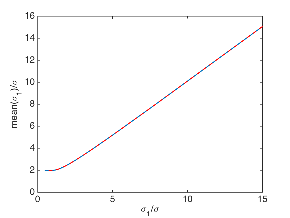
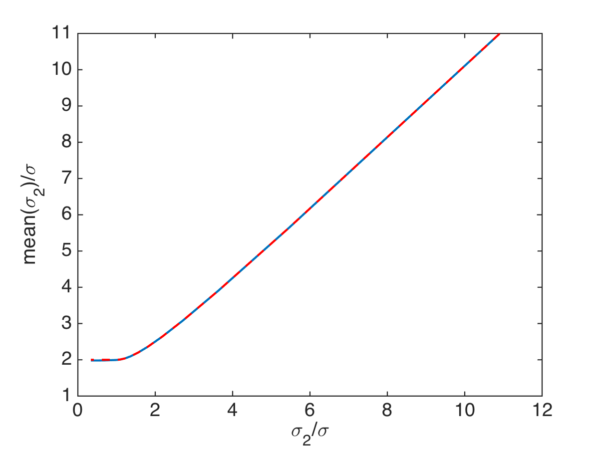
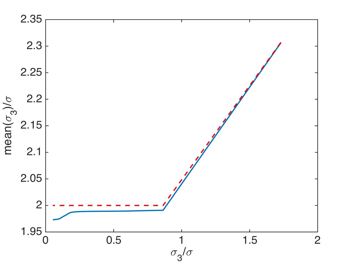
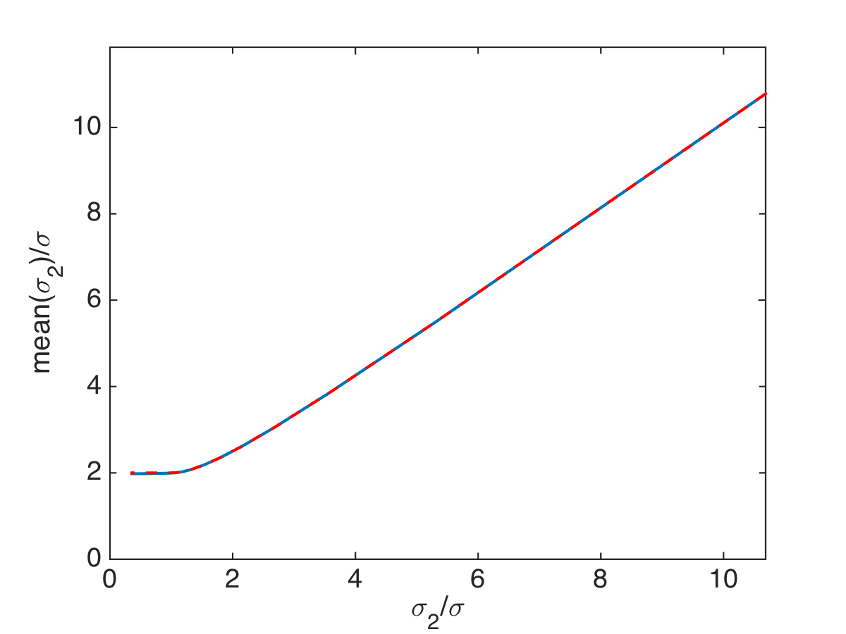
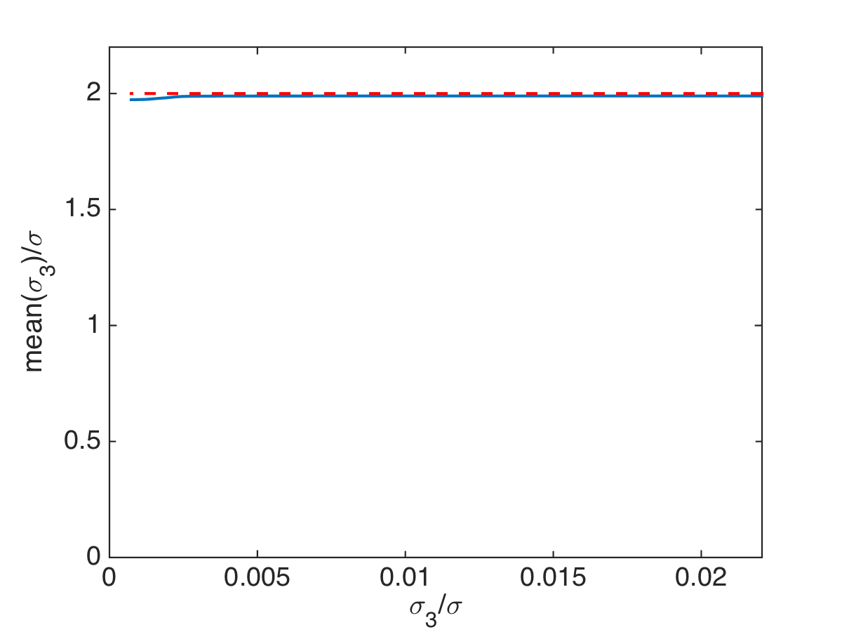
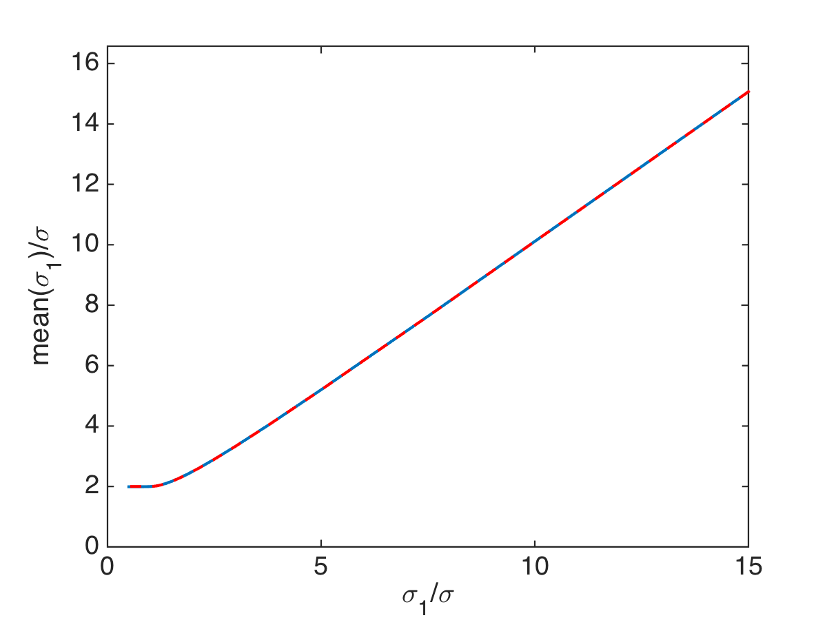
We plot with solid blue lines in Figure 2 the empirical means of the singular values σ~jsubscript~𝜎𝑗\widetilde{\sigma}_{j} of 𝐃~~𝐃\widetilde{{{\bf D}}}, for j=1,2,3𝑗123j=1,2,3 and σ(0,2σ1)𝜎02subscript𝜎1\sigma\in(0,2\sigma_{1}). The abscissa is σj/σsubscript𝜎𝑗𝜎\sigma_{j}/\sigma and the ordinate is mean[σ~j]/σmeandelimited-[]subscript~𝜎𝑗𝜎\mbox{mean}[\widetilde{\sigma}_{j}]/\sigma. The results are in excellent agreement with the asymptotic formulas

σ~j{σj(1+σ2/σj2)ifσj>σ,2σifσj<σ,subscript~𝜎𝑗casessubscript𝜎𝑗1superscript𝜎2superscriptsubscript𝜎𝑗2ifsubscript𝜎𝑗𝜎2𝜎ifsubscript𝜎𝑗𝜎\widetilde{\sigma}_{j}\approx\left\{\begin{array}[]{ll}\sigma_{j}\left(1+\sigma^{2}/\sigma_{j}^{2}\right)&\mbox{if}~{}\sigma_{j}>\sigma,\\ 2\sigma&\mbox{if}~{}\sigma_{j}<\sigma,\end{array}\right. (83)

plotted in the figure with dotted red lines. The top row in Figure 2 is for the large aperture regime and the bottom row for the small aperture regime. The plots are similar, except that in the small aperture case σ3subscript𝜎3\sigma_{3} cannot be distinguished from noise.
Refer to caption
Refer to caption
Refer to caption
Refer to caption
Refer to caption
Refer to caption
Fig. 2: Plots of mean[σ~j]/σmeandelimited-[]subscript~𝜎𝑗𝜎\mbox{mean}[\widetilde{\sigma}_{j}]/\sigma vs. σj/σsubscript𝜎𝑗𝜎\sigma_{j}/\sigma, for j=1,2,3𝑗123j=1,2,3. The empirical estimates of the means are shown with solid blue lines and the asymptotic estimates (83) are shown with dotted red lines. The top row is for the large aperture regime and the bottom row for the small aperture regime.
Refer to caption
Refer to caption
Refer to caption
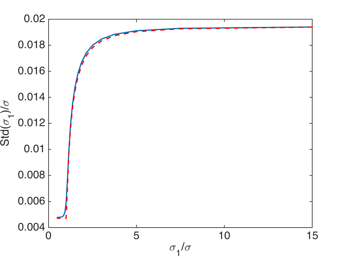
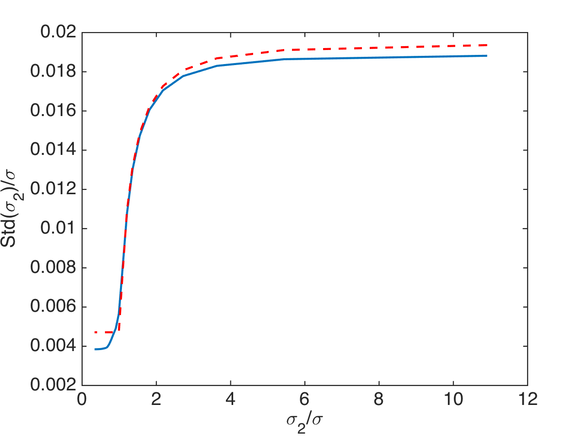
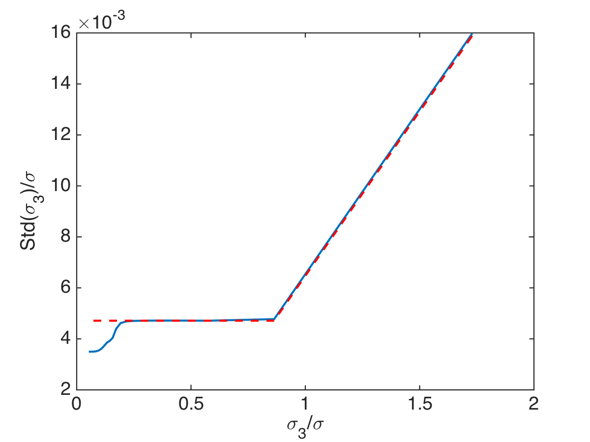
Fig. 3: Plots of std[σ~j]/σstddelimited-[]subscript~𝜎𝑗𝜎\mbox{std}[\widetilde{\sigma}_{j}]/\sigma vs. σj/σsubscript𝜎𝑗𝜎\sigma_{j}/\sigma, for j=1,2,3𝑗123j=1,2,3 in the large aperture regime. The empirical estimates are shown with solid blue lines and the asymptotic estimates (84) with dotted red lines.

In Figure 3 we plot the standard deviations of σ~jsubscript~𝜎𝑗\widetilde{\sigma}_{j} and note that they are much smaller than the means, so σ~jsubscript~𝜎𝑗\widetilde{\sigma}_{j} are approximately deterministic. We show the plots of std(σ~j)stdsubscript~𝜎𝑗\mbox{std}(\widetilde{\sigma}_{j}) in the large aperture regime, and compare them with the asymptotic ones in Theorem 1,

std(σ~j){σ(6N)1/2(1σ2/σj2)1/2ifσj>σ,σ(6N)2/30.813ifσj<σ.stdsubscript~𝜎𝑗cases𝜎superscript6𝑁12superscript1superscript𝜎2superscriptsubscript𝜎𝑗212ifsubscript𝜎𝑗𝜎𝜎superscript6𝑁230.813ifsubscript𝜎𝑗𝜎\mbox{std}(\widetilde{\sigma}_{j})\approx\left\{\begin{array}[]{ll}\frac{\sigma}{(6N)^{1/2}}(1-\sigma^{2}/\sigma_{j}^{2})^{1/2}&\mbox{if}~{}\sigma_{j}>\sigma,\\ \frac{\sigma}{(6N)^{2/3}}\sqrt{0.813}&\mbox{if}~{}\sigma_{j}<\sigma.\end{array}\right. (84)

Here we used that std(𝒵2)0.813.stdsubscript𝒵20.813\mbox{std}(\mathcal{Z}_{2})\approx\sqrt{0.813}. The results at small aperture are similar.
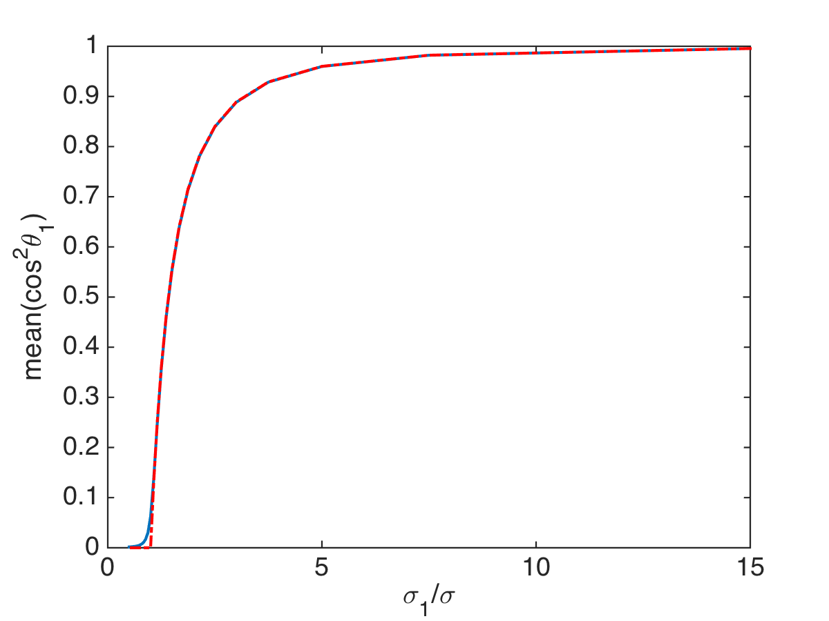
Refer to caption
Refer to caption
Fig. 4: Plots of mean[cos2θ1]meandelimited-[]superscript2subscript𝜃1\mbox{mean}[\cos^{2}\theta_{1}] (left) and std[cos2θ1]/mean[cos2θ1]stddelimited-[]superscript2subscript𝜃1meandelimited-[]superscript2subscript𝜃1\mbox{std}[\cos^{2}\theta_{1}]/\mbox{mean}[\cos^{2}\theta_{1}] (right) vs. σ1/σsubscript𝜎1𝜎\sigma_{1}/\sigma, in the large aperture regime. The empirical estimates are shown with solid blue lines and the asymptotic estimates (84) are plotted with dotted red lines.

In Figure 4 we display the empirical mean of cos2θ1=|u~1u1|2superscript2subscript𝜃1superscriptsubscript~u1subscriptu12\cos^{2}\theta_{1}=|\widetilde{\itbf u}_{1}{{\itbf u}}_{1}|^{2} and compare it with its asymptotic prediction (42). We also plot the standard deviation, and note that it is much smaller than the mean when σ1>σsubscript𝜎1𝜎\sigma_{1}>\sigma, as expected from Theorem 1. The plots look the same for the large and small aperture regimes, and for the other angles θ2subscript𝜃2\theta_{2} and θ3subscript𝜃3\theta_{3}, when σ2subscript𝜎2\sigma_{2} and σ3subscript𝜎3\sigma_{3} are greater than σ𝜎\sigma.

6.2.2 Incomplete measurements

We do not include plots for the incomplete measurements, where 𝐁=𝐃S𝐁subscript𝐃𝑆{\bf B}={{\bf D}}_{{}_{S}}, because they do not add much information. Instead, we display below the effect of the sensing matrix 𝐒𝐒{\bf S} on the singular values of 𝐃Ssubscript𝐃𝑆{{\bf D}}_{{}_{S}}. As explained in section 5, we expect that the inversion algorithm will be most effective when the effective rank ~~\widetilde{\mathfrak{R}} equals the rank =33\mathfrak{R}=3 of 𝐃Ssubscript𝐃𝑆{{\bf D}}_{{}_{S}}. Since ~~\widetilde{\mathfrak{R}} is the number of singular values of 𝐃Ssubscript𝐃𝑆{{\bf D}}_{{}_{S}} that are larger than 2σ2𝜎2\sigma, the more small singular values 𝐃Ssubscript𝐃𝑆{{\bf D}}_{{}_{S}} has, the worse the inversion results.

When 𝐒=(e1)𝐒subscripte1{\bf S}=(\vec{{{\itbf e}}}_{1}), the singular values of 𝐃~Ssubscript~𝐃𝑆\widetilde{{{\bf D}}}_{{}_{S}} are

σ1=1.099,σ2=0.087,σ3=0.007formulae-sequencesubscript𝜎11.099formulae-sequencesubscript𝜎20.087subscript𝜎30.007\sigma_{1}=1.099,~{}~{}\sigma_{2}=0.087,~{}~{}\sigma_{3}=0.007

in the large aperture regime and

σ1=0.015,σ2=1.7105,σ3=1.6108formulae-sequencesubscript𝜎10.015formulae-sequencesubscript𝜎21.7superscript105subscript𝜎31.6superscript108\sigma_{1}=0.015,~{}~{}\sigma_{2}=1.7\cdot 10^{-5},~{}~{}\sigma_{3}=1.6\cdot 10^{-8}

in the small aperture regime. The results are similar for 𝐒=(e2)𝐒subscripte2{\bf S}=(\vec{{{\itbf e}}}_{2}), and show that as predicted by the analysis in section 4.2, only one singular value is large. The case with 𝐒=(e3)𝐒subscripte3{\bf S}=(\vec{{{\itbf e}}}_{3}) is much worse, because all the singular values are small, and are likely to be dominated by noise. Explicitly, we get

σ1=0.145,σ2=0.065,σ3=0.023formulae-sequencesubscript𝜎10.145formulae-sequencesubscript𝜎20.065subscript𝜎30.023\sigma_{1}=0.145,~{}~{}\sigma_{2}=0.065,~{}~{}\sigma_{3}=0.023

in large aperture regime and

σ1=2.3105,σ2=1.3105,σ3=1.9107formulae-sequencesubscript𝜎12.3superscript105formulae-sequencesubscript𝜎21.3superscript105subscript𝜎31.9superscript107\sigma_{1}=2.3\cdot 10^{-5},~{}~{}\sigma_{2}=1.3\cdot 10^{-5},~{}~{}\sigma_{3}=1.9\cdot 10^{-7}

in the small aperture regime. Finally, when both cross-range components of the electric field are measured using 𝐒=(e1,e2)𝐒subscripte1subscripte2{\bf S}=(\vec{{{\itbf e}}}_{1},\vec{{{\itbf e}}}_{2}), the singular values of 𝐃Ssubscript𝐃𝑆{{\bf D}}_{{}_{S}} are similar to those of 𝐃𝐃{{\bf D}}. Thus, we expect inversion results which are comparable to those for complete measurements.

6.2.3 Estimation of the noise level

We display in Figure 5 the empirical mean and standard deviation of the unbiased estimate (47) of the noise level, using the complete measurement matrix 𝐃~~𝐃\widetilde{{{\bf D}}}. We note that σemean[σe]σ.superscript𝜎𝑒meandelimited-[]superscript𝜎𝑒𝜎\sigma^{e}\approx\mbox{mean}[\sigma^{e}]\approx\sigma. The estimate (48) is very similar, because we have many sensors. For the same reason we obtain similar estimates of σ𝜎\sigma from incomplete measurements. If the number of sensors were smaller, then the refined estimation methods proposed in [17] could be used.
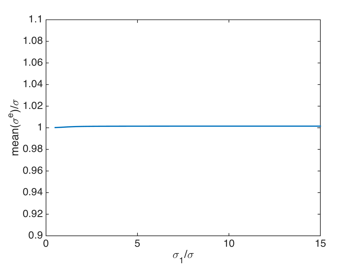
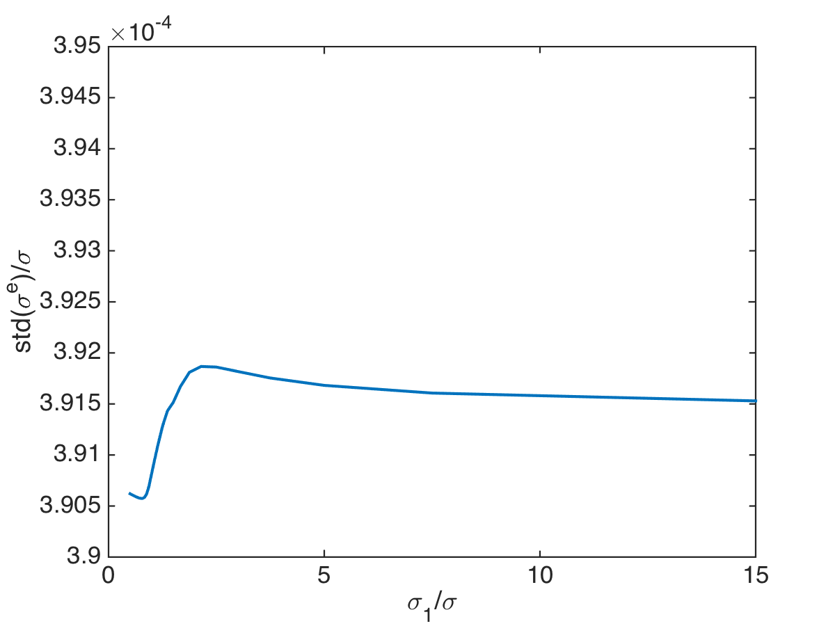
Refer to caption
Refer to caption
Fig. 5: Empirical mean of the noise level estimate (47) (left plot) and standard deviation (right plot). The results are normalized by σ𝜎\sigma. The abscissa is σ1/σsubscript𝜎1𝜎\sigma_{1}/\sigma.

6.3 Inversion results for one inclusion

We present results for the inclusion at y1=(λ,λ,L)subscripty1𝜆𝜆𝐿\vec{{{\itbf y}}}_{1}=(\lambda,-\lambda,L), with reflectivity tensor (81), in both the large and small aperture regimes. We compare the MUSIC method (53) with the imaging function (59), and estimate the reflectivity tensor as in section 5.3.
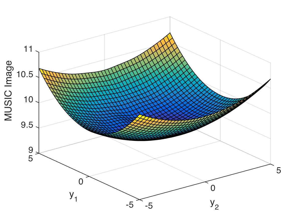
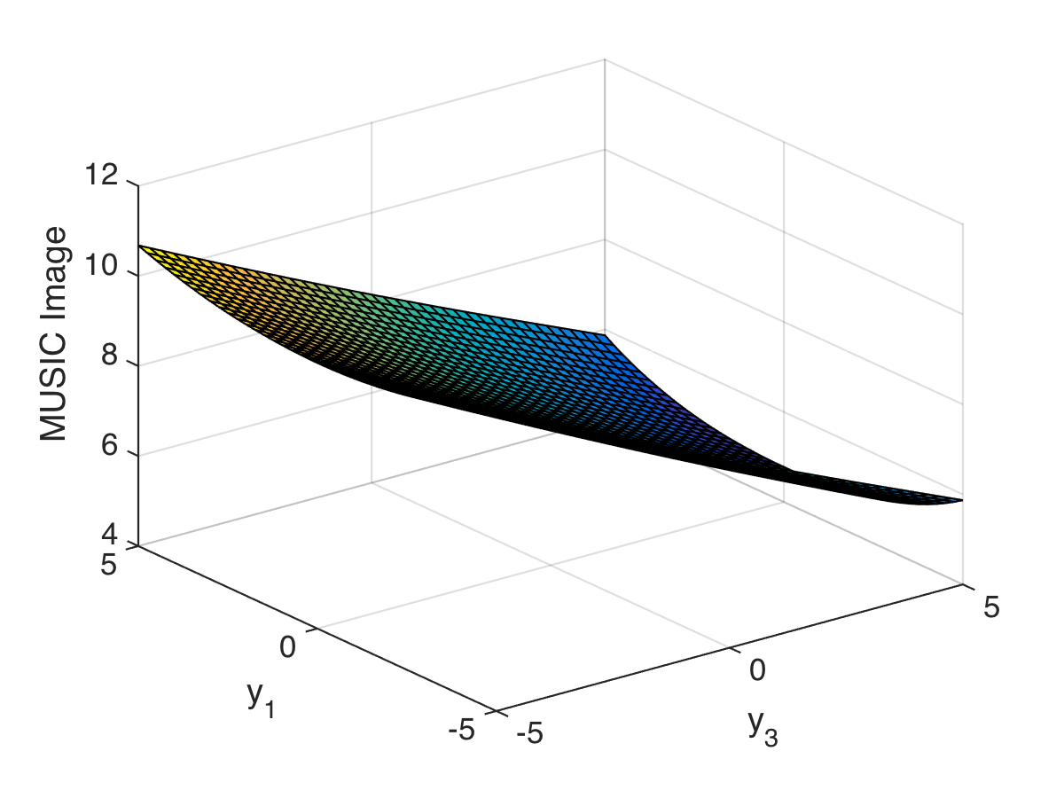
Refer to caption
Refer to caption
Refer to caption
Refer to caption
Fig. 6: MUSIC imaging of one inclusion in the large aperture regime and complete measurements. We display MUSIC(y)subscript𝑀𝑈𝑆𝐼𝐶y\mathcal{I}_{{}_{MUSIC}}(\vec{{{\itbf y}}}) in the plane y3=Lsubscript𝑦3𝐿y_{3}=L (left) and y2=λsubscript𝑦2𝜆y_{2}=-\lambda (right). The axes are in units of the wavelength. The top row is for 75%percent7575\% noise and the bottom row for 25%percent2525\%.

6.3.1 Complete measurements

Let us begin with Figure 6, which shows the surface plots of MUSIC(y)subscript𝑀𝑈𝑆𝐼𝐶y\mathcal{I}_{{}_{MUSIC}}(\vec{{{\itbf y}}}) in the planes y3=Lsubscript𝑦3𝐿y_{3}=L and y2=λsubscript𝑦2𝜆y_{2}=-\lambda, respectively. These are obtained in the large aperture regime, for two realizations of the noise matrix: one for 25%percent2525\% noise (bottom row) and the other for 75%percent7575\% noise (top row). At the higher noise level the MUSIC function fails to localize the inclusion, as it has no peak. For comparison, we display in Figure 7 the results obtained with our imaging function (59), for the same realization at 75%percent7575\% noise. We do not show the images for 25%percent2525\% noise because they are similar. The images are a significant improvement over those in Figure 6, and they clearly localize the inclusion in range and cross-range.
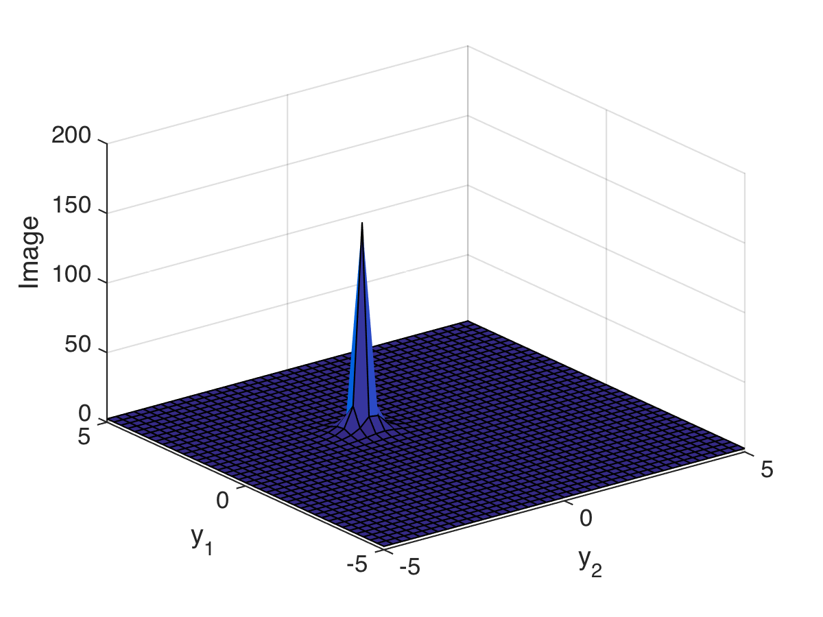
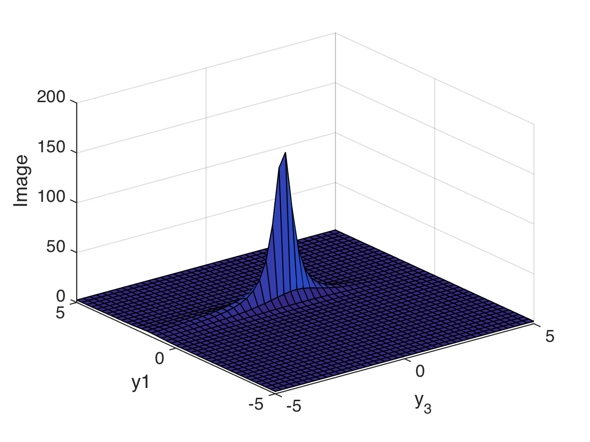
Refer to caption
Refer to caption
Fig. 7: Imaging function (59) in the large aperture regime, for complete measurements and 75%percent7575\% noise. We display (y)y\mathcal{I}(\vec{{{\itbf y}}}) in the plane y3=Lsubscript𝑦3𝐿y_{3}=L (left) and y2=λsubscript𝑦2𝜆y_{2}=-\lambda (right). The axes are in units of the wavelength.
Refer to caption
Refer to caption
Refer to caption
Refer to caption
Refer to caption
Refer to caption
Refer to caption
Refer to caption
Refer to caption
Fig. 8: The histograms of the peak location in y1subscript𝑦1y_{1} (top), y2subscript𝑦2y_{2} (middle) and y3subscript𝑦3y_{3} (bottom) of the imaging function (59) in the large aperture regime. The left column is for σ/σ1=75%𝜎subscript𝜎1percent75\sigma/\sigma_{1}=75\%, the middle column for 50%percent5050\% and the right column for 25%percent2525\%. The abscissa is in units of the wavelength.

To illustrate the statistical stability of our imaging function (59), we display in Figure 8 the histograms of the peak locations along the three coordinate axes, for one hundred realizations of the noise at 25%percent2525\%, 50%percent5050\% and 75%percent7575\% noise level. The effective rank of the noisy data matrix 𝐃~~𝐃\widetilde{{{\bf D}}} is ~=1~1\widetilde{\mathfrak{R}}=1 at 75%percent7575\% noise level and ~=2~2\widetilde{\mathfrak{R}}=2 for the weaker noise. We note that the focusing in cross-range is perfect for all realizations. The range focusing suffers slightly at the higher noise levels, but the error is at most 1.5λ1.5𝜆1.5\lambda.

Refer to caption
Refer to caption
Refer to caption
Refer to caption
Refer to caption
Refer to caption
Refer to caption
Refer to caption
Refer to caption
Fig. 9: The histograms of the peak location in y1subscript𝑦1y_{1} (top), y2subscript𝑦2y_{2} (middle) and y3subscript𝑦3y_{3} (bottom) of the imaging function (59) in the small aperture regime. The left column is for σ/σ1=50%𝜎subscript𝜎1percent50\sigma/\sigma_{1}=50\%, the middle column for 25%percent2525\% and the right column for 10%percent1010\%. The abscissa is in units of the wavelength.

Imaging is more difficult in the small aperture, as seen in Figure 9. Although the cross-range localization remains robust up to 50%percent5050\% noise, and the error is bounded by λ𝜆\lambda, which is an improvement over the resolution limit λL/a=10λ𝜆𝐿𝑎10𝜆\lambda L/a=10\lambda of migration imaging, the range localization fails even at 10%percent1010\% noise. This is because the effective rank of 𝐃~~𝐃\widetilde{{{\bf D}}} is ~=2~2\widetilde{\mathfrak{R}}=2 for all the simulations in Figure 9, and as explained in section 5.3.1, the projection matrices on the subspace spanned by the first two singular vectors are approximately independent of the range of the inclusion. To determine the range we need an array of larger aperture, or two arrays that view the inclusion from different directions. Alternatively, we may probe the medium with broad-band pulses and estimate the range from travel times of the scattered returns.
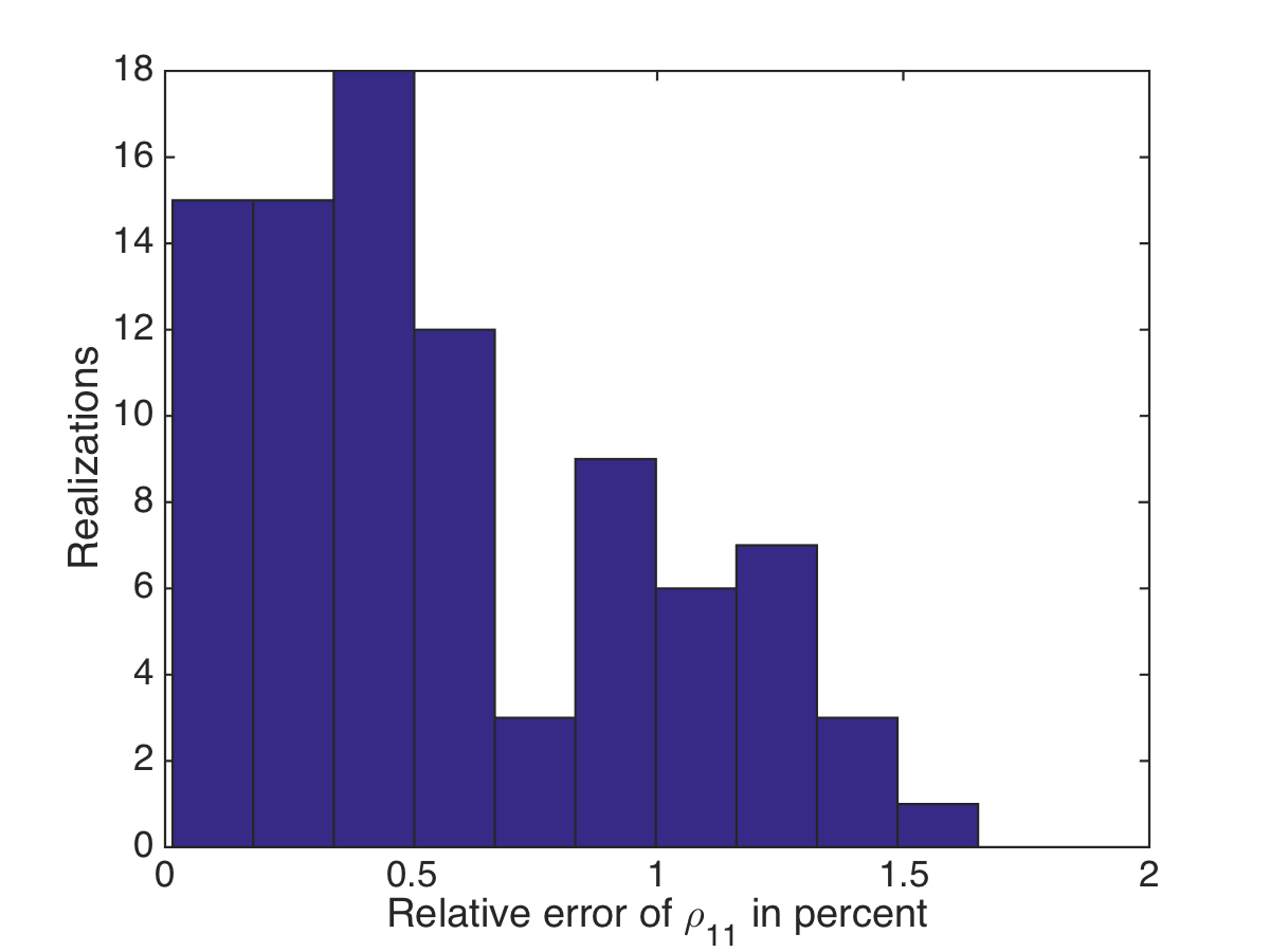
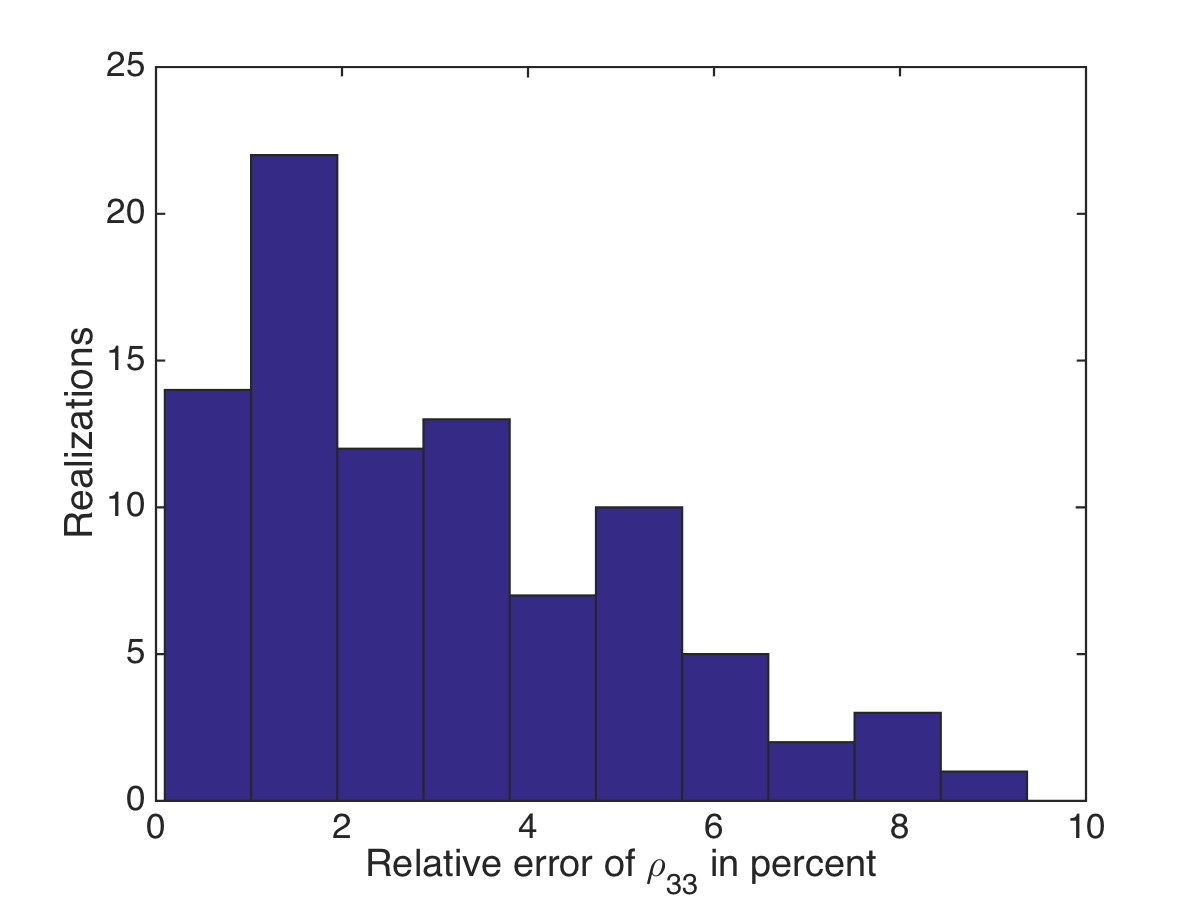
Refer to caption
Refer to caption
Refer to caption
Refer to caption
Refer to caption
Refer to caption
Fig. 10: Histograms of the relative errors of the components ρ11subscript𝜌11\rho_{11} (left), ρ33subscript𝜌33\rho_{33} (middle) and ρ13subscript𝜌13\rho_{13} (right) of the reflectivity tensor 𝝆𝝆\bm{\rho}, for the large aperture regime and complete measurements at 25%percent2525\% noise (top row) and 50%percent5050\% noise (bottom row). The abscissa is in percent.

The histograms of the relative errors in the estimation of the reflectivity tensor are displayed in Figures 10, for the large aperture regime and at 25%percent2525\% and 50%percent5050\% noise levels. The estimates are obtained using equations (70) and (72), and the peak location of the imaging function (59). The plots in the left column are for ρ11subscript𝜌11\rho_{11}, in the middle column for ρ33subscript𝜌33\rho_{33}, and in the right column for ρ13subscript𝜌13\rho_{13}. The results for ρ22subscript𝜌22\rho_{22} and ρ12subscript𝜌12\rho_{12} are similar to those for ρ11subscript𝜌11\rho_{11}, and the results for ρ23subscript𝜌23\rho_{23} are similar to those for ρ13subscript𝜌13\rho_{13}. We note that the errors are below 10%percent1010\% at 25%percent2525\% noise and naturally, they increase with the noise level. As expected, the errors are larger for ρ33subscript𝜌33\rho_{33} and ρ13subscript𝜌13\rho_{13}, but not by a big factor. This is because the condition number of the search matrix 𝓖(y)𝓖y\bm{\mathcal{G}}(\vec{{{\itbf y}}}), defined as the ratio of its largest and smallest singular values, equals 2.62.62.6 in the large aperture regime. The estimates are worse in the small aperture regime, where the condition number of 𝓖(y)𝓖y\bm{\mathcal{G}}(\vec{{{\itbf y}}}) is 23.323.323.3, as shown in Figure 11. Here we also have errors due to the poor estimates of the range component of the inclusion location.
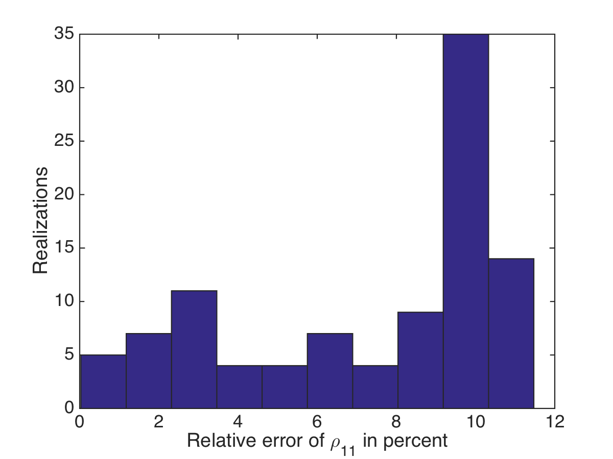
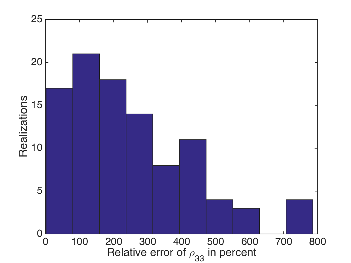
Refer to caption
Refer to caption
Refer to caption
Fig. 11: Histograms of the relative errors of the components ρ11subscript𝜌11\rho_{11} (left), ρ33subscript𝜌33\rho_{33} (middle) and ρ13subscript𝜌13\rho_{13} (right) of the reflectivity tensor 𝝆𝝆\bm{\rho}, for the small aperture regime and complete measurements at 25%percent2525\% noise. The abscissa is in percent.

6.3.2 Incomplete measurements

If the sensors measure a single component of the scattered electric field, say along eqsubscripte𝑞\vec{{{\itbf e}}}_{q}, the best choice is for q=1𝑞1q=1 or 222. The inversion results are very poor when q=3𝑞3q=3, even at low levels of noise, as expected from the discussion in section 4.2. We show here results for the sensing matrix 𝐒=(e1)𝐒subscripte1{\bf S}=(\vec{{{\itbf e}}}_{1}), in the large aperture regime, and compare them with those in Figures 8 and 10. We do not show results in the small aperture regime because they do not add more information, and they are, as expected, worse than in the large aperture regime.
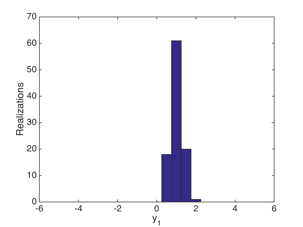
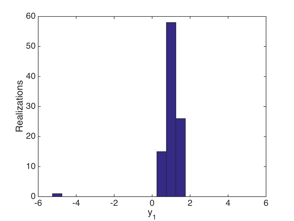
Refer to caption
Refer to caption
Refer to caption
Refer to caption
Refer to caption
Refer to caption
Refer to caption
Refer to caption
Refer to caption
Fig. 12: The histograms of the peak location in y1subscript𝑦1y_{1} (top), y2subscript𝑦2y_{2} (middle) and y3subscript𝑦3y_{3} (bottom) of the imaging function (59), in the large aperture regime, for incomplete measuremenst with 𝐒=(e1)𝐒subscripte1{\bf S}=(\vec{{{\itbf e}}}_{1}). The left column is for σ/σ1=75%𝜎subscript𝜎1percent75\sigma/\sigma_{1}=75\%, the middle column for 50%percent5050\% and the right column for 25%percent2525\%. The abscissa is in units of the wavelength.

The histogram plots in Figure 12 show that the inclusion localization is worse than in the complete measurement case (Figure 8), but not dramatically so. However, the errors in the estimation of the reflectivity tensor are much larger, even at the 25%percent2525\% noise level. Compare the results in Figure 13 to those on the top row of Figure 10. This demonstrates the benefit of measuring more than one component of the scattered electric field.

We do not display inversion results from incomplete data with the sensing matrix 𝐒=(e1,e2)𝐒subscripte1subscripte2{\bf S}=(\vec{{{\itbf e}}}_{1},\vec{{{\itbf e}}}_{2}), because they are comparable to those in the complete measurements case. This is expected from the discussion in section 4.2.
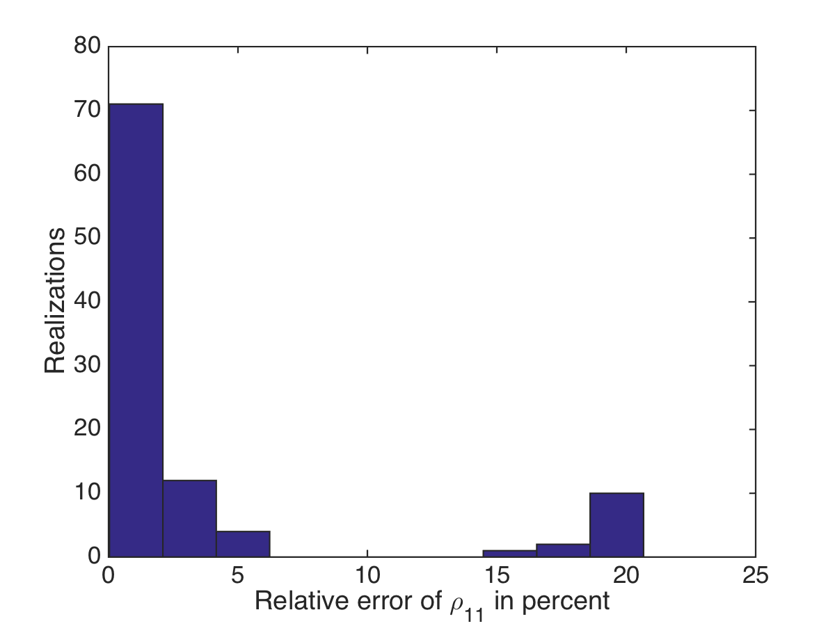
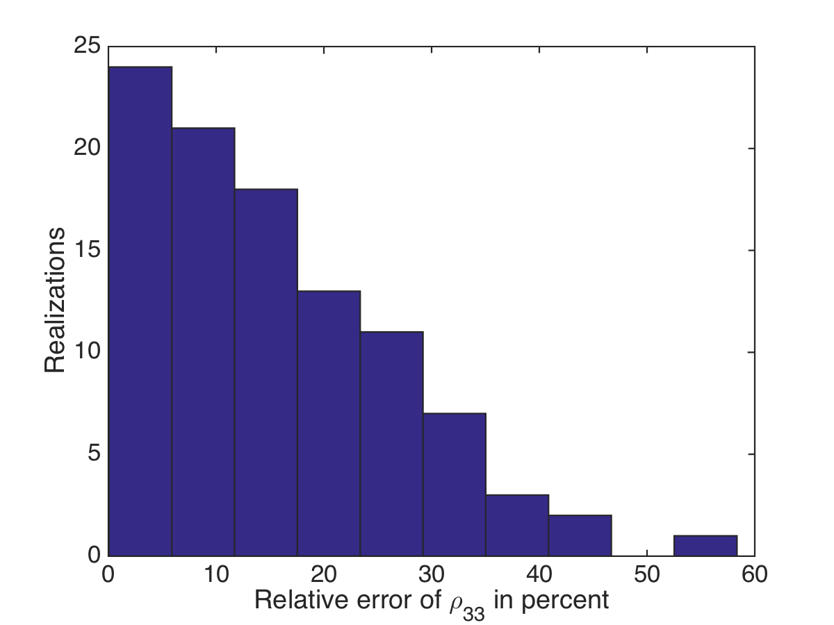
Refer to caption
Refer to caption
Refer to caption
Fig. 13: Histograms of the relative errors of the components ρ11subscript𝜌11\rho_{11} (left), ρ33subscript𝜌33\rho_{33} (middle) and ρ13subscript𝜌13\rho_{13} (right) of the reflectivity tensor 𝝆𝝆\bm{\rho}, in the large aperture regime, for incomplete measuremenst with 𝐒=(e1)𝐒subscripte1{\bf S}=(\vec{{{\itbf e}}}_{1}) and 25%percent2525\% noise. The abscissa is in percent.
Refer to caption
Refer to caption
Fig. 14: Image of three inclusions in the large aperture regime, for complete measurements and 25%percent2525\% noise (left) and 75%percent7575\% noise (right). The display is in the plane y3=Lsubscript𝑦3𝐿y_{3}=L. The axes are in units of the wavelength. The locations of the inclusions are indicated with red circles.

6.4 Inversion results for multiple inclusions

We present results for three inclusions at y1=(λ,λ,L)subscripty1𝜆𝜆𝐿\vec{{{\itbf y}}}_{1}=(\lambda,-\lambda,L), y2=(10λ,6λ,L)subscripty210𝜆6𝜆𝐿\vec{{{\itbf y}}}_{2}=(-10\lambda,6\lambda,L) and y3=(5λ,4λ,L)subscripty35𝜆4𝜆𝐿\vec{{{\itbf y}}}_{3}=(5\lambda,4\lambda,L). They are localized using the imaging function (67), and their reflectivities are estimated as in (72). The first inclusion has the reflectivity (81) and for the other two we have

α3𝝆2=(91.1229.4312.0429.4369.998.5312.048.53111.60).superscript𝛼3subscript𝝆2matrix91.1229.4312.0429.4369.998.5312.048.53111.60\alpha^{-3}\bm{\rho}_{2}=\left(\begin{matrix}91.12&-29.43&-12.04\\ -29.43&69.99&-8.53\\ -12.04&-8.53&111.60\end{matrix}\right). (85)

and

α3𝝆3=(99.375.3526.895.35101.1210.3726.8910.37137.06).superscript𝛼3subscript𝝆3matrix99.375.3526.895.35101.1210.3726.8910.37137.06\alpha^{-3}\bm{\rho}_{3}=\left(\begin{matrix}99.37&5.35&-26.89\\ 5.35&101.12&-10.37\\ -26.89&-10.37&137.06\end{matrix}\right). (86)

In the large aperture regime the matrix 𝐃𝐃{{\bf D}} has rank =99\mathfrak{R}=9, and singular values

1.76=σ1>σ2>>σ5=1.14,0.57=σ6>σ7>σ8=0.18,σ9=0.07.formulae-sequence1.76subscript𝜎1subscript𝜎2subscript𝜎51.140.57subscript𝜎6subscript𝜎7subscript𝜎80.18subscript𝜎90.071.76=\sigma_{1}>\sigma_{2}>\ldots>\sigma_{5}=1.14,~{}~{}0.57=\sigma_{6}>\sigma_{7}>\sigma_{8}=0.18,~{}~{}\sigma_{9}=0.07.

The rank of 𝐃𝐃{{\bf D}} is still nine in the small aperture case, but the matrix has three very small singular values that are indistinguishable from noise at levels as small as 1%percent11\%.

0.034=σ1>σ2>>σ6=0.012,6.39105=σ7>σ8>σ9=2.12105.formulae-sequence0.034subscript𝜎1subscript𝜎2subscript𝜎60.0126.39superscript105subscript𝜎7subscript𝜎8subscript𝜎92.12superscript1050.034=\sigma_{1}>\sigma_{2}>\ldots>\sigma_{6}=0.012,~{}~{}6.39\cdot 10^{-5}=\sigma_{7}>\sigma_{8}>\sigma_{9}=2.12\cdot 10^{-5}.

For brevity we present only results in the complete measurement case, and a few realizations of the noise. The histograms of the estimated peak locations and of the errors in the estimation of the reflectivities are similar to those in the previous section.
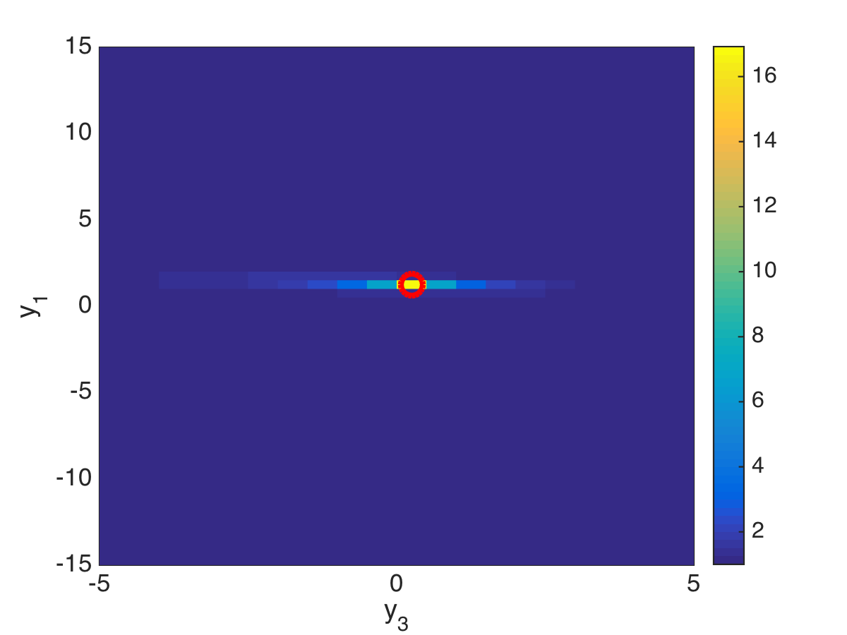
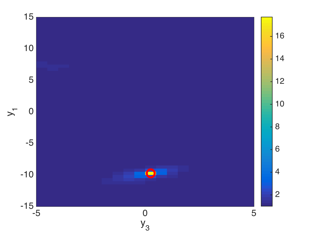
Refer to caption
Refer to caption
Refer to caption
Refer to caption
Refer to caption
Refer to caption
Fig. 15: Image of three inclusions in the large aperture regime, for complete measurements and 25%percent2525\% noise (top) and 75%percent7575\% noise (bottom). The displays are in the planes y2=yp,2subscript𝑦2subscript𝑦𝑝2y_{2}=y_{p,2}, for p=1,2,3𝑝123p=1,2,3. The axes are in units of the wavelength.

6.4.1 Large aperture regime

We display in Figure 14 the imaging function (67) in the plane y3=Lsubscript𝑦3𝐿y_{3}=L. The image on the left is for data with 25%percent2525\% noise, where the effective rank of 𝐃~~𝐃\widetilde{{{\bf D}}} is ~=6~6\widetilde{\mathfrak{R}}=6. The right image is for 75%percent7575\% noise, where the effective rank decreases to ~=3~3\widetilde{\mathfrak{R}}=3. The exact locations of the inclusions are indicated with red circles, and they coincide with the peaks of the imaging function. As expected, the peaks are more prominent when ~~\widetilde{\mathfrak{R}} is closer to \mathfrak{R} i.e., for the weaker noise. Note in particular that the inclusion at y2subscripty2\vec{{{\itbf y}}}_{2} is barely visible at the 75%percent7575\% noise level, because the singular vector h1(y2)subscripth1subscripty2{{\itbf h}}_{1}(\vec{{{\itbf y}}}_{2}) of 𝓖(y2)𝓖subscripty2\bm{\mathcal{G}}(\vec{{{\itbf y}}}_{2}) has a small projection on span{u1,u2,u3}spansubscriptu1subscriptu2subscriptu3\mbox{span}\{{{\itbf u}}_{1},{{\itbf u}}_{2},{{\itbf u}}_{3}\}. The images in Figure 15 tell a similar story. They are displayed in the planes y2=yp,2subscript𝑦2subscript𝑦𝑝2y_{2}=y_{p,2} for p=1,2,3𝑝123p=1,2,3, and show that the range resolution is worse than that in cross-range, specially at the higher noise level. Moreover, consistent with Figure 14, the inclusion at y2subscripty2\vec{{{\itbf y}}}_{2} is difficult to localize at 75%percent7575\% noise.

We present in Table 1 the relative errors (in percent) of the estimation (72) of the components of the reflectivities 𝝆psubscript𝝆𝑝\bm{\rho}_{p}, for p=1,2,3𝑝123p=1,2,3. Because the inclusions are well localized, the errors of 𝝆psubscript𝝆𝑝\bm{\rho}_{p} are of the form (69), and are mostly due to the noise. The interaction between the inclusions is negligible, as seen from the very accurate results at zero noise level. This is expected because the inclusions are further apart than λL/a=λ𝜆𝐿𝑎𝜆\lambda L/a=\lambda. The errors increase with the noise, but they remain small for some components, mainly on the diagonal of the reflectivity tensors.

ρ11subscript𝜌11\rho_{11} ρ22subscript𝜌22\rho_{22} ρ33subscript𝜌33\rho_{33} ρ12subscript𝜌12\rho_{12} ρ13subscript𝜌13\rho_{13} ρ33subscript𝜌33\rho_{33}
Inclusion 1 0.01 0.02 0.1 0.03 0.06 0.08
0%percent00\% noise Inclusion 2 0.2 0.3 0.3 0.7 1.9 2.9
Inclusion 3 0.03 0.02 0.04 0.3 0.1 0.2
Inclusion 1 0.6 0.5 1 4.9 3.8 5.0
25%percent2525\% noise Inclusion 2 3.7 5.1 2.4 10.7 19.3 44.7
Inclusion 3 2.9 1.2 7.7 48.0 21.7 21.7
Inclusion 1 3.3 1.8 5.7 7.1 31.3 9.9
75%percent7575\% noise Inclusion 2 7.4 5.2 8.9 4.7 34.7 98.3
Inclusion 3 2.1 0.7 7.4 45.2 18.1 49.4
Table 1: Table of relative errors (in percent) of the estimated components of the reflectivity tensors in the large aperture regime.
Refer to caption
Refer to caption
Fig. 16: Image of three inclusions in the large aperture regime, for complete measurements and 25%percent2525\% noise (left) and 50%percent5050\% noise (right). The display is in the plane y3=Lsubscript𝑦3𝐿y_{3}=L. The axes are in units of the wavelength. The locations of the inclusions are indicated with red circles.

6.4.2 Small aperture regime

As we saw in the previous section, imaging is more difficult in the small aperture regime. Range localization is impossible even at small levels of noise. Moreover, the resolution of the left image in Figure 16, obtained at 25%percent2525\% noise, is worse than that in Figure 14. The inclusions interact in this case, because they are separated by smaller distances than λL/a=10λ𝜆𝐿𝑎10𝜆\lambda L/a=10\lambda, and this adds to the difficulty. The right image in Figure 16 shows that one inclusion is obscured at 50%percent5050\% noise.

We do not show the errors in the estimation of the reflectivity tensor because they are bad even at small noise levels, due to the poor conditioning of the matrix 𝚺(y)𝚺y\bm{\Sigma}(\vec{{{\itbf y}}}) in (73), and the interaction of the inclusions.

7 Summary

We introduced and analyzed a robust methodology for detection, localization, and characterization of small electromagnetic inclusions from measurements of the time-harmonic electric field corrupted by additive noise. The methodology is motivated by the statistical analysis of the noisy data matrix gathered by an array of sensors. In particular, it uses random matrix theory results about low rank perturbations of large random matrices. The detection of the inclusions is carried out by the inspection of the top singular values of the data matrix. The localization is done with an imaging function that uses the predictable angles between the singular vectors of the noisy data matrix and of the noiseless matrix. The characterization of the inclusions amounts to estimating their reflectivity tensor which depends on the shape of their support and their electric permittivity.

The inversion methodology is robust with respect to a significant level of additive noise, much more than standard imaging methods like MUSIC can handle. We clarify that MUSIC localization fails because the singular vectors of the noisy data matrix are not collinear to those of the unperturbed matrix. A main result of the paper is that the angles between these singular vectors can be predicted and used to obtain a robust inclusion localization. We also explain that the resolution and stability of inversion are dependent on each other, and quantify the stability gain due to larger array aperture and more than one component of the electric field being recorded and processed.

Acknowledgements

Liliana Borcea’s work was partially supported by AFOSR Grant FA9550-15-1-0118.

References

  • [1] R. Alonso, L. Borcea, G. Papanicolaou, and C. Tsogka, Detection and imaging in strongly backscattering randomly layered media, Inverse Problems, 27 (2011), p. 025004.
  • [2] H. Ammari, J. Garnier, and V. Jugnon, Detection, reconstruction, and characterization algorithms in wave sensor imaging, Discrete and Continuous Dynamical Systems – Series S, 8 (2015), pp. 389–417.
  • [3] H. Ammari, J. Garnier, H. Kang, W.-K. Park, and K. Sølna, Imaging schemes for perfectly conducting cracks, SIAM Journal on Applied Mathematics, 71 (2011), pp. 68–91.
  • [4] H. Ammari, J. Garnier, and K. Sølna, A statistical approach to target detection and localization in the presence of noise, Waves in Random and Complex Media, 22 (2012), pp. 40–65.
  • [5] H. Ammari, E. Iakovleva, D. Lesselier, and G. Perrusson, MUSIC-type electromagnetic imaging of a collection of small three-dimensional inclusions, SIAM Journal on Scientific Computing, 29 (2007), pp. 674–709.
  • [6] A. Aubry and A. Derode, Detection and imaging in a random medium: A matrix method to overcome multiple scattering and aberration, Journal of Applied Physics, 106 (2009), p. 044903.
  • [7] A. B. Baggeroer, W. Kuperman, P. N. Mikhalevsky, et al., An overview of matched field methods in ocean acoustics, IEEE Journal of Oceanic Engineering, 18 (1993), pp. 401–424.
  • [8] J. Baik, G. Ben Arous, and S. Péché, Phase transition of the largest eigenvalue for nonnull complex sample covariance matrices, Annals of Probability, 33 (2005), pp. 1643–1697.
  • [9] J. Baik, R. Buckingham, and J. DiFranco, Asymptotics of Tracy-Widom distributions and the total integral of a Painlevé II function, Communications in Mathematical Physics, 280 (2008), pp. 463–497.
  • [10] F. Benaych-Georges and R. R. Nadakuditi, The eigenvalues and eigenvectors of finite, low rank perturbations of large random matrices, Advances in Mathematics, 227 (2011), pp. 494–521.
  • [11] B. Biondi, 3D seismic imaging, vol. 14, Society of Exploration Geophysicists, Tulsa, 2006.
  • [12] F. Cakoni, D. Colton, and P. Monk, The linear sampling method in inverse electromagnetic scattering, vol. 80 of CBMS-NSF Regional Conference Series in Applied Mathematics, SIAM, Philadelphia, 2011.
  • [13] M. Capitaine, C. Donati-Martin, D. Féral, et al., Central limit theorems for eigenvalues of deformations of Wigner matrices, Annales de l’Institut Henri Poincaré, Probabilités et Statistiques, 48 (2012), pp. 107–133.
  • [14] M. Cheney and B. Borden, Fundamentals of radar imaging, vol. 79, SIAM, Philadelphia, 2009.
  • [15] A. J. Devaney, Super-resolution processing of multi-static data using time reversal and music, tech. report, Northeastern University Report, 2000.
  • [16] A. C. Fannjiang, The MUSIC algorithm for sparse objects: a compressed sensing analysis, Inverse Problems, 27 (2011), p. 035013.
  • [17] J. Garnier and K. Sølna, Applications of random matrix theory for sensor array imaging with measurement noise, in Random Matrix Theory, Interacting Particle Systems, and Integrable Systems, Cambridge University Press, Cambridge, 2014, pp. 223–246.
  • [18] J. Hadamard, Résolution d’une question relative aux déterminants, Bull. Sci. Math, 17 (1893), pp. 240–246.
  • [19] I. M. Johnstone, On the distribution of the largest eigenvalue in principal components analysis, Annals of Statistics, 29 (2001), pp. 295–327.
  • [20] A. Kirsch and N. Grinberg, The factorization method for inverse problems, Oxford University Press, Oxford, 2008.
  • [21] V. A. Marchenko and L. A. Pastur, Distribution of eigenvalues for some sets of random matrices, Matematicheskii Sbornik, 114 (1967), pp. 507–536.
  • [22] R. O. Schmidt, Multiple emitter location and signal parameter estimation, IEEE Transactions on Antennas and Propagation, 34 (1986), pp. 276–280.
  • [23] A. Sihvola and I. Lindell, Polarizability modeling of heterogeneous media, Progress in Electromagnetics Research (PIER 6), Dielectric Properties of Heterogeneous Materials, Priou, A.(ed.), Elsevier, Amsterdam, (1992). http://ww.jpier.org/PIER/pier06/03.900105.pdf.