Distributed Multi-Task Learning with Shared Representation

Abstract

We study the problem of distributed multi-task learning with shared representation, where each machine aims to learn a separate, but related, task in an unknown shared low-dimensional subspaces, i.e. when the predictor matrix has low rank. We consider a setting where each task is handled by a different machine, with samples for the task available locally on the machine, and study communication-efficient methods for exploiting the shared structure.

1 Introduction

Multi-task learning is widely used learning framework in which similar tasks are considered jointly for the purpose of improving performance compared to learning the tasks separately [13]. By transferring information between related tasks it is hoped that samples will be better utilized, leading to improved generalization performance. Multi-task learning has been successfully applied, for example, in natural language understanding [15], speech recognition [32], remote sensing [44], image classification [25], spam filtering [43], web search [14], disease prediction [49], and eQTL mapping [23] among other applications.

Here, we study multi-task learning in a distributed setting, where each task is handled by a different machine and communication between machines is expensive. That is, each machine has access to data for a different task and needs to learn a predictor for that task, where machines communicate with each other in order to leverage the relationship between the tasks. This situation lies between a homogeneous distributed learning setting [e.g. 36], where all machines have data from the same source distribution, and inhomogeneous consensus problems [e.g. 30, 11, 6] where the goal is to reach a single consensus predictor or iterate which is the same on all machines. The main argument for this setting is that if each machine indeed has access to different data (e.g. from a different geographical region or different types of users), as in the consensus problems studied by Balcan et al. [6], then we should allow a different predictor for each distribution, instead of insisting on a single consensus predictor, while still trying to leverage the relationship and similarity between data distributions, as in classical multi-task learning. As was recently pointed out by Wang et al. [41], allowing separate predictors for each task instead of insisting on a consensus predictor changes the fundamental nature of the distributed learning problem, allows for different optimization methods, and necessitates a different analysis approach, more similar to homogeneous distributed learning as studied by Shamir and Srebro [36].

The success of multi-task learning relies on the relatedness between tasks. While Wang et al. [41] studied tasks related through shared sparsity, here we turn to a more general, powerful and empirically more successful model of relatedness, where the predictors for different tasks lie in some (a-priori unknown) shared low-dimensional subspace and so the matrix of predictors is of low rank [3, 2, 45, 4]. In a shared sparsity model, information from all tasks is used to learn a subset of the input features which are then used by all tasks. In contrast, in a shared subspace model, novel features, which are linear functions of the input features, are learned. The model can thus be viewed as a two-layer neural network, with the bottom layer learned jointly across tasks and the top layer task-specific. Being arguably the most complex multi-layer network that we can fully analyze, studying such models can also serve as a gateway to using deeper networks for learning shared representations.

Multi-task learning with a shared subspace is well-studied in a centralized setting, where data for all tasks are on the same machine, and some global centralized procedure is used to find a good predictor for each task. In such a situation, nuclear norm regularization is often used to leverage the low rank structure [e.g. 4, 2] and learning guarantees are known ([28] and see also Section 2). With the growth of modern massive data sets, where tasks and data often too big to handle on a single machine, it is important to develop methods also for the distributed setting. Unfortunately, the distributed multi-task setting is largely unexplored and we are not aware of any prior for on distributed multi-task learning with shared subspaces.

In this paper we focus on methods with efficient communication complexity (i.e. with as small as possible communication between machines), that can still leverage most of the statistical benefit of shared-subspace multi-task learning. Although all our methods are also computationally tractable and can be implemented efficiently, we are less concerned here with minimizing the runtime on each machine separately, considering communication, instead, as the main bottleneck and the main resource to be minimized [8]. This is similar to the focus in distributed optimization approaches such as ADMM [11] and DANE [37] where optimization within each machine is taken as an atomic step.

Approach	Samples	Rounds	Communication	Worker Comp.	Master Comp.
Local	$\frac{A^{2}}{\varepsilon^{2}}$	$1$	$0$	ERM	$0$
Centralize	$\frac{A^{2}}{\epsilon^{2}}\left(\frac{r}{m}+\frac{r}{\widetilde{p}}\right)$	$1$	$\frac{A^{2}}{\epsilon^{2}}\left(\frac{r}{m}+\frac{r}{\widetilde{p}}\right)$	$0$	Nuclear Norm Minimization
ProxGD	$\frac{A^{2}}{\epsilon^{2}}\left(\frac{r}{m}+\frac{r}{\widetilde{p}}\right)$	$\frac{mHA^{2}}{\varepsilon}$	$2\cdot p$	Gradient Comp.	SV Shrinkage
AccProxGD	$\frac{A^{2}}{\epsilon^{2}}\left(\frac{r}{m}+\frac{r}{\widetilde{p}}\right)$	$\sqrt{\frac{mHA^{2}}{\varepsilon}}$	$2\cdot p$	Gradient Comp.	SV Shrinkage
ADMM	$\frac{A^{2}}{\epsilon^{2}}\left(\frac{r}{m}+\frac{r}{\widetilde{p}}\right)$	$\frac{mA^{2}}{\varepsilon}$	$3\cdot p$	ERM	SV Shrinkage
DFW	$\frac{A^{2}}{\epsilon^{2}}\left(\frac{r}{m}+\frac{r}{\widetilde{p}}\right)$	$\frac{mHA^{2}}{\varepsilon}$	$2\cdot p$	Gradient Comp.	Leading SV Comp.
DGSP	$-$	$\frac{mHA^{2}}{\varepsilon}$	$2\cdot p$	ERM	Leading SV Comp.
DNSP	$-$	$-$	$2\cdot p$	ERM	Leading SV Comp.

Table 1: Summary of resources required by different approaches to distributed multi-task learning with shared representations (for squared loss), in units of vector operations/communications, ignoring log-factors.

Contribution

The main contributions of this article are:

• Present and formalize the shared-subspace multi-task learning [4] in the novel distributed multitask setting, identifying the relevant problems and possible approaches. We analyze two baselines, several representative first-order distributed optimization methods, with careful sample and communication complexity analysis.

• We proposed and analyzed two subspace pursuit approaches which learns the shared representation in a greedy fashion, which leverage the low-dimensional predictive structure in a communication efficient way.

• We conducted comprehensive experimental comparisons of the discussed approaches on both simulated and real datasets, where we demonstrated that the proposed approaches are more communication efficient than first-order convex optimization methods.

Table 1 summarized the approaches studied in this paper, which will be discussed in detail in the following sections.

Homogeneous, Inhomogeneous and Multi-Task Distributed Learning.

We briefly review the relationship between homogeneous, inhomogeneous and multi-task learning, as recently presented by Wang et al. [41].

A typical situation considered in the literature is one in which data on different machines are all drawn i.i.d from the same source distribution. In this setting, tasks on different machines are all the same, which should be taken advantage of in optimization [37]. Furthermore, as each machine has access to samples from the source distribution it can perform computations locally, without ever communicating with other machines. While having zero communication cost, this approach does not compare favorably with the centralized approach, in which all data are communicated to the central machine and used to obtain one predictor, when measured in terms of statistical efficiency. The goal in this setting is to obtain performance close to that of the centralized approach, using the same number of samples, but with low communication and computation costs [36, 20, 48, 47, 26]. Another setting considered in the distributed optimization literature is that of consensus optimization. Here each machine has data from a different distribution and the goal is to find one vector of coefficients that is good for all the separate learning or optimization problems [11, 30, 6]. The difficulty of consensus problems is that the local objectives might be rather different, and, as a result, one can obtain lower bounds on the amount of communication that must be exchanged in order to reach a joint optimum.

In this paper we suggest a novel setting that combines aspects of the above two settings. On one hand, we assume that each machine has a different source distributions $\mathcal{D}_{j}$, corresponding to a different task, as in consensus problems. For example, each machine serves a different geographical location, or each is at a different hospital or school with different characteristics. But if indeed there are differences between the source distributions, it is natural to learn different predictors $\mathbf{w}_{j}$ for each machine, so that $\mathbf{w}_{j}$ is good for the distribution typical to that machine. In this regard, our distributed multi-task learning problem is more similar to single-source problems, in that machines could potentially learn on their own given enough samples and enough time. Furthermore, availability of other machines just makes the problem easier by allowing transfer between the machine, thus reducing the sample complexity and potentially runtime. The goal, then, is to leverage as much transfer as possible, while limiting communication and runtime. As with single-source problems, we compare our method to the two baselines, where we would like to be much better than the local approach, achieving performance nearly as good as the centralized approach, but with minimal communication and efficient runtime.

2 Setting, Formulation and Baselines

We consider a setting with $m$ tasks, each characterized by a source distribution $\mathcal{D}_{j}(\mathbf{X},Y)$ over feature vectors $\mathbf{X}\in\mathbb{R}^{p}$ and associated labels $Y$, and out goal is to find linear predictors $\mathbf{w}_{1},\ldots,\mathbf{w}_{m}\in\mathbb{R}^{p}$ minimizing the overall expected loss (risk) across tasks:

$$\mathcal{L}(W)=\frac{1}{m}\sum_{j=1}^{m}\mathbb{E}_{(\mathbf{X}_{j},Y_{j})\sim\mathcal{D}_{j}}\left[\ell(\mathbf{w}_{j}^{T}\mathbf{X}_{j},Y_{j})\right],$$ (2.1)

where for convenience we denote $W\in\mathbb{R}^{p\times m}$ for the matrix with columns $\mathbf{w}_{i}$, and $\ell(\cdot,\cdot)$ is some specified instantaneous loss function.

In the learning setting, we cannot observe $\mathcal{L}(W)$ directly and only have access to i.i.d. sample $\{\mathbf{x}_{ji},y_{ji}\}_{i=1}^{n_{j}}$ from each distribution $\mathcal{D}_{j}$, $j=1,\ldots,m$. For simplicity of presentation, we will assume that $n_{j}=n$, $j=1,\ldots,m$, throughout the paper. We will denote the empirical loss $\mathcal{L}_{n}(W)=\frac{1}{m}\sum_{j=1}^{m}\mathcal{L}_{nj}(\mathbf{w}_{j})$ where

$$\mathcal{L}_{nj}(\mathbf{w}_{j})=\frac{1}{n}\sum_{i=1}^{n}\ell(\mathbf{w}_{j}^{T}\mathbf{x}_{ji},y_{ji})$$

is the local (per-task) empirical loss.

We consider a distributed setting, where each task is handled on one of $m$ separate machines, and each machine $j$ has access only to the samples drawn from $\mathcal{D}_{j}$. Communication between the machines is by sending real-valued vectors. Our methods work either in a broadcast communication setting, where at each iteration each machine sends a vector which is received by all other machines, or in a master-at-the-center topology where each machine sends a vector to the master node, whom in turn performs some computation and broadcasts some other vectors to all machines. Either way, we count to total number of vectors communicated.

As in standard agnostic-PAC type analysis, our goal will be to obtain expected loss $\mathcal{L}(W)$ which is not much larger then the expected loss of some (unknown) reference predictor $W^{*}$, and we will measure the excess error over this goal. To allow obtaining such guarantees we will assume:

Assumption 2.1.

The loss function $\ell(\cdot)$ is $1$-Lipschitz and bounded by $1$, be twice differentiable and $H$-smooth, that is

$$|\ell^{\prime}(a,c)-\ell^{\prime}(b,c)|\leq H|a-b|,\qquad\forall a,b,c\in\mathbb{R}.$$

All the data points are bounded by unit length, i.e.

$$||\mathbf{x}_{ji}||_{2}\leq 1,\forall i,j,$$

and the reference predictors have bounded norm:

$$\max_{j\in[m]}||\mathbf{w}_{j}^{*}||_{2}^{2}\leq A^{2}$$

for some $A<\infty$.

The simplest approach, which we refer to as Local, is to learn a linear predictor on each machine independently of other machines. This single task learning approach ignores the fact that the tasks are related and that sharing information between them could improve statistical performance. However, the communication cost for this procedure is zero, and with enough samples it can still drive the excess error to zero. However, compared to procedures discussed later, sample complexity (number of samples $n$ required to achieve small excess error) is larger. A standard Rademacher complexity argument [7] gives the following generalization guarantee, which is an extension of Theorem 26.12 in Shalev-Shwartz and Ben-David [33].

Proposition 2.2.

Suppose Assumption 2.1 holds. Then with probability at least $1-\delta$,

$$\mathcal{L}(\widehat{W}_{\rm local})-\mathcal{L}(W^{*})\leq\frac{2A}{\sqrt{n}}+\sqrt{\frac{2\ln(2m/\delta)}{n}},$$

where $\widehat{W}_{\rm local}=[\widehat{\mathbf{w}}_{1},\ldots,\widehat{\mathbf{w}}_{m}]$ with $\widehat{\mathbf{w}}_{j}=\arg\min_{||\mathbf{w}||\leq A}\mathcal{L}_{nj}(\mathbf{w})$.

That is, in order to ensure $\epsilon$ excess error, we need

$$n=\mathcal{O}\left(\frac{A^{2}}{\epsilon^{2}}\right)$$

samples from each task.

At the other extreme, if we ignore all communication costs, and, e.g. communicate all data to a single machine, we can significantly leverage the shared subspace. To understand this, we will first need to introduce two assumptions: one about the existence of a shared subspace (i.e. that the reference predictor is indeed low-rank), and the other about the spread of the data:

Assumption 2.3.

${\rm rank}(W^{*})\leq r$

Assumption 2.4.

There is a constant $\widetilde{p}$, such that

$$\bigg{|}\bigg{|}\frac{1}{m}\sum_{j=1}^{m}\mathbb{E}_{(\mathbf{X}_{j},Y_{j})\sim\mathcal{D}_{j}}\left[\mathbf{X}_{j}\mathbf{X}_{j}^{T}\right]\bigg{|}\bigg{|}_{2}\leq\frac{1}{\widetilde{p}}.$$

Since the data is bounded, we always have $1\leq\widetilde{p}\leq p$, with $\widetilde{p}$ being a measure of how spread out the data is in different direction. A value of $1=\widetilde{p}$ indicates the data is entirely contained in a one-dimensional line. In this case, the predictor matrix will also always be rank-one, imposing a low-rank structure is meaningless and we can’t expect to gain from it. However, when $\widetilde{p}$ is close to $p$, or at least high, the data is spread in many directions and the low-rank assumption is meaningful. We can think of $\widetilde{p}$ as the “effective dimensionality” of the data, and hope to gain when $r\ll\widetilde{p}$.

With these two assumptions in hand, we can think of minimizing the empirical error subject to a rank constraint on $W$. This is a hard and non-convex optimization task, but we can instead use the nuclear norm (aka trace-norm) $||W||_{*}$ as a convex surrogate for the rank. This is because if Assumptions 2.1 and 2.3 hold, then we also have:

$$||W^{*}||_{*}\leq\sqrt{rm}A.$$ (2.2)

With this in mind, we can define the following centralized predictor:

$$\widehat{W}_{\rm centralize}=\arg\min_{||W||_{*}\leq\sqrt{rm}A}\mathcal{L}_{n}(W)$$ (2.3)

which achieves the improved excess error guarantee:

Proposition 2.5.

(Theorem 1 in Maurer and Pontil [28]) Suppose Assumptions 2.1, 2.3 and 2.4 hold. Then with probability at least $1-\delta$,

$$\mathcal{L}(\widehat{W}_{\rm centralize})\leq \mathcal{L}(W^{*})+\sqrt{\frac{2\ln(2/\delta)}{nm}}$$

$$+2\sqrt{r}A\left(\sqrt{\frac{1}{\widetilde{p}n}}+5\sqrt{\frac{\ln(mn)+1}{mn}}\right)$$

The sample complexity per task, up to logarithmic factors, is thus only:

$$n=\widetilde{\mathcal{O}}\left(\frac{A^{2}}{\epsilon^{2}}\left(\frac{r}{m}+\frac{r}{\widetilde{p}}\right)\right)$$

When $\widetilde{p}\gg m$, this is a reduction by a factor of $r/m$. That is, it is as if we needed to only learn $r$ linear predictors instead of $m$.

The problem is that a naive computation of $\widehat{W}_{\rm centralize}$ requires collecting all data on a single machine, i.e. communicating $O(n)=\widetilde{\mathcal{O}}\left(\frac{A^{2}}{\epsilon^{2}}\left(\frac{r}{m}+\frac{r}{\widetilde{p}}\right)\right)$ samples per machine. In the next Sections, we aim at developing methods of approximating $\widehat{W}_{\rm centralized}$ using communication efficient methods, or computing an alternate predictor with similar statistical properties but using much less communication.

3 Distributed Convex Optimization

In this section, we study how to obtain the sharing benefit of the centralized approach using distributed convex optimization techniques, while keeping the communication requirements at low.

To enjoy the benefit of nuclear-norm regularization while avoid heavy communication cost of Centralize, a flexible strategy is to solve the convex objective (2.3) via distributed optimization techniques. Let $W^{(t)}$ be the solution at $t$-iteration for some iterative distributed optimization algorithm for the following constrained objective:

$$\min_{||W||_{*}\leq\sqrt{rm}A}\mathcal{L}_{n}(W).$$ (3.1)

By the generalization error decompsition [10],

$$\mathcal{L}(W^{(t)})-\mathcal{L}(W^{*})\leq 2\epsilon+\epsilon_{\rm opt},$$

Suppose $W^{(t)}$ satisfying $\mathcal{L}_{n}(W^{(t)})\leq\mathcal{L}_{n}(\widehat{W})+\mathcal{O}(\epsilon_{\rm opt})$ with $\epsilon_{\rm opt}=\mathcal{O}(\epsilon)$. Then $W^{(t)}$ will have the generalization error of order $\mathcal{O}(\epsilon)$. Therefore in order to study the generalization performance, we will study how the optimization error decreases as the function of the number of iterations $t$.

Constrained vs Regularized Objective

Note that the constrained objective (3.1) is equivalent to the following regularized objective with a proper choice of $\lambda$:

$$\min_{W}\mathcal{L}_{n}(W)+\lambda||W||_{*}.$$ (3.2)

Though they are equivalent, specific optimization algorithms might sometimes be more suitable for one particular type of objectives . For convenience in the following discussion we didn’t distinguish between these two formulations.

3.1 Distributed Proximal Gradient

Maybe the simplest distributed optimization algorithm for (3.2) is the proximal gradient descent. It is not hard to see that computation of the gradient $\nabla\mathcal{L}_{n}(W)$ can be easily done in a distributed way as the losses are decomposable across machines:

$$\nabla\mathcal{L}_{n}(W)=\begin{bmatrix}\nabla\mathcal{L}_{n1}(\mathbf{w}_{1}),\ldots,\nabla\mathcal{L}_{nm}(\mathbf{w}_{m})\end{bmatrix}$$

where

$$\nabla\mathcal{L}_{nj}(\mathbf{w}_{j})=\frac{1}{nm}\sum_{i=1}^{n}\ell^{\prime}(\langle{\mathbf{w}_{j}},{\mathbf{x}_{ji}}\rangle,y_{ji})\mathbf{x}_{ji}.$$

Thus each machine $j$ needs to compute the gradient $\nabla\mathcal{L}_{nj}(\mathbf{w}_{j})$ on the local dataset and send it to the master. The master concatenates the gradient vectors to form the gradient matrix $\nabla\mathcal{L}_{n}(W)$. Finally, the master computes the proximal step

$$W^{(t+1)}=\arg\min_{W} ||W-(W^{(t)}-\eta\nabla\mathcal{L}_{n}(W^{(t)}))||_{F}^{2}$$

$$+\lambda||W||_{*},$$ (3.3)

which has the following closed form solution [12]: let $W^{(t)}-\eta\nabla\mathcal{L}_{n}(W^{(t)})=U\Sigma V^{T}$ be the SVD of $W^{(t)}-\eta\nabla\mathcal{L}_{n}(W^{(t)})$, then $W^{(t+1)}=U\left(\Sigma-0.5\lambda I\right)_{+}V^{T}$ with $(x)_{+}=\max\{0,x\}$ applied element-wise.

The algorithm is summarized in Algorithm 4 (in Appendix), which has well established convergence rates [5]:

$$\mathcal{L}_{n}(W^{(t)})-\mathcal{L}_{n}(\widehat{W})\leq\frac{mHA^{2}}{2t}.$$

To obtain $\varepsilon$-generalization error, the distributed proximal gradient descent requires $\mathcal{O}\left(\frac{mHA^{2}}{\varepsilon}\right)$ rounds of communication, with a total $\mathcal{O}\left(\frac{mHA^{2}p}{\varepsilon}\right)$ bits communications per machine.

3.2 Distributed Accelerated Gradient

It is also possible to use Nesterov’s acceleration idea [29] to improve the convergence of the proximal gradient algorithm from $\mathcal{O}\left(\frac{1}{t}\right)$ to $\mathcal{O}\left(\frac{1}{t^{2}}\right)$ [22]. Using the distributed accelerated proximal gradient descent, one needs $\mathcal{O}\left(\sqrt{\frac{mHA^{2}}{\varepsilon}}\right)$ rounds of communication with a total $\mathcal{O}\left(\sqrt{\frac{mHA^{2}}{\varepsilon}}\cdot p\right)$ bits communicated per machine to achieve $\varepsilon$-generalization error. The algorithm is summarized in Algorithm 5 (in Appendix), where the master maintains two sequences: $W$ and $Z$. First, a proximal gradient update of $W$ is done based on $Z$

$$W^{(t+1)}=\arg\min_{Z} ||Z-(Z^{(t)}-\eta\nabla\mathcal{L}_{n}(Z^{(t)}))||_{F}^{2}$$

$$+\lambda||Z||_{*}$$ (3.4)

and then $Z$ is updated based on a combination of the current $W$ and the difference with previous $W$

$$Z^{(t+1)}=W^{(t+1)}+\gamma_{t}(W^{(t+1)}-W^{(t)}).$$ (3.5)

ADMM and DFW

We also discuss the implementation and guarantees for two other popular optimization methods: ADMM and Frank-Wolfe, which are presented in the Appendix A and B.

4 Greedy Representation Learning

1 for $t=1,2,\ldots$ do

2       Workers:

3       for $j=1,2,\ldots,m$ do

4             Each worker compute the its gradient direction $\nabla\mathcal{L}_{nj}(\mathbf{w}_{j}^{(t)})$, and send it to the master

5       end for

6      if Receive $\mathbf{u}$ from the master then

7             Update the projection matrix $U=[U~{}\mathbf{u}]$;

8             Solve the projected ERM problem: $\mathbf{v}_{j}=\arg\min_{\mathbf{v}_{j}}\mathcal{L}_{nj}(U\mathbf{v}_{j})$;

9             Update $\mathbf{w}^{(t+1)}_{j}=U\mathbf{v}_{j}$.

10       end if

11      Master:

12       if Receive $\nabla\mathcal{L}_{nj}(\mathbf{w}_{j}^{(t)})$ from all workers then

13             Concatenate the gradient vectors, and compute the largest singular vectors: $(\mathbf{u},\mathbf{v})=\textsf{SV}(\nabla\mathcal{L}_{n}(W^{(t)}))$;

14             Send $\mathbf{u}$ to all workers.

15       end if

16      

17 end for

Algorithm 1 DGSP: Distributed Gradient Subspace Pursuit.

In this section we propose two distributed algorithms which select the subspaces in a greedy fashion, instead of solving the nuclear norm regularized convex program.

4.1 Distributed Greedy Subspace Pursuit

Our greedy approach is inspired by the methods used for sparse signal reconstruction [39, 34]. Under the assumption that the optimal model $W^{*}$ is low-rank, say rank $r$, we can write $W^{*}$ as a sum of $r$ rank-$1$ matrices:

$$W^{*}=\sum_{i=1}^{r}a_{i}\mathbf{u}_{i}\mathbf{v}_{i}^{T}=UV^{T},$$

where $a_{i}\in\mathbb{R},\mathbf{u}_{i}\in\mathbb{R}^{p},\mathbf{v}_{i}\in\mathbb{R}^{m}$, and $||\mathbf{u}_{i}||_{2}=||\mathbf{v}_{i}||_{2}=1$. In the proposed approach, the projection matrix $U$ is learned in a greedy fashion. At every iteration, a new one-dimensional subspace is identified that leads to an improvement in the objective. This subspace is then included into the existing projection matrix. Using the new expanded projection matrix as the current feature representation, we refit the model to obtain the coefficient vectors $V$. In the distributed setting, there is a master that gathers local gradient information from each task. Based on this information, it then computes the subspace to be added to the projection matrix and sends it to each machine. The key step in the distributed greedy subspace pursuit algorithm is the addition of the subspace. One possible choice is the principle component of the gradient direction; after the master collected the gradient matrix $\nabla\mathcal{L}_{n}(W^{(t)})$, it computes the top left and right singular vectors of $\nabla\mathcal{L}_{n}(W^{(t)})$. Let $(\mathbf{u},\mathbf{v})=\textsf{SV}(\nabla\mathcal{L}_{n}(W^{(t)}))$ be the largest singular vectors of $\nabla\mathcal{L}_{n}(W^{(t)})$. The left singular vector $\mathbf{u}$ is used as a new subspace to be added to the projection matrix $U$. This vector is sent to each machine, which then concatenate it to the projection matrix and refit the model with the new representation. Algorithm 1 details the steps.

Distributed gradient subspace pursuit (DGSP), detailed in Algorithm 1, creates subspaces that are orthogonal to each other, as shown in the following proposition which is proved in Appendix D:

Proposition 4.1.

At every iteration of Algorithm 1, the columns of $U$ are orthonormal.

Both the distributed gradient subspace pursuit and the distributed Frank-Wolfe use the leading singular vector of the gradient matrix iteratively. Moreover, leading singular vectors of the gradient matrix have been used in greedy selection procedures for solving low-rank matrix learning problems [35, 42]. However, DGSP utilize the learned subspace in a very different way: GECO [35] re-fit the low-rank matrix under a larger subspace which is spanned by all left and right singular vectors; while OR1MP [42] only adjust the linear combination parameters $\{a_{i}\}_{i=1}^{r}$ of the rank-1 matrices. The DGSP algorithm do not restrict on the joint subspaces $\{\mathbf{u}_{i}\mathbf{v}_{i}^{T}\}$, but focused on the low-dimensional subspace induced the projection matrix $U$, and estimate the task specific predictors $V$ based on the learned representation.

Next, we present convergence guarantees for the distributed gradient subspace pursuit. First, note that the smoothness of $\ell(\cdot)$ implies the smoothness property for any rank-1 update.

Proposition 4.2.

Suppose Assumption 2.1 holds. Then for any $W$ and unit length vectors $\mathbf{u}\in\mathbb{R}^{p}$ and $\mathbf{v}\in\mathbb{R}^{m}$, we have

$$\mathcal{L}_{n}(W+\eta\mathbf{u}\mathbf{v}^{T})\leq\mathcal{L}_{n}(W)+\mathbf{u}^{T}\nabla\mathcal{L}_{n}(W)\mathbf{v}+\frac{H\eta^{2}}{2}.$$

We defer the proof in Appendix E. The following theorem states the number of iterations needed for the distributed gradient subspace pursuit to find an $\varepsilon$-suboptimal solution.

Theorem 4.3.

Suppose Assumption 2.1 holds. Then the distributed gradient subspace pursuit finds $W^{(t)}$ such that $\mathcal{L}_{n}(W^{(t)})\leq\mathcal{L}_{n}(W^{*})+\varepsilon$ when

$$t\geq\left\lceil\frac{4HmA^{2}}{\varepsilon}\right\rceil.$$

We defer the proof in Appendix F. Theorem 4.3 tells us that for the distributed gradient subspace pursuit requires $\mathcal{O}\left(\frac{mHA^{2}}{\varepsilon}\right)$ iterations to reach $\epsilon$ accuracy. Since each iteration requires communicating $p$ number, the communication cost per machine is $\mathcal{O}\left(\frac{mHA^{2}}{\varepsilon}\cdot p\right)$. In some applications this communication cost might be still too high and in order to improve it we will try to reduce the number of rounds of communication. To that end, we develop a procedure that utilizes the second-order information to improve the convergence. Algorithm 6 describes the Distributed Newton Subspace Pursuit algorithm (DNSP). Note that distributed optimization with second-order information have been studied recently to achieve communication efficiency [37, 46].

Compared to the gradient based methods, the DNSP algorithm uses second-order information to find subspaces to work with. At each iteration, each machine computes the Newton direction

$$\Delta\mathcal{L}_{nj}(\mathbf{w}_{j})= [\nabla^{2}\mathcal{L}_{nj}(\mathbf{w}_{j})]^{-1}\nabla\mathcal{L}_{nj}(\mathbf{w}_{j})$$

$$= \left[\frac{1}{mn}\sum_{i=1}^{n}\ell^{\prime\prime}(\mathbf{w}_{j}^{T}\mathbf{x}_{ji},y_{ji})\mathbf{x}_{ji}\mathbf{x}_{ji}^{T}\right]^{-1}\nabla\mathcal{L}_{nj}(\mathbf{w}_{j}),$$

based on the current solution and sends it to the master. The master computes the overall Newton direction by concatenating the Newton direction for each task

$$\Delta\mathcal{L}_{n}(W)=[\Delta\mathcal{L}_{n1}(\mathbf{w}_{1}),\Delta\mathcal{L}_{n2}(\mathbf{w}_{2}),\ldots,\Delta\mathcal{L}_{nm}(\mathbf{w}_{m})]$$

and computes the top singular vectors of $\Delta\mathcal{L}_{n}(W)$. The top left singular vector $\mathbf{u}$ is is sent back to every machine, which is then concatenated to the current projection matrix. Each machine re-fits the predictors using the new representation. Note that at every iteration a Gram-Schmidt step is performed to ensure that the learned basis are orthonormal.

DNSP is a Newton-like method which uses second-order information, thus its generic analysis is not immediately apparent. However empirical results in the next section illustrate good performance of the proposed DNSP.

Figure 1: Excess prediction error for multi-task regression.

Figure 2: Excess prediction error for multi-task classification.

Figure 3: Excess prediction error for multi-task regression, with highly correlated features.

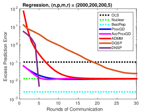
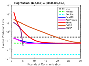
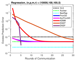
5 Experiments

We first illustrate performance of different procedures on simulated data. We generate data according to

$$y_{ji}\mid\mathbf{x}_{ji}\sim\mathcal{N}(\mathbf{w}_{j}^{T}\mathbf{x}_{ji},1)$$

for regression problems and

$$y_{ji}\mid\mathbf{x}_{ji}\sim{\rm Bernoulli}\left(\left(1+\exp(-\mathbf{w}_{j}^{T}\mathbf{x}_{ji})\right)^{-1}\right)$$

for classification problems. We generate the low-rank $W^{*}$ as follows. We first generate two matrices $A\in\mathbb{R}^{p\times r},B\in\mathbb{R}^{m\times r}$ with entries sampled independently from a standard normal distribution. Then we extract the left and right singular vectors of $AB^{T}$, denoted as $U,V$. Finally, we set $W^{*}=USV^{T}$, where $S$ is a diagonal matrix with exponentially decaying entries: ${\rm diag}(S)=[1,1/1.5,1/(1.5)^{2},\ldots,1/(1.5)^{r}]$. The feature vectors $\mathbf{x}_{ji}$ are sampled from a mean zero multivariate normal with the covariance matrix $\Sigma=(\Sigma_{ab})_{a,b\in[p]}$, $\Sigma_{ab}=2^{-|a-b|}$. The regularization parameters for all approaches were optimized to give the best prediction performance over a held-out validation dataset. For ProxGD and AccProxGD, we initialized the solution from Local. Our simulation results are averaged over 10 independent runs.

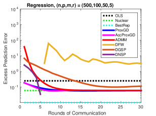
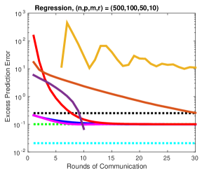
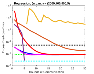
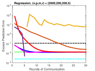
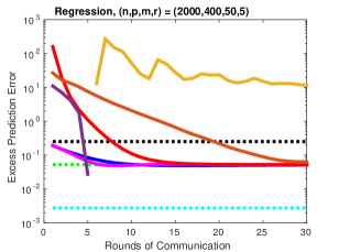
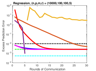
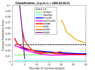
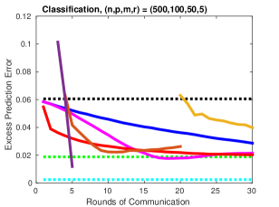
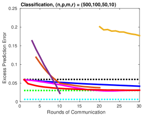
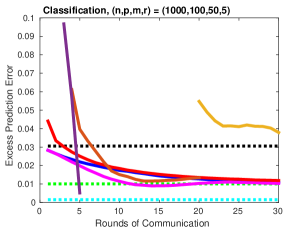
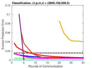
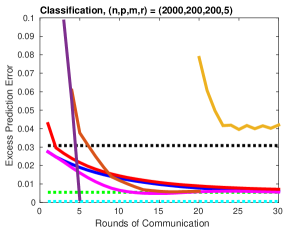
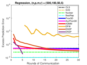
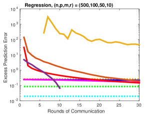
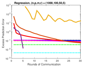
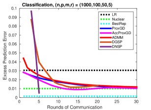
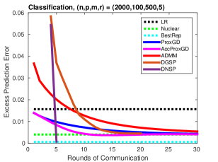
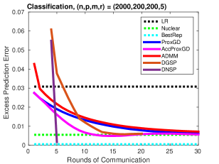
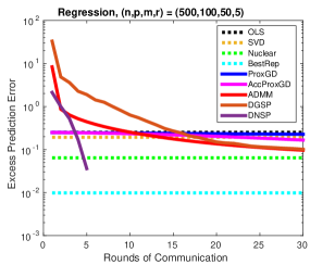
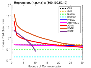
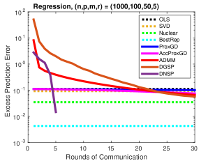
We investigate how the performance of various procedures changes as a function of problem parameters $(n,p,m,r)$. We compare the following procedures: i) Local, where each machine solves an empirical risk minimization problem (ordinary least squares or logistic regression) . ii) Nuclear-norm regularization: which is a popular Centralize approach: all machines send their data to the master, the master solves a nuclear-norm regularized loss minimization problem. iii) Learning with the best representation (BestRep): which assumes the true projection matrix $U$ is known, and just fit ordinal least squares or logistic regression model in the projected low-dimensional subspace . Note that this is not a practical approach since in practice we do not know the best low-dimensional representations of the data. iv) Convex optimization approach which runs distributed optimization algorithms over the nuclear norm-regularized objective: here we implemented and compared the following algorithms: distributed proximal gradient (ProxGD); distributed accelerated proximal gradient, (AccProxGD); distributed alternating direction method of multipliers (ADMM); distributed Frank-Wolfe (DFW) . v) The proposed DGSP and DNSP approaches. The simulation results for regression and classification problems are shown in Figure 1 and 2, respectively. We plot how the excess prediction error decreases as the number of rounds of communications increases (Local, Centralize and BestRep are one shot approaches thus the lines are horizontal). From the plots, we have the following observations:

• Nuclear norm regularization boosts the prediction performance over plain single task learning significantly, which shows clear advantage of leveraging the shared representation in multi-task learning.

• ADMM and AccProxGD perform reasonably well , especially ADMM. One reason for the effectiveness of ADMM is that for the problem of nuclear norm regularized multi-task learning considered here, the ADMM update solves regularized ERM problems at every iteration. ADMM and AccProxGD clearly outperform ProxGD.

• ProxGD and DGSP perform similarly. DGSP usually becomes worse as the iterations increases , while ProxGD converges to a global optimum of the nuclear norm regularized objective.

• DNSP is the most communication-efficient method, and usually converges to a solution that is slightly better compared to the optimum of the nuclear regularization. This shows that second-order information helps a lot in reducing the communication cost.

• The DFW performs the worst in most cases, even though DFW shares some similarity with DGSP in learning the subspace. The empirical results suggest the re-fitting step in DGSP is very important.

One-shot SVD truncation

A natural question to ask is whether there exists a one-shot communication method for the shared representation problem considered here, that still matches the performance of centralized methods. One reasonable solution is to consider the following SVD truncation approach, which is based on the following derivation: consider the following well specified linear regression model:

$$\mathbf{y}_{ji}=\langle{\mathbf{x}_{ji}},{\mathbf{w}_{j}^{*}}\rangle+\epsilon_{ji},$$

where $\epsilon_{ji}$ is drawn from mean-zero Gaussian noise. It is easy to verify the following equation for OLS estimation:

$$\widehat{\mathbf{w}}_{{\rm local}(j)}=\mathbf{w}^{*}_{j}+\left(\sum_{i}\mathbf{x}_{ji}\mathbf{x}_{ji}^{T}\right)^{-1}\left(\sum_{i}\epsilon_{ji}\mathbf{x}_{ji}\right).$$

Since ${\widehat{W}_{\rm local}}$ is just $W^{*}$ plus some mean-zero Gaussian noise, it is natural to consider the following low-rank matrix denoising estimator:

$$\min_{W}||\widehat{W}_{\rm local}-W||_{F}^{2}\quad\text{\rm s.t.}\quad{\rm rank}(W)=r.$$

where the solution is a simple SVD truncation, and can be implemented in a one-shot way: each worker send its Local solution to the master, which then performs an SVD truncation step to maintain the top-$r$ components

$$\widehat{W}_{\rm svd}=U_{r}S_{r}V_{r}^{T},\quad{\rm where}\quad USV^{T}=\texttt{SVD}({\widehat{W}_{\rm local}}),$$

and send the resulting estimation back to each worker, where $U_{r},S_{r},V_{r}$ are top-$r$ components of $U,S,V$. Though this approach might work well for some simple scenarios, but will generally fail when the features are highly correlated: although the Local solution $\widehat{W}_{\rm local}$ can output normal estimation of $W^{*}$, the estimation noise $\left(\sum_{i}\mathbf{x}_{ji}\mathbf{x}_{ji}^{T}\right)^{-1}\left(\sum_{i}\epsilon_{ji}\mathbf{x}_{ji}\right)$ might be highly correlated (depend on the correlation between features), which makes the SVD truncation estimation not reliable. To illustrate this, consider a more complex simulation which follows the same setup as above setting, except that now the feature vectors $\mathbf{x}_{ji}$ are sampled from a higher correlation matrix $\Sigma=(\Sigma_{ab})_{a,b\in[p]}$, $\Sigma_{ab}=2^{-0.1|a-b|}$. The regression simulation results are shown in Figure 3, where we see that the one-shot SVD truncation approach does not significantly outperforms Local, sometimes even slightly worse.

Besides simulation, we also conducted extensive experiments on real world datasets, which are presented in Appendix H due to space limitation.

6 Conclusion

We studied the problem of distributed representation learning for multiple tasks, discussed the implementation and guarantees for distributed convex optimization methods, and presented two novel algorithms to learn low-dimensional projection in a greedy way, which can be communication more efficient than distributed convex optimization approaches. All approaches are extensively evaluated on simulation and real world datasets.

Appendix

Appendix A Distributed Alternating Direction Methods of Multipliers

1 for $t=1,2,\ldots$ do

2       Workers:

3       for $j=1,2,\ldots,m$ do

4             Each worker solves the regularized ERM problem as (A.1) to get $\mathbf{w}_{j}^{(t+1)}$, and send it to the master;

5             Wait;

6             Receive $\mathbf{z}_{j}^{(t+1)},\mathbf{q}_{j}^{(t+1)}$ from master.

7       end for

8      Master:

9       if Receive $\mathbf{w}_{j}^{(t+1)}$ from all workers then

10             Concatenate the current solutions $\mathbf{w}_{j}^{(t+1)}$, and update $Z^{(t+1)}$ as (A.2);

11             Update $Q^{(t+1)}$ as (A.3);

12             Send $\mathbf{z}_{j}^{(t+1)},\mathbf{q}_{j}^{(t+1)}$ to the corresponding worker.

13       end if

14      

15 end for

Algorithm 2 ADMM: Distributed ADMM for Multi-Task Learning.

The Alternating Direction Methods of Multipliers (ADMM) is also a popular method for distributed optimization [11] and can be used to solve the distributed low-rank multi-task learning problem. We first write the objective (2.3) as

$$\arg\min_{W,Z}~{} \mathcal{L}_{n}(W)+\lambda||Z||_{*},\quad{\rm subject\ to}\quad W=Z.$$

By introducing the Lagrangian and augmented terms, we get the following unconstrained problem:

$$\widetilde{\mathcal{L}}(W,Z,Q)= \mathcal{L}_{n}(W)+\lambda||Z||_{*}+\langle{W-Z},{Q}\rangle$$

$$+\frac{\rho}{2}||W-Z||_{F}^{2},$$

where $\rho$ is a parameter controlling the augmentation level. Note that except for $Z$, the augmented Lagrangian objective are decomposable across tasks. To implement the distributed ADMM algorithm, we let the workers maintain the data and $W$, while the master maintains $Z$ and $Q$. At round $t$, each machine separately solves

$$\mathbf{w}_{j}^{(t+1)}=\arg\min_{\mathbf{w}} \mathcal{L}_{nj}(\mathbf{w}_{j})+\langle{\mathbf{w}_{j}^{(t+1)}-\mathbf{z}_{j}^{(t)}},{\mathbf{q}_{j}^{(t)}}\rangle$$

$$+\frac{\rho}{2}||\mathbf{w}_{j}^{(t+1)}-\mathbf{z}_{j}^{(t)}||_{2},$$ (A.1)

which is minimizing the local loss plus a regularization term. Next, each worker sends their solution to the master, which performs the following updates for $Z$ and $Q$

$$Z^{(t+1)}= \arg\min_{Z}~{}\langle{W^{(t+1)}-Z},{Q^{t}}\rangle+\lambda||Z||_{*}$$

$$+\frac{\rho}{2}||W^{(t+1)}-Z||_{F}^{2},$$ (A.2)

$$Q^{(t+1)}= Q^{(t)}+\rho(W^{(t+1)}-Z^{(t+1)}),$$ (A.3)

which have closed-form solutions.

The algorithm ADMM is summarized in Algorithm 2. Note that compared to methods discussed before, ADMM needs to communicate three $p$-dimensional vectors between each worker and the master at each round, while the proximal gradient approaches only communicate two $p$-dimensional vectors per round. Based on convergence results of ADMM [17], $\mathcal{O}\left(\frac{mA^{2}}{\varepsilon}\right)$ rounds of communication are needed to obtain $\varepsilon$-generalization error.

Appendix B Distributed Frank-Wolfe Method

1 for $t=0,2,\ldots$ do

2       Workers:

3       for $j=1,2,\ldots,m$ do

4             Each worker compute the its gradient direction $\nabla\mathcal{L}_{nj}(\mathbf{w}_{j}^{(t)})$, and send it to the master;

5            

6       end for

7      if Receive $\mathbf{v}_{j}\mathbf{u}$ from the master then

8             Set $\gamma=\frac{2}{t+2}$;

9             Update $\mathbf{w}^{(t+1)}_{j}$ as (B.1).

10       end if

11      Master:

12       if Receive $\nabla\mathcal{L}_{nj}(\mathbf{w}_{j}^{(t)})$ from all workers then

13             Concatenate the gradient vectors, and compute the largest singular vectors: $(\mathbf{u},\mathbf{v})=\textsf{SV}(\nabla\mathcal{L}_{n}(W^{(t)}))$;

14             Send $\mathbf{v}_{j}\mathbf{u}$ to $j$-th worker.

15       end if

16      

17 end for

Algorithm 3 DFW: Distributed Frank-Wolfe for Multi-Task Learning.

Another approach we consider is the distributed Frank-Wolfe method [16, 19, 9]. This methods does not require performing SVD, which might bring additional computational advantages. Instead of directly minimizing the nuclear norm regularized objective, the Frank-Wolfe algorithm considers the equivalent constrained minimization problem

$$\min_{W}\mathcal{L}_{n}(W)\quad{\rm subject\ to}\quad||W||_{*}\leq R.$$

At each step, Frank-Wolfe algorithm considers the following direction to update

$$Z^{(t)}=\arg\min_{||Z||_{*}\leq R}\langle{\nabla\mathcal{L}_{n}(W^{(t)})},{Z}\rangle=-R\cdot\mathbf{u}\mathbf{v}^{T},$$

where $(\mathbf{u},\mathbf{v})=\textsf{SV}(\nabla\mathcal{L}_{n}(W^{(t)}))$ is the leading singular vectors of $\nabla\mathcal{L}_{n}(W^{(t)})$. The next iterate is obtained as

$$W^{(t+1)}=(1-\gamma)W^{(t)}+\gamma Z^{(t)},$$

where $\gamma$ is a step size parameter. To implement this algorithm in a distributed way, the master first collects the gradient matrix $\nabla\mathcal{L}_{n}(W^{(t)})$ and computes $\mathbf{u}$ and $\mathbf{v}$. The vector $\mathbf{v}_{j}\mathbf{u}$ is sent to $j$-th machine, which performs the following update:

$$\mathbf{w}_{j}^{(t+1)}=(1-\gamma)\mathbf{w}_{j}^{(t)}-\gamma R\mathbf{v}_{j}\mathbf{u}.$$ (B.1)

The algorithm is summarized in Algorithm 3. Similar to the distributed (accelerated) proximal gradient descent, the distributed Frank-Wolfe only requires communication of two $p$-dimensional vectors per round. Though computationally cheaper compared to other methods considered in this section, the distributed Frank-Wolfe algorithm enjoys similar convergence guarantees to the distributed proximal gradient descent [19], that is, after $\mathcal{O}\left(\frac{mHA^{2}}{\varepsilon}\right)$ iterations, the solution will be $\varepsilon$ suboptimal.

Appendix C Pseudocode of the algorithms

1 for $t=1,2,\ldots$ do

2       Workers:

3       for $j=1,2,\ldots,m$ do

4             Each worker compute the its gradient direction $\nabla\mathcal{L}_{nj}(\mathbf{w}_{j}^{(t)})=\frac{1}{mn}\sum_{i=1}^{n}\ell^{\prime}(\langle{\mathbf{w}^{(t)}_{j}},{\mathbf{x}_{ji}}\rangle,y_{ji})\mathbf{x}_{ji}$, and send it to the master;

5             Wait;

6             Receive $\mathbf{w}_{j}^{(t+1)}$ from master.

7       end for

8      Master:

9       if Receive $\nabla\mathcal{L}_{nj}(\mathbf{w}_{j}^{(t)})$ from all workers then

10             Concatenate the gradient vectors, and update $W^{(t+1)}$ as (3.3);

11             Send $\mathbf{w}_{j}^{(t+1)}$ to all workers.

12       end if

13      

14 end for

Algorithm 4 ProxGD: Distributed Proximal Gradient.

1 for $t=1,2,\ldots$ do

2       Workers:

3       for $j=1,2,\ldots,m$ do

4             Each worker compute the its gradient direction $\nabla\mathcal{L}_{n}(\mathbf{z}_{j}^{(t)})=\frac{1}{mn}\sum_{i=1}^{n}\ell^{\prime}(\langle{\mathbf{z}^{(t)}_{j}},{\mathbf{x}_{ji}}\rangle,y_{ji})\mathbf{x}_{ji}$, and send it to the master;

5             Wait;

6             Receive $\mathbf{z}_{j}^{(t+1)}$ from master.

7       end for

8      Master:

9       if Receive $\nabla\mathcal{L}_{n}(\mathbf{z}_{j}^{(t)})$ from all workers then

10             Concatenate the gradient vectors, and update $W^{(t+1)}$ as (3.4);

11             Update $Z^{(t+1)}$ as (3.5);

12             Send $\mathbf{z}_{j}^{(t+1)}$ to all workers.

13       end if

14      

15 end for

Algorithm 5 AccProxGD: Accelerated Distributed Proximal Gradient for Multi-Task Learning.

1 for $t=1,2,\ldots$ do

2       Workers:

3       for $j=1,2,\ldots,m$ do

4             Each worker computes the Newton direction $\Delta\mathcal{L}_{nj}(\mathbf{w}_{t}^{(t)})=\left(\nabla^{2}\mathcal{L}_{nj}(\mathbf{w}_{t}^{(t)})\right)^{-1}\nabla\mathcal{L}_{nj}(\mathbf{w}_{t}^{(t)})$ and sends it to the master.

5       end for

6      if Receive $\mathbf{u}$ from the master then

7             Perform Gram-Schmidt orthogonalization:

8             $\mathbf{u}\leftarrow\mathbf{u}-\sum_{k=1}^{t-1}\langle{U_{k}},{\mathbf{u}}\rangle$;

9             Normalize $\mathbf{u}=\mathbf{u}/||\mathbf{u}||_{2}$;

10             Update the projection matrix $U=[U~{}\mathbf{u}]$;

11             Solve the projected ERM problem:

12             $\mathbf{v}_{j}=\arg\min_{\mathbf{v}_{j}}\frac{1}{n}\sum_{i=1}^{n}\ell(\langle{\mathbf{v}_{j}},{U^{T}X_{ji}}\rangle,y_{ji})$;

13             Update $\mathbf{w}^{(t+1)}_{j}=U\mathbf{v}_{j}$.

14       end if

15      Master:

16       if Receive $\Delta\mathcal{L}_{nj}(\mathbf{w}_{t}^{(t)})$ from all workers then

17             Concatenate the Newton vectors, and compute the largest singular vectors: $(\mathbf{u},\mathbf{v})=\textsf{SV}(\Delta\mathcal{L}_{n}(W^{(t)}))$;

18             Send $\mathbf{u}$ to all workers.

19       end if

20      

21 end for

Algorithm 6 DNSP: Distributed Newton Subspace Pursuit.

Appendix D Proof of Proposition 4.1

Proof.

It is sufficient to prove that at every iteration, the current projection matrix $U$ and the subspace to be added $\mathbf{u}$ are orthogonal to each other. Note that by the optimality condition:

$$\nabla_{V}\left(\mathcal{L}_{n}(UV^{T})\right)=U^{T}\nabla\mathcal{L}_{n}(W^{(t)})=0.$$

Since $\mathbf{u}$ is the leading left singular vector of $\nabla\mathcal{L}_{n}(W^{(t)})$, we have $U^{T}\mathbf{u}=0$. Each column of $U$ has unit length, since it is a left singular vector of some matrix. ∎

Appendix E Proof of Proposition 4.2

Proof.

It is sufficient to prove that the largest eigenvalue of $\nabla^{2}\mathcal{L}_{n}(W)$ does not exceed $H$. Since $\nabla^{2}\mathcal{L}_{n}(W)$ is a block diagonal matrix, it is sufficient to show that for every block $j\in[m]$, the largest eigenvalue of the block $\nabla^{2}\mathcal{L}_{nj}(\mathbf{w}_{j})$ is not larger than $H$.

This is true by the $H$-smoothness of $\ell(\cdot)$ and the fact that the data points have bounded length:

$$||\nabla^{2}\mathcal{L}_{nj}(\mathbf{w}_{j})||_{2}\leq H\cdot\max_{i,j}||\mathbf{x}_{ji}||_{2}\leq H.$$

∎

Appendix F Proof of Theorem 4.3

Proof.

By the smoothness of $\mathcal{L}_{n}$, we know

$$\mathcal{L}_{n}(W^{(t+1)})\leq \min_{b}\mathcal{L}_{n}(W^{(t)}+b\mathbf{u}\mathbf{v}^{T})$$

$$\leq \mathcal{L}_{n}(W^{(t)})+b\langle{\mathbf{u}\mathbf{v}^{T}},{\nabla\mathcal{L}_{n}(W^{(t)})}\rangle+\frac{Hb^{2}}{2}$$

$$\leq \mathcal{L}_{n}(W^{(t)})+\frac{b\langle{W^{*}},{\nabla\mathcal{L}_{n}(W^{(t)})}\rangle}{||W^{*}||_{F}}+\frac{Hb^{2}}{2}.$$ (F.1)

Let $W^{(t)}=UV^{T}$. Since $V$ is a minimizer of $\mathcal{L}_{n}(UV^{T})$ with respect to $V$, we have $U^{T}\nabla\mathcal{L}_{n}(W^{(t)})=0$ and therefore $\langle{W^{(t)}},{\nabla\mathcal{L}_{n}(W^{(t)})}\rangle={\rm trace}(VU^{T}\nabla\mathcal{L}_{n}(W^{(t)}))=0$. From convexity of $\mathcal{L}_{n}(\cdot)$, we have

$$\langle{W^{*}},{\nabla\mathcal{L}_{n}(W^{(t)})}\rangle= \langle{W^{*}-W^{(t)}},{\nabla\mathcal{L}_{n}(W^{(t)})}\rangle$$

$$\leq \mathcal{L}_{n}(W^{*})-\mathcal{L}_{n}(W^{(t)}).$$

Combining with the display above

$$\mathcal{L}_{n}(W^{(t)})-\mathcal{L}_{n}(W^{(t+1)})\geq \frac{b(\mathcal{L}_{n}(W^{(t)})-\mathcal{L}_{n}(W^{*}))}{||W^{*}||_{F}}$$

$$-\frac{Hb^{2}}{2}.$$

By choosing

$$b=\frac{\mathcal{L}_{n}(W^{(t)})-\mathcal{L}_{n}(W^{*})}{H||W^{*}||_{F}}$$

we have

$$\mathcal{L}_{n}(W^{(t)})-\mathcal{L}_{n}(W^{(t+1)})\geq \frac{\left(\mathcal{L}_{n}(W^{(t)})-\mathcal{L}_{n}(W^{*})\right)^{2}}{2H||W^{*}||_{F}^{2}}$$

$$\geq \frac{\left(\mathcal{L}_{n}(W^{(t)})-\mathcal{L}_{n}(W^{*})\right)^{2}}{2mHA^{2}}.$$

Using Lemma G.1 in Appendix we know that after

$$t\geq\left\lceil\frac{2mHA^{2}}{\varepsilon}\right\rceil$$

iterations, we have $\mathcal{L}_{n}(W^{(t)})\leq\mathcal{L}_{n}(W^{*})+\varepsilon$. ∎

Appendix G An auxiliary lemma

Lemma G.1.

(Lemma B.2 of [34]) Let $x>0$ and let $\varepsilon_{0},\varepsilon_{1},...$ be a sequence such that $\varepsilon\leq\varepsilon_{t}-r\varepsilon_{t}^{2}$ for all $t$. Let $\varepsilon$ be a positive scalar and $t$ be a positive integer such that $t\geq\lceil\frac{1}{x\varepsilon}\rceil$. Then $\varepsilon_{t}\leq\varepsilon$.

Appendix H Evaluation on Real World Datasets

Figure 4: Prediction Error on real data.

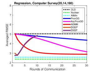
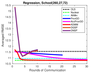
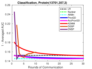
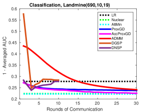
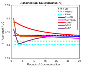
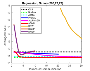
We also evaluate discussed algorithms on several real world data sets, with $20\%$ of the whole dataset as training set, $20\%$ as held-out validation, then report the testing performance on the remaining $60\%$. For the real data, we have observed that adding $\ell_{2}$ regularization usually helps improving the generalization performance. For the Local procedure we added an $\ell_{2}$ regularization term (leads to ridge regression or $\ell_{2}$ regularized logistic regression). For DGSP and DNSP, we also add an $\ell_{2}$ regularization in finding the subspaces and refitting . We have worked on the following multi-task learning datasets:

School. The dataset consists of examination scores of students from London’s secondary schools during the years 1985, 1986, 1987. There are 27 school-specific and student-specific features to describe each student. The instances are divided by different schools, and the task is to predict the students’ performance. We only considered schools with at least $100$ records, which results in 72 tasks in total. The maximum number of records for each individual school is 260.

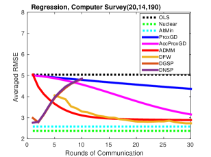
Computer Survey. The data is taken from a conjoint analysis experiment [27] which surveyed 180 persons about the probability of purchasing 20 kinds of personal computers. There are 14 variables for each computer, the response is an integer rating with scale $0-10$.

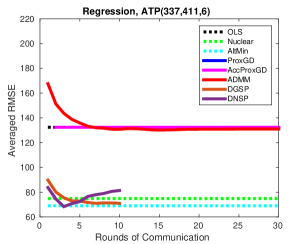
ATP. The task here is to predict the airline ticket price [38]. We are interested in the minimum prices next day for some specific observation date and departure date pairs. Each case is described by 411 features, and there are 6 target minimum prices for different airlines to predict. The sample size is 337.

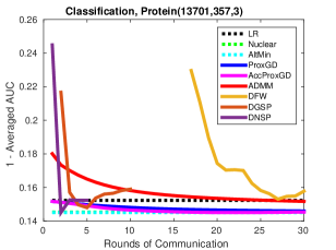
Protein. Given the amino acid sequence, we are interested predicting the protein secondary structure [31]. We tackle the problem by considering the following three binary classification tasks: coil vs helix, helix vs strand, strand vs coil. Each sequence is described by 357 features. There are 24,387 instances in total.

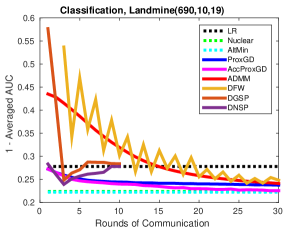
Landmine. The data is collected from 19 landmine detection tasks [44]. Each landmine field is represented by a 9-dimensional vector extracted from radar images, containing moment-based, correlation-based, energy ratio, and spatial variance features. The sample size for each task varies from 445 to 690.

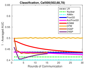
Cal500. This music dataset [40] consists of 502 songs, where for each song 68 features are extracted. Each task is to predict whether a particular musically relevant semantic keyword should be an annotation for the song. We only consider tags with at least 50 times apperance, which results in 78 prediction tasks.

We compared various approaches as in the simulation study, except the BestRep as the best low-dimensional representation is unknown. We also compared with AltMin, which learns low-rank prediction matrix using the alternating minimization [21]. The results are shown in Figure 4. Since the labels for the real world classification datasets are often unbalanced, we report averaged area under the curve (AUC) instead of classification accuracy. We have the following observations:

• The distributed first-order approaches converge much slower than in simulations, especially on ATP and Cal500. We suspect this is because in the simulation study, the generated data are usually well conditioned, which makes faster convergence possible for such methods [1, 18]. On real data, the condition number can be much worse.

• In most case, DNSP is the best in terms of communication-efficiency. DGSP also has reasonable performance with fewer round of communications compared to distributed first-order approaches.

• Among the first-order distributed convex optimization methods, AccProxGD is overall the most communication-efficient, while DFW is the worst, though it might have some advantages in terms of computation. Also, we observed significant zig-zag behavior of the DFW algorithm, as discussed in [24].

Appendix I Full experimental results with Distributed Frank-Wolfe

Figure 5: Excess prediction error for multi-task regression.

Figure 6: Excess prediction error for multi-task classification.

Figure 7: Excess prediction error for multi-task regression, with highly correlated features.

Figure 8: Prediction Error on real data.

References

- Agarwal et al. (2012) A. Agarwal, S. Negahban, and M. J. Wainwright. Fast global convergence of gradient methods for high-dimensional statistical recovery. Ann. Stat., 40(5):2452–2482, 2012.
- Amit et al. (2007) Y. Amit, M. Fink, N. Srebro, and S. Ullman. Uncovering shared structures in multiclass classification. In ICML, pages 17–24. ACM, 2007.
- Ando and Zhang (2005) R. K. Ando and T. Zhang. A framework for learning predictive structures from multiple tasks and unlabeled data. J. Mach. Learn. Res., 6:1817–1853, 2005.
- Argyriou et al. (2008) A. Argyriou, T. Evgeniou, and M. Pontil. Convex multi-task feature learning. Mach. Learn., 73(3):243–272, 2008.
- Bach et al. (2011) F. Bach, R. Jenatton, J. Mairal, and G. Obozinski. Optimization with sparsity-inducing penalties. Found. Trends Mach. Learn., 4(1):1–106, 2011.
- Balcan et al. (2012) M.-F. Balcan, A. Blum, S. Fine, and Y. Mansour. Distributed learning, communication complexity and privacy. In JMLR W&CP 23: COLT 2012, volume 23, pages 26.1–26.22, 2012.
- Bartlett and Mendelson (2002) P. L. Bartlett and S. Mendelson. Rademacher and gaussian complexities: Risk bounds and structural results. J. Mach. Learn. Res., 3:463–482, 2002.
- Bekkerman et al. (2011) R. Bekkerman, M. Bilenko, and J. Langford. Scaling up machine learning: Parallel and distributed approaches. Cambridge University Press, 2011.
- Bellet et al. (2015) A. Bellet, Y. Liang, A. B. Garakani, M.-F. Balcan, and F. Sha. A distributed frank-wolfe algorithm for communication-efficient sparse learning. In SDM, pages 478–486. 2015.
- Bousquet and Bottou (2008) O. Bousquet and L. Bottou. The tradeoffs of large scale learning. In NIPS, pages 161–168, 2008.
- Boyd et al. (2011) S. P. Boyd, N. Parikh, E. Chu, B. Peleato, and J. Eckstein. Distributed optimization and statistical learning via the alternating direction method of multipliers. Found. Trends Mach. Learn., 3(1):1–122, 2011.
- Cai et al. (2010) J.-F. Cai, E. J. Candès, and Z. Shen. A singular value thresholding algorithm for matrix completion. SIAM Journal on Optimization, 20(4):1956–1982, 2010.
- Caruana (1997) R. Caruana. Multitask learning. Mach. Learn., 28(1):41–75, 1997.
- Chapelle et al. (2010) O. Chapelle, P. Shivaswamy, S. Vadrevu, K. Weinberger, Y. Zhang, and B. Tseng. Multi-task learning for boosting with application to web search ranking. In KDD, pages 1189–1198. ACM, 2010.
- Collobert et al. (2011) R. Collobert, J. Weston, L. Bottou, M. Karlen, K. Kavukcuoglu, and P. Kuksa. Natural language processing (almost) from scratch. J. Mach. Learn. Res., 12:2493–2537, 2011.
- Frank and Wolfe (1956) M. Frank and P. Wolfe. An algorithm for quadratic programming. Naval research logistics quarterly, 3(1-2):95–110, 1956.
- He and Yuan (2012) B. He and X. Yuan. On the convergence rate of the douglas-rachford alternating direction method. SIAM Journal on Numerical Analysis, 50(2):700–709, 2012.
- Hong and Luo (2012) M. Hong and Z.-Q. Luo. On the linear convergence of the alternating direction method of multipliers. ArXiv e-prints, arXiv:1208.3922, 2012.
- Jaggi (2013) M. Jaggi. Revisiting frank-wolfe: Projection-free sparse convex optimization. In ICML, pages 427–435, 2013.
- Jaggi et al. (2014) M. Jaggi, V. Smith, M. Takác, J. Terhorst, S. Krishnan, T. Hofmann, and M. I. Jordan. Communication-efficient distributed dual coordinate ascent. In NIPS, pages 3068–3076, 2014.
- Jain et al. (2013) P. Jain, P. Netrapalli, and S. Sanghavi. Low-rank matrix completion using alternating minimization. In STOC, pages 665–674. ACM, 2013.
- Ji and Ye (2009) S. Ji and J. Ye. An accelerated gradient method for trace norm minimization. In ICML, pages 457–464. ACM, 2009.
- Kim and Xing (2010) S. Kim and E. P. Xing. Tree-guided group lasso for multi-task regression with structured sparsity. In ICML, pages 543–550, 2010.
- Lacoste-Julien and Jaggi (2015) S. Lacoste-Julien and M. Jaggi. On the global linear convergence of frank-wolfe optimization variants. In NIPS, pages 496–504, 2015.
- Lapin et al. (2014) M. Lapin, B. Schiele, and M. Hein. Scalable multitask representation learning for scene classification. In CVPR, pages 1434–1441, 2014.
- Lee et al. (2015) J. D. Lee, Y. Sun, Q. Liu, and J. E. Taylor. Communication-efficient sparse regression: a one-shot approach. ArXiv e-prints, arXiv:1503.04337, 2015.
- Lenk et al. (1996) P. J. Lenk, W. S. DeSarbo, P. E. Green, and M. R. Young. Hierarchical bayes conjoint analysis: Recovery of partworth heterogeneity from reduced experimental designs. Marketing Science, 15(2):173–191, 1996.
- Maurer and Pontil (2013) A. Maurer and M. Pontil. Excess risk bounds for multitask learning with trace norm regularization. pages 55–76, 2013.
- Nesterov (1983) Y. Nesterov. A method of solving a convex programming problem with convergence rate . In Soviet Mathematics Doklady, volume 27, pages 372–376, 1983.
- Ram et al. (2010) S. S. Ram, A. Nedić, and V. V. Veeravalli. Distributed stochastic subgradient projection algorithms for convex optimization. Journal of optimization theory and applications, 147(3):516–545, 2010.
- Sander and Schneider (1991) C. Sander and R. Schneider. Database of homology-derived protein structures and the structural meaning of sequence alignment. Proteins: Structure, Function, and Bioinformatics, pages 56–68, 1991.
- Seltzer and Droppo (2013) M. L. Seltzer and J. Droppo. Multi-task learning in deep neural networks for improved phoneme recognition. In ICASSP, pages 6965–6969. IEEE, 2013.
- Shalev-Shwartz and Ben-David (2014) S. Shalev-Shwartz and S. Ben-David. Understanding machine learning: From theory to algorithms. Cambridge University Press, 2014.
- Shalev-Shwartz et al. (2010) S. Shalev-Shwartz, N. Srebro, and T. Zhang. Trading accuracy for sparsity in optimization problems with sparsity constraints. SIAM Journal on Optimization, 20(6):2807–2832, 2010.
- Shalev-Shwartz et al. (2011) S. Shalev-Shwartz, A. Gonen, and O. Shamir. Large-scale convex minimization with a low-rank constraint. In ICML, 2011.
- Shamir and Srebro (2014) O. Shamir and N. Srebro. Distributed stochastic optimization and learning. In Allerton, pages 850–857. IEEE, 2014.
- Shamir et al. (2014) O. Shamir, N. Srebro, and T. Zhang. Communication efficient distributed optimization using an approximate newton-type method. In ICML, pages 1000–1008, 2014.
- Spyromitros-Xioufis et al. (2012) E. Spyromitros-Xioufis, G. Tsoumakas, W. Groves, and I. Vlahavas. Multi-target regression via input space expansion: Treating targets as inputs. ArXiv e-prints, arXiv:1211.6581, 2012.
- Tropp (2004) J. A. Tropp. Greed is good: Algorithmic results for sparse approximation. IEEEit, 50(10):2231–2242, 2004.
- Turnbull et al. (2008) D. Turnbull, L. Barrington, D. Torres, and G. Lanckriet. Semantic annotation and retrieval of music and sound effects. IEEE Transactions on Acoustics, Speech and Signal Processing, 16(2):467–476, 2008.
- Wang et al. (2015a) J. Wang, M. Kolar, and N. Srebro. Distributed multitask learning. ArXiv e-prints, arXiv:1510.00633, 2015a.
- Wang et al. (2015b) Z. Wang, M.-J. Lai, Z. Lu, W. Fan, H. Davulcu, and J. Ye. Orthogonal rank-one matrix pursuit for low rank matrix completion. SIAM Journal on Scientific Computing, 37(1):A488–A514, 2015b.
- Weinberger et al. (2009) K. Weinberger, A. Dasgupta, J. Langford, A. Smola, and J. Attenberg. Feature hashing for large scale multitask learning. In ICML, pages 1113–1120. ACM, 2009.
- Xue et al. (2007) Y. Xue, X. Liao, L. Carin, and B. Krishnapuram. Multi-task learning for classification with dirichlet process priors. J. Mach. Learn. Res., 8:35–63, 2007.
- Yuan et al. (2007) M. Yuan, A. Ekici, Z. Lu, and R. Monteiro. Dimension reduction and coefficient estimation in multivariate linear regression. J. R. Stat. Soc. B, 69(3):329–346, 2007.
- Zhang and Xiao (2015) Y. Zhang and L. Xiao. Communication-efficient distributed optimization of self-concordant empirical loss. ArXiv e-prints, arXiv:1501.00263, 2015.
- Zhang et al. (2012) Y. Zhang, M. J. Wainwright, and J. C. Duchi. Communication-efficient algorithms for statistical optimization. In NIPS, pages 1502–1510, 2012.
- Zhang et al. (2013) Y. Zhang, J. C. Duchi, M. I. Jordan, and M. J. Wainwright. Information-theoretic lower bounds for distributed statistical estimation with communication constraints. In NIPS, pages 2328–2336, 2013.
- Zhou et al. (2013) J. Zhou, J. Liu, V. A. Narayan, and J. Ye. Modeling disease progression via multi-task learning. NeuroImage, 78:233 – 248, 2013.