Functional renormalization group analysis of the soft mode at the QCD critical point

Abstract

We make an intensive investigation of the soft mode at the quantum chromodynamics (QCD) critical point on the basis of the functional renormalization group (FRG) method in the local potential approximation. We calculate the spectral functions $\rho_{\sigma,\pi}(\omega,\,p)$ in the scalar ($\sigma$) and pseudoscalar ($\pi$) channels beyond the random phase approximation in the quark–meson model. At finite baryon chemical potential $\mu$ with a finite quark mass, the baryon-number fluctuation is coupled to the scalar channel and the spectral function in the $\sigma$ channel has a support not only in the time-like ($\omega\,>\,p$) but also in the space-like ($\omega\,<\,p$) regions, which correspond to the mesonic and the particle–hole phonon excitations, respectively. We find that the energy of the peak position of the latter becomes vanishingly small with the height being enhanced as the system approaches the QCD critical point, which is a manifestation of the fact that the phonon mode is the soft mode associated with the second-order transition at the QCD critical point, as has been suggested by some authors. Moreover, our extensive calculation of the spectral function in the $(\omega,p)$ plane enables us to see that the mesonic and phonon modes have the respective definite dispersion relations $\omega_{\sigma.{\rm ph}}(p)$, and it turns out that $\omega_{\sigma}(p)$ crosses the light-cone line into the space-like region, and then eventually merges into the phonon mode as the system approaches the critical point more closely. This implies that the sigma-mesonic mode also becomes soft at the critical point. We also provide numerical stability conditions that are necessary for obtaining the accurate effective potential from the flow equation.

B32, D30, D31

1 Introduction

The phase diagram of quantum chromodynamics (QCD) is expected to have a rich structure and its clarification is one of the main topics in high-energy and nuclear physics Fukushima:2010bq . One of the remarkable features in the expected phase structure is the existence of the first-order phase boundary between the hadronic phase and the quark–gluon plasma (QGP) phase at large baryon chemical potential $\mu$. In particular, the end point of the first-order phase boundary is known as the QCD critical point, where the phase transition becomes second order. Although lattice QCD, which is a powerful nonperturbative first-principle method for QCD, has a limited predictive power in the case of large $\mu$ because of the sign problem Muroya:2003 ; deForcrand:2009 ; Aarts:2015 , other QCD-motivated approaches, such as chiral effective models implementing relevant symmetries and functional methods with inputs from lattice QCD, support the existence of the QCD critical point Asakawa:1989bq ; Hatsuda:1994pi ; Halasz:1998 ; Scavenius:2001 ; Buballa:2003qv ; Fukushima:2003fw ; Ratti:2005jh ; Schaefer:2005 ; Schaefer:2007pw ; Herbst:2013 ; Fischer:2014 ; Stiele:2016cfs .

While the location of the QCD critical point in these calculations strongly depends on details of the models and employed approximations Stephanov:2004PTEP ; Sasaki:2007 ; Kashiwa:2008 ; Nakano:2010 , one may expect anomalous fluctuations of experimental observables in relativistic heavy ion collisions if the produced matter passes through critical region where the thermodynamic quantities are strongly influenced by the existence of the critical point Stephanov:1999zu . In particular, the net-baryon number susceptibility and its higher-order ones, approximated by the net-proton ones in measurements Hatta-Stephanov , are expected to be sensitive to the critical behavior of the system Hatta:2002sj ; Sasaki:2007 ; Asakawa:2009prl ; Stephanov:2009prl ; Stephanov:2011prl ; Skokov:2011prc ; Friman:2011epjc ; Morita:2013prob ; Morita:2013prob2 ; Morita:2013prob3 ; Ichihara:2015 . A recent summary of measurements in the beam-energy scan program at the Relativistic Heavy Ion Collider (RHIC) including intriguing behaviors of the net-proton fluctuations can be found in Ref. BES .

Although the mean-field theory seems to give a reasonable picture of the phase structure, a system near a critical point exhibits strong correlations among its constituents. Therefore methods beyond the mean-field theory are desirable for understanding the physics near the critical point. The functional renormalization group (FRG) Wetterich:1992yh ; Wegner:1972ih ; Wilson:1974 ; Polchinski:1983gv is one of the frameworks that enables us to incorporate fluctuation effects beyond the mean-field theory; see also Refs. Berges:2000ew ; Pawlowski:2005xe ; Gies:2006wv . Indeed, it has been pointed out that such fluctuations play an important role in the aforementioned observables Skokov:2010 ; Skokov:2011prc ; Morita:2013prob ; Morita:2013prob2 ; Morita:2013prob3 ; Ichihara:2015 ; Morita:2015 ; Fu-Pawlowski:2015 . The FRG has been applied to a wide range of fields including hot and dense QCD and found to be useful in the description of chiral phase transition in QCD using effective chiral models Jungnickel:1995fp ; Braun:2003ii ; Schaefer:2005 ; Schaefer:2006ds ; Stokic:2010 ; Nakano:2010 ; Aoki:2014 .

For a second-order transition, there exist specific modes that are coupled to the fluctuations of the order parameter and become gapless and long-lived at the critical point. Such a mode is called the soft mode of the phase transition. As for the QCD critical point, the nature of the soft modes changes depending on whether the quarks have a mass or not Fujii:2004jt ; Son:2004iv : In the chiral limit where the quarks are massless, the theory has exact chiral symmetry and an O(4) critical line appears in the $(T,\,\mu)$ plane in the two-flavor case; the critical line terminates at a point (the tricritical point) in the $(T,\,\mu)$ plane and is connected to a first-order phase transition line Pisarski:1984 ; the $\sigma$ and $\pi$ mesonic modes in the time-like region become massless on the critical line, implying that the quartet mesons are the soft modes of the chiral transition in the chiral limit Hatsuda:1985ey ; Hatsuda:1985ey2 ; Hatsuda:1985eb . At finite baryon chemical potential, however, the picture changes because the charge conjugation symmetry is lost. When the chiral symmetry is broken, the mixed correlator $\langle\langle\bar{\psi}\psi\bar{\psi}\gamma^{0}\psi\rangle\rangle$ does not vanish. Then, when the system approaches the tricritical point in the broken phase, the density fluctuation $\langle\langle(\bar{\psi}\gamma^{0}\psi)^{2}\rangle\rangle$ also shows a singular behavior. Furthermore, when the theory does not have chiral symmetry due to the current quark masses from the outset, the natures of the phase transition and the soft mode change drastically. In this case, the tricritical point becomes the critical point where the universality class belongs to that of the $Z_{2}$ critical point and the soft mode is considered to be the particle–hole mode corresponding to the density (and energy) fluctuations. It is noteworthy that not only the chiral susceptibility but also the susceptibilities of hydrodynamical modes such as the density fluctuation or the quark-number susceptibility diverge at the critical point, owing to the scalar–vector coupling caused by the finite quark mass at nonvanishing $\mu$ Kunhiro:1991 . Such a picture is suggested in the time-dependent Ginzburg–Landau theory and random phase approximation (RPA) analysis of the Nambu–Jona-Lasino (NJL) model in Ref. Fujii:2004jt and the Langevin equation in Ref. Son:2004iv .

Then it would be intriguing to apply the FRG for investigating the nature and dynamical properties of the soft mode at the critical point, which is the purpose of the present work. Here it should be mentioned that the role of density fluctuations in the static critical properties of the QCD critical point has been investigated in FRG within a chiral quark–meson model Kamikado:2012cp , where static properties such as the quark–number susceptibility and the curvature (screening) masses in the scalar and vector channels are analyzed. Dynamical properties such as the dispersion relations of excitation modes and those of the soft modes at the QCD critical point have not been touched upon. We note that these quantities can be read off from the spectral function in the relevant channel.

Needless to say, a real-time analysis is needed for the investigation of the spectral functions for excitation modes. Since analytic continuation of the two-point functions from imaginary Matsubara frequencies to real frequencies is necessary to get real-time two-point Green’s functions at finite temperature, it is in general difficult to obtain the spectral functions numerically with high accuracy Jarrell:1996 ; Asakawa:2000tr ; Vidberg:1977 ; Dudal:2013yva . Recently, a useful method for calculating the spectral functions within FRG has been developed, which adopts an unambiguous way of analytic continuation in the imaginary-time formalism and leads to reasonable results of meson spectral functions in the O(4) model in vacuum Kamikado:2013sia . Furthermore, this method has also been successfully applied to the quark–meson model at finite temperature and chemical potential Tripolt:2013jra ; Tripolt:2014wra .

The spectral function in a specific channel with specific quantum numbers may have more than one peak and bump, the number of which can change according to that of the parameters characterizing the system such as temperature and baryon density. A peak or even bump in the spectral function in the channel may be identified with a particle excitation in the channel, and the width of the peak/bump shows the decay rate of the particle in a specific decay channel. This feature enables one not only to explore the appearance but also to analyze the nature of modes in the system using spectral functions in various channels. In particular, the spectral functions around a critical point give information on the soft modes. Actually, the spectral function in the scalar–isoscalar channel, i.e., the sigma channel, has been analyzed in the RPA using the Nambu–Jona-Lasinio (NJL) model in Ref. Fujii:2004jt , where it is shown that the spectral function has a prominent bump in the space-like region corresponding to the phonon mode composed of particle–hole excitations, the peak position of which moves to vanishingly small frequency as the system approaches the critical point, whereas the mesonic sigma mode in the time-like region does not show such a behavior, retaining a finite mass. This result clearly shows that the phonon mode (or hydrodynamical mode in general) is the soft mode of the QCD critical point; see also Refs. Son:2004iv ; Minami:2009hn ; Minami:2009hn2 ; Minami:2009hn3 .

The purpose of the present paper is to investigate the nature of low-energy modes at the QCD critical point beyond the RPA using a two-flavor quark–meson model: We calculate the spectral functions in the $\sigma$ and pion channels with FRG. Our results confirm the softening of the particle–hole mode in the $\sigma$ channel near the QCD critical point, but not in the pion channel. In addition, we find that the low-momentum dispersion relation of the sigma-mesonic mode penetrates into the space-like region and the mode merges into the bump of the particle–hole mode.

This paper is organized as follows. In Sect. 2, we recapitulate the method Tripolt:2013jra ; Tripolt:2014wra and describe how to calculate the spectral functions in the mesonic channels numerically with FRG. The numerical results are shown in Sect. 3. The phase diagram, the critical region, and the precise location of the critical point are presented in Sect. 3.2. In Sect. 3.4 the results of the spectral functions are shown, and the soft mode at the QCD critical point is discussed. Section 4 is devoted to the summary and outlook. In Appendix A, the detailed forms of the FRG flow equations after Matsubara summation are shown. In Appendix B, we derive the conditions for numerically stable calculation of the flow equation as a nonlinear partial differential equation.

2 Method

In this section, we recapitulate the method developed in Refs. Tripolt:2013jra ; Tripolt:2014wra for calculating spectral functions in the quark–meson model with FRG, and present some details of our numerical procedure.

2.1 Procedure to derive spectral functions in meson channels

The FRG is based on the philosophy of the Wilsonian renormalization group and realizes the coarse graining by introducing a regulator function $R_{k}$ , which has the role of suppressing lower-momentum modes than the scale $k$ for the respective field. In this method, the effective average action (EAA) $\Gamma_{k}$ is introduced such that it becomes bare action $S_{\Lambda}$ at a large UV scale $k=\Lambda$ and becomes the effective action at $k\rightarrow 0$ with an appropriate choice of regulators. The flow equation for EAA, the Wetterich equation, can be derived as a functional differential equation Wetterich:1992yh :

$$\partial_{k}\Gamma_{k}=\frac{1}{2}\mathrm{STr}\left[\frac{\partial_{k}R_{k}}{\Gamma^{(2)}_{k}+R_{k}}\right],$$ (1)

where $\Gamma_{k}^{(n)}$ is the $n$th functional derivative of $\Gamma_{k}$ with respect to fields. This equation has a one-loop structure and can be represented diagrammatically (Fig. 1 (a)).

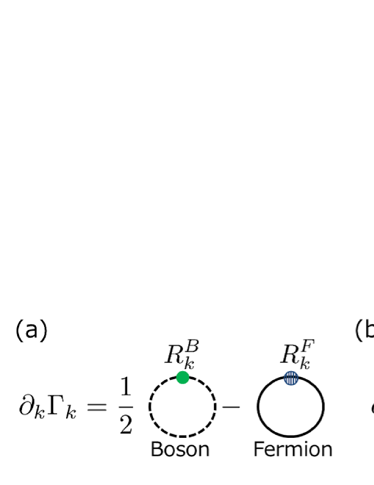
Figure 1: Diagrammatic representations of (a) Eq. (1) and (b) Eq. (5).

In principle, one can get the effective action $\Gamma_{k=0}$ by solving Eq. (1) with the initial condition $\Gamma_{\Lambda}=S_{\Lambda}$.

However, it is prohibitively difficult to solve Eq. (1) in an exact way and some simplifications are introduced for practical use. One of the simplifications is to truncate the form of EAA. Since our purpose is to reveal the behavior of the low-momentum modes around the QCD critical point, we adopt a truncation in which the low-momentum fluctuations are properly taken into account.

We should now specify the low-energy effective model of QCD; we employ the two-flavor quark–meson model as such a model. Then we take the local potential approximation (LPA) for the meson flow part as our truncation. This truncation corresponds to considering only the lowest order of derivative expansion for the meson flow part.

In the imaginary-time formalism, our truncated EAA is as follows Schaefer:2006ds :

$$\Gamma_{k}\left[\overline{\psi},\psi,\phi\right]= \int_{0}^{\frac{1}{T}}d\tau\int d^{3}x\left\{\overline{\psi}\left({\ooalign{\hfil/\hfil\crcr$\partial$}}+g_{s}(\sigma+i\vec{\tau}\cdot\vec{\pi}\gamma_{5})-\mu\gamma_{0}\right)\psi+\frac{1}{2}(\partial_{\mu}\phi)^{2}+U_{k}(\phi^{2})-c\sigma\right\},$$ (4)

where $\phi=(\sigma,\vec{\pi})$. The quark field $\psi$ has the indices of a four-component spinor, color $N_{c}=3$, and flavor $N_{f}=2$. The $c\sigma$ represents the effect of the current quark mass, which explicitly breaks $N_{f}=2$ chiral symmetry. In this truncation, we also neglect the flow of $g_{s}$ and the wave function renormalization. Therefore, only the meson effective potential $U_{k}$ has a $k$ dependence.

Although the truncated EAA itself gives only the simplest information about the momentum dependence of two-point Green’s functions, the nonperturbative effects are to be incorporated through Eq. (1) with the truncated EAA used as the initial condition. More specifically, we first calculate the effective potential $U_{k}(\phi^{2})$ using Eq. (1). Then the chiral condensate $\sigma_{0}$ is obtained as $\sigma$ satisfying the quantum equation of motion (EOM) $\delta\Gamma_{k=0}/\delta\sigma=0$. In our case, this condition corresponds to obtaining $\sigma$ that minimizes $U_{k}(\sigma^{2})-c\sigma$, under the assumptions that the condensate is homogeneous and $\langle\vec{\pi}\rangle=\vec{0}$. Next, we derive the flow equations for two-point Green’s functions. Such flow equations can be derived from the flow equation for $\Gamma^{(2)}_{k}$ by differentiating both sides of Eq. (1):

$$\partial_{k}\Gamma^{(2)}_{k}= \mathrm{STr}\left[\frac{1}{\Gamma^{(2)}_{k}+R_{k}}\Gamma^{(3)}_{k}\frac{1}{\Gamma^{(2)}_{k}+R_{k}}\Gamma^{(3)}_{k}\frac{1}{\Gamma^{(2)}_{k}+R_{k}}\partial_{k}R_{k}\right]-\frac{1}{2}\mathrm{STr}\left[\frac{1}{\Gamma^{(2)}_{k}+R_{k}}\Gamma^{(4)}_{k}\frac{1}{\Gamma^{(2)}_{k}+R_{k}}\partial_{k}R_{k}\right].$$ (5)

The diagrammatic expression of this equation is shown in Fig. 1 (b). If the fields in Eq. (5) are replaced by those satisfying the quantum EOM, Eq. (5) becomes the flow equations for the inverses of the two-point Green’s functions. Then, Eq. (5) can be rewritten as the flow equations for the inverses of the two-point temperature Green’s functions $\Gamma^{(2)}_{k,\sigma}(P)$ and $\Gamma^{(2)}_{k,\pi}(P)$ in the sigma and pion channels, respectively, which are defined as

$$\left.\frac{\delta^{2}\Gamma_{k}}{\delta\sigma(P)\delta\sigma(Q)}\right|_{\overline{\psi}=0,\psi=0,\vec{\pi}=\vec{0},\sigma=\sigma_{0}} =(2\pi)^{4}\delta^{(4)}(P+Q)\Gamma^{(2)}_{k,\sigma}(P),$$ (6)

$$\left.\frac{\delta^{2}\Gamma_{k}}{\delta\pi_{a}(P)\delta\pi_{a}(Q)}\right|_{\overline{\psi}=0,\psi=0,\vec{\pi}=\vec{0},\sigma=\sigma_{0}} =(2\pi)^{4}\delta^{(4)}(P+Q)\Gamma^{(2)}_{k,\pi}(P),$$ (7)

where $\sigma(P)$ and $\pi_{a}(P)$ are the Fourier transforms of $\sigma(x)$ and $\pi_{a}(x)$, respectively, and $P=(i\omega_{n},\vec{p})$ with $\omega_{n}$ being the bosonic Matsubara frequency. The RHS of Eq. (5) contains $\Gamma_{k}^{(2)}$, $\Gamma_{k}^{(3)}$, and $\Gamma_{k}^{(4)}$. In general, the flow equation comprises an infinite hierarchy of differential equations such that the flow equation for $\Gamma_{k}^{(n)}$ contains $\Gamma_{k}^{(n+1)}$ and $\Gamma_{k}^{(n+2)}$. We can simplify the flow equation for the $\Gamma^{(n)}_{k}$ by replacing these derivatives with those derived from the truncated EAA. Under the above procedure, the integration of the flow equation for $\Gamma^{(2)}_{k,\sigma(\pi)}(P)$ leads to the two-point Green’s function in the sigma (pion) channel with the nonperturbative effects incorporated.

A real-time two-point Green’s function at finite temperature is obtained by analytic continuation for the temperature Green’s function to real time, i.e., from imaginary Matsubara frequencies to real frequencies in the case of momentum representation. In our case, such an analytic continuation is successfully carried out at the level of the flow equation after the Matsubara summations in the RHS of Eq. (5), as follows: When one derives a retarded two-point Green’s function via analytic continuation in the frequency $\omega$ plane, the analyticity of the Green’s function in the upper half-plane of $\omega$ must be retained BM1961 . In the present case, the flow equation itself should be analytic in the upper half-plane after the analytic continuation. One can retain the analyticity in the upper half-plane easily by taking into account the following points. First, by choosing $\omega_{n}$-independent regulators, one can avoid possible extra poles in the $\omega$ plane in the flow equation otherwise arising from $\omega_{n}$ dependence of the regulators. The second point is about the analytic continuation of thermal distribution functions $n_{B,F}(E+i\omega_{n})$ obtained for a discrete (multiple of $2\pi T$) frequency $\omega_{n}$, where the subscript $B$, $F$ stands for a boson or fermion, respectively, and $E$ is $\omega_{n}$ independent. Such factors appear in the flow equation after the Matsubara summation. Because of the periodicity of the exponential function, $n_{B,F}(E+i\omega_{n})$ is equal to $n_{B,F}(E)$. However if $n_{B,F}(E+\omega)$ is substituted for $n_{B,F}(E+i\omega_{n})$, such a factor breaks the analyticity of the flow equation in the upper half-plane. Therefore $n_{B,F}(E+i\omega_{n})$ should be replaced by $n_{B,F}(E)$ before the analytic continuation. By taking into account these points, the substitution $\omega+i\epsilon$ for $i\omega_{n}$ with $\epsilon$ being a positive infinitesimal gives the flow equation for the inverse of the retarded Green’s function $\Gamma^{(2),R}_{k,\sigma,\pi}(\omega,\vec{p})$. Finally, the spectral functions in the meson channels are given in terms of the thus-obtained retarded Green’s functions as follows:

$$\rho_{\sigma}(\omega,\vec{p}) =\frac{1}{\pi}\mathrm{Im}\frac{1}{\Gamma^{(2),R}_{k\rightarrow 0,\sigma}(\omega,\vec{p})},$$ (8)

$$\rho_{\pi}(\omega,\vec{p}) =\frac{1}{\pi}\mathrm{Im}\frac{1}{\Gamma^{(2),R}_{k\rightarrow 0,\pi}(\omega,\vec{p})}.$$ (9)

2.2 Flow equations

In the present work, we adopt the 3D Litim’s optimized regulators for bosons and fermions Litim:2001up as $\omega_{n}$-independent regulators:

$$R^{B}_{k}(Q) = (k^{2}-\vec{q}^{2})\theta(k^{2}-\vec{q}^{2}),$$ (10)

$$R^{F}_{k}(Q) = i{\ooalign{\hfil/\hfil\crcr$\vec{q}$}}\left(\sqrt{\frac{k^{2}}{\vec{q}^{2}}}-1\right)\theta(k^{2}-\vec{q}^{2}).$$ (13)

Then the insertion of Eq. (4) into Eq. (1) leads to the following flow equation for $U_{k}$:

$$\partial_{t}U_{k}=\frac{k^{5}}{12\pi^{2}} \left[-2N_{f}N_{c}\left[\frac{1}{E_{\psi}}\tanh\frac{E_{\psi}+\mu}{2T}+\frac{1}{E_{\psi}}\tanh\frac{E_{\psi}-\mu}{2T}\right]+\frac{1}{E_{\sigma}}\coth\frac{E_{\sigma}}{2T}+\frac{3}{E_{\pi}}\coth\frac{E_{\pi}}{2T}\right],$$ (14)

where $t=\ln(k/\Lambda)$, $E_{a}=\sqrt{k^{2}+m^{2}_{a}}\ (a=\psi,\sigma,\pi)$, and

$$m^{2}_{\psi}=g^{2}_{s}\sigma^{2},\ m^{2}_{\sigma}=\partial^{2}_{\sigma}U_{k},\ m^{2}_{\pi}=\partial_{\sigma}U_{k}/\sigma.$$ (15)

According to the procedure presented in the previous subsection, the flow equations for $\Gamma^{(2)}_{k,\sigma}(P)$ and $\Gamma^{(2)}_{k,\pi}(P)$ become:

$$\partial_{k}\Gamma^{(2)}_{k,\sigma}(P)= J_{k,\sigma\sigma}(P)(\Gamma^{(0,3)}_{k,\sigma\sigma\sigma})^{2}-\frac{1}{2}I^{(2)}_{k,\sigma}\Gamma^{(0,4)}_{k,\sigma\sigma\sigma\sigma}+3J_{k,\pi\pi}(P)(\Gamma^{(0,3)}_{k,\sigma\pi\pi})^{2}-\frac{3}{2}I^{(2)}_{k,\pi}\Gamma^{(0,4)}_{k,\sigma\sigma\pi\pi}$$

$$-2N_{c}N_{f}J^{(\sigma)}_{k,\bar{\psi}\psi}(P),$$ (16)

$$\partial_{k}\Gamma^{(2)}_{k,\pi}(P)= J_{k,\sigma\pi}(P)(\Gamma^{(0,3)}_{k,\sigma\pi\pi})^{2}+J_{k,\pi\sigma}(P)(\Gamma^{(0,3)}_{k,\sigma\pi\pi})^{2}-\frac{1}{2}I^{(2)}_{k,\sigma}\Gamma^{(0,4)}_{k,\sigma\sigma\pi\pi}-\frac{5}{2}I^{(2)}_{k,\pi}\Gamma^{(0,4)}_{k,\pi\pi\tilde{\pi}\tilde{\pi}}$$

$$-2N_{c}N_{f}J^{(\pi)}_{k,\overline{\psi}\psi}(P),$$ (17)

respectively, where $\pi,\tilde{\pi}\in\{\pi_{1},\pi_{2},\pi_{3}\}$ and $\pi\neq\tilde{\pi}$. The loop-functions $J_{k,\alpha\beta}(P)$,  $I^{(2)}_{k,\alpha}$, and $J_{k,\overline{\psi}\psi}^{(\alpha)}(P)$  $(\alpha,\beta=\sigma,\pi)$ are defined as

$$J_{k,\alpha\beta}(P) =T\sum_{q_{n}}\int\frac{d^{3}\vec{q}}{(2\pi)^{3}}\partial_{k}R_{k}^{B}(q)G^{B}_{k,\alpha}(P)^{2}G^{B}_{k,\beta}(Q-P),$$ (18)

$$I^{(2)}_{k,\alpha} =T\sum_{q_{n}}\int\frac{d^{3}\vec{q}}{(2\pi)^{3}}\partial_{k}R_{k}^{B}(q)G^{B}_{k,\alpha}(Q)^{2},$$ (19)

$$J_{k,\overline{\psi}\psi}^{(\alpha)}(P) =T\sum_{q_{n}}\int\frac{d^{3}\vec{q}}{(2\pi)^{3}}\mathrm{tr}\left[\Gamma^{(2,1)}_{\overline{\psi}\psi\alpha}G^{F}_{k,\overline{\psi}\psi}(Q)\partial_{k}R_{k}^{F}(Q)G^{F}_{k,\overline{\psi}\psi}(Q)\Gamma^{(2,1)}_{\overline{\psi}\psi\alpha}G^{F}_{k,\overline{\psi}\psi}(Q-P)\right],$$ (20)

where $Q=(iq_{n},\vec{q})$ and

$$G^{B}_{k,\alpha}(Q) =\left[Q^{2}+\left.m_{\alpha}^{2}\right|_{\sigma=\sigma_{0}}+R_{k}^{B}(Q)\right]^{-1},$$ (21)

$$G^{F}_{k,\overline{\psi}\psi}(Q) =\left[{\ooalign{\hfil/\hfil\crcr$Q$}}-\mu\gamma_{0}+\left.m_{\psi}\right|_{\sigma=\sigma_{0}}+R^{F}_{k}(Q)\right]^{-1}.$$ (24)

The three- and four-point vertices $\Gamma^{(2,1)}_{\overline{\psi}\psi\phi_{i}}$,  $\Gamma^{(0,3)}_{k,\phi_{i}\phi_{j}\phi_{l}}$, and $\Gamma^{(0,4)}_{k,\phi_{i}\phi_{j}\phi_{l}\phi_{m}}$ are defined as

$$\frac{\delta}{\delta\phi_{i}(P_{1})}\frac{\overset{\rightarrow}{\delta}}{\delta\overline{\psi}(P_{2})}\Gamma_{k}\frac{\overset{\leftarrow}{\delta}}{\delta\psi(P_{3})} =(2\pi)^{4}\delta^{(4)}(P_{1}+P_{2}+P_{3})\Gamma^{(2,1)}_{\overline{\psi}\psi\phi_{i}},$$ (25)

$$\frac{\delta^{3}\Gamma_{k}}{\delta\phi_{i}(P_{1})\delta\phi_{j}(P_{2})\delta\phi_{l}(P_{3})} =(2\pi)^{4}\delta^{(4)}(P_{1}+P_{2}+P_{3})\Gamma^{(0,3)}_{k,\phi_{i}\phi_{j}\phi_{l}},$$ (26)

$$\frac{\delta^{4}\Gamma_{k}}{\delta\phi_{i}(P_{1})\delta\phi_{j}(P_{2})\delta\phi_{l}(P_{3})\delta\phi_{m}(P_{4})} =(2\pi)^{4}\delta^{(4)}(P_{1}+P_{2}+P_{3}+P_{4})\Gamma^{(0,4)}_{k,\phi_{i}\phi_{j}\phi_{l}\phi_{m}},$$ (27)

some of which are expressed in terms of $U_{k}$:

$$\Gamma^{(2,1)}_{\overline{\psi}\psi\phi_{i}} =\begin{cases}g_{s}&(\text{for }i=0)\\ g_{s}i\gamma^{5}\tau^{i}&(\text{for }i=1,2,3)\end{cases},$$ (28)

$$\Gamma^{(0,3)}_{k,\phi_{i}\phi_{j}\phi_{l}} =4U_{k}^{(2)}(\delta_{ij}\phi_{m}+\delta_{im}\phi_{j}+\delta_{jm}\phi_{i})+8U_{k}^{(3)}\phi_{i}\phi_{j}\phi_{m},$$ (29)

$$\Gamma^{(0,4)}_{k,\phi_{i}\phi_{j}\phi_{l}\phi_{m}} =4U_{k}^{(3)}(\delta_{ij}\delta_{mn}+\delta_{in}\delta_{jm}+\delta_{jn}\delta_{im})$$

$$+8U_{k}^{(3)}(\delta_{ij}\phi_{l}\phi_{m}+\delta_{jl}\phi_{i}\phi_{m}+\delta_{lm}\phi_{i}\phi_{j}+\delta_{jm}\phi_{i}\phi_{l}+\delta_{im}\phi_{j}\phi_{l}+\delta_{il}\phi_{j}\phi_{m})$$

$$+16U_{k}^{(4)}\phi_{i}\phi_{j}\phi_{l}\phi_{m}.$$ (30)

Analytic continuation in Eq. (16) and Eq. (17) is carried out after the Matsubara summation in Eqs. (18)–(20). The detailed forms of Eqs. (18)–(20) after Matsubara summation are presented in Appendix A.

To solve these flow equations, we employ the following initial conditions at the UV scale $k=\Lambda$:

$$U_{\Lambda}(\phi^{2}) =\frac{1}{2}m_{\Lambda}^{2}\phi^{2}+\frac{1}{4}\lambda_{\Lambda}(\phi^{2})^{2},$$ (31)

$$\Gamma_{\Lambda,\sigma}^{(2),R}(\omega,\vec{p}) =-\omega^{2}+\vec{p}^{2}+\partial^{2}_{\sigma}U_{\Lambda}(\sigma_{0}^{2}),$$ (32)

$$\Gamma_{\Lambda,\pi}^{(2),R}(\omega,\vec{p}) =-\omega^{2}+\vec{p}^{2}+\partial_{\sigma}U_{\Lambda}(\sigma_{0}^{2})/\sigma_{0}.$$ (33)

2.3 Numerical procedure

We employ the grid method to solve Eq. (14) numerically. This method reveals the global structure of $U_{k}(\sigma^{2})$ on discretized $\sigma$. We employ the fourth-order Runge–Kutta method to solve Eq. (14). It is known that certain conditions between the intervals of discretization of variables must be fulfilled to solve partial differential equations numerically in a stable way NumericalRecipes . We have derived such conditions for Eq. (14), which are presented in Appendix B. We fix the intervals of discretization of $\sigma$ and $t$ in Eq. (14) according to these conditions. As stated before, the flow equation (14) should be solved down to $k=0$ from $k=\Lambda$ to get the effective action $\Gamma_{k=0}$ in principle. However, due to the conditions for stable calculation mentioned above, solving the flow equation to small $k$ is quite time-consuming for some regions of the $(T,\mu)$ plane, such as the low-temperature region of the hadronic phase. In such a region, the curvature of $U_{k}$, i.e., $m^{2}_{\sigma}$, can take a negative value, which leads to small $E_{\sigma}$ for some $\sigma$. This gives large $F$ and $|G|$ (Eqs.(55) and (56)) as $k$ decreases and the condition (54) becomes difficult to satisfy at small $k$. Thus, some infrared scale $k=k_{\mathrm{IR}}$ is introduced in practice, at which the numerical procedure is stopped. Of course, $k_{\mathrm{IR}}$ should be as small as possible so that sufficiently low-momentum fluctuations are taken into account to describe the system around the critical point where vanishingly low-momentum excitations exist. Thus we choose a much lower value of $k_{\mathrm{IR}}$ than the $40\,\mathrm{MeV}$ adopted in Ref. Tripolt:2014wra , and set $k_{\mathrm{IR}}=1\,\mathrm{MeV}$ as being small enough to incorporate the low-momentum fluctuations. Therefore our calculation will be reliable in the vicinity of the critical point, except for the small surrounding region where excitation modes with momentum scales lower than $1\,\mathrm{MeV}$ are strongly developed. Although $\epsilon$, which appears after the analytic continuation, is defined as a positive infinitesimal, we set it to $1\,\mathrm{MeV}$ in the present calculation, which should be small enough for present purposes.

3D momentum integrals remain after the Matsubara summation in Eq. (16) and Eq. (17). However, the integrals can be fully calculated analytically for zero external momentum. Even for a finite external momentum, they can be nicely reduced to 1D integrals, which are evaluated numerically. The numerical integrations involve a tricky point, and one has to take care of the poles of each term in the integrands. For example, the first and third terms of the integrand of the second integral in Eq. (40) have the same pole $\tilde{E}_{\alpha}=E_{\alpha}+ip_{0}$. If such terms are integrated separately, a large cancellation can occur, which then leads to big numerical errors. Therefore, we first combine such terms analytically in the integrand before numerical integrations.

3 Numerical results

3.1 Parameter setting

The truncated EAA Eq. (4) and the initial condition Eq. (31) have some parameters that are fixed so as to reproduce the observables in vacuum: We use the same values for the parameters as those in Ref. Tripolt:2014wra and list them in Table 1.

$\Lambda$	$m_{\Lambda}/\Lambda$	$\lambda_{\Lambda}$	$c/\Lambda^{3}$	$g_{s}$
1000 $\mathrm{MeV}$	0.794	2.00	0.001 75	3.2

Table 1: Numerical values of the UV scale $\Lambda$ and the parameters in the initial condition $\Gamma_{k=\Lambda}$ used in the calculation.

The chiral condensate $\sigma_{0}$ is determined as $\sigma$, which minimizes $U_{k}(\sigma^{2})-c\sigma$, and the constituent quark mass $M_{\psi}$ and the sigma and pion screening masses $M_{\sigma}$ and $M_{\pi}$ are calculated using Eq. (15):

$$M_{a}=\left(\left.m^{2}_{a}\right|_{\sigma=\sigma_{0},k=k_{\mathrm{IR}}}\right)^{\frac{1}{2}},\quad\ \ \ (a=\psi,\sigma,\pi).$$ (34)

Our parameters reproduce $\sigma_{0}=93\,\mathrm{MeV}$, $M_{q}=286\,\mathrm{MeV}$, $M_{\pi}=137\,\mathrm{MeV}$, and $M_{\sigma}=496\,\mathrm{MeV}$ in vacuum.

3.2 Phase diagram and quark-number susceptibility

We show the phase diagram in Fig. 2, where a contour map of the chiral condensate is also given. One sees that chiral restoration occurs as the temperature is raised, and the phase transition is not a genuine one but a crossover, except for the low-temperature and large chemical potential region, where the phase transition is of first order. This feature is qualitatively in accordance with the results given in the literature, although the location of the critical point here is in a somewhat smaller temperature region than that given in Ref. Tripolt:2014wra . The detailed procedure for locating the critical point is described below.

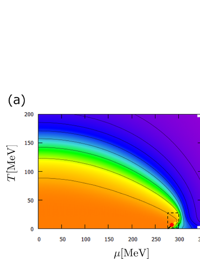
Figure 2: (a) Contour map of the chiral condensate in a wide region. (b) Enlargement of the region surrounded by dotted lines in (a). The filled circle (red) is the critical point and the solid (black) line is the first-order phase boundary.

At the QCD critical point, the chiral susceptibility diverges. Therefore, we locate the critical point by searching for the point where the sigma screening mass $M_{\sigma}$, the square of which is the inverse of the chiral susceptibility, becomes the smallest: We seek the minimum position of $M_{\sigma}$ using the data points where $M_{\sigma}$ is greater than $1\,\mathrm{MeV}$, because our choice of $k_{\mathrm{IR}}=1\,\mathrm{MeV}$ enables us to take into account fluctuations whose momentum scales are greater than $k_{\mathrm{IR}}$ so as to make the result of $M_{\sigma}$ reliable when $M_{\sigma}$ is larger than $1\,\mathrm{MeV}$. We also identify the first-order phase transition by a discontinuity of the chiral condensate. The results at $T=5.0\,\mathrm{MeV}$, $5.1\,\mathrm{MeV}$, and $5.2\,\mathrm{MeV}$ are shown in Fig. 3 as functions of $\mu-\mu_{t}(T)$, where $\mu_{t}(T)$ is the transition chemical potential for each temperature determined by the minimum point of the sigma curvature mass and is found to be $\mu_{t}(5.0\,\mathrm{MeV})=286.517~{}02\,\mathrm{MeV}$, $\mu_{t}(5.1\,\mathrm{MeV})=286.686~{}00\,\mathrm{MeV}$, and $\mu_{t}(5.2\,\mathrm{MeV})=286.853~{}20\,\mathrm{MeV}$.

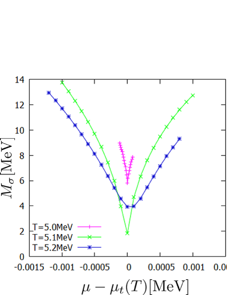
Figure 3: The sigma curvature masses and the chiral condensates at $T=5.0\,\mathrm{MeV}$, $5.1\,\mathrm{MeV}$, and $5.2\,\mathrm{MeV}$ as functions of $\mu-\mu_{t}(T)$.

We find that the sigma screening mass becomes smallest between $T=5.0\,\mathrm{MeV}$ and $T=5.2\,\mathrm{MeV}$ and between $\mu=\mu_{t}(5.0\,\mathrm{MeV})$ and $\mu=\mu_{t}(5.2\,\mathrm{MeV})$. Therefore, the critical temperature $T_{c}$ and the critical chemical potential $\mu_{c}$ are estimated as $T_{c}=5.1\pm 0.1\,\mathrm{MeV}$ and $\mu_{c}=286.6\pm 0.2\,\mathrm{MeV}$. The position of the critical point is quite different from the $(T,\mu)=(10\,\mathrm{MeV},292.97\,\mathrm{MeV})$ given in Ref. Tripolt:2014wra . Such a difference may be attributed to the different choice of $k_{\mathrm{IR}}$. In the following discussion, we regard $T_{c}$ and $\mu_{c}$ as $5.1\,\mathrm{MeV}$ and $286.686\,\mathrm{MeV}$, respectively. As seen in the behavior of the chiral condensate shown in the right panel of Fig. 3, the phase transition along the chemical potential is of first order when $T=5.0\,\mathrm{MeV}$ and a crossover when $T=5.2\,\mathrm{MeV}$.

It is known Kunhiro:1991 that the quark-number susceptibility $\chi_{q}\equiv\partial\rho_{q}/\partial\mu$ is coupled to the scalar susceptibility at finite $\mu$ and can be used to reveal the nature of the phase transition, where $\rho_{q}$ denotes the quark-number density. Indeed $\chi_{q}$ shows a singular behavior at the critical point, and hence an enhancement of $\chi_{q}$ is a useful measure of the critical region. We thus calculate $\chi_{q}$ to map out the critical region, as was done in Refs. Hatta:2002sj ; Kamikado:2012cp .

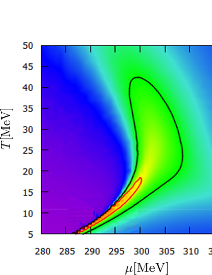
Figure 4: Contour map of the quark-number susceptibility near the critical point. The values are normalized with those of a free quark gas. The bold (black) line is the contour line of value 3 and the thin (red) line is that of value 6.

$\chi_{q}$ in the FRG formalism is calculated as follows. The effective action $\Gamma[\overline{\psi},\psi,\sigma,\vec{\pi}]$ in the finite-temperature formalism is related to the thermodynamic potential $\Omega$ as $T\Gamma[0,0,\sigma_{0},\vec{0}]=\Omega$ under the assumption that the chiral condensate is homogeneous and $\langle\vec{\pi}\rangle=\vec{0}$, which in our case reads

$$\frac{\Omega}{V}=U_{k\rightarrow 0}(\sigma_{0}^{2})-c\sigma_{0}.$$ (35)

The quark-number susceptibility $\chi_{q}$ is given by differentiating Eq. (35) twice with respect to the chemical potential:

$$\chi_{q}=-\frac{\partial^{2}}{\partial\mu^{2}}\left(U_{k\rightarrow 0}(\sigma_{0}^{2})-c\sigma_{0}\right).$$ (36)

We carry out the derivatives numerically. Figure 4 shows the contour map of the quark-number susceptibility, normalized by the value for the massless free quark gas:

$$\chi_{q}=\frac{2N_{c}N_{f}}{6}\left[T^{2}+\frac{3\mu^{2}}{\pi^{2}}\right].$$ (37)

3.3 Spectral function in the $\sigma$ channel away from the critical point

Before entering into discussions on the spectral properties in the meson channel near the critical point, we first show the numerical result of the spectral function $\rho_{\sigma}(\omega,p)$ in the sigma channel away from the critical point in the hadronic and QGP phases so that the peculiar behavior of the spectral functions near the critical point shown in the next subsection shall be prominent.

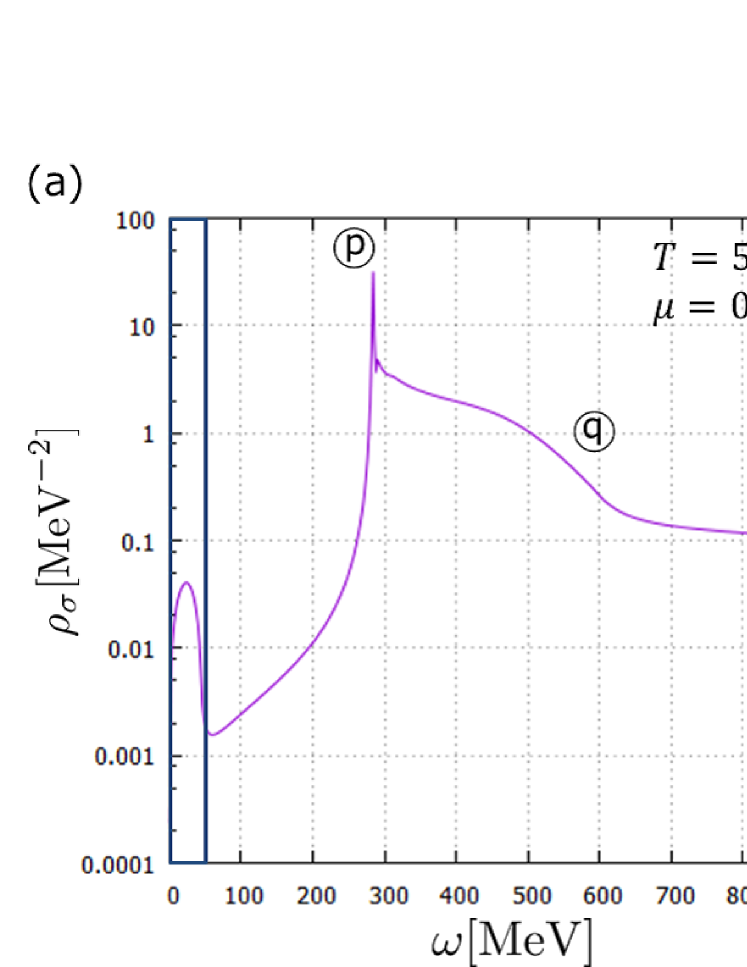
Figure 5: (a) The spectral function in the $\sigma$ channel in the hadronic phase at ($T=50\,\mathrm{MeV}$,  $\mu=0\,\mathrm{MeV}$). (b) The same as (a) in the QGP phase at ($T=50\,\mathrm{MeV}$,  $\mu=400\,\mathrm{MeV}$). The spatial momentum is set to $p=50\,\mathrm{MeV}$, and the inside of the blue box in each figure is the space-like region ($\omega\,<\,p$). The positions of the thresholds for the $2\sigma$, $2\pi$, and $\overline{\psi}\psi$ decay channels determined by Eq. (38) are denoted by ⓢ, ⓟ, and ⓠ.

Figures 5(a) and 5(b) show $\rho_{\sigma}(\omega,p)$ at $p\equiv|\vec{p}|=50$ MeV for ($T=50$ MeV, $\mu=0$ MeV) and ($T=50$ MeV, $\mu=400$ MeV), respectively: The former (latter) is in the hadronic (QGP) phase. In the former case, there is a sharp peak at $\omega=290\,\mathrm{MeV}$ and a relatively small bump in the space-like region $\omega<p$; these correspond to the sigma meson with a modified mass at finite temperature and the phonon mode composed of particle–hole excitations, respectively, which is in accord with the result in the RPA in Ref. Fujii:2004jt .

The spectral function also tells us the decay and absorption processes of the particle excitations from the width of the corresponding peaks or bumps. In our energy scale, the following processes contribute to the spectral function $\rho_{\sigma}(\omega,\vec{p})$:

$$\sigma^{\ast}\rightarrow\sigma\sigma,\quad\sigma^{\ast}\rightarrow\pi\pi,\quad\sigma^{\ast}\rightarrow\overline{\psi}\psi,\quad\sigma^{\ast}\sigma\rightarrow\sigma,\quad\sigma^{\ast}\pi\rightarrow\pi,\quad\sigma^{\ast}\psi\rightarrow\psi,$$

where $\sigma^{\ast}$ denotes a virtual state in the sigma channel with energy–momentum $(\omega,\vec{p})$. The energy–momentum conservation gives constraints on the possible $(\omega,\,\vec{p})$ region for the first three processes as follows:

$$\omega\geq\sqrt{\vec{p}^{2}+(2M_{\sigma})^{2}}\ \ \text{for}\ \ \sigma^{\ast}\rightarrow\sigma\sigma,$$

$$\omega\geq\sqrt{\vec{p}^{2}+(2M_{\pi})^{2}}\ \ \text{for}\ \ \sigma^{\ast}\rightarrow\pi\pi,$$ (38)

$$\omega\geq\sqrt{\vec{p}^{2}+(2M_{\psi})^{2}}\ \ \text{for}\ \ \sigma^{\ast}\rightarrow\overline{\psi}\psi,$$

which are all in the time-like region. On the other hand, the second three processes are all collisional ones and possible only in the space-like region, $0\leq\omega<p$. In particular, the last process $\sigma^{\ast}\psi\rightarrow\psi$ corresponds to the absorption process of the $\sigma^{\ast}$ mode into a thermally excited quark. In short, the width of the large bump at $\omega=290\,\mathrm{MeV}$ in Fig. 5(a) comes from the $2\pi$ decay process, while the small bump arises from the space-like processes.

In the latter case, at $T=50\,\mathrm{MeV}$ and $\mu=400\,\mathrm{MeV}$, the peak position corresponding to the sigma meson is shifted to $\omega=210\,\mathrm{MeV}$, while the bump of the particle–hole excitations still persists in the space-like region.

3.4 Spectral functions near the QCD critical point

Figure 6: The spectral functions in the $\sigma$ channel near the QCD critical point. The temperature is fixed to $T_{c}$. The spatial momentum is set to $p=50\,\mathrm{MeV}$ and the inside of the blue box in each figure is the space-like region. The results in $286.00\,\mathrm{MeV}\leq\mu\leq 286.57\,\mathrm{MeV}$ are shown in (a) and the results in $286.57\,\mathrm{MeV}\leq\mu\leq 286.59\,\mathrm{MeV}$ are shown in (b). The position of the $2\sigma$ decay threshold for each chemical potential is denoted by ⓢ. The $2\pi$ and $\overline{\psi}\psi$ decay thresholds hardly change and are represented by ⓟ and ⓠ.

We calculate the spectral function in the $\sigma$ channel near the QCD critical point, by increasing the chemical potential toward $\mu_{c}$ along a constant temperature line $T=T_{c}$. The results at $\mu=286.00\,\mathrm{MeV}$, $\mu=286.50\,\mathrm{MeV}$, and $\mu=286.57\,\mathrm{MeV}$ are shown in Fig. 6 (a). One can see the sigma-mesonic peak as well as bumps corresponding to $2\sigma$ and $2\pi$ decay in the time-like region. The peak position of the sigma-mesonic mode shifts to lower energy as the system approaches the critical point. The position of the $2\sigma$ threshold also shifts to a lower energy while those of the $2\pi$ and $\overline{\psi}\psi$ thresholds hardly change. The spectral function in the space-like region is drastically enhanced as the system is close to the critical point. This behavior can be interpreted as the softening of the particle–hole mode, which is in accordance with the result in Ref. Fujii:2004jt . In Fig. 6(b), we show the results at chemical potentials much closer to the critical point. Because of numerical instability in $286.60\,\mathrm{MeV}\leq\mu\lesssim 360\,\mathrm{MeV}$, we choose $\mu=286.58\,\mathrm{MeV}$ and $\mu=286.59\,\mathrm{MeV}$. For comparison, the result at $\mu=286.57\,\mathrm{MeV}$ is also shown. These results are drastically different from those in $\mu\leq 286.57\,\mathrm{MeV}$. In $\mu>286.57\,\mathrm{MeV}$, the peak of the sigma-mesonic mode penetrates into the space-like region and then merges into the particle–hole mode.

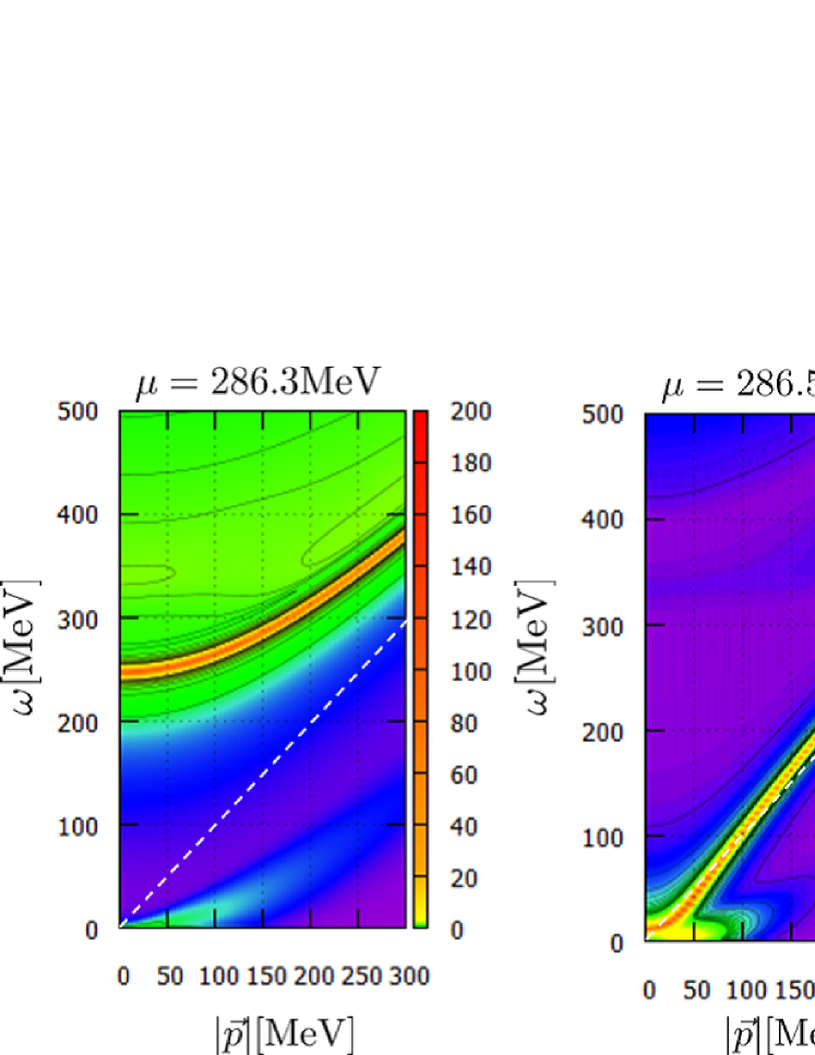
Figure 7: Contour maps of $\rho_{\sigma}$ at $T=T_{c}$ and $\mu=286.3\mathrm{MeV}$, $286.575\mathrm{MeV}$, and $286.59\mathrm{MeV}$.

We can see the dispersion relations of the modes by making contour maps of the spectral functions as functions of $\omega$ and $p$. Figure 7 shows the dispersion relations of the sigma-meson and particle–hole modes near the critical point. At $\mu=286.3\,\mathrm{MeV}$, the sigma-mesonic peaks can be seen in the time-like region as well as the particle–hole bump in the space-like region. As the chemical potential increases, the dispersion relation of the sigma-mesonic mode shifts downward and it touches the light cone near $\mu=286.575\,\mathrm{MeV}$. At $\mu=286.59\,\mathrm{MeV}$, in the low-momentum region the sigma-mesonic mode clearly penetrates into the space-like region and merges with the particle–hole bump, which has a flat dispersion relation in the low-momentum region. Our results indicate that the sigma-mesonic mode as well as the particle–hole mode can become soft near the critical point.

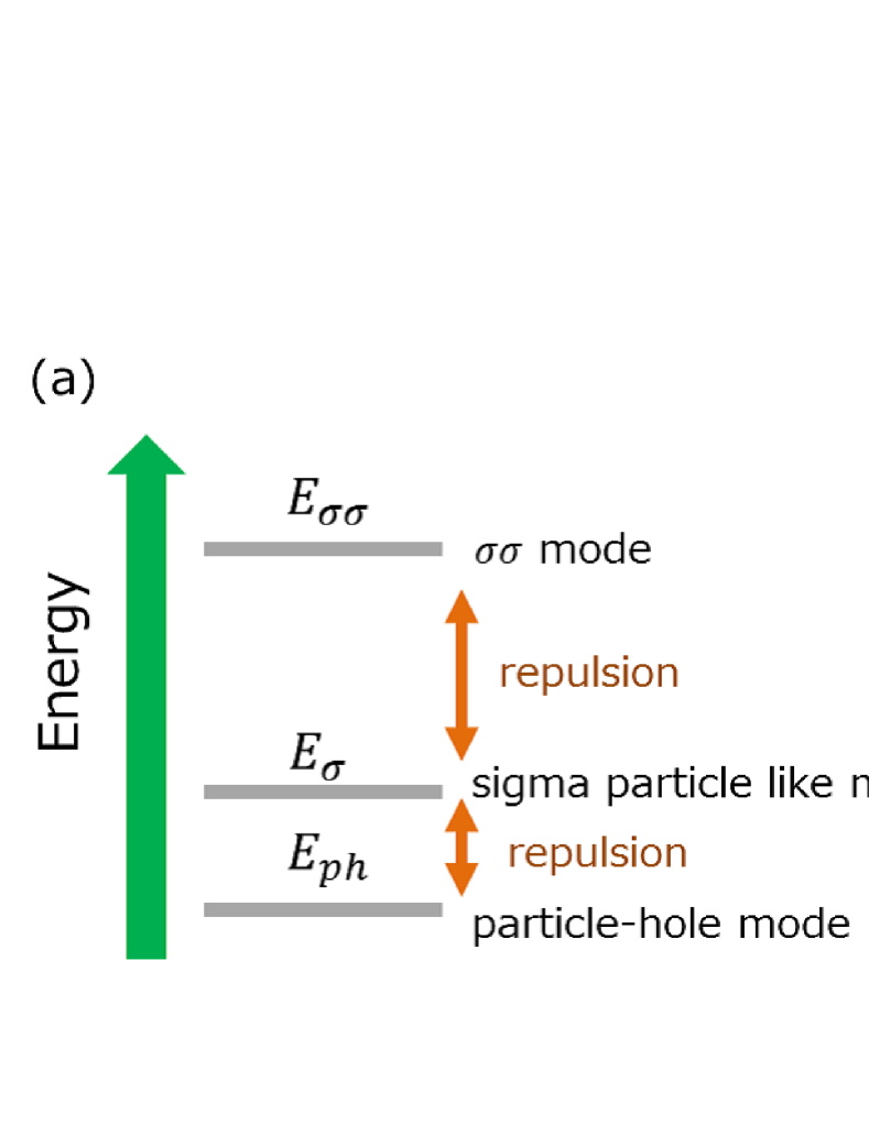
Figure 8: (a) Conceptual picture of level repulsion of the sigma-mesonic mode, $2\sigma$ mode, and particle–hole mode. (b) The spectral functions in the $\sigma$ channel with a substituted three-point vertex $a\Gamma_{k,\sigma\sigma\sigma}^{(3)}$ at $T=T_{c}$, $\mu=286.57\,\mathrm{MeV}$, and $p=50\,\mathrm{MeV}$. The inside of the blue box is the space-like region.

One of the possible triggers of this phenomenon is the level repulsion between the sigma-mesonic mode and other modes. In particular, the two-sigma ($\sigma\sigma$) mode is considered to play an important role in the level repulsion since the threshold of the two-sigma mode shifts downward as the system approaches the critical point. Let us suppose that the particle–hole mode, the sigma-mesonic mode, and the two-sigma mode can each be described by a state having a single energy level. Then the system can be regarded as a three-level system, as depicted in Fig. 8 (a): The interaction within the three states leads to a level repulsion: If the interaction between the $\sigma$-mesonic mode and the $\sigma\sigma$ state becomes sufficiently strong as the system approaches the critical point, the energy level of the sigma meson will be so strongly pushed down that it penetrates into the space-like region. To show that this scenario can be the case, we change the strength of the three-point vertex $\Gamma_{k,\sigma\sigma\sigma}^{(0,3)}$ by hand to investigate the behavior of the sigma-meson peak. The results in the cases of multiplying $\Gamma_{k,\sigma\sigma\sigma}^{(0,3)}$ by factors $0.8$ and $1.02$ are shown in Fig. 8 (b). The position of the sigma meson goes up when the three-point vertex is weakened, whereas it exhibits a downward shift to a lower energy when the three-point vertex is slightly enhanced. This result suggests that the above interpretation in terms of a level repulsion can be correct.

Here it should be noted that our results exhibit a superluminal group velocity of the sigma-mesonic mode near the critical point, as seen in Fig. 7 for $p=100\,\mathrm{MeV}$ at $\mu=286.59\,\mathrm{MeV}$. Such an unphysical extreme behavior may be an artifact of our truncation scheme, in which some of the higher-order terms in the derivative expansion, such as the wave-function renormalization and so on, are neglected, although a drastic softening of the sigma-mesonic mode may be true. Conversely speaking, such a drawback could disappear if one uses improved methods with higher-derivative terms being incorporated. One of the most important improvements is the inclusion of wave-function renormalization Helmboldt:2014iya ; Kamikado:2013pya , since this may become important when additional modes emerge. However, this task is beyond the scope of the present work and will be left as a future project.

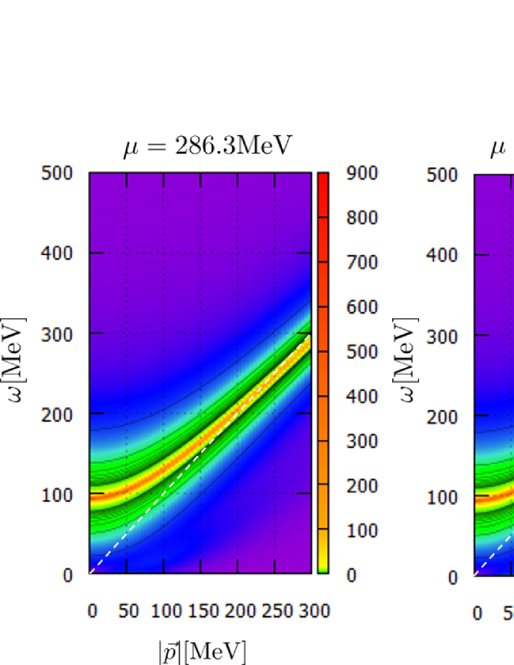
Figure 9: Contour maps of $\rho_{\pi}$ at $T=T_{c}$ and $\mu=286.3\,\mathrm{MeV}$, $286.575\,\mathrm{MeV}$, and $286.59\,\mathrm{MeV}$.

So far, we have concentrated on the spectral function in the sigma channel and seen interesting behaviors of it near the critical point. It would be intriguing to examine whether the spectral function $\rho_{\pi}(\omega,p)$ in the pion channel shows any peculiar behavior near the critical point. The numerical result of $\rho_{\pi}(\omega,p)$ near the critical point is shown in Fig. 9, from which one can clearly see the dispersion relation of the pion mode in the time-like region but not in the space-like region. In contrast to $\rho_{\sigma}$, $\rho_{\pi}$ hardly changes near the critical point, indicating that there is no critical behavior in the isovector pseudoscalar modes in either the space-like or time-like region. This different critical behavior in the sigma and pion channels may be understood as follows: First of all, the finite current quark mass makes the would-be chiral transition cease to be of second order, and hence prevents the quartet mesons composed of the sigma meson and pion from becoming soft modes inherent in the second-order transition, as mentioned in Sect. 1. However, the finite chemical potential $\mu\not=0$ makes scalar–vector coupling possible and the critical point can get to exist with the $Z_{2}$ universality class of the second-order transition. Thus the soft modes inherent for the second-order transition appear due to the very scalar–vector coupling in the space-like region, which is primarily composed of particle–hole excitations. In principle, the pion is coupled to fluctuations in the isovector pseudoscalar or axial vector channels, which are reduced to spin–isospin modes in the nonrelativistic limitMigdal:1978az . Our result simply shows that such pionic modes do not develop in the space-like region at least around the critical point. In the scalar channel, the coupling of the single and double sigma modes is so strong that a level repulsion between them drastically lowers the energy of the sigma-mesonic mode in the time-like region. In contrast to the scalar channel, the coupling of the single pion mode to other modes, such as the mode that consists of one sigma and one pion, would not be strong enough to cause the softening behavior of the isovector pseudoscalar mode in the time-like region.

4 Summary

We have calculated the spectral functions in the meson channels in the quark–meson model with the functional renormalization group method based on the local potential approximation (LPA). A particular emphasis is put on the behavior of the spectral function in the $\sigma$ channel near the QCD critical point. Our results show that the particle–hole mode (phonon) is enhanced near the critical point, and thus imply that the density fluctuations are soft modes at the critical point, as was suggested in the RPA using the NJL model Fujii:2004jt . In addition, we have found that the low-energy dispersion curve of the sigma meson penetrates into the space-like region and the mode merges into the particle–hole mode near the critical point. This result may imply that the sigma meson also acts as a soft mode at the QCD critical point. We have also suggested that a possible level repulsion between the sigma meson and the two-sigma state leads to the anomalous softening of the sigma meson: An artificial variation of the strength of the $\sigma$ three-point vertex $\Gamma_{k,\sigma\sigma\sigma}^{(0,3)}$ strongly affects the position of the sigma meson. We have also investigated the spectral function in the pion channel near the critical point, which shows no softening in either the time-like region or the space-like region, in contrast to the isoscalar modes.

Since our result might provide a new picture in which the critical dynamics at the QCD critical point can be described by an effective theory composed of not only the hydrodynamical modes including the density fluctuation but also the sigma-meson mode, there might be some implications for the dynamical class of the QCD critical point Son:2004iv ; Stephanov:1999zu ; Berdnikov:1999ph .

In recent years, the possible existence of inhomogeneous chiral phases in dense quark matter has been intensively examined Nakano:2004cd ; Nickel:2009wj ; Nickel:2009ke ; Muller:2013tya . It would be interesting to investigate in the FRG how the existence of the inhomogeneous phases affects the behavior of low-energy modes, including the Nambu–Goldstone modes. It is also worth emphasizing that our analysis of the spectral functions in the space-like region or particle–hole modes can be extended to that of precursors of such inhomogeneous phases: our results showing the softening and nonsoftening of the particle–hole modes in the sigma and pion channels might imply that the inhomogeneous phase with pion condensate does not come into existence as a result of a second-order transition.

Our calculation is based on the local potential approximation, in which some of the higher-order terms in the derivative expansion are neglected. Such a simple truncation scheme might be an origin of a superluminal group velocity in the close vicinity of the critical point encountered in Sect. 3. Thus, it is imperative to confirm the results by employing improved methods incorporating higher-derivative terms, including the wave-function renormalization, since it is important to identify when composite collective modes emerge. This intriguing task will, however, be left for future work.

Appendix A The explicit forms of loop-functions after Matsubara summations

In this appendix, we show the explicit forms of Eqs. (18)–(20) after Matsubara summation. The momentum integral of $I^{(2)}_{\alpha}$ can be calculated easily and its form is given as follows:

$$I^{(2)}_{\alpha}=\frac{k^{4}}{6\pi^{2}}\left(\frac{1+2n_{B}(E_{\alpha})}{2E_{\alpha}^{3}}-\frac{n_{B}^{\prime}(E_{\alpha})}{E_{\alpha}^{2}}\right),$$ (39)

where $E_{\alpha}=\sqrt{k^{2}+m_{\alpha}^{2}}$ and $n_{B,F}^{\prime}(E)=\frac{dn_{B,F}(E)}{dE}$.

Next, we show the forms of $J_{k,\alpha\alpha}(P)$ and $J_{k,\overline{\psi}\psi}^{(\sigma)}(P)$ after Matsubara summation. $J_{k,\alpha\alpha}(P)$ ($J_{k,\overline{\psi}\psi}^{(\sigma)}(P)$) has regulators with different arguments: $R_{k}^{B}(Q)$ and $R_{k}^{B}(Q-P)$ ($R_{k}^{F}(Q)$ and $R_{k}^{F}(Q-P)$). These regulators contain the Heaviside step functions such that the momentum dependence of the integrands differs between the two integral regions $D_{1}$ and $D_{2}$:

$$D_{1} =\left\{\left.\vec{q}\in\mathbb{R}^{3}\right||\vec{q}-\vec{p}|<k\ \text{and}\ |\vec{q}|<k\right\},$$

$$D_{2} =\left\{\left.\vec{q}\in\mathbb{R}^{3}\right||\vec{q}-\vec{p}|<k\ \text{and}\ |\vec{q}|>k\right\}.$$

Using the following notations,

$$\tilde{E}_{\alpha}=\sqrt{\vec{q}^{2}+M_{\alpha}^{2}},\ \ \ \ \cos\varphi=\frac{\vec{q}\cdot(\vec{q}-\vec{p})}{\left|\vec{q}\right|\left|\vec{q}-\vec{p}\right|},$$

we show the forms of $J_{k,\alpha\alpha}(P)$ and $J^{(\sigma)}_{k,\bar{\psi}\psi}(P)$ after Matsubara summation below:

$$J_{k,\alpha\beta}(P)= \int_{D_{1}}\frac{d^{3}q}{\left(2\pi\right)^{3}}\frac{k}{2}\left[(1+n_{B}(E_{\alpha}))\frac{E_{\alpha}^{2}+E_{\beta}^{2}-(2E_{\alpha}+\mathrm{i}p_{0})^{2}}{E_{\alpha}^{3}(E_{\beta}^{2}-(E_{\alpha}+\mathrm{i}p_{0})^{2})^{2}}+n_{B}(E_{\alpha})\frac{E_{\alpha}^{2}+E_{\beta}^{2}-(2E_{\alpha}-\mathrm{i}p_{0})^{2}}{E_{\alpha}^{3}(E_{\beta}^{2}-(E_{\alpha}-\mathrm{i}p_{0})^{2})^{2}}\right.$$

$$+\frac{2(1+n_{B}(E_{\beta}))}{E_{\beta}(E_{\alpha}^{2}-(E_{\beta}-\mathrm{i}p_{0})^{2})^{2}}+\frac{2n_{B}(E_{\beta})}{E_{\beta}(E_{\alpha}^{2}-(E_{\beta}+\mathrm{i}p_{0})^{2})^{2}}$$

$$\left.-\frac{n_{B}^{\prime}(E_{\alpha})}{E_{\alpha}^{2}(E_{\beta}^{2}-(E_{\alpha}-\mathrm{i}p_{0})^{2})}-\frac{n_{B}^{\prime}(E_{\alpha})}{E_{\alpha}^{2}(E_{\beta}^{2}-(E_{\alpha}+\mathrm{i}p_{0})^{2})}\right]$$

$$+\int_{D_{2}}\frac{d^{3}q}{\left(2\pi\right)^{3}}\frac{k}{2}\left[(1+n_{B}(E_{\alpha}))\frac{E_{\alpha}^{2}+\tilde{E}_{\beta}^{2}-(2E_{\alpha}+\mathrm{i}p_{0})^{2}}{E_{\alpha}^{3}(\tilde{E}_{\beta}^{2}-(E_{\alpha}+\mathrm{i}p_{0})^{2})^{2}}+n_{B}(E_{\alpha})\frac{E_{\alpha}^{2}+\tilde{E}_{\beta}^{2}-(2E_{\alpha}-\mathrm{i}p_{0})^{2}}{E_{\alpha}^{3}(\tilde{E}_{\beta}^{2}-(E_{\alpha}-\mathrm{i}p_{0})^{2})^{2}}\right.$$

$$+\frac{2(1+n_{B}(\tilde{E}_{\beta}))}{\tilde{E}_{\beta}(E_{\alpha}^{2}-(\tilde{E}_{\beta}-\mathrm{i}p_{0})^{2})^{2}}+\frac{2n_{B}(\tilde{E}_{\beta})}{\tilde{E}_{\beta}(E_{\alpha}^{2}-(\tilde{E}_{\beta}+\mathrm{i}p_{0})^{2})^{2}}$$

$$\left.-\frac{n_{B}^{\prime}(E_{\alpha})}{E_{\alpha}^{2}(\tilde{E}_{\beta}^{2}-(E_{\alpha}-\mathrm{i}p_{0})^{2})}-\frac{n_{B}^{\prime}(E_{\alpha})}{E_{\alpha}^{2}(\tilde{E}_{\beta}^{2}-(E_{\alpha}+\mathrm{i}p_{0})^{2})}\right],$$ (40)

$$J^{(\sigma)}_{k,\bar{\psi}\psi}(P)= J^{(\pi)}_{k,\overline{\psi}\psi}(P)+\int_{D_{1}}\frac{d^{3}q}{(2\pi)^{3}}4m_{\psi}^{2}g_{s}^{2}k\left[(1-n_{F}(E_{\psi}-\mu)-n_{F}(E_{\psi}+\mu))\frac{12E_{\psi}^{2}+p_{0}^{2}}{E_{\psi}^{3}(4E_{\psi}^{2}+p_{0}^{2})^{2}}\right.$$

$$\left.-n_{F}^{\prime}(E_{\psi}-\mu)\frac{1}{\mathrm{i}p_{0}E_{\psi}^{2}(2E_{\psi}+\mathrm{i}p_{0})}+n_{F}^{\prime}(E_{\psi}+\mu)\frac{1}{\mathrm{i}p_{0}E_{\psi}^{2}(2E_{\psi}-\mathrm{i}p_{0})}\right]$$

$$+\int_{D_{2}}\frac{d^{3}q}{(2\pi)^{3}}4m_{\psi}^{2}g_{s}^{2}k\left[(1-n_{F}(E_{\psi}-\mu))\frac{(2E_{\psi}-\mathrm{i}p_{0})^{2}-6E_{\psi}^{2}-k^{2}+2p_{0}^{2}+\vec{q}^{2}}{E_{\psi}^{3}(\tilde{E}_{\psi}^{2}-(E_{\psi}+\mathrm{i}p_{0})^{2})^{2}}\right.$$

$$-n_{F}(E_{\psi}+\mu)\frac{(2E_{\psi}+\mathrm{i}p_{0})^{2}-6E_{\psi}^{2}-k^{2}+2p_{0}^{2}+\vec{q}^{2}}{E_{\psi}^{3}(\tilde{E}_{\psi}^{2}-(E_{\psi}-\mathrm{i}p_{0})^{2})^{2}}$$

$$+\frac{n_{F}^{\prime}(E_{\psi}-\mu)}{E_{\psi}^{2}(\tilde{E}_{\psi}^{2}-(E_{\psi}+\mathrm{i}p_{0})^{2})}+\frac{n_{F}^{\prime}(E_{\psi}+\mu)}{E_{\psi}^{2}(\tilde{E}_{\psi}^{2}-(E_{\psi}-\mathrm{i}p_{0})^{2})}$$

$$\left.+\frac{2(1-n_{F}(\tilde{E}_{\psi}-\mu))}{\tilde{E}_{\psi}(E_{\psi}^{2}-(\tilde{E}_{\psi}-\mathrm{i}p_{0})^{2})^{2}}-\frac{2n_{F}(\tilde{E}_{\psi}+\mu)}{\tilde{E}_{\psi}(E_{\psi}^{2}-(\tilde{E}_{\psi}+\mathrm{i}p_{0})^{2})^{2}}\right],$$ (41)

$$J^{(\pi)}_{k,\overline{\psi}\psi}(P)= \int_{D_{1}}\frac{d^{3}q}{(2\pi)^{3}}\left(-2g_{s}^{2}k\right)\left[(1-n_{F}(E_{\psi}-\mu)-n_{F}(E_{\psi}+\mu))\frac{16E_{\psi}^{4}-k^{2}(12E_{\psi}^{2}+p_{0}^{2})}{E_{\psi}^{3}(4E_{\psi}^{2}+p_{0}^{2})^{2}}\right.$$

$$\left.+n_{F}^{\prime}(E_{\psi}-\mu)\frac{k^{2}+\mathrm{i}p_{0}E_{\psi}}{\mathrm{i}p_{0}E_{\psi}^{2}(2E_{\psi}+\mathrm{i}p_{0})}-n_{F}^{\prime}(E_{\psi}+\mu)\frac{k^{2}-\mathrm{i}p_{0}E_{\psi}}{\mathrm{i}p_{0}E_{\psi}^{2}(2E_{\psi}-\mathrm{i}p_{0})}\right]$$

$$+\int_{D_{1}}\frac{d^{3}q}{(2\pi)^{3}}\cos\varphi\left(-2g_{s}^{2}k\right)\left[(1-n_{F}(E_{\psi}-\mu)-n_{F}(E_{\psi}+\mu))\frac{-8E_{\psi}^{4}+2E_{\psi}^{2}(6k^{2}-p_{0}^{2})+k^{2}p_{0}^{2}}{E_{\psi}^{3}(4E_{\psi}^{2}+p_{0}^{2})^{2}}\right.$$

$$\left.-\frac{k^{2}n_{F}^{\prime}(E_{\psi}-\mu)}{\mathrm{i}p_{0}E_{\psi}^{2}(2E_{\psi}+\mathrm{i}p_{0})}+\frac{k^{2}n_{F}^{\prime}(E_{\psi}+\mu)}{\mathrm{i}p_{0}E_{\psi}^{2}(2E_{\psi}-\mathrm{i}p_{0})}\right]$$

$$+\int_{D_{2}}\frac{d^{3}q}{(2\pi)^{3}}\left(-2g_{s}^{2}k\right)\left[(1-n_{F}(E_{\psi}-\mu))\frac{-2\mathrm{i}p_{0}E_{\psi}^{3}+4\mathrm{i}p_{0}k^{2}E_{\psi}-k^{2}(p_{0}^{2}-k^{2}+\vec{q}^{2})+2\vec{q}^{2}E_{\psi}^{2}}{E_{\psi}^{3}(\tilde{E}_{\psi}^{2}-(E_{\psi}+\mathrm{i}p_{0})^{2})^{2}}\right.$$

$$+n_{F}(E_{\psi}+\mu)\frac{-2\mathrm{i}p_{0}E_{\psi}^{3}+4\mathrm{i}p_{0}k^{2}E_{\psi}+k^{2}(p_{0}^{2}-k^{2}+\vec{q}^{2})-2\vec{q}^{2}E_{\psi}^{2}}{E_{\psi}^{3}(\tilde{E}_{\psi}^{2}-(E_{\psi}-\mathrm{i}p_{0})^{2})^{2}}$$

$$-n_{F}^{\prime}(E_{\psi}-\mu)\frac{k^{2}+\mathrm{i}p_{0}E_{\psi}}{E_{\psi}^{2}(\tilde{E}_{\psi}^{2}-(E_{\psi}+\mathrm{i}p_{0})^{2})}-n_{F}^{\prime}(E_{\psi}+\mu)\frac{k^{2}-\mathrm{i}p_{0}E_{\psi}}{E_{\psi}^{2}(\tilde{E}_{\psi}^{2}-(E_{\psi}-\mathrm{i}p_{0})^{2})}$$

$$\left.-(1-n_{F}(\tilde{E}_{\psi}-\mu))\frac{2(\vec{q}^{2}-\mathrm{i}p_{0}\tilde{E}_{\psi})}{\tilde{E}_{\psi}(E_{\psi}^{2}-(\tilde{E}_{\psi}-\mathrm{i}p_{0})^{2})^{2}}+n_{F}(\tilde{E}_{\psi}+\mu)\frac{2(\vec{q}^{2}+\mathrm{i}p_{0}\tilde{E}_{\psi})}{\tilde{E}_{\psi}(E_{\psi}^{2}-(\tilde{E}_{\psi}+\mathrm{i}p_{0})^{2})^{2}}\right]$$

$$+\int_{D_{2}}\frac{d^{3}q}{(2\pi)^{3}}\cos\varphi\left(-2g_{s}^{2}k\right)|\vec{q}|$$

$$\times\left[(1-n_{F}(E_{\psi}-\mu))\frac{2\mathrm{i}p_{0}E_{\psi}^{3}-4\mathrm{i}p_{0}E_{\psi}k^{2}+k^{2}(p_{0}^{2}-k^{2}+\vec{q}^{2})-E_{\psi}^{2}(k^{2}+p_{0}^{2}+\vec{q}^{2})}{E_{\psi}^{3}k(\tilde{E}_{\psi}^{2}-(E_{\psi}+\mathrm{i}p_{0})^{2})^{2}}\right.$$

$$+n_{F}(E_{\psi}+\mu)\frac{2\mathrm{i}p_{0}E_{\psi}^{3}-4\mathrm{i}p_{0}E_{\psi}k^{2}-k^{2}(p_{0}^{2}-k^{2}+\vec{q}^{2})+E_{\psi}^{2}(k^{2}+p_{0}^{2}+\vec{q}^{2})}{E_{\psi}^{3}k(\tilde{E}_{\psi}^{2}-(E_{\psi}-\mathrm{i}p_{0})^{2})^{2}}$$

$$+\frac{kn_{F}^{\prime}(E_{\psi}-\mu)}{E_{\psi}^{2}(\tilde{E}_{\psi}^{2}-(E_{\psi}+\mathrm{i}p_{0})^{2})}+\frac{kn_{F}^{\prime}(E_{\psi}+\mu)}{E_{\psi}^{2}(\tilde{E}_{\psi}^{2}-(E_{\psi}-\mathrm{i}p_{0})^{2})}$$

$$\left.+(1-n_{F}(\tilde{E}_{\psi}-\mu))\frac{k^{2}-p_{0}^{2}+\vec{q}^{2}-2\mathrm{i}p_{0}\tilde{E}_{\psi}}{k\tilde{E}_{\psi}(E_{\psi}^{2}-(\tilde{E}_{\psi}-\mathrm{i}p_{0})^{2})^{2}}-n_{F}(\tilde{E}_{\psi}+\mu)\frac{k^{2}-p_{0}^{2}+\vec{q}^{2}+2\mathrm{i}p_{0}\tilde{E}_{\psi}}{k\tilde{E}_{\psi}(E_{\psi}^{2}-(\tilde{E}_{\psi}+\mathrm{i}p_{0})^{2})^{2}}\right],$$ (42)

for which the external Matsubara frequency $ip_{0}$ is to be replaced to make analytic continuation.

Appendix B Numerical stability conditions for solving the flow equation of the effective potential

In general when one solves a partial differential equation numerically, the discretization of derivatives may cause numerical instability. Thus, one needs to impose numerical stability conditions to avoid the enhancement of the error due to accumulation. The derivation of such conditions is concretely demonstrated in the case of linear partial differential equations and briefly mentioned in the case of nonlinear partial differential equations in Ref. NumericalRecipes . In this appendix we consider the numerical stability conditions for a nonlinear partial differential equation that is a generalized equation of Eq. (14) to derive the numerical stability conditions for solving Eq. (14) in the grid method.

Consider a nonlinear partial differential equation for some function $u(t,\sigma)$ of the following form:

$$\frac{\partial u(t,\sigma)}{\partial t}=f\left(t,\sigma,u(t,\sigma),\frac{\partial u(t,\sigma)}{\partial\sigma},\frac{\partial^{2}u(t,\sigma)}{\partial\sigma^{2}}\right),$$ (43)

where $f$ is an arbitrary real function. This equation is a generalized equation of Eq. (14). We derive the numerical stability conditions for this equation in the case of the forward difference for the $t$-derivative and the central three-point difference for the $\sigma$-derivative. We expect that the derived conditions can also be applied to the fourth-order Runge–Kutta method that we use in the practical calculations. Then the discretized flow equation leads

$$\frac{u(t+\Delta t,\sigma)-u(t,\sigma)}{\Delta t}$$

$$=f\left(t,\sigma,u(t,\sigma),\frac{u(t,\sigma+\Delta\sigma)-u(t,\sigma-\Delta\sigma)}{2\Delta\sigma},\frac{u(t,\sigma+\Delta\sigma)-2u(t,\sigma)+u(t,\sigma-\Delta\sigma)}{{(\Delta\sigma)}^{2}}\right),$$ (44)

where $\Delta t$ and $\Delta\sigma$ are intervals of discretization of $t$ and $\sigma$. We suppose that some numerical error occurs at some step of the numerical calculation and $u(t,\sigma)$ is written as follows:

$$u(t,\sigma)=u_{0}(t,\sigma)+\delta u(t,\sigma),$$ (45)

where $u_{0}(t,\sigma)$ is the exact solution of Eq. (44) and $\delta u(t,\sigma)$ is the deviation from the exact solution caused by numerical error. We substitute Eq. (45) into Eq. (44) and get the evolution equation for $\delta u(t,\sigma)$, considering the first order of expansion with $\delta u(t,\sigma)$ and using the fact that $u_{0}(t,\sigma)$ exactly satisfies Eq. (44):

$$\frac{\delta u(t+\Delta t,\sigma)-\delta u(t,\sigma)}{\Delta t} =F\left(t,\sigma,u_{0},\frac{\tilde{\partial}u_{0}}{\partial\sigma},\frac{\tilde{\partial}^{2}u_{0}}{\partial\sigma^{2}}\right)\frac{\delta u(t+\Delta t,\sigma)-\delta u(t-\Delta t,\sigma)}{2\Delta\sigma}$$

$$+G\left(t,\sigma,u_{0},\frac{\tilde{\partial}u_{0}}{\partial\sigma},\frac{\tilde{\partial}^{2}u_{0}}{\partial\sigma^{2}}\right)\frac{\delta u(t+\Delta t,\sigma)-2\delta u(t,\sigma)+\delta u(t-\Delta t,\sigma)}{{(\Delta\sigma)}^{2}},$$ (46)

where

$$F\equiv\frac{\partial f}{\partial u^{\prime}},\ G\equiv\frac{\partial f}{\partial u^{\prime\prime}}\ \left(u^{\prime}=\frac{\partial u}{\partial\sigma},u^{\prime\prime}=\frac{\partial^{2}u}{\partial\sigma^{2}}\right),$$

$$\frac{\tilde{\partial}u_{0}}{\partial\sigma}\equiv\frac{\delta u(t,\sigma+\Delta\sigma)-\delta u(t,\sigma-\Delta\sigma)}{2\Delta\sigma},\ \frac{\tilde{\partial}^{2}u_{0}}{\partial\sigma^{2}}\equiv\frac{\delta u(t,\sigma+\Delta\sigma)-2\delta u(t,\sigma)+\delta u(t,\sigma-\Delta\sigma)}{{(\Delta\sigma)}^{2}}.$$

For simplicity, we ignore the $\sigma$ dependence of $F$ and $G$. Then the solutions of Eq. (46) can be written as linear combinations of Fourier components:

$$\delta u(m\Delta t,n\Delta\sigma;k)=\xi_{k}(m\Delta t)e^{ikn\Delta\sigma},$$ (47)

where we substitute $m\Delta t$ and $n\Delta\sigma$ for $t$ and $\sigma$ ($m,n\in\mathbb{Z}$). By substituting Eq. (47) into Eq. (46), we get the following equation after some manipulation:

$$\frac{\xi_{k}((m+1)\Delta t)}{\xi_{k}(m\Delta t)}=1-\frac{2G\Delta t}{(\Delta\sigma)^{2}}(1-\cos k\Delta\sigma)+iF\frac{\Delta t}{\Delta\sigma}\sin(k\Delta\sigma).$$ (48)

If $|\xi_{k}((m+1)\Delta t)/\xi_{k}(m\Delta t)|>1$, the numerical deviation is amplified as $m$ increases (the flow step goes forward) and numerical instability occurs. Therefore, the condition for stable calculation is

$$\left|\frac{\xi_{k}((m+1)\Delta t)}{\xi_{k}(m\Delta t)}\right|\leq 1.$$ (49)

From Eq. (48), this condition can be rewritten as

$$h(X)\leq 1\ \ (-1\leq X\leq 1),$$ (50)

where $X\equiv\cos(k\Delta x)$ and $h(X)$ is defined as

$$h(X)\equiv(a^{2}-b^{2})X^{2}+2a(1-a)X+(1-a)^{2}+b^{2}\ \ \left(a=\frac{2G\Delta t}{(\Delta\sigma)^{2}},b=\frac{F\Delta t}{\Delta\sigma}\right).$$ (51)

Considering that $h(X)$ satisfies $h(1)=1$, one can easily understand that the condition Eq. (50) is equivalent to the following conditions:

$$\frac{dh}{dX}(X=1)\geq 0,$$

$$h(-1)\leq 1.$$ (52)

These conditions are rewritten as follows

$$2(a^{2}-b^{2})+2a(1-a)\geq 0,$$

$$a^{2}-b^{2}-2a(1-a)+(1-a)^{2}+b^{2}\leq 1.$$ (53)

We show later that $G<0$ and $\Delta t<0$ in the case of Eq. (14). Supposing that $G<0$ and $\Delta t<0$, Eq. (53) is finally rewritten as

$$|\Delta t|\leq\frac{2|G|}{F^{2}},$$

$$|\Delta t|\leq\frac{\Delta\sigma^{2}}{2|G|}.$$ (54)

In the case of Eq. (14), $t$ and $u(t,\sigma)$ are identified with $\ln(k/\Lambda)$ and $U_{k}(\sigma^{2})$, respectively, and $F$ and $G$ are derived to be:

$$F=-\frac{k^{5}}{8\pi^{2}\sigma E_{\sigma}^{3}}\left(\coth\frac{E_{\pi}}{2T}+\frac{E_{\pi}}{2T}\frac{1}{\sinh^{2}\frac{E_{\pi}}{2T}}\right),$$ (55)

$$G=-\frac{k^{5}}{24\pi^{2}E_{\sigma}^{3}}\frac{\coth\frac{E_{\sigma}}{2T}+\frac{E_{\sigma}}{2T}\frac{1}{\sinh^{2}\frac{E_{\sigma}}{2T}}}{\left(\coth\frac{E_{\pi}}{2T}+\frac{E_{\pi}}{2T}\frac{1}{\sinh^{2}\frac{E_{\pi}}{2T}}\right)^{2}}.$$ (56)

$G$ is negative definite, and $\Delta t$ is also negative because the direction of flow is from $k=\Lambda$ to $k=0$.

Although the above discussion contains rough approximations, numerical instability can be avoided by adjusting $\Delta t$ and $\Delta\sigma$ so that Eq. (54) is satisfied. Because the above condition of Eq. (54) is too strict when $\sigma$ is close to zero, we neglect the condition around $\sigma=0$.

References

- (1) K. Fukushima and T. Hatsuda, Rept. Prog. Phys. 74, 014001 (2011).
- (2) S. Muroya, A. Nakamura, C. Nonaka, and T. Takaishi, Prog. Theor. Phys. 110, 615 (2003).
- (3) P. de Forcrand, Proc. Sci. LAT2009, 010 (2009).
- (4) G. Aarts, arXiv:1510.5145 and references therein.
- (5) M. Asakawa and K. Yazaki, Nucl. Phys. A 504, 668 (1989).
- (6) T. Hatsuda and T. Kunihiro, Phys. Rept. 247, 221 (1994).
- (7) M. A. Halasz, A. D. Jackson, R. E. Shrock, M. A. Stephanov, and J. J. M. Verbaarschot, Phys. Rev. D 58, 096007 (1998).
- (8) O. Scavenius, Á. Mócsy, I. N. Mishustin, and D. H. Rischke, Phys. Rev. C 64, 045202 (2001).
- (9) M. Buballa, Phys. Rept. 407, 205 (2005).
- (10) K. Fukushima, Phys. Lett. B 591, 277 (2004).
- (11) C. Ratti, M. A. Thaler, and W. Weise, Phys. Rev. D 73, 014019 (2006).
- (12) B.-J. Schaefer and J. Wambach, Nucl. Phys. A 757, 479 (2005).
- (13) B.-J. Schaefer, J. M. Pawlowski, and J. Wambach, Phys. Rev. D 76 074023 (2007).
- (14) T. K. Herbst, J. M. Pawlowski, and B.-J. Schaefer, Phys. Rev. D 88, 014007 (2013).
- (15) C. S. Fischer, L. Fister, J. Luecker, and J. M. Pawlowski, Phys. Lett. B 732 273 (2014).
- (16) R. Stiele and J. Schaffner-Bielich, arXiv:1601.05731 [hep-ph].
- (17) M. Stephanov, Prog. Theor. Phys. Suppl. 153, 139 (2004).
- (18) C. Sasaki, B. Friman, and K. Redlich, Phys. Rev. D 75, 074013 (2007).
- (19) K. Kashiwa, H. Kouno, M. Matsuzaki, and M. Yahiro, Phys. Lett. B 662, 26 (2008).
- (20) E. Nakano, B.-J. Schaefer, B. Stokic, B. Friman, and K. Redlich, Phys. Lett. B 682, 401 (2010).
- (21) M. A. Stephanov, K. Rajagopal, and E. V. Shuryak, Phys. Rev. D 60, 114028 (1999).
- (22) Y. Hatta and M. A. Stephanov, Phys. Rev. Lett. 91, 102003 (2003).
- (23) Y. Hatta and T. Ikeda, Phys. Rev. D 67, 014028 (2003).
- (24) M. Asakawa, S. Ejiri, and M. Kitazawa, Phys. Rev. Lett. 103, 262301 (2009).
- (25) M. A. Stephanov, Phys. Rev. Lett. 102, 032301 (2009).
- (26) M. A. Stephanov, Phys. Rev. Lett. 107, 262301 (2011).
- (27) V. Skokov, B. Friman, and K. Redlich, Phys. Rev. C 83, 054904 (2011).
- (28) B. Friman, F. Karsch, K. Redlich, and V. Skokov, Eur. Phys. J. C 71, 1694 (2011).
- (29) K. Morita, V. Skokov, B. Friman, and K. Redlich, Eur. Phys. J. C 74, 2706 (2014).
- (30) K. Morita, B. Friman, K. Redlich, and V. Skokov, Phys. Rev. C 88, 034903 (2013).
- (31) K. Morita, B. Friman, and K. Redlich, Phys. Lett. B741, 178 (2015).
- (32) T. Ichihara, K. Morita, and A. Ohnishi, Prog. Theor. Exp. Phys. 2015, 113D01 (2015).
- (33) X. Luo, arXiv:1512.09215.
- (34) C. Wetterich, Phys. Lett. B 301, 90 (1993).
- (35) F. J. Wegner and A. Houghton, Phys. Rev. A 8, 401 (1973).
- (36) K. G. Wilson and J. Kogut, Phys. Rept. 12, 75 (1974).
- (37) J. Polchinski, Nucl. Phys. B 231, 269 (1984).
- (38) J. Berges, N. Tetradis, and C. Wetterich, Phys. Rept. 363, 223 (2002).
- (39) J. M. Pawlowski, Ann. Phys. 322, 2831 (2007).
- (40) H. Gies, Lect. Notes Phys. 852, 287 (2012).
- (41) V. Skokov, B. Stokić, B. Friman, and K. Redlich, Phys. Rev. C 82, 015206 (2010).
- (42) K. Morita and K. Redlich, Prog. Theor. Exp. Phys. 2015, 043D03 (2015).
- (43) W.-J. Fu and J. M. Pawlowski, Phys. Rev. D 92, 116006 (2015).
- (44) D. U. Jungnickel and C. Wetterich, Phys. Rev. D 53, 5142 (1996).
- (45) J. Braun, H.-J. Pirner, and K. Schwenzer, Phys. Rev. D 70, 085016 (2004).
- (46) B. -J. Schaefer and J. Wambach, Phys. Rev. D 75, 085015 (2007).
- (47) B. Stokić, B. Friman, and K. Redlich, Eur. Phys. J. C 67, 425 (2010).
- (48) K. Aoki, S. Kumamoto, and D. Sato, Prog. Theor. Exp. Phys. 2014, 043B05 (2014).
- (49) H. Fujii and M. Ohtani, Phys. Rev. D 70, 014016 (2004).
- (50) D. T. Son and M. A. Stephanov, Phys. Rev. D 70, 056001 (2004).
- (51) R. D. Pisarski and F. Wilczek, Phys. Rev. D 29, 338 (1984).
- (52) T. Hatsuda and T. Kunihiro, Prog. Theor. Phys. 74, 765 (1985).
- (53) T. Hatsuda and T. Kunihiro, Phys. Lett. B 145, 7 (1984).
- (54) T. Hatsuda and T. Kunihiro, Phys. Rev. Lett. 55, 158 (1985).
- (55) T. Kunihiro, Phys. Lett. B 271, 395 (1991).
- (56) K. Kamikado, T. Kunihiro, K. Morita, and A. Ohnishi, Prog. Theor. Exp. Phys. 2013, 053D01 (2013).
- (57) M. Jarrell and J. Gubernatis, Phys. Rept. 269, 133 (1996).
- (58) M. Asakawa, T. Hatsuda, and Y. Nakahara, Prog. Part. Nucl. Phys. 46, 459 (2001).
- (59) H. J. Vidberg and J. W. Serene, J. Low Temp. Phys. 29, 179 (1977).
- (60) D. Dudal, O. Oliveira, and P. J. Silva, Phys. Rev. D 89, 014010 (2014).
- (61) K. Kamikado, N. Strodthoff, L. von Smekal, and J. Wambach, Eur. Phys. J. C 74, 2806 (2014).
- (62) R. A. Tripolt, N. Strodthoff, L. von Smekal, and J. Wambach, Phys. Rev. D 89, 034010 (2014).
- (63) R. A. Tripolt, L. von Smekal, and J. Wambach, Phys. Rev. D 90, 074031 (2014).
- (64) Y. Minami and T. Kunihiro, Prog. Theor. Phys. 122, 881 (2010).
- (65) T. Kunihiro, Y. Minami, and K. Tsumura, Nucl. Phys. A 830, 207C (2009).
- (66) T. Kunihiro and Y. Minami, PoS CPOD 2009, 014 (2009).
- (67) G. Baym and N. D. Mermin, J. Math. Phys. 2, 232 (1961).
- (68) D. F. Litim, Phys. Rev. D 64, 105007 (2001).
- (69) W. H. Press, S. A. Teukolsky, W. T. Vetterling, and B. P. Flannery, Numerical Recipes in C (Cambridge University Press, Cambridge, UK, 1992).
- (70) A. J. Helmboldt, J. M. Pawlowski and N. Strodthoff, Phys. Rev. D 91, 054010 (2015).
- (71) K. Kamikado and T. Kanazawa, J. High Energy Phys. 1403, 009 (2014).
- (72) A. B. Migdal, Rev. Mod. Phys. 50, 107 (1978).
- (73) B. Berdnikov and K. Rajagopal, Phys. Rev. D 61, 105017 (2000).
- (74) E. Nakano and T. Tatsumi, Phys. Rev. D 71, 114006 (2005).
- (75) D. Nickel, Phys. Rev. D 80, 074025 (2009).
- (76) D. Nickel, Phys. Rev. Lett. 103, 072301 (2009).
- (77) D. Müller, M. Buballa, and J. Wambach, Phys. Lett. B 727, 240 (2013).