Abstract

At the LHC, the Littlest Higgs Model with $T$-parity is characterised by various production channels. If the $T$-odd quarks are heavier than the exotic partners of the $W$ and the $Z$, then associated production can be as important as the pair-production of the former. Studying both, we look for final states comprising at least one lepton, jets and missing transverse energy. We consider all the SM processes that could conspire to contribute as background to our signals, and perform a full detector level simulation of the signal and background to estimate the discovery potential at the current run as well as at the scheduled upgrade of the LHC. We also show that, for one of the channels, the reconstruction of two tagged $b$-jets at the Higgs mass $(M_{h}=125~{}{\rm GeV})$ provides us with an unambiguous hint for this model.

1 Introduction

The Standard Model (SM) of particle physics provides an admissible explanation for the electroweak symmetry breaking (EWSB) mechanism that seems to be in accordance with all observations till date including the electroweak precision tests. The discovery of the long sought Higgs boson at the Large Hadron Collider (LHC) [1, 2] completes the search for its particle content, and the current level of agreement of this particle’s couplings to the other SM particles is a strong argument in favour of the model. In spite of such a triumph, the SM is beset with unanswerable problems, whose resolution requires the introduction of physics beyond the domain of the SM. One such issue pertains to the smallness of the Higgs mass, which is unexpected as there exists no symmetry within the SM that would protect the Higgs mass from radiative corrections. This extremely fine-tuned nature of the SM is termed as the Naturalness Problem and many scenarios beyond the SM (BSM) such as supersymmetric theories, extra dimensional models and little Higgs models have been proposed as solutions.

In the little Higgs models, the Higgs boson is realized as a pseudo Goldstone boson of a new global symmetry group [3, 4, 5]. With the Higgs mass now being proportional to the extent of the soft breaking of this symmetry, the relative lightness can, presumably, be protected. The minimal extension of the SM based on the idea of little Higgs scenario is the Littlest Higgs model [6, 7], which is essentially a non-linear sigma model with a global $SU(5)$ symmetry that breaks down to $SO(5)$ at some scale $\Lambda$ on account of a scalar field vacuum expectation value $f\approx\Lambda/4\pi$. A subgroup of the $SU(5)$, namely $[SU(2)\times U(1)]^{2}$, is gauged, and the breaking mechanism is such that the local symmetry spontaneously breaks into its diagonal subgroup which is identified with the SM gauge group $SU(2)_{L}\times U(1)_{Y}$.

Unlike in supersymmetric theories, the cancellation of the leading correction to the Higgs mass square occurs here between contributions from particles of the same spin. For example, the $W/Z$ contributions are cancelled by those accruing from the extra gauge bosons. Similarly, it is the exotic partner of the top quark that is responsible for cancelling the latter’s contribution. The collective symmetry breaking mechanism ensures that no quadratic divergence enters in the Higgs mass before two loops. Although, technically, the little Higgs models, unlike supersymmetry, are not natural (for the stabilization of the scale $\Lambda$ is not guaranteed and has to be ensured by other means), the inescapability of this extra loop suppression ameliorates the fine tuning to a great degree rendering it almost acceptable.

On the other hand, the very presence of these extra particles results in additional contributions to the electroweak precision observables [8, 9, 10, 11, 12, 13, 14], and consistency with the same requires that the scale $f$ should be above a few TeVs, thereby introducing the ‘little hierarchy problem’. These constraints can, however, be largely avoided with the introduction of a new discrete symmetry, namely ‘$T$-parity’, under which all the SM particles are even while all the new particles are odd. This forbids the mixing between the SM gauge bosons and the heavy $T$-odd gauge bosons at the tree-level, thereby preserving the tree-level value of the electroweak $\rho$-parameter at unity [15]. The Littlest Higgs model with $T$-parity (LHT) [16, 17, 18, 19, 20], thus, solves the little hierarchy problem and has the additional advantage that the lightest $T$-odd particle (which naturally happens to be electrically neutral and color-singlet) can be a good cold Dark Matter (DM) candidate [21, 22, 23].

The LHT model, like any other BSM scenarios also has interesting phenomenological implications with its own set of non standard particles. In light of the Higgs discovery a detailed analysis of the model has been considered at run-I of the LHC [24]. In this work, we investigate a few of the most likely signatures of LHT that could be observed at the current run of LHC with $\sqrt{s}=13$ TeV as well as predictions for the possible upgrade to $\sqrt{s}=14$ TeV. As the discrete $T$ symmetry forbids single production of any of the $T$-odd particles, they must be pair produced at the LHC. While the pair production of $T$-odd gauge boson $(W_{h}^{\pm})$ has been studied in Refs.[25, 26, 27, 28, 29], unless the Yukawa couplings are very large, the production rates are expected to be higher for processes involving the exotic quarks. Here, we consider the signals generated from the associated production of heavy $T$-odd quarks with heavy $T$-odd gauge bosons. We eschew the simplistic possibility that the exotic quark decays directly into its SM counterpart and the invisible $A_{h}$ (relevant only for a limited part of the parameter space and considered in Ref.[30]) and consider (the more prevalent and more complicated) cascade decays instead. We concentrate on final states—for LHC run II—comprising leptons and jets accompanied by large missing transverse energy, while noting that the pair-production of the $T$-odd quarks also contributes significantly owing to their larger cross-sections. For a large part of the allowed parameter space, the $Z_{h}$ boson dominantly decays to a Higgs boson and $A_{h}$. This, consequently, gives rise to two $b$-tagged jets, thereby proffering the interesting possibility of reconstructing the Higgs mass and validating the decay chain predicted by the model. Performing a detailed collider analysis while taking all the relevant SM backgrounds into consideration, we explore the possibility of probing the model parameter space at the current run of the LHC.

The paper is organized in the following manner: In Section 2, we begin with a brief description of the LHT model. In Section 3, we describe our analysis strategy and explore the discovery possibilities at the LHC run II. Finally, in Section 4, we summarize our findings and conclude.

2 The Littlest Higgs model with T-parity

Consider a non-linear sigma model with a global $SU(5)$ symmetry of which the subgroup $G_{1}\otimes G_{2}$, with each $G_{i}\equiv SU(2)_{i}\otimes U(1)_{i},(i=1,2)$, is gauged. If $\Sigma$ is a dimensionless scalar field transforming under the adjoint representation, its kinetic term could be parametrized as

$${\cal L}=\frac{f^{2}}{8}\rm Tr(D_{\mu}\Sigma)^{\dagger}(D^{\mu}\Sigma)\,,$$ (1)

where the covariant derivative $D_{\mu}$ is defined through

$$D_{\mu}\Sigma=\partial_{\mu}\Sigma-i\sum_{j=1}^{2}[g_{j}W_{j}^{a}(Q_{j}^{a}\Sigma+\Sigma Q_{j}^{aT})+g_{j}^{\prime}B_{j}(Y_{j}\Sigma+\Sigma Y_{j})]\ .$$ (2)

The gauged generators can be represented in the convenient form

$$\begin{array}[]{rcl c rcl}Q_{1}^{a}&=&\displaystyle\frac{1}{2}\,\left(\begin{array}[]{ccc}\sigma^{a}&0&0\\ 0&0&0\\ 0&0&0\end{array}\right)&&Y_{1}&=&\rm diag(3,3,-2,-2,-2)/10\\[21.52771pt] Q_{2}^{a}&=&\displaystyle\frac{1}{2}\,\left(\begin{array}[]{ccc}0&0&0\\ 0&0&0\\ 0&0&-\sigma^{a*}\end{array}\right)&&Y_{2}&=&\rm diag(2,2,2,-3,-3)/10\ ,\end{array}$$ (3)

where $\sigma^{a}$ are the Pauli matrices. The imposition of a $Z_{2}$ symmetry ($T$-parity) exchanging $G_{1}\longleftrightarrow G_{2}$ (and, naturally, the corresponding quantum numbers for all the fields in the theory), requires that

$$g_{1}=g_{2}=\sqrt{2}\,g\ ,\qquad g_{1}^{\prime}=g_{2}^{\prime}=\sqrt{2}\,g^{\prime}\ ,$$ (4)

where $g$ and $g^{\prime}$ would shortly be identified with the SM gauge couplings. The global $SU(5)$ symmetry is spontaneously broken down to $SO(5)$ by the vacuum expectation value (vev) $(\Sigma_{0})$ of the scalar field $\Sigma$ at the scale $f$, viz.

$$\Sigma_{0}=\left(\begin{array}[]{ccc}&&\mathbf{I}_{2\times 2}\\ &1&\\ \mathbf{I}_{2\times 2}&&\end{array}\right)\ ,$$ (5)

thereby leading to 14 Goldstone bosons. The field $\Sigma$ can be expanded around the vev as

$$\Sigma(x)=e^{2i\Pi/f}\Sigma_{0}\,,$$ (6)

where $\Pi$ is the matrix containing the Goldstone degrees of freedom. The latter decompose under the SM gauge group as $\mathbf{1_{0}\oplus 3_{0}\oplus 2_{1/2}\oplus 3_{1}}$ and are given by

$$\Pi=\left(\begin{array}[]{ccc}0_{2\times 2}&\frac{H}{\sqrt{2}}&\Phi\\ \frac{H^{\dagger}}{\sqrt{2}}&0&\frac{H^{T}}{\sqrt{2}}\\ \Phi^{\dagger}&\frac{H^{*}}{\sqrt{2}}&0_{2\times 2}\\ \end{array}\right)\,.$$ (7)

Here, $H=(-i\pi^{+},\frac{h+i\pi^{0}}{\sqrt{2}})^{T}$ is the $SU(2)$ Higgs doublet $\mathbf{2_{1/2}}$ and $\Phi$ is the complex triplet $\mathbf{3_{1}}$ which forms a symmetric tensor with components $\phi^{\pm\pm},\phi^{\pm},\phi^{0},\phi^{P}$. After EWSB, $\pi^{+}$ and $\pi^{0}$ will be eaten by the SM gauge bosons $W$ and $Z$. The invariance of the Lagrangian under $T$-parity demands the scalar to transform as

$$T:\Pi\rightarrow-\Omega\,\Pi\,\Omega\qquad\Longrightarrow\qquad\Sigma\rightarrow\Sigma_{0}\,\Omega\,\Sigma^{\dagger}\,\Omega\,\Sigma_{0}\ ,$$ (8)

with $\Omega=\rm diag(1,1,-1,1,1)$. The transformation rules guarantee that the complex triplet field is odd under $T$ parity, while the (usual) Higgs doublet is even. This has the consequence that the SM gauge bosons do not mix with the $T$-odd heavy gauge bosons, thereby prohibiting any further corrections to the low energy EW observables at tree level and thus relaxing the EW constraints on the model [20].

After the electroweak symmetry breaking, the masses of the $T$-odd partners of photon($A_{h}$), $Z$ boson($Z_{h}$) and $W$ boson($W_{h}$) are given by,

$$\begin{array}[]{rcl}M_{A_{h}}&\simeq&\displaystyle\frac{g^{\prime}f}{\sqrt{5}}\,\left(1-\frac{5v^{2}}{8f^{2}}\right)\,,\\[8.61108pt] M_{Z_{h}}\simeq M_{W_{h}}&\simeq&\displaystyle gf\left(1-\frac{v^{2}}{8f^{2}}\right)\ ,\end{array}$$ (9)

with $v\simeq$ 246 GeV being the electroweak breaking scale. The heavy photon $A_{h}$ is the lightest $T$-odd particle (LTP) and can serve as the DM candidate with the correct relic density[21, 22, 23].

Implementation of $T$-parity in the fermion sector requires a doubling of content and each fermion doublet of the SM must be replaced by a pair of $SU(2)$ doublets $(\Psi_{1},\Psi_{2})$. Under $T$-parity, the doublets exchange between themselves $(\Psi_{1}\leftrightarrow\Psi_{2})$ and the $T$ even combination remains almost massless and is identified with the SM doublet. On the other hand, the $T$ odd combination acquires a large mass, courtesy a Yukawa coupling involving the large vev and an extra $SU(2)$ singlet fermion (necessary, anyway, for anomaly cancellation). For simplicity, we can assume an universal and flavor diagonal Yukawa coupling $\kappa$ for both up and down type fermions. The mass terms will then, respectively, be

$$\begin{array}[]{rcl}M_{d_{h}}&\simeq&\sqrt{2}\kappa f\,,\\ M_{u_{h}}&\simeq&\displaystyle\sqrt{2}\kappa f\,\left(1-\frac{v^{2}}{8f^{2}}\right)\,.\end{array}$$ (10)

If $f\sim{\cal O}({\rm TeV})$, the masses for the exotic up and down type fermions become comparable. Since our study concentrates on the first two generations of $T$-odd heavy fermions, we desist from a discussion of the top sector and point the reader to Refs. [18, 19, 20]. Thus, in a nutshell, the phenomenology relevant to this paper is characterized by only two parameters, the scale $f$ and the universal Yukawa coupling $\kappa$.

3 Numerical Analysis

We now present a detailed discussion of our analysis, which pertains to the case of large $\kappa$, or, in other words the situation where the $T$-odd fermions are significantly heavier than the $T$-odd gauge bosons. We limit ourselves to a study of the dominant processes, viz. the production of a pair of such fermions (antifermions) on the one hand, and the associated production of a heavy gauge boson alongwith one such fermion. In other words, the processes of interest are:

$$(a)~{}p~{}p \rightarrow Q_{h_{i}}~{}{\bar{Q}_{h_{j}}},\quad Q_{h_{i}}Q_{h_{j}},\quad{\bar{Q}_{h_{i}}}{\bar{Q}_{h_{j}}}$$ (11a)

$$(b)~{}p~{}p \rightarrow Q_{h_{i}}/{\bar{Q}_{h_{i}}}~{}W_{h}^{\pm}$$ (11b)

$$(c)~{}p~{}p \rightarrow Q_{h_{i}}/{\bar{Q}_{h_{i}}}~{}Z_{h}$$ (11c)

where $Q_{h_{i}},Q_{h_{j}},(i,j=1,2)$ denote the first two generations of heavy $T$-odd quarks $(u_{h},d_{h},c_{h},s_{h})$, whereas $W_{h}^{\pm}$ and $Z_{h}$ are the $T$-odd heavy partners of the SM $W$-boson and $Z$-boson respectively. We focus mainly on the current and future runs of the LHC, keeping in mind the constraints on the parameter space ensuing from the negative results of Run I (center of mass energy $\sqrt{s}=8$ TeV) [24].

Benchmark Points	f (GeV)	$\kappa$	$M_{u_{h}}~{}(\rm GeV)$	$M_{d_{h}}~{}(\rm GeV)$	$M_{W_{h}}=M_{Z_{h}}~{}(\rm GeV)$	$M_{A_{h}}~{}(\rm GeV)$
BP1	1100	0.8	1236.8	1244.5	712.3	170.4
BP2	1200	0.75	1266	1273	778.2	186.8

Table 1: Benchmark points and corresponding masses of the $T$-odd particles

Rather than presenting a scan over the parameter space, we choose two representative benchmark points (consistent with the present constraints) that illustrate not only the sensitivity of the experiments to the two-dimensional parameter space ($f$,$\kappa$), but also the bearing that the spectrum has on the kinematics and, hence, the efficiencies. In Table 1, we list the values of the scale $f$ and the Yukawa coupling $\kappa$ for the chosen benchmark points (BP), as also the relevant part of the $T$-odd spectrum. The corresponding branching ratios of the up-type heavy quarks $(u_{hi})$ and the heavy gauge bosons are

$${\rm BR}(u_{h}\to W^{+}_{h}~{}d) \approx 60\%$$

$${\rm BR}(u_{h}\to Z_{h}~{}u) \approx 30\%$$

$${\rm BR}(u_{h}\to A_{h}~{}u) \approx 10\%$$ (12a)

$${\rm BR}(W^{+}_{h}\to W^{+}~{}A_{h}) \approx 100\%$$ (12b)

$${\rm BR}(Z_{h}\to H~{}A_{h}) \approx 100\%$$ (12c)

where $H$ is the light (standard model-like) Higgs. The branching ratios for the down-type heavy quarks $(d_{hi})$ are very similar to those for $u_{hi}$. Furthermore, with the available phase space being quite large in each case, the kinematic suppression is negligible. Consequently, there is relatively little difference between the branching ratios (less than 0.5%) for the two benchmark points. And, while, for more extreme points, the difference could be slightly larger, the situation does not change qualitatively.

The three sub-processes of Eq. (11) can, thus, give rise to the following three possible final states^,:

$$(i) 1\ell^{\pm}+nj+E_{T}/\;\>\qquad n\geq 3\,.$$ (13)

$$(ii) 1\ell^{\pm}+2b+j+E_{T}/\;\>\,.$$

$$(iii) 2\ell^{\pm}+nj+E_{T}/\;\>\qquad n\geq 2\,.$$

where, $\ell=e,\mu$; $b$ corresponds to a $b$-tagged jet and $j$ denotes non $b$-tagged jets. The leading order (LO) production cross-sections for each of the sub-processes listed in Eq. (11) are calculated using MadGraph5  [33] and are listed in Table 2, wherein we have used the Cteq6L parton distributions. Since the $K$-factors are larger than unity, the use of the LO cross sections for the signal events is a conservative choice. The larger production cross-sections for BP1 (as compared to BP2) is but a consequence of the lighter masses for the exotic particles.

Benchmark	Production cross-section			Production cross-section
Points	(in fb) at $\sqrt{s}=13$ TeV			(in fb) at $\sqrt{s}=14$ TeV
	Process $(a)$	Process $(b)$	Process $(c)$	Process $(a)$	Process $(b)$	Process $(c)$
BP1	129.1	51	25	172.3	68	34
BP2	97	37	19	131.9	50.5	25.3

Table 2: Production cross sections for the various processes at 13 and 14 TeV LHC.

For our analysis, we use Madgraph5 to generate the events at parton level at LO for both the signal as well as the SM background contributing to the respective final states under consideration. The model files for LHT, used in Madgraph5 are generated using FeynRules [34]. The unweighted parton level events are then passed for showering through Pythia(v6.4) [35] to simulate showering and hadronisation effects, including fragmentation. For Detector simulation, we then pass these events through Delphes(v3) [36] where jets are constructed using the anti-$k_{T}$ jet clustering algorithm with proper MLM matching scheme chosen for background processes. Finally, we perform the cut analyses using MadAnalysis5 [37].

Several SM sub-processes constitute backgrounds to the aforementioned final states. In particular, one needs to consider:

• $t\bar{t}(+\rm jets)$: Comprising the semi-inclusive cross-section for $t\bar{t}$ production with up to two additional hard jets, this constitutes the dominant background for all the three final states. For example, the orders of magnitude larger cross section for top-production means that a disconcertingly large number of such events would satisfy the requirement of a pair of $b$-jets reconstructing to the SM Higgs peak.

• $W^{\pm}+\rm jets$: With a significantly hard $E_{T}/\;\>$ distribution, this process serves as the dominant background for the signal configuration with a single charged lepton in the final state (and no $b$-jets). We consider here, the semi-inclusive cross section for $W^{\pm}$ with up to three hard jets.

• $Z+\rm jets$: While this could have been the major background for the signal configuration with two charged leptons in the final state, a large $E_{T}/\;\>$ requirement can effectively suppress it. Akin to the case for the $W^{\pm}+jets$ background, this too includes the semi-inclusive cross section for the production of $Z$ with up to three hard jets.

• Diboson $+\rm jets$: With large production cross-sections, $WW~{}(WZ,ZZ)$ with two hard jets production in SM are significant sources of background. For example, owing to mismeasurements, a $b\bar{b}$ pair from a $Z$-decay could fake a Higgs. In addition, mistagging constitutes another source for such backgrounds.

• Single top production: This will contribute mainly to final state $(i)$.

• $t\bar{t}(+W/Z/H)$: Similar to $t\bar{t}(+\rm jets)$, these processes may also contribute to the total SM background, but with much lower production cross-sections.

Since the final states under discussion can also result from hard subprocesses accompanied by either or both of initial and final state radiation, or soft decays, we must impose some basic cuts before we attempt to simulate the events. To this end, we demand that

$$\Delta R_{\ell i}>0.2\,, \Delta R_{ij}>0.7\,,$$ (14a)

$$\Delta R_{bi}>0.7\,, (i=\ell,j,b)$$ (14b)

$$p_{T}^{j}>30~{}{\rm GeV}\,, |\eta_{j}|<5$$ (14c)

$$p_{T}^{\ell}>5~{}{\rm GeV}\,, |\eta_{\ell}|<2.5\,.$$ (14d)

Following the ATLAS collaboration [38], we consider a $p_{T}$-dependent $b$-tagging efficiency as below:

$$\epsilon_{b}=\begin{cases}0&p_{T}^{b}\leq 30~{}\rm GeV\\ 0.6&30~{}{\rm GeV}<p_{T}^{b}<50~{}{\rm GeV}\\ 0.75&50~{}{\rm GeV}<p_{T}^{b}<400~{}{\rm GeV}\\ 0.5&p_{T}^{b}>400~{}\rm GeV\end{cases}$$ (15)

Along with this, we also incorporate a mistagging probability of 10% (1%) for charm-jets (light-quark and gluon jets). Also, the absolute rapidity of $b$-jets are demanded to be less than 2.5 $(|\eta_{b}|<2.5)$.

We show, in Figs. 1,2 and 3, the histograms for the signal and background events after imposing only the basic cuts of Eq. (14).

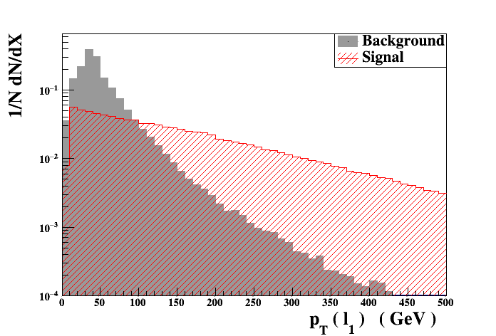
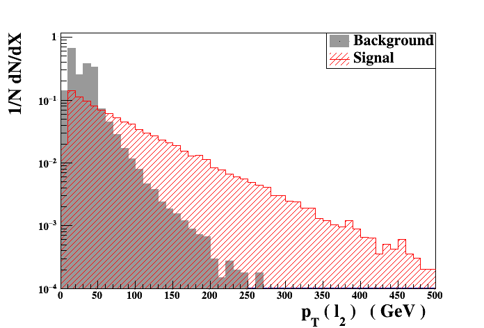
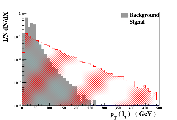
Figure 1: Normalized $p_{T}$ distributions for the leading (upper panels) and subleading (lower panels) leptons. The left and right panels refer to BP1 and BP2 respectively.

To understand the transverse momentum distribution of the leading lepton (the upper panels of Fig. 1), recall the decay chain for the signal processes. In all of the three processes, the heavy $W_{h}^{\pm}$ is produced, either directly or from the decay of heavy $T$-odd quarks. As already mentioned, for the parameter space of interest, the $W_{h}^{\pm}$ decay to $W^{\pm}+A_{h}$ with almost 100% branching ratio and, hence, the subsequent decay of the $W^{\pm}$ generates leptons in the final state. With the mass difference between the $W_{h}^{\pm}$ and SM $W^{\pm}$ bosons being so large, the latter would, typically, have a large $p_{T}$, even if the former had a small $p_{T}$. This translates to a large $p_{T}$ for the charged lepton emanating from the $W^{\pm}$ decay. Thus, for most events resulting from the process of (11b), the leading lepton tends to have a large $p_{T}$. For the other two production channels, at least a large fraction of the events would have the $Q_{h}$ decaying into $W_{h}^{\pm}$, thereby bestowing the latter with a large $p_{T}$ to start with. It should be realized though, that in each case, the possibility exists that, in a decay, the $p_{T}$ of a daughter, as defined in mother’s rest frame, is aligned against the mother’s $p_{T}$. While this degradation of the $p_{T}$ is not very important for the leading lepton, it certainly is so for the next-to-leading one, as is attested to by the lower panels of Fig. 1. It is instructive to examine the corresponding distributions for the background events. Since the $W$’s (or $Z$’s) now have typically lower $p_{T}$, the Jacobian peak at $m_{W}/2$ ($m_{Z}/2$) is quite visible, and particularly so for the next-to-leading lepton. For the leading one, the peak, understandably, gets smeared on account of the inherent $p_{T}$ of the decaying boson. This effect, of course, is more pronounced for the signal events. The second, and more pronounced, peak in the lower panels of Fig. 1 result from non-resonant processes and/or configurations wherein the lepton travels against the direction of its parent. This motivates our cuts on the lepton $p_{T}$s.

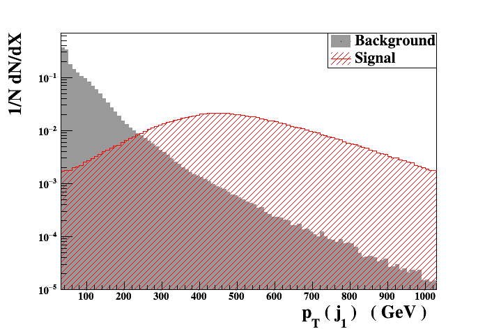
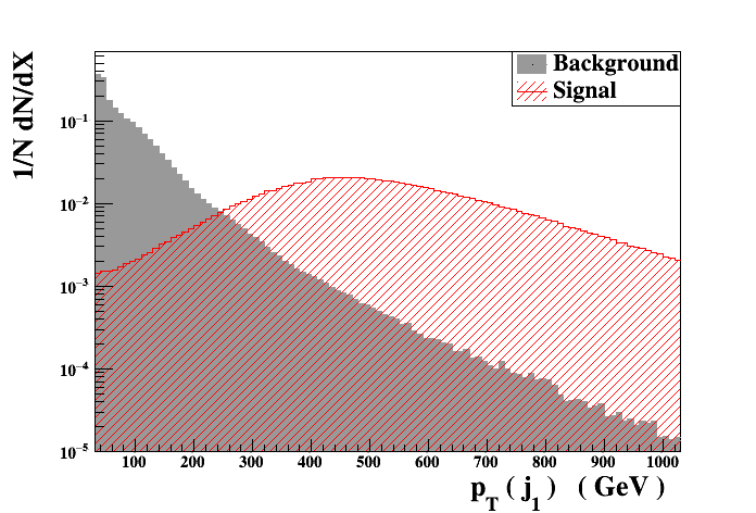
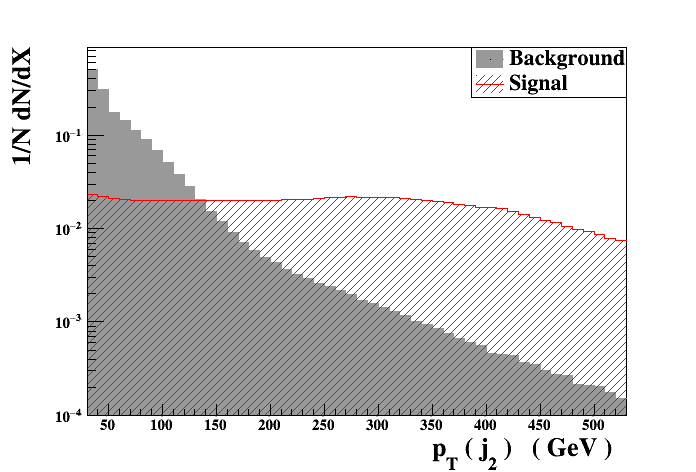
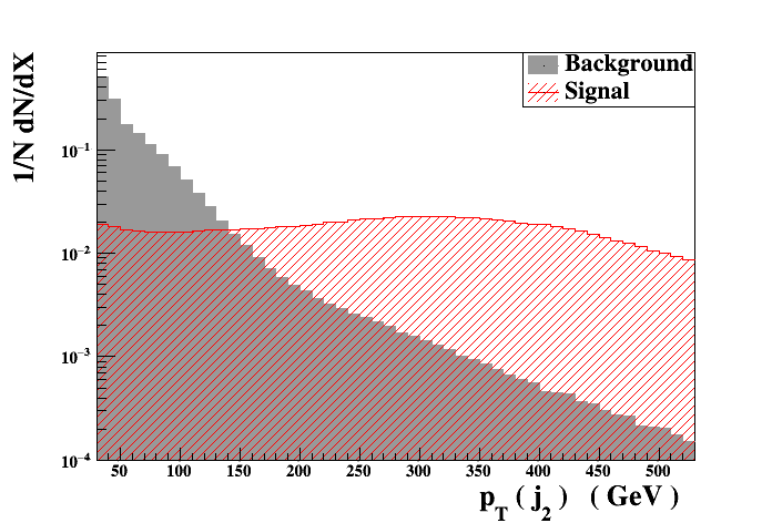
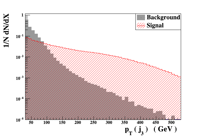
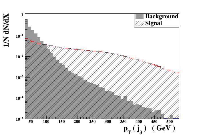
Figure 2: Normalized $p_{T}$ distributions for the three leading (top to bottom) non $b$-tagged jets for BP1 (left sets) and BP2 (right sets).

In an analogous fashion, the decay of the heavy $T$-odd quark (almost) always yields a high-$p_{T}$ jet owing to the large difference between its mass and those for $T$-odd bosons. Consequently, a requirement of $p_{T}(j_{1})\gtrsim 250$ GeV would eliminate only a very small fraction of the signal events (for each of the three channels, while, potentially, removing a significant fraction of the background events (see upper panels of Fig. 2). For process (11a), the decay of the second $Q_{h}$ would lead to a jet almost as hard. On the other hand, for channels (11b & 11c), the second jet results only from the decays of the $W^{\pm}$ or the $H$. Intrinsically much softer, these still gain from the $p_{T}$ of the mother. Consequently, the second leading jet, very often, may have a $p_{T}$ larger than 200 GeV (see the middle panels of Fig. 2). For the processes under discussion, a third jet can only result from the (cascade) decay of a SM boson, and, hence, is typically softer (the lower panels of Fig. 2) and hence, for three-jet final states, the requirement on the third jet $p_{T}$ should not be much stricter than about 45 GeV.

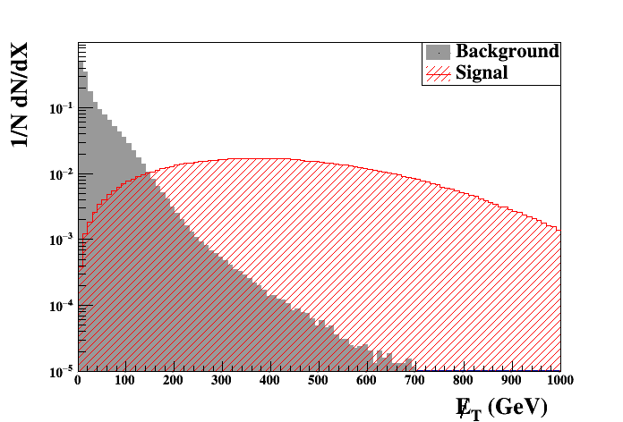
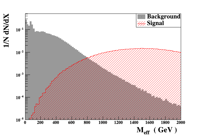
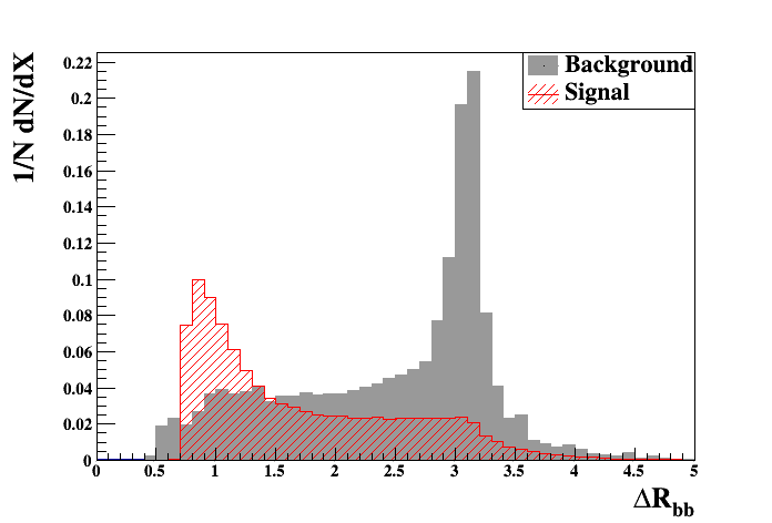
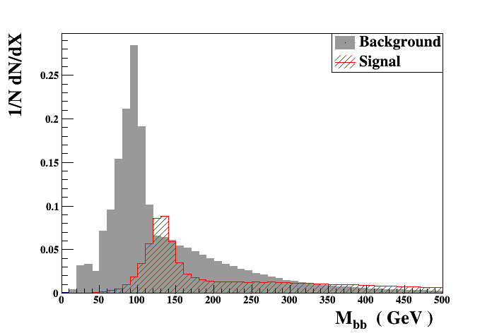
Figure 3: Normalized distributions for the missing transverse energy (top panels), the effective mass (second row), the $b\bar{b}$ invariant mass (third row) and ${\Delta R}_{\rm bb}$ (bottom panels). In each case, the left and right panels correspond to BP1 and BP2 respectively.

Next, we turn to some derived kinematic variables. The first quantity of interest is the missing transverse energy ($E_{T}/\;\>$). For the background events, this arises from the neutrinos (courtesy $W^{\pm}$ or $Z$ decays) or mismeasurement of the jet and lepton momenta. For the signal events, this receives an additional contribution from the heavy photon $A_{h}$, which is stable because of $T$-parity. Not only does the $A_{h}$ have a large mass, but also a large $p_{T}$ owing to the large difference in the masses of the mother and the daughters (on each occasion wherein it is produced). Consequently, the $E_{T}/\;\>$ spectrum is much harder for the signal (the upper panels of Fig. 3) and a requirement of $E_{T}/\;\>>250$ GeV would significantly improve the signal to background ratio.

Another variable of interest is the effective mass variable defined as

$$M_{\rm eff}=\sum_{n=1}^{4}|p_{T}(j)|_{n}+E_{T}/\;\>\,$$ (16)

where the sum goes over up to four jets. Similar to the case for the $E_{T}/\;\>$ distribution, the high masses of the exotic $T$-odd particles leads to a large $M_{\rm eff}$ for the signal events as one can see from the second panel of Fig. 3. Hence, a significant ($\rm M_{eff}$) cut also helps in reducing the background events.

Finally, for events with two tagged $b$-jets, we may consider the invariant mass of the pair (the third row of Fig. 3). In the signal events, the $Z_{h}$ decays to a Higgs boson and $A_{h}$, with the former decaying predominantly into a $b{\bar{b}}$ pair. Due to the large mass difference between $Z_{h}$ and $A_{h}$, the Higgs boson will be produced with a high $p_{T}$ which will be imparted to its decay products. As a result, the $b{\bar{b}}$ pair will be produced with a relatively small opening angle. On the other hand, the $b$’s in the SM background arise, primarily, from three classes of processes: ($a$) the decay of different top-quarks where the separation between them show a much broader structure; ($b$) the decay of a $Z$ boson, wherein the invariant mass would peak at $m_{Z}$, and owing to the relatively low momentum of the $Z$, the $b$’s be well-separated (in fact, close to being back-to-back); and ($c$) from non-resonant processes where the $b$’s would be softer and, again, $\Delta R_{b\bar{b}}$ would have a wider distribution. These features are well reflected by the third and fourth rows of Fig. 3. It is, thus, expected that a judicious upper cut on $\Delta R_{b\bar{b}}$ would definitely improve the signal significance. Similarly, a good energy-momentum resolution for the $b$-jets would serve to remove much of the $Z$-background.

3.1 Cut Analysis:

All the processes in Eq. (11) may contribute to a given final state—of Eq. (13)—and, henceforth, we include all under ‘Signal’, while ‘Background’ receives contributions from all SM processes leading to the particular final state.

In addition to the basic cuts of Eq. (14), further selection cuts may be imposed in order to improve the signal to background ratio. Understandably, these selections cuts would depend on the final state under consideration, both in respect of the differences in event topology for the signal and the background, as well as on the actual size of the signal. In particular, we are guided by the requirement that not too large an integrated luminosity is required to reach a $5\sigma$ significance ($S=5$), with $S$ being

$$S = \frac{N_{S}}{\sqrt{N_{S}+N_{B}}}\,\ ,$$ (17)

where $N_{S}$ and $N_{B}$ represent number of signal and background events respectively. We now take up each final state given in Eq. (13) and describe the kinematic cut flow followed in selecting events for the signal while suppressing the background.

3.1.1 $1\ell^{\pm}+nj+E_{T}/\;\>$ ; $n\geq 3$

This final state for the signal receives contribution from both the strongly produced $T$-odd quark pair as well as the associated production modes, thus giving us the maximum signal event rate amongst the final states under consideration. Here the single charged lepton almost always comes from the decay of a $W$ boson resulting from the cascades. The selection cuts, in the order that they are imposed, are:

1. $p_{T}(j_{3})>45$ GeV and $|\eta(j)|<2.5$ (C1–1): In other words, we demand that our final state has at least three jets within the given pseudo-rapidity range, each with a minimum $p_{T}$ of 45 GeV. This choice is motivated by the lowest panels of Fig. 2.

2. $p_{T}(j_{1})>250$ GeV (C1–2): Given that the hardest jet is, typically, much harder for the signal events than it is for the background (see top panels of Fig. 2), we ask that $p_{T}(j_{1})>250$ GeV. This, understandably, helps increase the signal to noise ratio to a remarkable extent.

3. $p_{T}(j_{2})>200$ GeV (C1–3): Similarly, we demand that the $p_{T}$ of the second hardest jet be more than 200 GeV. In particular, this reduces (moderately) the $t\bar{t}$ and $W+n$-jets background (with only a smaller effect on the $Z$ background) while having only a marginal effect on the signal strength.

4. $\rm M_{eff}>1.2$ TeV (C1–4): Motivated by the second row of Fig. 3, we demand that $M_{\rm eff}>1.2$ TeV. Such a high value effectively suppresses the background without reducing much of the signal.

5. $E_{T}/\;\>>250$ GeV (C1–5): The top row of Fig. 3 bears our (previously stated) expectations that the extent of transverse momentum imbalance ($E_{T}/\;\>$) would be far larger for the signal events than that for the background. Consequently, this requirement improves considerably the signal to background ratio.

6. $p_{T}(\ell_{1})>20$ GeV (C1–6): Finally, to distinguish this final state from that considered in Sec. 3.1.3, we require that there be only one isolated charged lepton $e,\mu$ with a $p_{T}$ more than 20 GeV.

		Effective Cross-section(fb) after the cut						${\cal L}_{5\sigma}$
SM-background	Production Cross-sec. (fb)	C1–1	C1–2	C1–3	C1–4	C1–5	C1–6
t $+$ jets	$2.22\times 10^{5}$	$6.12\times 10^{4}$	$3.34\times 10^{3}$	$1.84\times 10^{3}$	202	13.8	2.8
t$\bar{\rm t}+$ jets	$7.07\times 10^{5}$	$4.37\times 10^{5}$	$4.54\times 10^{4}$	$2.51\times 10^{4}$	$5.38\times 10^{3}$	453	123
W $+$ jets	$1.54\times 10^{8}$	$1.37\times 10^{6}$	$9.06\times 10^{4}$	$5.33\times 10^{4}$	$8.99\times 10^{3}$	679	39.9
Z $+$ jets	$4.54\times 10^{7}$	$8.49\times 10^{5}$	$4.12\times 10^{4}$	$2.65\times 10^{4}$	$3.75\times 10^{3}$	162	0
WW $+$ jets	$8.22\times 10^{4}$	$3.50\times 10^{4}$	$1.42\times 10^{3}$	800	51.2	5.1	1.5
ZZ $+$ jets	$1.10\times 10^{4}$	$1.91\times 10^{3}$	162	103	21.9	2.8	0.2
WZ $+$ jets	$3.81\times 10^{4}$	$8.30\times 10^{3}$	$1.39\times 10^{3}$	888	214	29.4	5.6
t$\bar{\rm t}+$W	351	238	45.8	24.9	5.9	0.8	0.2
t$\bar{\rm t}+$Z	585	435	101	55.3	15.6	1.8	0.3
t$\bar{\rm t}+$H	400	316	69.9	39.8	11.6	1.1	0.3
Total background							173.8
BP1	205	168	164	148	138	114	25.3	7.8 $\rm fb^{-1}$
BP2	153	129	126	115	109	91.8	15.2	20.4 $\rm fb^{-1}$

Table 3: Cut-flow for final state $(i)$ at $\sqrt{s}=13$ TeV. ${\cal L}_{5\sigma}$ is the integrated luminosity required to reach a $5\sigma$ significance.

		Effective Cross-section(fb) after the cut						${\cal L}_{5\sigma}$
SM-background	Production Cross-sec. (fb)	C1–1	C1–2	C1–3	C1–4	C1–5	C1–6
t $+$ jets	$2.49\times 10^{5}$	$6.86\times 10^{4}$	$3.74\times 10^{3}$	$2.06\times 10^{3}$	226	15.5	3.1
t$\bar{\rm t}+$ jets	$7.96\times 10^{5}$	$4.92\times 10^{5}$	$5.11\times 10^{4}$	$2.82\times 10^{4}$	$6.06\times 10^{3}$	509	138
W $+$ jets	$1.66\times 10^{8}$	$1.47\times 10^{6}$	$9.69\times 10^{4}$	$5.71\times 10^{4}$	$9.63\times 10^{3}$	728	42.8
Z $+$ jets	$4.86\times 10^{7}$	$9.10\times 10^{5}$	$4.42\times 10^{4}$	$2.84\times 10^{4}$	$4.03\times 10^{3}$	173	0
WW $+$ jets	$9.04\times 10^{4}$	$3.85\times 10^{4}$	$1.56\times 10^{3}$	879	56	5.6	1.7
ZZ $+$ jets	$1.18\times 10^{4}$	$2.04\times 10^{3}$	173	109	23.4	3.1	0.2
WZ $+$ jets	$4.21\times 10^{4}$	$9.18\times 10^{3}$	$1.54\times 10^{3}$	980	236	32	6.2
t$\bar{\rm t}+$W	398	270	52.0	28.3	6.7	0.9	0.3
t$\bar{\rm t}+$Z	706	526	122	66.8	18.8	2.2	0.4
t$\bar{\rm t}+$H	479	379	83.7	47.7	13.9	1.3	0.4
Total background							193.1
BP1	275	225	220	198	186	154	34.0	4.9 $\rm fb^{-1}$
BP2	208	174	170	156	148	124	20.7	12.5 $\rm fb^{-1}$

Table 4: Cut-flow for final state $(i)$ at $\sqrt{s}=14$ TeV.

In Tables 3(4), we display the effect, for $\sqrt{s}=13(14)$ TeV, that these cuts have on the signal and background events, when applied successively in the order described above. It is noteworthy that a discovery in this final state is possible at the current LHC Run with an integrated luminosity as little as $\sim 8~{}{\rm fb^{-1}}$ and $\sim 20~{}{\rm fb^{-1}}$ for BP1 and BP2 respectively. The corresponding numbers for LHC Run II are $\sim 5~{}{\rm fb^{-1}}$ and $\sim 12~{}{\rm fb^{-1}}$ respectively.

3.1.2 $1\ell^{\pm}+2b+j+E_{T}/\;\>$

Since the interest in this channel owes to the possibility of reconstructing the Higgs (and possibly develop an experimental handle on the very structure of the theory), the cuts now have to be reorganized keeping in mind both the origin (and, hence, the distributions) of the $b$-jets, as well as the signal strength.

1. $p_{T}(\ell_{1})>20$ GeV (C2–1): A single isolated lepton is required with a $p_{T}$ more than 20 GeV.

2. $|\eta(j_{1})|<2.5~{}\&~{}p_{T}(j_{1})>250$ GeV (C2–2): This is exactly akin to cut C1–2 of Sec. 3.1.1 and owes to the fact that the origin of the hardest jet is the same for the two configurations.

3. $E_{T}/\;\>>250$ GeV (C2–3): This, again, is similar to cut C1–5 of Sec. 3.1.1, and particularly helps eliminate much of the dominant $t\bar{t}$ background.

4. $p_{T}(b_{2})>40$ GeV (C2–4): As far as the signal events are concerned, the $b$-jets arise from the decay chain $Z_{h}\to A_{h}+H\to A_{h}+b\bar{b}$. The large mass difference between the $Z_{h}$ and $A_{h}$ would be manifested in a large boost for the $H$ which, very often, would be translated to a large $p_{T}$ for the $b$-jets. On the other hand, the SM background is dominated by the $t\bar{t}$ contribution, with typically, has a smaller $p_{T}$ for the $b$-jets. Thus, requiring that at least two $b$-jets have substantial $p_{T}$ would discriminate against the background. It might seem that imposing a harder cut on $p_{T}(b_{1})$ would be beneficial. While this, per se, is indeed true, such a gain is subsumed (and, in fact, bettered) by the next two cuts. Hence, we desist from imposing one such.

5. ${\Delta R}_{b\bar{b}}<1.5$ (C2–5): The aforementioned large boost for the $H$ in the signal events would, typically, result in the two $b$-jets being relatively close to each other. On the other hand, the background events from $t\bar{t}$ would have a much wider distribution, whereas $b$’s emanating from associated $H$-production (which, in the SM, is dominated by low-$p_{T}$ Higgs) would, preferentially, be back to back (see third row of Fig. 3). Thus, an upper limit on the angular separation between the two tagged $b$-jets considerably improves the signal-to background ratio.

6. Additional cut $110<M_{b\bar{b}}<160$ GeV (C2–6): This, obviously, serves to accentuate the contribution from an on-shell Higgs.

		Effective Cross-section(fb) after the cut					${\cal L}_{5\sigma}$
SM-background	Production Cross-section (fb)	C2–1	C2–2	C2–3	C2–4	C2–5
t $+$ jets	$2.22\times 10^{5}$	$3.64\times 10^{4}$	685	54.7	2.7	0.56
t$\bar{\rm t}+$ jets	$7.07\times 10^{5}$	$1.93\times 10^{5}$	$1.05\times 10^{4}$	826	113	16.8
W $+$ jets	$1.54\times 10^{8}$	$1.53\times 10^{7}$	$1.73\times 10^{4}$	$1.99\times 10^{3}$	0	0
Z $+$ jets	$4.54\times 10^{7}$	$2.12\times 10^{6}$	$4.12\times 10^{3}$	89.9	0	0
WW $+$ jets	$8.22\times 10^{4}$	$2.21\times 10^{4}$	438	41.6	0.45	0
ZZ $+$ jets	$1.10\times 10^{4}$	$1.22\times 10^{3}$	27.8	1.8	0	0
WZ $+$ jets	$3.81\times 10^{4}$	$6.73\times 10^{3}$	398	54.7	0.18	0.09
t$\bar{\rm t}+$W	351	131	13.5	1.8	0.16	0.02
t$\bar{\rm t}+$Z	585	189	24.6	2.8	0.3	0.06
t$\bar{\rm t}+$H	400	128	14.5	1.3	0.2	0.05
Total background						17.5
BP1	205	64.8	58.4	46.4	2.3	1.5	211.1 $\rm fb^{-1}$
BP2	153	38.1	34.3	27.7	1.2	0.82	681.1 $\rm fb^{-1}$

	Effective Cross-section(fb) after additional cut (C2–6)	${\cal L}_{5\sigma}$
Total SM background	4.8
BP1	0.86	191.3 $\rm fb^{-1}$
BP2	0.49	551 $\rm fb^{-1}$

Table 5: Cut-flow for final state $(ii)$ at $\sqrt{s}=13$ TeV.

		Effective Cross-section(fb) after the cut					${\cal L}_{5\sigma}$
SM-background	Production Cross-sec. (fb)	C2–1	C2–2	C2–3	C2–4	C2–5
t $+$ jets	$2.49\times 10^{5}$	$4.09\times 10^{4}$	769	61.4	3.0	0.63
t$\bar{\rm t}+$ jets	$7.96\times 10^{5}$	$2.18\times 10^{5}$	$1.18\times 10^{4}$	929	127	18.9
W $+$ jets	$1.66\times 10^{8}$	$1.64\times 10^{7}$	$1.85\times 10^{4}$	$2.14\times 10^{3}$	0	0
Z $+$ jets	$4.86\times 10^{7}$	$2.27\times 10^{6}$	$4.42\times 10^{3}$	96.4	0	0
WW $+$ jets	$9.04\times 10^{4}$	$2.43\times 10^{4}$	481	45.8	0.50	0
ZZ $+$ jets	$1.18\times 10^{4}$	$1.31\times 10^{3}$	29.7	1.9	0	0
WZ $+$ jets	$4.21\times 10^{4}$	$7.44\times 10^{3}$	439	60.5	0.20	0.12
t$\bar{\rm t}+$W	398	149	15.3	2.1	0.2	0.03
t$\bar{\rm t}+$Z	706	228	29.8	3.4	0.4	0.07
t$\bar{\rm t}+$H	479	154	17.4	1.6	0.3	0.06
Total background						19.7
BP1	275	86.2	77.7	61.8	3.2	2.0	135.6 $\rm fb^{-1}$
BP2	208	51.6	46.3	37.5	1.7	1.2	362.8 $\rm fb^{-1}$

	Effective Cross-sec. (fb) after additional cut (C2–6)	${\cal L}_{5\sigma}$
Total SM background	5.4
BP1	1.2	123.8 $\rm fb^{-1}$
BP2	0.7	319.8 $\rm fb^{-1}$

Table 6: Cut-flow for final state $(ii)$ at $\sqrt{s}=14$ TeV.

The effects of the aforementioned cuts are summarised in Tables 5(6). As expected, the signal strength is much weaker when compared to that discussed in Sec. 3.1.1. While the background rate suffers a suppression too, it is not enough and the required integrated luminosity is much larger in the present case. However, the combination of cuts on $\Delta R_{b\bar{b}}$ and $M_{b\bar{b}}$ brings discovery into the realm of possibility even for the present run of the LHC and certainly so for that at $\sqrt{s}=14$ TeV.

3.1.3 $2\ell^{\pm}+nj+E_{T}/\;\>$ ; $n\geq 2$

This final state receives contributions only from the primary production channels of Eq. (11a & 11b), and not from that of Eq. (11c). Consequently, the signal size is smaller. However, the higher multiplicity of the charged lepton in the final state proves helpful in suppressing the background, provided we re-tune the kinematic selections as follows:

1. $|\eta_{j}|<2.5$ (C3–1): The requirement of jet “centrality” remains the same.

2. $p_{T}(j_{1})>300~{}\rm GeV$ (C3–2): The requirement on the hardest jet is now strengthened. This reduces the cross-sections for most of the background subprocesses by 2-3 order of magnitude whereas the signal cross-section is reduced only by a few percent.

3. $p_{T}(j_{2})>200~{}\rm GeV$ (C3–3): The preceding cut (C3–2) also serves to harden the spectrum of the next sub-leading jet. Although this happens for both signal and background, the effect is larger for the former. This allows us to demand that the next to leading jet should have a minimum $p_{T}$ of 200 GeV. While the improvement is not as dramatic as in the case of C3–2, the signal to noise ratio does improve fairly (see Table. 7(8)).

4. $p_{T}(\ell_{1})>20~{}\rm GeV$ (C3–4): As in the previous cases, this requirement on the hardest isolated lepton is a very good discriminant. Most of the major background sources are suppressed by at least an order of magnitude (see Table. 7(8)), with the suppressions for the single-top and $Z+n$-jets production being even more pronounced.

5. $p_{T}(\ell_{2})>20~{}\rm GeV$ (C3–5): The success of C3–4 prompts us to require that even the next hardest isolated lepton should have $p_{T}>20$ GeV. As Table. 7(8) testifies, the major backgrounds (after the imposition of C3–4), namely $t\bar{t}$– and $W+n$-jets production suffer severe suppression.

6. $\rm M_{eff}>1.2$ TeV (C3–6): Analogous to (C1–4), we impose a high value of $\rm M_{eff}$ to further suppress the background cross section.

7. $E_{T}/\;\>>250$ GeV (C3–7): Additionally, we demand a large $E_{T}/\;\>$ to enhance the signal significance.

		Effective Cross-section(fb) after the cut							${\cal L}_{5\sigma}$
SM-background	Production Cross-sec. (fb)	C3–1	C3–2	C3–3	C3–4	C3–5	C3–6	C3–7
t $+$ jets	$2.22\times 10^{5}$	$1.43\times 10^{5}$	$2.54\times 10^{3}$	$1.75\times 10^{3}$	104	0	0	0
t$\bar{\rm t}+$ jets	$7.07\times 10^{5}$	$6.09\times 10^{5}$	$3.21\times 10^{4}$	$2.11\times 10^{4}$	$2.82\times 10^{3}$	99	22.8	4.2
W $+$ jets	$1.54\times 10^{8}$	$4.43\times 10^{7}$	$7.47\times 10^{4}$	$5.47\times 10^{4}$	$3.48\times 10^{3}$	0	0	0
Z $+$ jets	$4.54\times 10^{7}$	$1.31\times 10^{7}$	$3.52\times 10^{4}$	$2.73\times 10^{4}$	737	270	18.0	0
WW $+$ jets	$8.22\times 10^{4}$	$6.44\times 10^{4}$	$1.13\times 10^{3}$	751	59	1.3	0.11	0.11
ZZ $+$ jets	$1.10\times 10^{4}$	$6.31\times 10^{3}$	154	111	6.5	2.9	0.60	0.04
WZ $+$ jets	$3.81\times 10^{4}$	$2.21\times 10^{4}$	$1.28\times 10^{3}$	907	101	14.4	3.2	0.55
t$\bar{\rm t}+$W	351	308	35.4	22.3	4.5	0.1	0.05	0.03
t$\bar{\rm t}+$Z	585	532	76.9	48.4	8.3	0.9	0.17	0.06
t$\bar{\rm t}+$H	400	369	50.1	33.1	6.0	0.4	0.18	0.08
Total background								5.1
BP1	205	198	186	163	42.8	3.1	2.4	2.1	40.8 $\rm fb^{-1}$
BP2	153	149	141	126	25	1.3	0.96	0.84	210.4 $\rm fb^{-1}$

Table 7: Cut-flow for final state $(iii)$ at $\sqrt{s}=13$ TeV.

		Effective Cross-section(fb) after the cut							${\cal L}_{5\sigma}$
SM-background	Production Cross-sec. (fb)	C3–1	C3–2	C3–3	C3–4	C3–5	C3–6	C3–7
t $+$ jets	$2.49\times 10^{5}$	$1.60\times 10^{5}$	$2.85\times 10^{3}$	$1.96\times 10^{3}$	116	0	0	0
t$\bar{\rm t}+$ jets	$7.96\times 10^{5}$	$6.86\times 10^{5}$	$3.62\times 10^{4}$	$2.37\times 10^{4}$	$3.17\times 10^{3}$	111	25.7	4.7
W $+$ jets	$1.66\times 10^{8}$	$4.75\times 10^{7}$	$8.00\times 10^{4}$	$5.86\times 10^{4}$	$3.72\times 10^{3}$	0	0	0
Z $+$ jets	$4.86\times 10^{7}$	$1.40\times 10^{7}$	$3.77\times 10^{4}$	$2.93\times 10^{4}$	790	289	19.3	0
WW $+$ jets	$9.04\times 10^{4}$	$7.08\times 10^{4}$	$1.24\times 10^{3}$	826	64.9	1.4	0.13	0.13
ZZ $+$ jets	$1.18\times 10^{4}$	$6.74\times 10^{3}$	164	118	6.9	3.1	0.64	0.04
WZ $+$ jets	$4.21\times 10^{4}$	$2.45\times 10^{4}$	$1.41\times 10^{3}$	$1.02\times 10^{3}$	112	15.9	3.5	0.61
t$\bar{\rm t}+$W	398	349	40.1	25.3	5.1	0.2	0.06	0.04
t$\bar{\rm t}+$Z	706	642	92.9	58.4	10.0	1.1	0.21	0.07
t$\bar{\rm t}+$H	479	443	60	39.7	7.2	0.5	0.22	0.1
Total background								5.7
BP1	275	266	249	219	57.2	4.3	3.2	2.8	27.1 $\rm fb^{-1}$
BP2	208	201	190	171	34.5	1.9	1.4	1.2	119.8 $\rm fb^{-1}$

Table 8: Cut-flow for final state $(iii)$ at $\sqrt{s}=14$ TeV.

Note that although the dilepton final state has a reduced signal cross-section as compared to that with a single lepton, the requirement of a second isolated lepton also significantly reduces the background. Therefore, this final state requires moderate values for integrated luminosity at 13(14) TeV LHC, namely around $\sim 40(26)$ and $\sim 203(116)~{}\rm fb^{-1}$ for BP1 and BP2 respectively, which would be accessible in the current run of LHC.

At this point, we would like to mention that the benchmark points considered in our analysis can also be probed via the pair production of heavy $T$-odd gauge bosons ($W_{H}/Z_{H}$). However, the later processes being purely electroweak in nature yields much lower cross-section which in turn require significantly higher luminosity to reach the same signal significance as ours. This has been studied in Ref. [29].

4 Summary and conclusions

The very lightness of the Higgs boson that was discovered at the LHC has been a cause for concern, especially in the absence of any indication for physics beyond the SM that could be responsible for keeping it light. Amongst others, Little Higgs scenarios provide an intriguing explanation for the same. While several variants have been considered in the literature, in this paper, we examine a particularly elegant version, namely the Littlest Higgs model with a $Z_{2}$ symmetry ($T$-parity). The latter not only alleviates the severe constraints (on such models) from the electroweak precision measurements but also provides for a viable Dark Matter candidate in the shape of $A_{h}$, the exotic gauge partner of the photon.

At the LHC, the exotic particles can only be pair-produced on account of the aforementioned $T$-parity. Understandably, the production cross sections are, typically, the largest for the strongly-interacting particles. For example, if the exotic quarks $Q_{ih}$ are light enough to have a large branching fraction into their SM counterparts and the $A_{h}$, we would have a very pronounced excess in a final state comprising a dijet along with large missing-$p_{T}$ [30]. On the other hand, if the $Q_{ih}$ are heavier than $W_{h}$ and $Z_{h}$ (as can happen for a wide expanse of the parameter space) then they decay into the latter instead, with these, in turn decaying into their SM counterparts (or the Higgs), resulting in a final state comprising multiple jets, possibly leptons and missing-$p_{T}$ [39, 40], and it is this possibility that we concentrate on. The parameter space of interest is the two-dimensional one, spanned by $f$, the scale of breaking of the larger symmetry and $\kappa$, the universal Yukawa coupling. Although a part of it is already ruled out by the negative results from the 8 TeV run, a very large expanse is still unconstrained by these analyses. We illustrate our search strategies choosing representative benchmark points from within the latter set. We consider not only the production of a pair of exotic quarks, but also the associated production of $W_{h}/Z_{h}$ with such a quark. Concentrating on the final state comprising leptons plus jets plus missing transverse energy, we consider all the SM processes that could conspire to contribute as background to our LHT signal, and perform a full detector level simulation of the signal and background to estimate the discovery potential at the current run and subsequent upgrade of the LHC.

The large mass difference between the $Q_{ih}$ and $W_{h}/Z_{h}$ results in large momenta for at least a few of the jets. Similarly, the even larger mass difference between the $W_{h}/Z_{h}$ and the $A_{h}$ results, typically, in large missing-momentum. This encourages us to consider final states consisting of hard jets and leptons and large missing transverse momentum. We observe that final states with only one isolated charged lepton ($e^{\pm},\mu^{\pm}$) and with at least three jets and substantial missing transverse energy are the ones most amenable to discovery. For example, at the 13(14) TeV LHC with only $8(5)~{}\rm fb^{-1}$ and $20(12)~{}\rm fb^{-1}$ integrated luminosity for our BP1 and BP2 respectively. A confirmatory test is afforded by a final state requiring one extra isolated lepton. Though this decreases the signal cross-section significantly, LHC Run II can still reach the discovery level, but now only with $40(26)~{}\rm fb^{-1}$ and $203(116)~{}\rm fb^{-1}$ integrated luminosity at 13(14) TeV.

We however wish to highlight, through this work, a more interesting signal, one with 2 tagged $b$-jets in the final state. As discussed earlier (Eq. (12c)), the heavy $Z_{h}$ boson decays to a Higgs boson and the $A_{h}$ with almost 100% branching ratio. This presents us with an unique opportunity to reconstruct the Higgs mass from the tagged b-jets, thus providing us with an important insight into the LHT parameter space. As we have found out, the reconstruction of Higgs mass requires higher integrated luminosity (few hundred $\rm fb^{-1})$) but it is still within the reach of the LHC run II. We, thus, hope that our analysis demonstrates the viability of testing the LHT model in the current run of the LHC.

Acknowledgments: The work of S.K.R. was partially supported by funding available from the Department of Atomic Energy, Government of India, for the Regional Centre for Accelerator-based Particle Physics (RECAPP), Harish-Chandra Research Institute. D.C. acknowledges partial support from the European Union FP7 ITN INVISIBLES (Marie Curie Actions, PITN–GA–2011–289442), and the Research and Development grant of the University of Delhi. D.K.G and I.S would like to acknowledge the hospitality of RECAPP (HRI) in various occasions during the work. I.S would like to thank Juhi Dutta, Sujoy Poddar and Subhadeep Mondal for useful discussions and technical help. Computational work for this study was partially carried out at the cluster computing facility in the RECAPP.

References

- [1] ATLAS Collaboration, G. Aad et. al., Observation of a new particle in the search for the Standard Model Higgs boson with the ATLAS detector at the LHC, Phys.Lett. B716 (2012) 1–29, [arXiv:1207.7214].
- [2] CMS Collaboration, S. Chatrchyan et. al., Observation of a new boson at a mass of 125 GeV with the CMS experiment at the LHC, Phys.Lett. B716 (2012) 30–61, [arXiv:1207.7235].
- [3] N. Arkani-Hamed, A. G. Cohen, and H. Georgi, Electroweak symmetry breaking from dimensional deconstruction, Phys. Lett. B513 (2001) 232–240, [hep-ph/0105239].
- [4] N. Arkani-Hamed, A. G. Cohen, T. Gregoire, and J. G. Wacker, Phenomenology of electroweak symmetry breaking from theory space, JHEP 08 (2002) 020, [hep-ph/0202089].
- [5] N. Arkani-Hamed, A. G. Cohen, E. Katz, A. E. Nelson, T. Gregoire, and J. G. Wacker, The Minimal moose for a little Higgs, JHEP 08 (2002) 021, [hep-ph/0206020].
- [6] N. Arkani-Hamed, A. G. Cohen, E. Katz, and A. E. Nelson, The Littlest Higgs, JHEP 07 (2002) 034, [hep-ph/0206021].
- [7] M. Schmaltz, Physics beyond the standard model (theory): Introducing the little Higgs, Nucl. Phys. Proc. Suppl. 117 (2003) 40–49, [hep-ph/0210415]. [,40(2002)].
- [8] C. Csaki, J. Hubisz, G. D. Kribs, P. Meade, and J. Terning, Big corrections from a little Higgs, Phys. Rev. D67 (2003) 115002, [hep-ph/0211124].
- [9] J. L. Hewett, F. J. Petriello, and T. G. Rizzo, Constraining the littlest Higgs, JHEP 10 (2003) 062, [hep-ph/0211218].
- [10] C. Csaki, J. Hubisz, G. D. Kribs, P. Meade, and J. Terning, Variations of little Higgs models and their electroweak constraints, Phys. Rev. D68 (2003) 035009, [hep-ph/0303236].
- [11] M.-C. Chen and S. Dawson, One loop radiative corrections to the rho parameter in the littlest Higgs model, Phys. Rev. D70 (2004) 015003, [hep-ph/0311032].
- [12] W. Kilian and J. Reuter, The Low-energy structure of little Higgs models, Phys. Rev. D70 (2004) 015004, [hep-ph/0311095].
- [13] Z. Han and W. Skiba, Effective theory analysis of precision electroweak data, Phys. Rev. D71 (2005) 075009, [hep-ph/0412166].
- [14] G. Marandella, C. Schappacher, and A. Strumia, Little-Higgs corrections to precision data after LEP2, Phys. Rev. D72 (2005) 035014, [hep-ph/0502096].
- [15] Particle Data Group Collaboration, K. A. Olive et. al., Review of Particle Physics, Chin. Phys. C38 (2014) 090001.
- [16] H.-C. Cheng and I. Low, TeV symmetry and the little hierarchy problem, JHEP 09 (2003) 051, [hep-ph/0308199].
- [17] H.-C. Cheng and I. Low, Little hierarchy, little Higgses, and a little symmetry, JHEP 08 (2004) 061, [hep-ph/0405243].
- [18] I. Low, T parity and the littlest Higgs, JHEP 10 (2004) 067, [hep-ph/0409025].
- [19] J. Hubisz and P. Meade, Phenomenology of the littlest Higgs with T-parity, Phys. Rev. D71 (2005) 035016, [hep-ph/0411264].
- [20] J. Hubisz, P. Meade, A. Noble, and M. Perelstein, Electroweak precision constraints on the littlest Higgs model with T parity, JHEP 01 (2006) 135, [hep-ph/0506042].
- [21] A. Birkedal, A. Noble, M. Perelstein, and A. Spray, Little Higgs dark matter, Phys. Rev. D74 (2006) 035002, [hep-ph/0603077].
- [22] M. Asano, S. Matsumoto, N. Okada, and Y. Okada, Cosmic positron signature from dark matter in the littlest Higgs model with T-parity, Phys. Rev. D75 (2007) 063506, [hep-ph/0602157].
- [23] C.-R. Chen, M.-C. Lee, and H.-C. Tsai, Implications of the Little Higgs Dark Matter and T-odd Fermions, JHEP 06 (2014) 074, [arXiv:1402.6815].
- [24] J. Reuter, M. Tonini, and M. de Vries, Littlest Higgs with T-parity: Status and Prospects, JHEP 1402 (2014) 053, [arXiv:1310.2918].
- [25] Q.-H. Cao and C.-R. Chen, Signatures of extra gauge bosons in the littlest Higgs model with T-parity at future colliders, Phys. Rev. D76 (2007) 075007, [arXiv:0707.0877].
- [26] D. Song-Ming, G. Lei, L. Wen, M. Wen-Gan, and Z. Ren-You, -pair Production in the Littlest Higgs Model with T parity in NLO QCD at LHC, Phys. Rev. D86 (2012) 054027, [arXiv:1208.5532].
- [27] L. Wen, Z. Ren-You, G. Lei, M. Wen-Gan, and C. Liang-Wen, Precise QCD predictions on production in the Littlest Higgs Model with T parity at LHC, Phys. Rev. D87 (2013), no. 3 034034, [arXiv:1302.0052].
- [28] L.-W. Chen, R.-Y. Zhang, W.-G. Ma, W.-H. Li, P.-F. Duan, and L. Guo, Probing the littlest Higgs model with T parity using di-Higgs events through -pair production at the LHC in NLO QCD, Phys. Rev. D90 (2014), no. 5 054020, [arXiv:1409.1338].
- [29] Q.-H. Cao, C.-R. Chen, and Y. Liu, Testing LHT at the LHC Run-II, arXiv:1512.0914.
- [30] D. Choudhury, D. K. Ghosh, and S. K. Rai, Dijet Signals of the Little Higgs Model with T-Parity, JHEP 07 (2012) 013, [arXiv:1202.4213].
- [31] C. Han, A. Kobakhidze, N. Liu, L. Wu, and B. Yang, Constraining Top partner and Naturalness at the LHC and TLEP, Nucl. Phys. B890 (2014) 388–399, [arXiv:1405.1498].
- [32] N. Liu, L. Wu, B. Yang, and M. Zhang, Single top partner production in the Higgs to diphoton channel in the Littlest Higgs Model with -parity, Phys. Lett. B753 (2016) 664–669, [arXiv:1508.0711].
- [33] J. Alwall, R. Frederix, S. Frixione, V. Hirschi, F. Maltoni, et. al., The automated computation of tree-level and next-to-leading order differential cross sections, and their matching to parton shower simulations, JHEP 1407 (2014) 079, [arXiv:1405.0301].
- [34] A. Alloul, N. D. Christensen, C. Degrande, C. Duhr, and B. Fuks, FeynRules 2.0 - A complete toolbox for tree-level phenomenology, Comput.Phys.Commun. 185 (2014) 2250–2300, [arXiv:1310.1921].
- [35] T. Sjostrand, S. Mrenna, and P. Z. Skands, PYTHIA 6.4 Physics and Manual, JHEP 0605 (2006) 026, [hep-ph/0603175].
- [36] DELPHES 3 Collaboration, J. de Favereau et. al., DELPHES 3, A modular framework for fast simulation of a generic collider experiment, JHEP 1402 (2014) 057, [arXiv:1307.6346].
- [37] E. Conte, B. Fuks, and G. Serret, MadAnalysis 5, A User-Friendly Framework for Collider Phenomenology, Comput.Phys.Commun. 184 (2013) 222–256, [arXiv:1206.1599].
- [38] Calibration of the performance of -tagging for and light-flavour jets in the 2012 ATLAS data, Tech. Rep. ATLAS-CONF-2014-046, CERN, Geneva, Jul, 2014.
- [39] D. Choudhury and D. K. Ghosh, LHC signals of T-odd heavy quarks in the Littlest Higgs model, JHEP 08 (2007) 084, [hep-ph/0612299].
- [40] G. Cacciapaglia, S. R. Choudhury, A. Deandrea, N. Gaur, and M. Klasen, Dileptonic signatures of T-odd quarks at the LHC, JHEP 03 (2010) 059, [arXiv:0911.4630].