Zero-energy modes and valley asymmetry in the Hofstadter spectrum of bilayer graphene van der Waals heterostructures with hBN

Abstract

We investigate the magnetic minibands of a heterostructure consisting of bilayer graphene (BLG) and hexagonal boron nitride (hBN) by numerically diagonalizing a two-band Hamiltonian that describes electrons in BLG in the presence of a moiré potential. Due to inversion-symmetry breaking characteristic for the moiré potential, the valley symmetry of the spectrum is broken, but despite this, the zero-energy Landau level in BLG survives, albeit with reduced degeneracy. In addition, we derive effective models for the low-energy features in the magnetic minibands and demonstrate the appearance of secondary Dirac points in the valence band, which we confirm by numerical simulations. Then, we analyze how single-particle gaps in the fractal energy spectrum produce a sequence of incompressible states observable under a variation of carrier density and magnetic field.

I Introduction

Long-period moiré patterns are characteristic of well-aligned graphene heterostructures with hBN. They offer an experimentally-viable route ponomarenko_nature_2013 ; dean_nature_2013 ; hunt_science_2013 to observe fractal magnetic miniband spectra generic for electrons in two-dimensional superlattices in strong magnetic fields brown_physrev_1964 ; zak_physrev_1964a ; zak_physrev_1964b . These fractal miniband spectra, also known as Hofstadter’s butterflies hofstadter_prb_1976 , reflect the fact that the translational symmetry of a lattice, suppressed by the presence of a magnetic vector potential in the electron’s Schrödinger equation, is restricted to magnetic field values $B_{p/q}=(p/q)\phi_{0}/S$ corresponding to a rational fraction $p/q$ of magnetic flux quantum $\phi_{0}=h/e$ per unit cell area $S$ of the lattice brown_physrev_1964 ; zak_physrev_1964a ; zak_physrev_1964b . The generic features of fractal magnetic miniband spectra have been observed ponomarenko_nature_2013 ; hunt_science_2013 ; Yu_NatPhys_2014 ; wang_science_2015 and modeled wallbank_prb_2013 ; chen_prb_2014 ; Yu_NatPhys_2014 ; diez_prl_2014 ; moon_prb_2014 ; chizhova_prb_2014 ; wallbank_adp_2015 ; slotman_prl_2015 in monolayer graphene heterostructures with hBN, where the properties of Dirac electrons at the conduction/valence band edge allow for a straightforward interpretation of experimental observations, and have also been studied in slightly misaligned pairs of graphene flakes bistritzer_prb_2011 ; Santos_PRL_2007 . Modeling of the fractal magnetic miniband spectra of a bilayer graphene/hBN heterostructure is much more limited moon_prb_2014 , even though one of the first observations of this phenomena was in this system dean_nature_2013 .

In this Article, we study fractal magnetic minibands in bilayer graphene (BLG) subject to a moiré superlattice perturbation due to an hBN underlay. The low-energy Hofstadter butterfly spectra of a BLG-hBN heterostructure is dominated by bands related to the degenerate “zero-energy” Landau level (LL) states $n=0$ and $n=1$ of unperturbed BLG mccann_prl_2006 . We use a symmetry-based approach to model the influence of hBN on electrons in BLG, and we show that the spectra in BLG-hBN is a superposition of two very different miniband spectra associated with electrons in opposite valleys (Brillouin zone corners) of BLG’s band structure: the miniband spectrum in one valley is only weakly broadened by the superlattice potential and incorporates one unperturbed $n=0$ LL, while the miniband spectrum in the other valley is widely broadened. This valley asymmetry arises from spatial inversion symmetry breaking produced by the fact that the moiré perturbation only directly affects one of the two BLG layers. Since the zero energy LL states reside on different layers in opposite valleys, in one valley they are strongly influenced by the moiré perturbation, but in the other valley they are not.

These qualitative features agree with the results of the tight-binding model of Moon and Koshino moon_prb_2014 . In addition, we characterize different types of moiré superlattice perturbations including the possibilities that the perturbation creates potential asymmetry between the carbon atoms in BLG or introduces a spatial modulation of the nearest-neighbor carbon-carbon hopping amplitude. Hence, we find that the Dirac point at the conduction-valence band edge can be either gapless or gapped, and that a secondary Dirac point can appear in the valence band of BLG-hBN. Our model Hamiltonian is presented in Section II and its numerical diagonalization in the presence of a magnetic field, including methodology, results and discussion, is described in Section III, where we also derive simple effective Hamiltonians to describe low-energy features in the magnetic minibands and, also, an effective Hamiltonian to describe the secondary Dirac point. In Section IV, we show how gaps in the fractal energy spectrum are manifest as observable incompressible states under a variation of carrier density and magnetic field.

II Moiré superlattice Hamiltonian

II.1 Four band model

To describe the sublattice ($A/B$) and bottom/top ($1/2$) layer composition of electron states in Bernal-stacked BLG on a hBN underlay, we write down their Hamiltonian mccann_prl_2006 as a $4\times 4$ matrix,

$$\hat{\bm{H}}_{\xi}\!\!=\!\!\left(\!\!\begin{array}[]{cc}v\hat{\bm{p}}\!\cdot\!\bm{\sigma}+\hat{\bm{M}}_{\xi}&\gamma_{1}(\xi\sigma_{1}\!-\!i\sigma_{2})/2\\ (\gamma_{1}(\xi\sigma_{1}\!-\!i\sigma_{2})/2)^{\dagger}&v\hat{\bm{p}}\!\cdot\!\bm{\sigma}\end{array}\!\!\right)$$ (3)

$$\hat{\bm{M}}_{\xi}=vbu_{0}f_{+}\!+\xi vb\sigma_{3}u_{3}f_{-}+\xi v\bm{\sigma}\!\cdot\!\left[\bm{l}_{z}\!\times\!\nabla\!\left(u_{1}f_{-}\right)\right]\!.$$

Here, we use the basis of Bloch functions $(\phi_{A_{1}},\phi_{B_{1}},\phi_{A_{2}},\phi_{B_{2}})$ for valley $K$ ($\xi=1$), $(\phi_{B_{1}},-\phi_{A_{1}},\phi_{B_{2}},-\phi_{A_{2}})$ for valley $K^{\prime}$ ($\xi=-1$), and the $2\times 2$ Pauli matrices $\sigma_{1,2,3}$ act in the space of sublattice components. The term $v\hat{\bm{p}}\!\cdot\!\bm{\sigma}$ on the diagonal takes into account the electrons’ Dirac spectrum in each layer where $v\simeq 10^{8}\,$cm s^-1 deacon_prb_2007 is the Dirac velocity, $\hat{\bm{p}}=-i\nabla+e\bm{A}$, $[\nabla\times\bm{A}]_{z}=-B$, $\bm{\sigma}=(\sigma_{x},\sigma_{y})$, and $\hbar=1$, while $\gamma_{1}\simeq 0.4\,$eV kuzmenko_prb_2009 is the inter-layer hopping between $A_{2}$ and $B_{1}$ sublattices.

The term $\hat{\bm{M}}_{\xi}$ in Eq. (3) accounts for the moiré superlattice perturbation produced by the hBN substrate wallbank_prb_2013 ; chen_prb_2014 , and is applied only to the layer of the bilayer which is closest to the hBN (layer ‘$1$’) mucha-kruczynski_prb_2013 . Within the term $\hat{\bm{M}}_{\xi}$, the functions $f_{\pm}=\!\sum_{m}\!(\pm 1)^{m+\frac{1}{2}}e^{i\bm{b}_{m}\cdot\bm{r}}$, with $m=0,1,...,5$, are written using the shortest non-zero Bragg vectors of the moiré superlattice $\bm{b}_{m}=\hat{\bm{R}}_{m\pi/3}[1-(1+\delta)^{-1}\hat{\bm{R}}_{\theta}](0,\tfrac{4\pi}{\sqrt{3}l})$, where $\hat{\bm{R}}_{\varphi}$ describes anti-clockwise rotation by angle $\varphi$, $\delta\approx 1.8\%$ takes into account the relative lattice mismatch between graphene and hBN xue_natmater_2011 , $\theta$ is the misalignment angle between the two hexagonal lattices and $l=2.46\,$Å  is the lattice constant of graphene. For $\theta\ll 1$, $b=|\bm{b}_{m}|\approx\tfrac{4\pi}{\sqrt{3}l}\sqrt{\delta^{2}+\theta^{2}}$ so that the energy scale $vb$ obtains its minimum value of $vb\approx 0.35\,$eV at $\theta=0$. The strength of the various terms included in $\hat{\bm{M}}_{\xi}$ are controlled by separate dimensionless parameters, $u_{i=0,3,1}$, which describe in turn an electrostatic potential which does not distinguish between the two carbon sublattices ($u_{0}$), a sublattice-asymmetric part of the potential ($u_{3}$), and a spatial modulation of the nearest-neighbor carbon-carbon hopping amplitude ($u_{1}$).

II.2 Two band model

One of the most interesting features of electrons in BLG at strong magnetic fields is the degeneracy of two orbital LLs, with $n=0$ and $n=1$, which appear at $\epsilon=0$, the edge between the valence and conduction band. The mixing of these degenerate LLs by the moiré superlattice potential determines the main features of the lower-energy part of the magnetic miniband spectrum, shown in Fig. 1 for several different choices of moiré perturbation parameters $u_{i}$. These low-energy electron states in BLG can be described mccann_prl_2006 using a simplified two-band Hamiltonian, which can be obtained from Eq. (3) by a Schrieffer-Wolf projection onto the basis of Bloch states residing on $A_{1}$ and $B_{2}$ sublattices. For a BLG-hBN heterostructure, such a projection results in mucha-kruczynski_prb_2013 ,

$$\bm{\tilde{H}}_{\xi}=-\xi\frac{v^{2}}{\gamma_{1}}\left(\begin{array}[]{cc}0&\left(\hat{\bm{\pi}}^{\dagger}\right)^{2}\\ \hat{\bm{\pi}}^{2}&0\end{array}\right)+\bm{\tilde{M}}_{\xi},$$ (6)

$$\bm{\tilde{M}}_{1}=\left(\begin{array}[]{cc}vbg_{+}(r)&\tfrac{bv^{2}}{\gamma_{1}}h_{+}^{*}(r)\hat{\bm{\pi}}^{\dagger}\\[3.00003pt] \tfrac{bv^{2}}{\gamma_{1}}\hat{\bm{\pi}}h_{+}(r)&\tfrac{v^{3}b}{\gamma_{1}^{2}}\hat{\bm{\pi}}g_{-}(r)\hat{\bm{\pi}}^{\dagger}\end{array}\right),$$ (9)

$$\bm{\tilde{M}}_{\text{-}1}=\left(\begin{array}[]{cc}\tfrac{v^{3}b}{\gamma_{1}^{2}}\hat{\bm{\pi}}^{\dagger}g_{-}(r)\hat{\bm{\pi}}&\tfrac{bv^{2}}{\gamma_{1}}\hat{\bm{\pi}}^{\dagger}h_{-}(r)\\[3.00003pt] \tfrac{bv^{2}}{\gamma_{1}}h_{-}^{*}(r)\hat{\bm{\pi}}&vbg_{+}(r)\end{array}\right),$$ (12)

$$g_{\pm}(r)=\sum_{m}e^{ib_{m}.r}(u_{0}\pm iu_{3}(-1)^{m}),$$

$$h_{\pm}(r)=\pm iu_{1}\sum_{m}(-1)^{m}e^{ib_{m}.r}\left(b_{m}^{x}\pm ib_{m}^{y}\right)/b.$$

Hamiltonian $\bm{\tilde{H}}_{\xi}$ is written in the basis of the Bloch states $(\phi_{A_{1}},\phi_{B_{2}})$ for the $K$ valley and $(\phi_{B_{2}},-\phi_{A_{1}})$ for the $K^{\prime}$ valley using $\hat{\bm{\pi}}=\hat{\bm{p}}_{x}+i\hat{\bm{p}}_{y}$, and $\bm{b}_{m}=(b^{x}_{m},b^{y}_{m})$

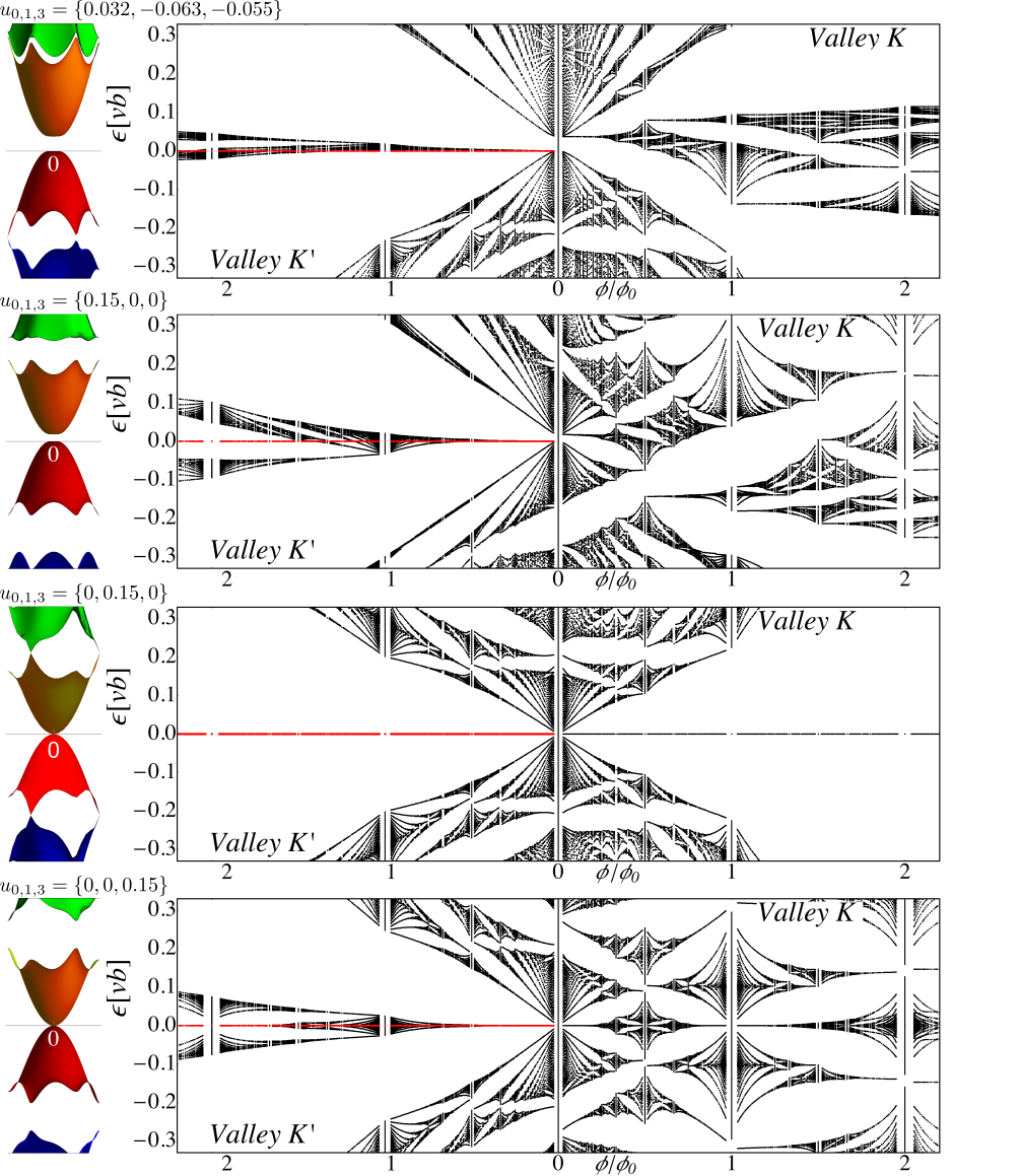
Figure 1: The $B=0$ minibands for the labeled superlattice perturbation parameters and $\theta=0$ (left panels), and the bandwidths of the magnetic minibands, shown separately for the $K^{\prime}$ and $K$ valleys, for the same superlattice parameters (central panels) A red line is used to indicate the unperturbed zero energy Landau level in the $K^{\prime}$-valley.

Examples of the zero magnetic field $K$-valley bandstructure of moiré perturbed BLG with $\theta=0$ are displayed in the left panels of Fig. 1. These spectra were calculated by numerical diagonalization of the Heisenberg matrix constructed from Hamiltonian (6) in a basis of unperturbed plane wave states. The corresponding dispersion in the $K^{\prime}$-valley is obtained using the relation, $\epsilon_{K^{\prime}}(\bm{k})=\epsilon_{K}(-\bm{k})$, which follows from the time-reversal symmetry of Hamiltonians (3) and (6) for $B=0$.

Each panel in Fig. 1 corresponds to a different set of moiré perturbation parameters $\{u_{0},u_{1},u_{3}\}$. The choice of parameters used in the top panel corresponds to the predictions of a pair of microscopic models, one based on hopping between graphene carbon atoms and hBN atoms, the other on scattering of graphene electrons by the quadropole electric moments of nitrogen atoms. Interestingly, these two models predict the same relative values for the moiré potential parameters wallbank_prb_2013 ,

$$u_{i=0,1,3}=V\left\{1/2,-\delta/\sqrt{\delta^{2}+\theta^{2}},-\sqrt{3}/2\right\},$$ (13)

where $V$ depends upon the specific microscopic parameters used to describe the hBN underlay. Here we take $V=0.063$, chosen to make the moiré perturbation strong enough that an almost gapless secondary Dirac point (sDP) is produced between the red and blue minibands in the valence band of the upper left panel of Fig. 1. Signatures of this feature were observed experimentally in Ref. dean_nature_2013 .

The other panels in Fig. 1 illustrate the influence of each $u_{i}$ parameter taken individually and they exemplify three additional scenarios: for $u_{0,1,3}=\{0.15,0,0\}$, the original Dirac point is gapped and there is no sDP (in the two valence bands closest to zero energy); for $u_{0,1,3}=\{0,0.15,0\}$, the original Dirac point and the sDP are both gapless (and there is a sDP in the conduction band); for $u_{0,1,3}=\{0,0,0.15\}$, the original Dirac point is gapless and there is no sDP.

III The BLG-hBN heterostructure in a magnetic field studied using the two band model

III.1 Methodology

Here we describe the numerical diagonalization of Hamiltonian (6) in the presence of a magnetic field. To simplify this calculation, we take account of the hexagonal symmetry of the moiré pattern and use a non-orthogonal coordinate system chen_prb_2014 $\bm{r}=(x_{1}\bm{a_{1}}+x_{2}\bm{a_{2}})/a$, where $\bm{a}_{1}=4\pi\bm{b}_{1}\times\bm{\hat{l}}_{z}/(\sqrt{3}b^{2})$ and $\bm{a}_{2}=4\pi\bm{\hat{l}}_{z}\times\bm{b}_{5}/(\sqrt{3}b^{2})$ are direct moiré lattice vectors and $a=|\bm{a}_{1}|$. In this basis the Landau gauge has the form $\bm{A}=Bx_{1}(\bm{a_{1}}-2\bm{a_{2}})/(\sqrt{3}a)$ which leads to

$$\hat{\bm{\pi}}=\tfrac{-2}{\sqrt{3}}\left[\partial_{x_{1}}\tau+(\partial_{x_{2}}-i\sqrt{3}eBx_{1}/2)\tau^{*}\right],$$

where $\tau=e^{i2\pi/3}$, and $e$ is the electron charge. For the wave-vector space, this determines $\bm{k}=k_{1}\bm{k}_{1}+k_{2}\bm{k}_{2}$ with $\bm{k}_{1}=2\bm{b}_{5}/(\sqrt{3}b)$ and $\bm{k}_{2}=2\bm{b}_{1}/(\sqrt{3}b)$. Hence, we employ the basis set of magnetic oscillator functions,

$$\varphi_{n}(k_{2})=\frac{\sqrt{3}e^{ik_{2}x_{2}}e^{-\frac{z^{2}}{2}-\frac{iz^{2}}{2\sqrt{3}}}}{\sqrt{n!2^{(n+1)}\lambda_{B}\sqrt{\pi}}}\mathbb{H}_{n}(\!z\!),$$ (14)

$$z=\frac{\sqrt{3}x_{1}}{2\lambda_{B}}-k_{2}\lambda_{B},\quad\lambda_{B}\!=\!1/\sqrt{|eB|},$$

$$\hat{\bm{\pi}}\varphi_{n}(k_{2})=-\tau\lambda_{B}^{-1}\sqrt{2n}\varphi_{n-1}(k_{2}),$$

where $\mathbb{H}_{n}(z)$ are the Hermite polynomials. For free electrons in BLG, the LL spectrum contains two degenerate states at $\epsilon=0$, and pairs of conduction/valence band states at $\epsilon_{n\geq 2}^{\alpha}=\alpha\sqrt{n(n-1)}/m\lambda_{B}^{2}$, $\alpha=\pm 1$,

$$\psi^{0}_{n=0,1}(k_{2})=\frac{1}{\sqrt{L}}\left(\begin{array}[]{c}\varphi_{n}(k_{2})\\ 0\end{array}\right)\,,$$ (17)

$$\psi_{|n|\geq 2}^{\alpha}(k_{2})=\frac{1}{\sqrt{2L}}\left(\begin{array}[]{c}\varphi_{n}(k_{2})\\ \text{-}\alpha\tau\varphi_{n\text{-}2}(k_{2})\end{array}\right)\,.$$ (20)

In general, the magnetic vector potential $\bm{A}(x_{1})$ breaks the symmetry of the Hamiltonian with respect to translations of the moiré superlattice. However, for magnetic flux $\phi=SB=\frac{p}{q}\phi_{0}$ where $p$ and $q$ are co-prime natural numbers and $S$ is the unit cell area of the moiré superlattice, translational symmetry is restored. Because of this, we consider a unit cell of the magnetic superlattice that is $q$ times larger than the unit cell of the moiré superlattice in both directions (hence its area is $q^{2}$ times larger) brown_physrev_1964 ; chen_prb_2014 . The magnetic translational group $G=\{\Theta_{\bm{X}}\equiv e^{ieBm_{1}qa\sqrt{3}x_{2}/2}T_{\bm{X}},\bm{X}=m_{1}q\bm{a}_{1}+m_{2}q\bm{a}_{2}\}$, where $T_{\bm{X}}$ describes geometrical translations and $m_{1}$ and $m_{2}$ are integers, commutes with Hamiltonian (6) and is isomorphic to the group of geometrical translation, so that its eigenstates form a plane wave basis $\Theta_{\bm{X}}|n^{\alpha}_{jt}(\bm{k})\rangle=e^{i\bm{k}\cdot\bm{X}}|n^{\alpha}_{jt}(\bm{k})\rangle$. Bloch functions $|n^{\alpha}_{jt}(\bm{k})\rangle$ exist in the magnetic Brillouin zone which is $q^{2}$ times smaller than that of the moiré superlattice brown_physrev_1964 and in which magnetic minibands are $q$-fold degenerate. For states with momentum $\bm{k}$ within this magnetic Brillouin zone,

$$|n^{\alpha}_{jt}(\bm{k})\rangle\!\!=\!\!\frac{1}{\sqrt{N}}\!\!\sum_{s=\text{-}N/2}^{N/2}\!\!\!e^{\text{-}ik_{1}qas}\psi_{n}^{\alpha}(k_{2}\!+\!\tfrac{\sqrt{3}}{2}b[ps\!+\!j\!+\!t\tfrac{p}{q}]),$$ (21)

where $N\rightarrow\infty$, and $j=0,\cdots,p-1$ indexes the magnetic sub-bands, and $t=0,\cdots,q-1$ indexes the above mentioned $q$-fold degeneracy Without loss of generality, we set $t=0$ and omit it, using the notation $|n^{\alpha}_{j}(\bm{k})\rangle$, from now on. In order to obtain the energy dispersion, we calculate the matrix elements of the perturbation, $\langle n^{\alpha}_{j}(\bm{k})|\bm{\tilde{H}}^{B}_{\xi}|\tilde{n}^{\tilde{\alpha}}_{\tilde{j}}(\tilde{\bm{k}})\rangle$, in this basis and diagonalize the resulting matrix chen_prb_2014 .

III.2 Results and discussion

The main panels of Fig. 1 show the magnetic spectrum of the BLG-hBN heterostructure for the four choices of moiré perturbation described above. For small flux, the magnetic miniband spectra can be traced to the sequence of Landau levels for moiré perturbed BLG. Near zero energy, the gap at the original Dirac point is seen in the magnetic spectra of the top two panels. The presence or absence of a secondary Dirac point (depending on the particular parameter set) is also clearly reflected in the magnetic spectra at small flux at the corresponding energy. At a higher flux, the Landau levels broaden and split, forming a fractal pattern, with the most striking features around zero energy.

For all parameter sets, the valley symmetry of the spectrum, preserved in the absence of a magnetic field, is lifted. This is because the moiré perturbation only affects the layer of BLG that is adjacent to the hBN and, thus, it breaks inversion symmetry. In conjunction with time-inversion symmetry breaking by a magnetic field, this allows the energy spectra for electrons in valleys $K$ and $K^{\prime}$ to be different moon_prb_2014 . In particular, note that, in the absence of the perturbation, the distribution of the wave function among the layers is, for a given Landau level, exactly inverted in the two valleys, Eqs. (17,20). The moiré potential affects only the wave function component in the layer adjacent to hBN, hence breaking the layer symmetry and leading to valley-asymmetric spectra with a gap.

Importantly, the spectrum in the valley for which the wave function sits on the layer further from the substrate contains a zero-energy Landau level completely decoupled from the rest of the spectrum (shown as a red line in the $K^{\prime}$-valley in Fig. 1). The spinor structure Eq. (17) of the two zero-energy states, $n=0,1$, for unperturbed electrons shows that the states in valley $K$ ($K^{\prime}$) are localized on the bottom (top) graphene layer only mccann_prl_2006 . Since the moiré perturbation does not directly influence the top layer, it does not couple the $n=0$ state in the $K^{\prime}$ valley to any other state and, thus, the $n=0$ state in this valley always persists. This coexistence of a zero-energy LL and a fractal spectrum of magnetic sub-bands creates a unique opportunity to observe the interplay between electron-electron interaction and Hofstadter’s quantization ghazaryan_prb_2015 ; wang_science_2015 .

Each of the panels in Fig. 1 display further features of interest. For the parameter set $u_{0,1,3}=\{0.032,-0.063,-0.055\}$ (upper panel), the $B=0$ miniband spectrum displays a slightly gapped sDP found in the first valence miniband, which produces a sequence of LL including tilted zeroth LLs, at the corresponding energy and weak magnetic fields ($\epsilon\approx-0.22\,vb$ $\phi/\phi_{0}\lesssim 0.2$). We shall discuss the sDP further in Section III.4 (a similar feature is present in the lower middle panel). For potential modulation taken in isolation, $u_{0,1,3}=\{0.15,0,0\}$, the band structure obeys six-fold rotation symmetry in each valley (left upper middle panel), in contrast to all other band structure images which only display symmetry under three-fold rotation. For the spatial modulation of the carbon-carbon hopping amplitude, $u_{0,1,3}=\{0,0.15,0\}$ (lower middle panels), the spectrum at both zero magnetic field and finite magnetic field obeys electron-hole symmetry, and the zeroth LL and first LL of the original Dirac point are completely degenerate in both valleys (discussed in Section III.3). For the sublattice-asymmetric potential, $u_{0,1,3}=\{0,0,0.15\}$ (lower panel), the bands at zero magnetic field are symmetric under the operation which combines electron-hole-reflection and a rotation by $\pi/3$, which is reflected in the electron-hole symmetry of the magnetic miniband widths in a magnetic field. Additionally for this perturbation, we find that the magnetic miniband structure around $\epsilon=0$ can form gapless linear or quadratic Dirac points, which produce sequences of LLs in the magnetic miniband spectrum, best visible around $\phi/\phi_{0}=2$ in the $K^{\prime}$-valley and $\phi/\phi_{0}=1$ in the $K$-valley (also see Section III.3).

III.3 Effective model of low energy features in the magnetic minibands

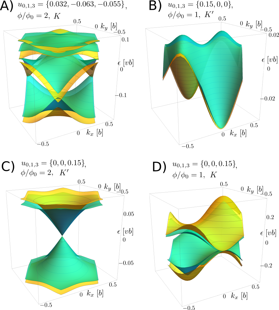
Figure 2: The full $(k_{x},k_{y})$-dispersion of magnetic minibands obtained by either diagonalizing effective Hamiltonians (22)-(29) (yellow), or the full numerical diagonalization of Hamiltonian (6) (turquoise).

The main features of the broadened magnetic miniband spectrum around zero energy at a simple fraction $\phi/\phi_{0}=1/q$ can be described by truncating the basis of Bloch functions Eq. (21) to the zeroth and first LL only, yielding effective Hamiltonians,

$$\bm{{\mathbb{H}}}_{K^{\prime}}=0\oplus vbD\omega(u_{0}f_{0}-u_{3}f_{1})\,,$$ (22)

$$\bm{{\mathbb{H}}}_{K}=vbDu_{0}\left(\begin{array}[]{cc}2f_{0}&\sqrt{2bl_{0}}f_{2}^{*}\\ \sqrt{2bl_{0}}f_{2}&(2-bl_{0})f_{0}\end{array}\right)$$ (25)

$$\qquad+vbDu_{3}\left(\begin{array}[]{cc}2f_{1}&\sqrt{2bl_{0}}f_{3}^{*}\\ \sqrt{2bl_{0}}f_{3}&(2-bl_{0})f_{1}\end{array}\right)\,,$$ (28)

$$f_{0}=c_{1}+c_{2}+(\text{-}1)^{q}c_{12},\ f_{1}=\text{-}s_{1}+s_{2}+(\text{-}1)^{q}s_{12}\,,$$

$$f_{2}=\tau^{*}\!s_{1}\!-\!s_{2}\!-\tau(\text{-}1)^{q}s_{12},f_{3}=\tau^{*}\!c_{1}\!+\!c_{2}\!+\tau(\text{-}1)^{q}c_{12}\,.$$

Here $\bm{{\mathbb{H}}}_{K/K^{\prime}}$ is used for the $K/K^{\prime}$-valley and written using the basis ($|0^{0}_{0,0}\rangle$,$|1^{0}_{0,0}\rangle$). Also $l_{0}=(4\pi/\sqrt{3}b)(\phi_{0}/\phi)$, $\omega=(\sqrt{3}b^{2}v^{2}/4\pi\gamma_{1}^{2})(\phi/\phi_{0})$, $c_{1}=\cos(l_{0}k_{1})$, $c_{2}=\cos(l_{0}k_{2})$, $c_{12}=\cos(l_{0}(k_{1}-k_{2}))$, $s_{1}=\sin(l_{0}k_{1})$, $s_{2}=\sin(l_{0}k_{2})$ and $s_{12}=\sin(l_{0}(k_{1}-k_{2}))$. The factor $D=\exp[-(\pi/\sqrt{3})(\phi_{0}/\phi)]$ leads to rapid broadening for $\phi<\phi_{0}$ which slows down for $\phi>\phi_{0}$. In $\bm{{\mathbb{H}}}_{K^{\prime}}$ the symbol $\oplus$ denotes a direct sum, where the state $|0^{0}_{0,0}\rangle$ is decoupled from the rest of the spectrum.

Similarly, for simple fractions $\phi/\phi_{0}=1/({\cal{N}}+1/2)$, with integer ${\cal{N}}$, the spectrum around zero energy may be described by effective Hamiltonians

$$\bm{\tilde{\mathbb{H}}}_{K^{\prime}}=0_{2,2}\oplus vbD\omega\left(u_{0}M_{1}-u_{3}M_{2}\right)\,,$$ (29)

$$\bm{\tilde{\mathbb{H}}}_{K}=vbDu_{0}\left(\begin{array}[]{cc}2M_{1}&\sqrt{2bl_{0}}M_{3}^{\dagger}\\ \sqrt{2bl_{0}}M_{3}&(2-bl_{0})M_{1}\end{array}\right)$$ (32)

$$\qquad+vbDu_{3}\left(\begin{array}[]{cc}2M_{2}&\sqrt{2bl_{0}}M_{4}^{\dagger}\\ \sqrt{2bl_{0}}M_{4}&(2-bl_{0})M_{2}\end{array}\right)\,,$$ (35)

where the $2\times 2$ block matrices are

$$M_{1}=\left(\begin{array}[]{cc}c_{2}&e^{\text{-}il_{0}k_{1}}[c_{1}-ic_{12}]\\ e^{il_{0}k_{1}}[c_{1}+ic_{12}]&-c_{2}\end{array}\right)\,,$$ (38)

$$M_{2}=\left(\begin{array}[]{cc}s_{2}&-e^{\text{-}il_{0}k_{1}}[s_{1}+is_{12}]\\ -e^{il_{0}k_{1}}[s_{1}-is_{12}]&-s_{2}\end{array}\right)\,,$$ (41)

$$M_{3}=\left(\begin{array}[]{cc}-s_{2}&e^{\text{-}il_{0}k_{1}}[\tau^{*}s_{1}-i\tau s_{12}]\\ e^{il_{0}k_{1}}[\tau^{*}s_{1}+i\tau s_{12}]&s_{2}\end{array}\right)\,,$$ (44)

$$M_{4}=\left(\begin{array}[]{cc}c_{2}&e^{\text{-}il_{0}k_{1}}[\tau^{*}c_{1}+i\tau c_{12}]\\ e^{il_{0}k_{1}}[\tau^{*}c_{1}-i\tau c_{12}]&-c_{2}\end{array}\right)\,.$$ (47)

Here we use the basis $|0^{0}_{0,0}\rangle$,$|0^{0}_{1,0}\rangle$,$|1^{0}_{0,0}\rangle$,$|1^{0}_{1,0}\rangle$ and $0_{2,2}$ is the $2\times 2$ zero matrix.

Figure 2 shows the excellent agreement between the result of diagonalizing effective Hamiltonians (22)-(29) (yellow), with the fully numerical diagonalization of Hamiltonian (6) (turquoise), for the various choices of magnetic field, valley, and superlattice parameters $u_{i}$ indicated on the figure. The computed dispersion surfaces display a wide array of possible forms, including the possibility of gapless linear or quadratic Dirac points for the superlattice perturbation $u_{i=0,1,3}=\{0,0,0.15\}vb$. These features are found either in the $K^{\prime}$-valley whenever $p$ in $\phi/\phi_{0}=p/q$ is even (Fig. 2C), or in the $K$-valley whenever $p$ in $\phi/\phi_{0}=p/q$ is odd (Fig. 2D).

For the perturbation with $u_{i=0,1,3}=\{0,0.15,0\}vb$ two zero-energy LLs of Hamiltonian (6) remain unperturbed (lower middle panel in Fig. 1), which is reflected in the fact that all matrix elements in Hamiltonians (22)-(29) vanish. In this case, Hamiltonian (6) obeys the “electron-hole” symmetry $\sigma_{z}\bm{\tilde{H}}_{\xi}\sigma_{z}=-\bm{\tilde{H}}_{\xi}$, which implies that its matrix elements must obey $\langle n^{\alpha}_{j}(\bm{k})|\bm{\tilde{H}}_{\xi}|\tilde{n}^{\alpha}_{\tilde{j}}(\bm{k})\rangle=-\langle n^{\text{-}\alpha}_{j}(\bm{k})|\bm{\tilde{H}}_{\xi}|\tilde{n}^{\text{-}\alpha}_{\tilde{j}}(\bm{k})\rangle$. Consequently, the resulting Heisenberg matrix has at least $2p+1$ linearly dependent rows, resulting in zero-energy eigenvalues which are $2p$-fold degenerate. As the $u_{1}$ only perturbation can be considered to be a periodic pseudo-magnetic field wallbank_prb_2013 , it could alternatively be created using an Abrikosov lattice, i.e., a vortex structure generated from a type-II superconductor in a magnetic field. Such a system is also expected to possess degenerate zero energy eigenvalues Chen_PRB_2016 .

III.4 Effective models for the secondary Dirac points

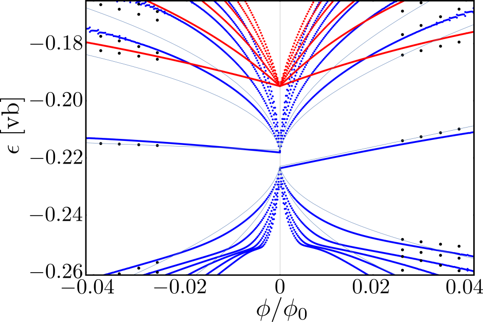
Figure 3: The Landau level spectra of the valence band secondary Dirac point (sDP) the perturbation $u_{0,1,3}=\{0.032,-0.063,-0.055\}$, obtained from either Hamiltonian (52) for the $\kappa^{\prime}$ and $\kappa$ corners (red and blue dots) or Hamiltonian (6) (black dots). The grey solid lines are the Landau levels of the effective Hamiltonian, Eq. (61), using fitted parameters $E_{0}=-0.22vb$, $\Delta_{\kappa}=-0.0057vb$, $\tilde{v}=0.38v$, $\bar{M}=-0.97ev/b$, and $\tilde{M}=-1.45ev/b$.

Here we give an analytical description of the almost gapless sDP found at the corner superlattice Brillouin zone in the valence band in the top row of Fig. 1. To do this, we note that zone folding using Bragg vectors $\bm{b}_{m}$ brings together three degenerate plane wave states $|\zeta\!\bm{\kappa}\rangle$, $|\zeta\!(\bm{\kappa}+\bm{b}_{2})\rangle$ and $|\zeta\!(\bm{\kappa}+\bm{b}_{1})\rangle$to each of the two inequivalent corners of the moiré Brillouin zone where $\zeta=\pm 1$, $\bm{\kappa}=(\bm{b}_{4}+\bm{b}_{5})/3$, and,

$$|\zeta\bm{p}\rangle=\frac{1}{\sqrt{2}}\left(\begin{array}[]{c}1\\ -\alpha e^{2i\varphi}\end{array}\right)e^{i\zeta\bm{p}.\bm{r}},$$ (50)

with $\varphi$ the polar angle of momentum $\zeta\bm{p}$, and $\alpha=\pm 1$ the band index. Using $\bm{k}\cdot\bm{p}$ theory, the vicinity of each moiré Brillouin zone corner can then be described using an effective Hamiltonian acting on a three component vector of smoothly varying envelope functions, written in a basis of the standing wave states,

$$\Phi_{1}\!=\!\frac{1}{\sqrt{3}}\left(|\zeta\!\bm{\kappa}\rangle+|\zeta\!(\bm{\kappa}+\bm{b}_{2})\rangle+|\zeta\!(\bm{\kappa}+\bm{b}_{1})\rangle\right),$$ (51)

$$\Phi_{2}\!=\!\frac{1}{\sqrt{3}}\left(e^{i\pi}|\zeta\!\bm{\kappa}\rangle+e^{\text{-}i\frac{\pi}{3}}|\zeta\!(\bm{\kappa}+\bm{b}_{2})\rangle+e^{i\frac{\pi}{3}}|\zeta\!(\bm{\kappa}+\bm{b}_{1})\rangle\right),$$

$$\Phi_{3}\!=\!\frac{1}{\sqrt{3}}\left(e^{\text{-}i\pi}|\zeta\!\bm{\kappa}\rangle+e^{i\frac{\pi}{3}}|\zeta\!(\bm{\kappa}+\bm{b}_{2})\rangle+e^{\text{-}i\frac{\pi}{3}}|\zeta\!(\bm{\kappa}+\bm{b}_{1})\rangle\right).$$

Using basis (51) the $\bm{k}\cdot\bm{p}$ Hamiltonian for the $K$-valley is diagonal exactly at the Brillouin zone corner,

$$\hat{\bm{H}}_{K}(\zeta,\bm{p},\bm{B})$$ (52)

$$=\!\!\!\left(\!\begin{array}[]{ccc}\hat{\bm{\epsilon}}_{0}\!+\!\epsilon_{1}\!\!&\tilde{v}\hat{\bm{\pi}}^{\dagger}&\tilde{v}\hat{\bm{\pi}}\\ \tilde{v}\hat{\bm{\pi}}&\!\!\hat{\bm{\epsilon}}_{0}\!+\!\epsilon_{2}\!\!&\!-\!\tilde{v}\hat{\bm{\pi}}^{\dagger}\\ \tilde{v}\hat{\bm{\pi}}^{\dagger}&\!-\!\tilde{v}\hat{\bm{\pi}}&\!\!\hat{\bm{\epsilon}}_{0}\!+\!\epsilon_{3}\end{array}\!\right)\!$$ (56)

$$\,\,+\tilde{v}\!\left(\!\begin{array}[]{ccc}0&\!\!\!\!-\!(\eta_{1}\!+\!\eta_{2}\!+\!\eta_{3})\hat{\bm{\pi}}^{\dagger}\!\!&\!\!(\eta_{2}\!-\!\eta_{3})\hat{\bm{\pi}}\\ \!-\!(\eta_{1}\!+\!\eta_{2}\!+\!\eta_{3})\hat{\bm{\pi}}\!\!&0&\!\!\!-\!(\eta_{1}\!+\!2\eta_{3})\hat{\bm{\pi}}^{\dagger}\\ (\eta_{2}\!-\!\eta_{3})\hat{\bm{\pi}}^{\dagger}\!\!&\!\!\!-\!(\eta_{1}\!+\!2\eta_{3})\hat{\bm{\pi}}\!\!&0\\ \end{array}\!\right)\!;$$ (60)

$$\epsilon_{1}=2\Re W,\ \epsilon_{2}=-\Re W+\sqrt{3}\Im W,\ \epsilon_{3}=-\Re W-\sqrt{3}\Im W,$$

$$W\!\approx\!\frac{vb}{2}(u_{0}\!+\!i\zeta u_{3})\!+\!\frac{v^{3}b^{3}}{6\gamma_{1}^{2}}e^{\frac{2i\pi}{3}}(u_{0}\!-\!i\zeta u_{3})\!+\!\frac{\alpha\zeta v^{2}b^{2}}{\sqrt{3}\gamma_{1}}e^{\frac{\text{-}2i\pi}{3}}u_{1},$$

$$\hat{\bm{\epsilon}}_{0}\!=\!\frac{\alpha v^{2}b^{2}}{3\gamma_{1}}\!+\!\frac{\alpha v^{2}}{\gamma_{1}}\hat{\bm{p}}^{2},\quad\tilde{v}\!=\!\zeta\alpha\frac{bv^{2}}{\sqrt{3}\gamma_{1}},\quad\eta_{3}=\frac{1}{2}\sqrt{3}\zeta\mu_{1}$$

$$\eta_{1}=\frac{vb\left(\sqrt{3}\zeta\mu_{3}+\mu_{0}\right)}{2\gamma_{1}},\eta_{2}=\frac{vb\left(\mu_{0}-\sqrt{3}\zeta\mu_{3}\right)}{2\gamma_{1}},$$

where $\Re$ and $\Im$ denote the real and imaginary parts. The corresponding Hamiltonian for the $K^{\prime}$-valley is obtained using time reversal symmetry, $\hat{\bm{H}}_{K}(\zeta,\bm{p},\bm{B})$=$\hat{\bm{H}}^{*}_{K^{\prime}}(\text{-}\zeta,\text{-}\bm{p},\text{-}\bm{B})$.

Figure 3 shows the LL spectra of Hamiltonian (52) using blue(red) dots for the $-\kappa$($\kappa$) corner, where the signature of an almost gapless sDP is evident at $\epsilon\approx-0.22\,vb$ for the $-\kappa$ corner. To calculate this spectra, we diagonalized the Heisenberg matrix of Hamiltonian (52) in a basis consisting of the products of magnetic oscillator functions (14) with the standing waves states (51), $\varphi_{n}(k_{2})\Phi_{i}$, where we take $i=1,2,3$, and $n=0\cdots n_{\text{max}}$, where is $n_{\text{max}}$ sufficiently large that the resulting spectrum converges. Any eigenstates with a large weight on high-index magnetic oscillator functions, $\varphi_{n}(k_{2})$ with $n\gtrsim(b\lambda_{B})^{2}$, are discarded because they violate the $\bm{k}\cdot\bm{p}$ approximation used to construct Hamiltonian (52). Also, to improve the comparison of its LL spectra with that of Hamiltonian (6), we calculate the moiré perturbation correction to the band-edge energies, $\epsilon_{1,2,3}$, using a higher order of perturbation theory than is explicit in Eq. (52).

The result of numerical diagonalization of the two band Hamiltonian (6) is displayed using black dots in Fig. 3. The two spectra agree well, confirming that Eq. (52) is a good description of the sDP. Moreover, we can diagonalize Hamiltonian (52) for arbitrarily small magnetic fields, where the size of the Heisenberg matrix of magnetic Bloch functions (21) needed to diagonalize Hamiltonian (6) becomes prohibitively large.

The energy of the“zeroth” LL originating from the sDP in Fig. 3 depends on the magnetic field, due to a non-zero magnetic momentum generated from the influence of a third band (residing mainly on $\Phi_{3}$ for Hamiltonian (52)) that mixes with the LLs of the first two bands. For the parameter set $u_{0,1,3}=\{0.032,-0.063,-0.055\}$, this third band is separated by a large gap from the sDP, which permits the approximate two band description for the sDP,

$$\hat{\bm{H}}_{\text{sDP}}^{\text{eff}}\!=\!E_{0}\!+\!\frac{\Delta_{\kappa}}{2}\sigma_{3}\!+\!\tilde{v}\hat{\bm{p}}\cdot\bm{\sigma}\!-\!\left(\bar{M}+\tilde{M}\sigma_{3}\right)\!B.$$ (61)

where the parameters for the energy shift $E_{0}$, gap $\Delta_{\kappa}$, effective velocity $\tilde{v}$, and magnetic momentums $M$ and $\tilde{M}$ can be fitted to the result of numerically diagonalizing Eq. (6). Such a fitting is illustrated in Fig. 3 using the grey lines, and produces the best accuracy for low indexed LLs.

IV Magnetic miniband spectrum and compressibility of 2D electron liquid in BLG-hBN heterostructures

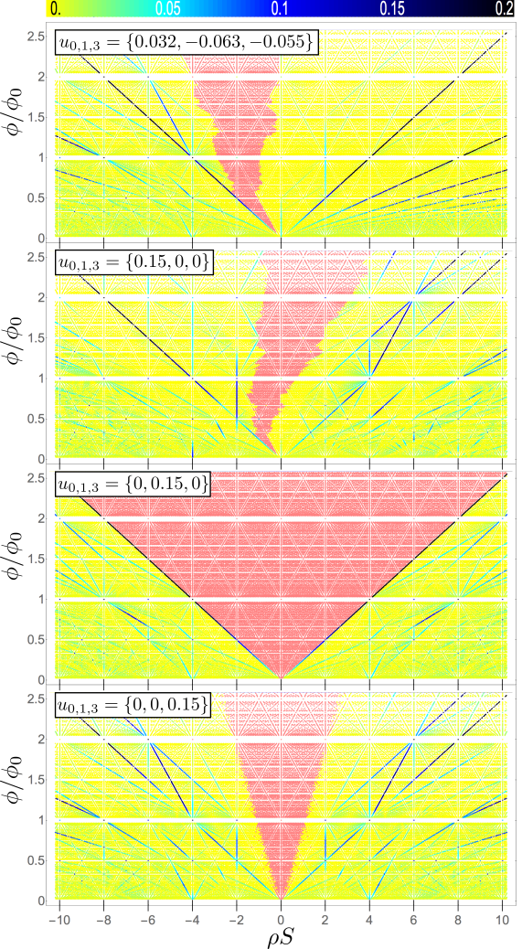
Figure 4: Density-magnetic field diagram showing incompressible electron states in the magnetic minibands, calculated for the same parameters as Fig. 1. Larger gaps are shown using a darker color, yellow represents a vanishing gap, and red represents the particular gapless states associated with the zero-energy Landau level.

Fig. 4 shows the maps of incompressible states for each parameter set in Fig. 1, created by filling the corresponding magnetic miniband spectrum with electrons. A larger gap is depicted with a darker color, resulting in lines, the gradient of which corresponds to the filling factor. For the regions shown in yellow, the gap is negligibly small as a result of incomplete filling of a magnetic miniband, each of which can accommodate a density $\delta\rho=1/(\pi p\lambda_{B}^{2})$ of electrons (including spin degeneracy). In contrast, the unperturbed zero-energy Landau level present in the $K^{\prime}$ valley accommodates electron density of $\delta\rho_{0}=1/(\pi\lambda_{B}^{2})$, creating a large gapless region portrayed in red. Because of its large electron capacity at exactly zero energy, the presence of this zero-energy mode should be clearly visible in capacitance measurements. Electron-hole symmetry is displayed in the plots for $u_{0,1,3}=\{0,0.15,0\}$ (lower left), and $u_{0,1,3}=\{0,0,0.15\}$ (lower right), whereas it is absent in the upper two plots.

Many of the largest gaps in the magnetic spectrum plots (Fig. 1) occur between the zeroth and first LLs of Dirac points (whether original or secondary). In the map of incompressible states, these large gaps are manifest as a solid blue line, which intersect the $B=0$ axis at a density $\rho S=4m$, where $m=0$ for the main Dirac point or $m=\pm 1$ for an sDP at the edge of the first conduction/valence miniband. For example, there is a (gapped) sDP in the valence band of the magnetic spectrum for the moiré perturbation $u_{0,1,3}=\{0.032,-0.063,-0.055\}$ (upper panel in Fig. 1). In the upper panel of Fig. 4, the gap between the two zeroth LLs of this sDP is represented as a blue vertical line, which starts from ($\rho S=-4$, $B=0$), whereas the two gaps between the zeroth and first LLs are shown as two tilted blue lines, with gradients of $\pm 2$.

V Conclusions

In summary, we have shown that the presence of the hBN substrate lifts the valley degeneracy of bilayer graphene, producing different magnetic Hofstadter’s butterflies in each valley. The zero-energy Landau level located on the layer furthest from the hBN substrate remains unaffected by the moiré perturbation, which makes the BLG/hBN spectrum unique in comparison to other known magnetic spectra, for which all Landau levels split into sub-bands. We investigated the influence of different possible characteristics of moiré perturbation including an electrostatic potential which does not distinguish between the two carbon sublattices, a sublattice-asymmetric part of the potential, and a spatial modulation of the nearest-neighbor carbon-carbon hopping amplitude, and we identified how they give rise to different features in the electronic spectra including gapped or overlapping bands, or bands connected by a secondary Dirac point. In addition to determining the fractal electronic spectra by numerical diagonalization of a model Hamiltonian, we also derived simple effective Hamiltonians to describe low-energy features in the magnetic minibands and to describe the secondary Dirac point. Finally, we showed how gaps in the fractal energy spectrum lead to the formation of incompressible states that may be observed under a variation of carrier density and magnetic field.

- (1) L. A. Ponomarenko, R. V. Gorbachev, G. L. Yu, D. C. Elias, R. Jalil, A. A. Patel, A. Mishchenko, A. S. Mayorov, C. R. Woods, J. R. Wallbank, M. Mucha-Kruczyński, B. A. Piot, M. Potemski, I. V. Grigorieva, K. S. Novoselov, F. Guinea, V. Fal’ko and A. K. Geim, Nature 497, 594 (2013).
- (2) C. R. Dean, L. Wang, P. Maher, C. Forsythe, F. Ghahari, Y. Gao, J. Katoch, M. Ishigami, P. Moon, M. Koshino, T. Taniguchi, K. Watanabe, K. L. Shepard, J. Hone, P. Kim, Nature 497, 598 (2013).
- (3) B. Hunt, J. D. Sanchez-Yamagishi, A. F. Young, M. Yankowitz, B. J. LeRoy, K. Watanabe, T. Taniguchi, P. Moon, M. Koshino, P. Jarillo-Herrero, R. C. Ashoori, Science 340, 1413 (2013).
- (4) E. Brown, Phys. Rev. 133, A1038 (1964).
- (5) J. Zak, Phys. Rev. 134, A1602 134, A1607 (1964).
- (6) J. Zak, Phys. Rev. 134, A1607 134, A1607 (1964).
- (7) D. R. Hofstadter, Phys. Rev. B 14, 2239 (1976).
- (8) G. L. Yu, R. V. Gorbachev, J. S. Tu, A. V. Kretinin, Y. Cao, R. Jalil, F. Withers, L. A. Ponomarenko, B. A. Piot, M. Potemski, D. C. Elias, X. Chen, K. Watanabe, T. Taniguchi, I. V. Grigorieva, K. S. Novoselov, V. I. Fal’ko, A. K. Geim and A. Mishchenko, Nat. Phys 10, 525 (2014)
- (9) L. Wang, Y. Gao, B. Wen, Z. Han, T. Taniguchi, K. Watanabe, M. Koshino, J. Hone, C. R. Dean, Science 350, 1231 (2015).
- (10) J. R. Wallbank, A. A. Patel, M. Mucha-Kruczyński, A. K. Geim, and V. I. Fal’ko, Phys. Rev. B 87, 245408 (2013).
- (11) X. Chen, J. R. Wallbank, A. A. Patel, M. Mucha-Kruczyński, E. McCann, and V. I. Fal’ko, Phys. Rev. B 89, 075401 (2014).
- (12) M. Diez, J. P. Dahlhaus, M. Wimmer, and C. W. J. Beenakker, Phys. Rev. Lett. 112, 196602 (2014).
- (13) P. Moon and M. Koshino, Phys. Rev. B 90, 155406 (2014).
- (14) L. A. Chizhova, F. Libisch, and J. Burgdörfer, Phys. Rev. B 90, 165404 (2014).
- (15) J. R. Wallbank, M. Mucha-Kruczyński, X. Chen, and V. I. Fal’ko, Ann. Phys. 527, 359 (2015).
- (16) G. J. Slotman, M. M. van Wijk, Pei-Liang Zhao, A. Fasolino, M. I. Katsnelson, and Shengjun Yuan Phys. Rev. Lett. 115, 186801 (2015).
- (17) R. Bistritzer and A. H. MacDonald, Phys. Rev. B, 84, 035440 (2011).
- (18) J. M. B. Lopes dos Santos, N. M. R. Peres, and A. H. Castro Neto, Phys. Rev. Lett. 99, 256802 (2007).
- (19) E. McCann and V. I. Fal’ko, Phys. Rev. Lett. 96, 086805 (2006).
- (20) R. S. Deacon, K.-C. Chuang, R. J. Nicholas, K. S. Novoselov, and A. K. Geim, Phys. Rev. B 76, 081406 (2007).
- (21) A. B. Kuzmenko, I. Crassee, D. van der Marel, P. Blake, and K. S. Novoselov, Phys. Rev. B 80, 165406 (2009).
- (22) M. Mucha-Kruczyński, J. R. Wallbank and V. I. Fal’ko, Phys. Rev. B 88, 205418 (2013).
- (23) J. Xue, J. Sanchez-Yamagishi, D. Bulmash, P. Jacquod, A. Deshpande, K. Watanabe, T. Taniguchi, P. Jarillo-Herrero, and B. J. LeRoy, Nat. Mater. 10, 282 (2011).
- (24) A. Ghazaryan and T. Chakraborty, Phys. Rev. B 92, 235404 (2015).
- (25) X. Chen and V. I. Fal’ko, Phys. Rev. B 93, 035427 (2016).