From A to Z: Supervised Transfer of Style and Content Using Deep Neural Network Generators

Abstract

We propose a new neural network architecture for solving single-image analogies—the generation of an entire set of stylistically similar images from just a single input image. Solving this problem requires separating image style from content. Our network is a modified variational autoencoder (VAE) that supports supervised training of single-image analogies and in-network evaluation of outputs with a structured similarity objective that captures pixel covariances. On the challenging task of generating a 62-letter font from a single example letter we produce images with 22.4% lower dissimilarity to the ground truth than state-of-the-art.

1 Introduction

Separating image style from content is an important problem in vision and graphics. One key application is analogies: if we can separate an image into style and content factors, we can generate a new image by holding style fixed and modifying the content (resulting in an image with different semantics but the same style), or vice versa. For instance, given a letter ‘A’ the goal would be to generate all of the letters ‘B’, ‘C’, … in the same style. Or, given a stylized image (e.g., Instagram filtered), the goal could be to recover the unfiltered image or switch to a different filter.

We call this kind of analogy a single-image analogy since only a single image is given as input. Clearly, producing ‘B’ given only ‘A’ is impossible without drawing on some prior knowledge, so learning a prior over either style or content will play a role in solving single-image analogies.

Kingma et al [13] observed that deep neural networks can learn latent spaces in which reasoning about single-image analogies is possible. Style is implicitly preserved in the organization of the learned embedding space. They produce compelling results, yet they did not directly optimize for preserving style or producing analogies, nor do they quantitatively evaluate the analogies they produce.

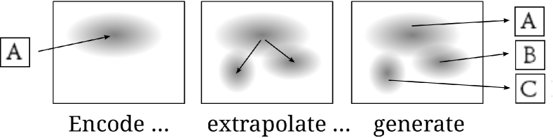
Figure 1: Analogical reasoning. This figure illustrates how our method produces a font from a single letter. First, the input image (e.g., ‘A’) is encoded to a Gaussian distribution in a latent space. Next we extrapolate the latent distribution to new latent distributions which describe other letters of the same font. Finally, we generate new images by sampling each latent distribution and mapping the sampled point to an image.

We extend the work of [13] by introducing a new deep neural network architecture for better single-image analogies. Our key insight is that having training data grouped into style sets (a sequence of images with known content and consistent style) allows direct optimization of a style embedding space and reasoning about single-image analogies.

We demonstrate our method on a new, large-scale dataset of 1,839 fonts. We experiment on 10-class digits and 62-class alphanumerics and show that our method consistently outperforms previous work under a variety of experimental settings. Though our demonstration application is font generation, our architecture is not specific to any domain.

Our insight is to train on supervised style sets and optimize for image quality. Thus, our contributions are:

• A neural network model [13]: Our model has a latent distribution extrapolation layer and two adversarial networks [10] (class and imposter discriminators).

• Improved image quality with SSIM [31]: Our model optimizes generated images for structured similarity (i.e., pairwise pixel covariances) to ground truth.

• A challenging image analogy dataset: Our dataset has more classes, more styles and more subtle style cues compared to MNIST [16] and Street View House Numbers (SVHN) [20].

2 Related Work

Image analogies are part of a larger research area of image generation which has attracted much attention. Image analogies support a variety of applications (e.g., super-resolution, texture transfer, texture synthesis and automatic artistic filtering). The generalized image analogy problem can be phrased as “A is to B as C is to D”. The goal is to produce image D.

We first describe works which require A, B and C as image inputs. Hertzmann et al [12] proposed a method where they suppose the pixelwise content of (A, B) and (C, D) pairs are nearly identical. Thus, they dynamically construct a high-quality D by finding pixelwise matches and transferring style. Under similar constraints, Memisevic and Hinton [18] proposed an unsupervised model which learns the image transformations. Taylor et al [27] present a third-order restricted Boltzmann machine (RBM) which can generate analogs without requiring (A, B) and (C, D) pairs to be pixelwise dependent. Although not intended for images, the word2vec project [19] found that learned latent spaces can easily solve analogical reasoning tasks. Sadeghi et al [26] do not generate images but they learn a latent space for solving analogy queries.

A parallel work by Reed et al [25] develop a deep neural network for visual analogies with three input images. They propose three forms of extrapolation and a disentangled feature representation.

Recently, Gatys et al [9] have proposed a scalable, high-quality method which uses the layered features of a deep convolutional neural network (CNN) to separate content from style. They do not require image A. Given only images B and C, they produce an image D which matches the content of C and the style of B. They draw upon knowledge learned by training a CNN on over 1 million images.

Single-image analogies are possible. To our knowledge, only Kingma et al [13] claim to produce style and content factored image analogies from a single image. Given only image B they produce digits which match the style of B while adhering to a specified content class (restricted to content classes which have been seen during training). Tenenbaum and Freeman [28] propose an extrapolation method that produces letters of a font given only examples of other letters of the same font. However, they only demonstrate results when 53 input letters are provided.

Kulkarni et al [15] present an inverse graphics model that disentangles pose and lighting. They propose a novel training procedure for factoring their latent space.

Using SSIM as an optimization target is not a new idea [32, 7, 22]. Indeed, much work as been done on analysis of the quasi-convexity of SSIM [6, 4]. Regarding generative models, Ranzato and Hinton [23] first argued that capturing dependencies between pixels is important. Subsequently, there have been models which aim to capture pairwise dependencies in natural images [24, 8, 11].

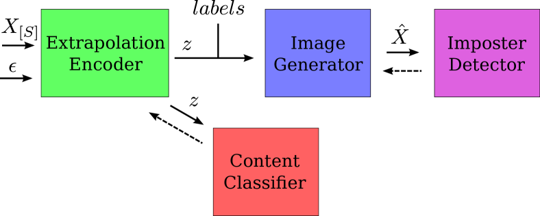
Figure 2: Model overview. The variational encoder (green) takes a subset of the style set images $X_{[S]}$ (example shown) and a noise variable $\epsilon\sim\mathcal{N}(0,I)$ as input, and produces code $z$ for all members of the style set, and combines the codes with identity class labels. The generator (blue) to image reconstructions $\hat{X}$ (example shown) for the entire style set. An imposter detector adversary (purple) is used to improve the reconstruction quality. An identity classifier adversary (red) is used to promote class invariance on $z$ codes. Dotted lines indicate zones which update weights with a negated gradient wrt loss functions in the adversarial zones.

3 Overview

At its core, our method is an encoder / decoder pair (Figure 1). The encoder takes an image and maps it to a point in a $Z$-dimensional embedding space $\mathbb{R}^{Z}$ (aka a latent space). Our method enforces structure on this space: it represents only style, but not content. The decoder combines style information from the embedding space with a content switch variable. For example, if our domain is fonts, and we feed in ‘A’ to the encoder, we get a point in the embedding space $\mathbb{R}^{Z}$ representing the style of ‘A’. If we pass this point to the decoder, but with the content switch ‘B’, then the decoder should produce ‘B’—the letter ‘B’, but in the style of ‘A’.

We now describe our key contributions: a deep neural network architecture, in-network and out-of-network image quality assessment measures, and a new font dataset with high-quality ground truth for analogical reasoning.

Network architecture. Our neural network is a modified variational autoencoder (VAE) [14, 13], a state-of-the-art semi-supervised image generator. We introduce VAEs here and briefly review their mathematics in Section 5.1.

A VAE encoder is trained to learn a mapping from images to latent codes. These codes are not points, but rather multivariate Gaussians. Mapping images to distributions conditions the latent space [14]. The encoder must learn a mapping where differing images rarely overlap. This yields a better organized latent space. We then sample from a latent code to get a latent point that we can feed to the decoder.

Kingma et al. [13] demonstrated a conditional decoder model that can produce image analogies for MNIST and SVHN digits. Their decoder takes both a latent point and a content variable (i.e., ‘1’, ‘2’, ‘3’, etc.), and is trained to produce styled images of the specified content. This structure naturally lends itself to producing complete sets of digits, given a single example.

Our idea is to use supervision to learn analogies. Since (in the case of fonts) the content labels (‘A’, ‘B’, …) are available for all training examples, we want to use those labels to learn to generate an entire style set (given some subset as examples). Our modifications to the standard VAE model are natural consequences of this key idea. As we describe each change in the following paragraphs, we refer the reader to the colored zones in Figure 2, which shows a high-level overview of the network. Also, components of our model are described mathematically in Section 5.

Extrapolation Layer. Our input is only a subset of the style set so the latent codes for the entire subset must be extrapolated. In our model we extrapolate by taking linear combinations of the latent means and variances of the subset images to produce a latent mean and variance for each member of the style set. This gives our model more expressive power than [13] which holds the latent mean and variance constant across all members. We call our method an extrapolation layer and find that gives a significant increase in performance.

SSIM Cost Function. The VAE conditional decoder (Figure 2 blue zone) generates a complete style set by combining latent codes (sampled from the latent distributions) with class labels. Since pairwise pixel interactions are important in human perception and modeling images [23], our idea is to use an objective function based on SSIM [30], an image quality measure that captures pairwise dependencies. We describe our objective function in Section 5.4 and compare against an $L_{2}$ objective in Section 6.4.

Adversarial Sub-Networks. Ideally, the latent space should be a style embedding. Image content should come from the content variable we pass to the decoder — not from the latent code. We factor content out of the latent space with an adversarial [10] content classifier connected to the encoder by a gradient reversal layer [33] (Figure 2 red zone). Gradient reversal layers render a latent space invariant to a domain during training. We explain how this works in Section 5.5 and we find it gives a small performance improvement (Section 6.6). We also experimented with adding an adversarial imposter detector to improve the visual quality of the generated output (Figure 2 purple zone, Section 5.6).

A new dataset for quantitative evaluation. We require training data with both style and content annotations. Fortunately, human designers have deliberately created a multitude of complete sets of stylistically consistent fonts. Furthermore, these have subtle, challenging style variations. It may seem overly challenging to generate an entire font from a single letter, but this has been demonstrated by [5] (although they use domain-specific knowledge). Compared to MNIST and SVHN, our dataset has more classes, and emphasizes subtle style cues such as curvature, stroke, width, slant, and serifs. We describe our dataset further in Section 4.

Evaluation. We give extensive quantitative comparisons of our method to variational autoencoders in Section 6. Our method outperforms standard variational autoencoders under many conditions. For qualitative evaluation, we offer many analogical reasoning examples in Figures 5, 6, 7, and 8.

We also perform experiments to justify our modifications to the VAE model. We investigate the changes in performance when the extrapolation layer and adversarial discriminators are removed from the network. Those experiments are described in Section 6.3 and 6.6.

Finally, we do not use domain-specific knowledge, so our model is extensible to other domains.

4 Font Dataset

Figure 3: Font dataset. Top four rows: subsets of selected decorative, script and blackletter fonts to illustrate the variety of styles present in the dataset. Bottom: the average font, which looks normal since the majority of fonts are serif or sans serif.

We have created a dataset of 1,839 fonts to provide quality ground truth for analogical reasoning. We used fonts from openfontlibrary.org as well as the fonts used by [21]. Our dataset includes serif, sans serif, blackletter, calligraphic, script and decorative font styles. From each font we produce a style set of 62 images—26 uppercase letters, 26 lowercase letters and 10 digits.

We ensure each font is unique by eliminating any duplicate image sets. However, duplicate letters may still exist, which would add unwanted bias to our dataset. We address this by clustering letters: We merge two clusters if at least one pair of letters (1) are identical or (2) come from the same file (professional font creators often store related fonts together) or (3) have the same font family (based on metadata in the font file). We selected a random subset of clusters such that 191 fonts were in the test set. Of the remainder we use 92 fonts for validation and 1,556 for training. There are 102,176 training samples and 11,842 testing samples.

Our dataset is of a comparable size to MNIST, but contains 6.2 times as many classes, as well as some unusual styles. The dataset average is similar to a typical sans serif font. See Figure 3 for selected examples of the different styles. Note that the decorative fonts in the first and third rows would be difficult to generate with the method of [5], which relies on outline alignment.

On our dataset, successful analogical reasoning is well-defined. For example, if given the image of letter ‘A’ from Arial and asked to produce a ‘B’, then the unique correct answer is the Arial image of letter ‘B’.

5 Neural Network Model

In this section we mathematically define our problem and describe the components of our model. Let $X$ be a complete, ground truth style set of $M$ images. Let $X_{[S]}$ be a specific subset of $X$ (e.g., if we select $S=\{\text{`A'}\}$ then the given letter is always letter ‘A’). Given only $X_{[S]}$ we will generate $\hat{X}$, a reconstruction of the entire style set. The goal is to minimize the dissimilarity of $\hat{X}$ and $X$.

Our model can be divided into four zones as depicted in Figure 2. The purpose of each zone is described in Section 3. The green zone is a variational encoder and extrapolation layer that produces latent codes given images. The blue zone is an image generator (aka a decoder) that produces an image when given a latent code and a class label. The purple zone is a discriminator trained to detect image imposters. The red zone is an $M$-way classifier trained to detect which class produced a given latent code.

Figure 4: Extrapolation encoder and image generator. Left: The extrapolation encoder produces two sets of latent distributions. One set ($z_{1}$) corresponds to a standard VAE encoder. The second set ($z_{2}$) is produced by our extrapolation layer (shaded portion). See Sections 5.1, 5.2 for details. Right: The image generator produces images for both sets of codes. All generated images are compared against ground truth. The $z_{2}$ images are the analogical reasoning output. See Section 5.3.

5.1 Variational encoder

The encoder takes an image $x$ and produces a latent code $z$ (Figure 4). In particular, we describe the encoder as a function $g$ which maps $x$ to $\mathcal{N}(\mu,\Sigma)$, a multivariate normal distribution. $\Sigma$ is a diagonal covariance matrix — its diagonal is the vector $\sigma^{2}$. The latent code is $z\sim g(x)\in\mathbb{R}^{Z}$.

We implement $g(x)$ as a multilayer perceptron with two hidden layers of 500 nodes and scaled hyperbolic tangents [17]: $h(a)=1.7159\tanh\frac{2}{3}a$. The activations of the output layer is called the hidden encoder state, $h_{enc}$. We extract $\mu$ and $\sigma$ from $h_{enc}$ as $\mu=h_{enc}W_{1}+b_{1}$ and $\log\sigma=\frac{1}{2}(h_{enc}W_{2}+b_{2})$ where $W_{i}$ and $b_{i}$ are learned weights and biases. Then a reparameterization is $z=\mu+\sigma\epsilon$ ($\sigma$ and $\epsilon$ are multiplied element-wise). $\epsilon\sim\mathcal{N}(0,I)$ is an auxilliary noise variable. We take the latent distribution prior to be an isotropic Gaussian $\mathcal{N}(0,I)$. Then the deviation of a latent distribution from the prior is the KL divergence, $D_{KL}(\mathcal{N}(\mu,\sigma^{2})\;||\;\mathcal{N}(0,I))$. This is an objective function for our model which regularizes learned latent distributions. The encoder loss is

$$L_{enc}=-\frac{1}{2}\sum 1+2\log\sigma-\mu^{2}-\sigma^{2}.$$

During training, every member of a style set is encoded as $z_{1}=g(X)\in\mathbb{R}^{M\times Z}$. The preceeding summarizes how latent codes are produced by a standard VAE and we refer the reader to [14] for details. Our network also produces $z_{2}$, extrapolated codes from a subset of $X$.

5.2 Extrapolation layer

The extrapolation layer takes subsets of $\mu$ and $\sigma$ and extrapolates them to cover every member of our style set. Let $\mu_{[S]}\in\mathbb{R}^{K\times Z}$ be the subset of $\mu$ corresponding to $X_{[S]}$ and likewise for $\sigma_{[S]}$. We introduce a linear mixing layer that takes $K$ latent distributions, mixes them and generates $M$ latent distributions which are sampled to get latent codes. The mixture is $\mu_{mix}=W_{3}\mu_{[S]}$ and $\sigma_{mix}=W_{4}\sigma_{[S]}$ where $W_{3}$ and $W_{4}$ are $M\times K$ matrices. Then $z_{2}=\mu_{mix}+\sigma_{mix}\epsilon\in\mathbb{R}^{M\times Z}$. The extrapolation layer allows the model to fit a latent distribution to each member of the style set.

5.3 Image generator

The image generater maps $(z,label)$ to an image $\hat{x}$ (Figure 4). $z$ is a latent code and $label$ is a conditional variable (one of $M$ classes, one-hot encoded) which controls the content of the output. We implement $f$ as a three-layer multilayer perceptron which takes the concatenation of $z$ and $label$ as the input vector. The hidden layers (500 nodes) have scaled hyperbolic tangents and the output layer has a sigmoid nonlinearity. The output layer has a number of nodes equal to $D$, the product of the image dimensions. We apply $f$ to both $z_{1}$ and $z_{2}$ to produce $\hat{x}_{1}=f(g(X))$ and $\hat{x}_{2}=f(z_{2})$. $\hat{x}_{1}$ corresponds to running the model as an autoencoder so we want $\hat{x}_{1}$ to be $X$. The analogical reasoning output of the model is $\hat{X}=\hat{x}_{2}$ which we also want to be $X$. Outputs are compared to $X$ with a structured similarity objective function.

5.4 Structured similarity objective

We want to use SSIM to evaluate image quality. However, calculation of SSIM involves costly Gaussian filtering on local neighborhoods. Instead, we define a global SSIM objective function, $SSIM^{*}$. Its computation depends on global means, $\mu_{1}$ and $\mu_{2}$, biased variances, $\sigma_{1}$ and $\sigma_{2}$, and covariance, $\sigma_{12}$. The similarity of two images, $x_{1}$ and $x_{2}$, is calculated as

$$SSIM^{*}(x_{1},x_{2})=\frac{(2\mu_{1}\mu_{2}+c_{1})(2\sigma_{12}+c_{2})}{(\mu_{1}^{2}+\mu_{2}^{2}+c_{1})(\sigma_{1}^{2}+\sigma_{2}^{2}+c_{2})}$$

where $c_{1}=0.01$ and $c_{2}=0.03$. Our per-channel means and variances are scalars since calculations are summed over all pixels rather than local neighborhoods. We refer the reader to [31] for explanations of the terms. The objective is a similarity measure so we use the negative similarity as the decoder loss function:

$$L_{dec}=-\frac{1}{2}(SSIM^{*}(\hat{x}_{1},X)+SSIM^{*}(\hat{X},X))$$

5.5 Content classifier

We want to be able to alter the content of a generated image so that it differs from that of an input image. This is easily accomplished if $z$ codes are invariant to content (i.e., class). In the case of fonts, this would make the latent space a style embedding. [33] introduced a novel method for using an adversarial network to make an embedding space invariant to domain. We adapt their idea to make our space invariant to content.

The classifier takes a $z$ code and classifies it as one of $M$ classes with a softmax loss, $L_{cls}$. We implement the classifier as a three-layer scaled hyperbolic tangent multilayer perceptron with 500-node hidden layers. The classifier is trained normally, but its gradients are multiplied by $-\lambda$ when they are propagated back to the green zone. We set $\lambda=1$. The intuition behind this gradient reversal is that the weights and biases of the green zone will move so as to make the classification task impossible. If this is achieved then the classifier will be unable to infer content from a $z$ code. A strong indicator that the space is invariant to content.

We train the content classifier on $z_{1}$, the codes from the entire style set. The adversary is trained in a second stage after the encoder and decoder have been trained. Empirically we find that content is easily inferred from $z$ codes (Section 6.6). Regardless, we find that including this adversary improves performance on the test set.

5.6 Imposter detector

We also experimented with applying an adversary to the reconstruction. The intuition is that the imposter detector will learn discriminating visual features and gradient reversals of those detections may provide a supplemental reconstuction loss signal.

The imposter detector is the same architecture as the content classifier. Its two-way softmax loss is $L_{imp}$. We train the imposter detector on minibatches of $X$ and $\hat{X}$ so that it sees an equal number of true and imposter samples.

Overfitting is guaranteed since the detector can memorize the true samples from the training set. Therefore, we test the detector against the validation set and freeze the purple zone weights and biases when performance drops on the validation set.

5.7 Training

We train the network in two stages. The first stage consists of only the encoder and decoder (green and blue zones). The second-stage includes the adversaries. We evaluate validation performance every 10 epochs and stop when loss on the validation set has not improved for 100 epochs. We implement our model in Theano [2, 3] and optimize with SGD with Adagrad learning updates.

First stage. Each minibatch is a complete style set. Therefore, the encoder produces a $z_{1}$ code for every member of the style set. The extrapolation layer is applied to produce the $z_{2}$ codes as mixtures of a subset of the style set. In total $2M$ codes are produced, $M$ codes which correspond directly to each member of the style set, and $M$ codes which are derived from $X_{[S]}$. All codes are concatenated with appropriate class labels and passed to the generator which generates $2M$ images. Half of the images, $\hat{x}_{1}$, correspond to running the network in autoencoder mode (the same as a regular VAE). The other half are $\hat{X}$, the analogical reasoning result. Reconstruction losses are applied to both $\hat{x}_{1}$ and $\hat{X}$. The weighted first-stage loss is:

$$L_{1}=\alpha L_{enc}+\beta L_{dec}$$

Second stage. When the full network is trained its green and blue zones are initialized with weights and biases from a first-stage trained network. The imposter detector receives an input of $2M$ images. Half the images are $\hat{X}$ the other half are $X$. Input images are concatenated with appropriate class labels. The content classifier is given $M$ $z_{1}$ codes, the codes produced by $X$. Training proceeds as normal except after each evaluation the imposter detector is evaluated against the validation set, labeled as non-imposters. It is expected that accuracy on the validation set will rise monotonically. When validation accuracy drops we freeze the purple layer for the rest of training. Aside from freezing those weights, training continues as normal. The weighted second-stage loss is:

$$L_{2}=\alpha L_{enc}+\beta L_{dec}+\gamma L_{cls}+\delta L_{imp}$$

6 Experiments and Results

Model	DSSIM Val	DSSIM Test
M2 [13]	0.1149	0.1276
Ours-SSIM	0.0915 $\pm$ 0.0005	0.1018 $\pm$ 0.0005
Ours-Adv	0.0892 $\pm$ 0.0002	0.0990 $\pm$ 0.0002
Ours-Adv/prior	0.1002 $\pm$ 0.0055	0.1131 $\pm$ 0.0050
Ours-L2	0.0978 $\pm$ 0.0002	0.1089 $\pm$ 0.0003
Ours-Adv/avg	0.0957 $\pm$ 0.0001	0.1011 $\pm$ 0.0028
Ours-Adv/cls	0.0893 $\pm$ 0.0003	0.0994 $\pm$ 0.0003

Table 1: Alphanumeric performance results. Top: We report dissimilarity (mean DSSIM, lower values are better) over 62 alphanumeric classes. Ours-SSIM is our model without the adversaries and Ours-Adv is our full model. See Section 6.1 for details. Bottom: We report performance for variations of our model. Ours-Adv/prior is the full model parameterized to match the prior of M2, Ours-L2 is our model without adversaries and our $SSIM^{*}$ loss replaced with L2, Ours-Adv/avg is our full model but without the extrapolation layer and Ours-Adv/cls is our model without the image imposter adversary.

Model	DSSIM Val	DSSIM Test
M2 [13]	0.0883	0.0923
Ours-SSIM	0.0711 $\pm$ 0.0002	0.0775 $\pm$ 0.0003
Ours-Adv	0.0707 $\pm$ 0.0001	0.0771 $\pm$ 0.0000

Table 2: Digit performance results. We report dissimilarity for 10 digit classes (lower is better). See Section 6.2 for details.

Input letter:	H	Y	f	g	s
DSSIM Val	0.0881	0.0898	0.0990	0.0931	0.0934
DSSIM Test	0.0985	0.1031	0.1081	0.1008	0.1016

Table 3: Input selection. We report dissimilarity on alphanumerics with a randomly selected input class for Ours-Adv. Proper selection of the input class does affect performance. See Section 6.7 for details.

Model	Dataset	$Z$	$\alpha$	$\beta$	$\gamma$	$\delta$
M2 [13]	Alphanum	20
Ours-L2	Alphanum	50	1	100
Ours-SSIM	Alphanum	50	1	$2\times 10^{5}$
Ours-Adv/cls	Alphanum	50	1	$2\times 10^{5}$	200
Ours-Adv	Alphanum	50	1	$2\times 10^{5}$	200	200
Ours-Adv/avg	Alphanum	50	1	$2\times 10^{5}$	200	200
Ours-Adv/prior	Alphanum	50	1	600	200	200
M2 [13]	Digit	20
Ours-SSIM	Digit	20	1	2000
Ours-Adv	Digit	20	1	2000	25	25

Table 4: Model parameters. The parameters of various models used in experiments (Section 6) are described in Section 5.

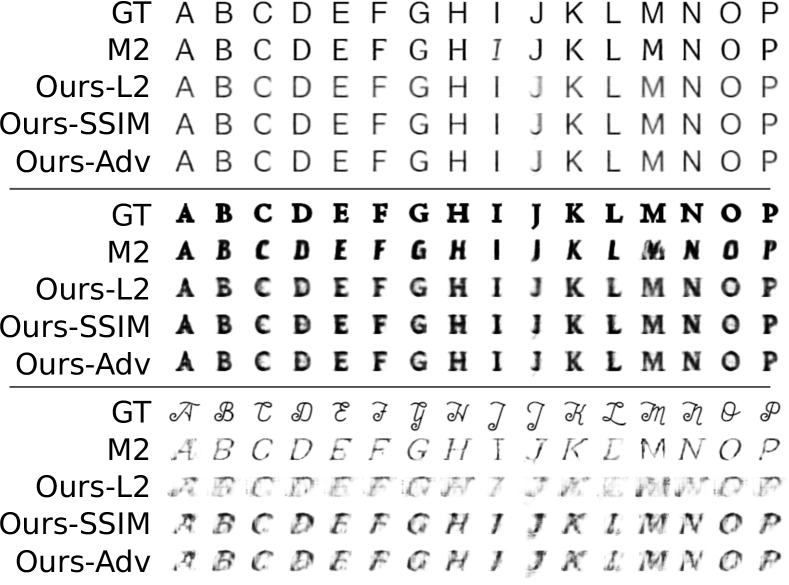
Figure 5: Alphanumeric visual comparisons. We visualize ground truth (GT), VAE (M2) and three variations of our model (Ours-L2, Ours-SSIM, Ours-Adv). The input image is ‘A’. We want to compare fonts that have the same relative quality across models so we ranked the test set for each model then chose fonts which had similar rankings. The first font appears in the top-10 of all four models, the second font appears in the 6 decile and the third font appears in the bottom-10. M2 does not always maintain a consistent slant (e.g., ‘I’ in the first and third fonts) and Ours-L2 is blurry. Ours-Adv has less ghosting compared to Ours-SSIM (e.g., letters ‘C’ and ‘D’, second font).

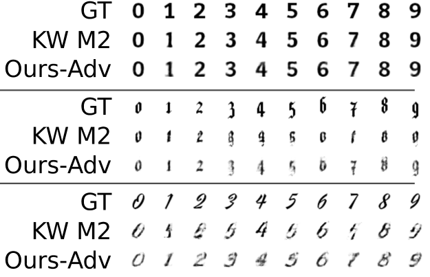
Figure 6: Digit visual comparisons. We visualize ground truth (GT), VAE (M2) and our full model (Ours-Adv). The input image is ‘0’. Fonts were selected as in Figure 5. The first font appears in the top-10 of all four models, the second font appears in the 7 decile and the third font appears in the 2 decile. The odd baseline of the second font is better captured by our model and our ‘1’ for the third font is correctly slanted.

6.1 Alphanumeric performance

To measure performance we report mean DSSIM for the M2 model of [13] (M2), our model without adversaries (Ours-SSIM), and our full model (Ours-Adv).

Mean DSSIM is the mean structural dissimilarity over the set of all images in the style set produced by giving the network one image as input. Here, $DSSIM=(1-SSIM)/2.$ where $SSIM$ is Oliveira’s implementation (means computed on Gaussian filtered neighborhoods) of Wang’s SSIM. Note, the reconstruction of $X_{[S]}$ (the input images) can be trivially perfect by simply echoing back the input rather than using the network outputs. Since we want to evaluate the performance of the network we use the network outputs. This gives a more comprehensive measure of network performance.

Network parameters are given in Table 4. We use a SGD solver with a learning rate of 0.001, weight decay 0.01, momentum 0.9 and L2 weight regularization. The input is $X_{[S]}=\{\text{`A'}\}$.

We test with auxiliary noise variable $\epsilon=0$. Each model was trained three times with different random weight initializations (zero-centered Gaussian, standard deviation 0.01). Biases are initialized to zero. We report the mean and uncertainty of the mean (i.e., $\text{stddev}/\sqrt{3}$). We take weights from the best of the three trials to initialize Ours-Adv for second-stage training.

We find that all variations of our model in all experiments we performed have lower dissimilarity than M2 (see Table 1). It is important to note that [13] did not design their network to solve single-image analogies but rather observed that their model could produce such results. We compare against their model since we qualitatively believe they represent the best state-of-the-art for single-image font analogies. Explicitly, our best model, Ours-Adv, has 22.4% (val) and 22.4% (test) lower dissimilarity compared to M2.

6.2 Alphanumerics versus digits

Our dataset images are high-quality renderings from font definition files and have more than 10 classes. To control for the number of classes we subsampled our dataset to contain only the 10 digit classes. In Figure 6 we compare generated digits versus alphanumerics. We find that having less classes makes for an easier analogy problem with Ours-Adv mean DSSIM dropping by 20.7% (val) and 22.1% (test) compared to alphanumerics. Likewise, M2 dissimilarity drops by 23.2% (val) and 27.7% (test). Results are reported in Table 2 and network parameters are given in Table 4. The validation and test performance gap between our model and M2 (20.0% and 16.5%, respectively) is narrower with 10 classes compared to 62 classes.

6.3 Linear mixing

Do we need our extrapolation layer? If we remove our layer then $z$ codes for missing classes are produced by averaging the $z$ codes of $X_{[S]}$ (when $|S|=1$ this is equivalent to the method of [13] which holds $z$ fixed to produce analogies). We call this variation Ours-Adv/avg in Table 1.

We find that adding our extrapolation layer (Ours-Adv) lowers dissimilarity by 6.79% (val) and 2.08% (test) compared to Ours-Adv/avg.

6.4 L2 versus SSIM

It is known that SSIM is nonconvex [6, 4] — is it possible that L2 is a better optimizing objective even though we evaluate with SSIM? In Table 1 we compare the two objective functions by replacing our $L_{dec}$ (Ours-SSIM) with an L2 loss (Ours-L2). We find that dissimilarity is 6.44% (val) and 6.52% (test) lower with our global SSIM objective.

We also qualitatively compare the results of Ours-L2 to Ours-SSIM in Figure 5. We found pairs for comparison by selecting fonts from the test set which are closely ranked when test fonts are sorted by SSIM for each model. To conserve space we only show 16 alphanumerics.

6.5 Matching the prior

The encoder is an estimator of the prior and the prior loss is an indicator of how dissimilar the estimator is to the prior. M2 may be disadvantaged compared to our model since we favor test set performance over matching the prior. Indeed, our best performing Ours-Adv model has a prior loss of 317.015 (val) whereas M2 is 21.806 (val) on alphanumerics. We can approximately control for prior loss by finding loss weights for our model that produce approximately the same prior loss as M2. We found loss weights for our model (Ours-Adv/prior) such that the prior loss is 20.835 (val). Constrained to matching prior, our model has 12.8% (val) and 11.4% (test) lower dissimilarity than M2.

6.6 Adversaries

We compare a network trained without any adversarial layers (Ours-SSIM) to networks with a class adversary only (Ours-Adv/cls, Table 1) and with both adversary layers (Ours-Adv). We found that adding a class adversary lowers dissimilarity by 2.40% (val) and 2.36% (test). Adding both the class adversary and the imposter adversary lowers dissimilarity by 2.51% (val) and 2.75% (test).

How well does the class adversary impose class invariance on the latent space? The accuracy of the in-network classifier gives us a lower bound on classification accuracy. Chance is 1.6% and Ours-Adv has an accuracy of 85.3% (val). Although, it does not succeed at removing class, it does improve test set performance. It is possible that co-adapted interactions with the extrapolation layer allow class dependence in the latent space.

6.7 Input selection

We arbitrarily selected the first image of the style set as the input image for our experiments (‘A’ for alphanumerics and ‘0’ for digits). How does performance vary with different input images? We ran an experiment on alphanumerics where we varied the input letter of Ours-Adv (‘H’, ‘Y’, ‘f’, ‘g’ and ‘s’ were randomly selected) and found that the best input in that set is ‘H’ and the worst is ‘f’. The dissimilarity of ‘f’ is 12.4% (val) and 9.75% (test) higher than that of ‘H’. Proper selection of the input class can significantly impact performance.

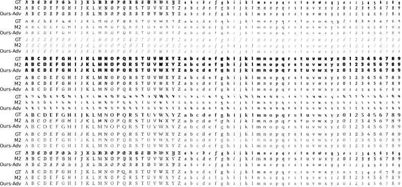
Figure 7: Random visual comparisons. We visualize ground truth (GT), VAE (M2) and our full model (Ours-Adv) on randomly selected test fonts. The input is ‘A’. Our method captures the blackletter style better (first, ninth font). The backwards-slanted sixth font poses problems for both methods. M2 cannot sustain the style of the ‘A’ on the seventh font.

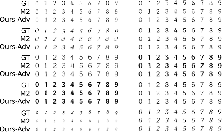
Figure 8: Random visual comparisons. We visualize ground truth (GT), VAE (M2) and our full model (Ours-Adv) on randomly selected test fonts. On many fonts our ‘4’ and ‘7’ are noticeably better. The small font (bottom-left) seems to be challenging for both methods. The thin parts of stokes seem to disappear for M2 (bottom-right font).

7 Discussion and Conclusion

In this paper, we explored a new supervised VAE design for the problem of analogical reasoning of style and content on images. Our experiments show that extrapolating latent distributions outperforms using a fixed latent code for generating image analogies. We also find that having a large number of classes (e.g., all letters and digits) makes for a much more difficult problem compared to a smaller number of classes (e.g., just digits). We also note that using a class adversary leads to slightly improved results.

While our method outperforms the state-of-the-art on our analogies problem, we note that there is significant room for improvement. Our method performs well on standard typefaces, yet on more stylized fonts it can result in blurry or otherwise garbled glyphs, or letters that do not match the style in all respects (e.g., the middle and bottom parts of Figure 5), even though it outperforms prior work. This suggests that this remains a very challenging problem, both because of the stylized nature of the images, and because of the large number of classes; these properties make our dataset compelling for future work. We believe it would be fruitful to explore the role of both more training data and more sophisticated generative models, e.g., convolutional neural networks that factor style and content.

Other domains. In this work we have focused on the domain of fonts. However, our method could be applied to other domains where images can be factored into content and style (or similar factors). Examples of these domains include faces (where images can be decomposed into identity and expression, for instance), images filtered with different Instagram filters, icons in different styles (see for instance thenounproject.com, art, and materials (e.g., learning to transfer textures from one surface to another). In the future we plan to explore these additional domains.

Supplemental

8 Dataset Preparation

The dataset source is 1839 TrueType and OpenType font files. We used FreeType [1] to rasterize the fonts. Each font was rasterized into a 40 $\times$ 40 pixel box on a baseline which is 3/8 of the vertical height. Font sizes were chosen such that each letter of the font fits inside the box (minus a one pixel border) while occupying as much space as possible. Each letter is horizontally translated so that its bounding box is centered horizontally.

9 Visual Comparisons

The main paper has an abridged figure of alphanumeric comparisons. We present the full comparisons in Figure 9. This figure also includes comparisons for multiple inputs (Section 10).

10 Multiple Input

Our model takes any subset $X_{[S]}$ as input. We have limited our main paper experiments to single inputs so we can compare to previous work and because it is a more challenging problem. However, it is interesting to evaluate the effect of multiple inputs (i.e., providing a few example letters). For example, in the case of fonts we could require three samples: uppercase, lowercase, and digit examples. Specifically, we select one input from each subdomain of alphanumerics so that $X_{[S]}=\{\text{`A'},\text{`a'},\text{`0'}\}$. In this case, our extrapolation layer produces new latent distributions as linear mixtures of three latent distributions.

The three-input models (Ours-SSIM/multi and Ours-Adv/multi) have the same training parameters as the single-input models (Ours-SSIM and Ours-Adv). In Table 5 we present our results which show that multiple inputs improve quality. In Figure 9 we find that with multiple inputs the style of the digits match ground truth (GT) better (digits indicated with black arrows in the figure) and the lowercase letters of the second font are crisper (e.g., the loop of ‘d’ and the descenders of ‘j’, ‘p’ and ‘q’, as indicated in the figure).

11 Latent space visualization

In Figure 10 we visualize the latent space with t-SNE [29]. The figure was produced by using t-SNE to project training samples into a 2-D space. The 2-D space was divided into non-overlapping cells and each cell is visualized by the average image of all samples in that cell. Thus, sharp cells contain similar samples and noisy, blurry cells contain multiple dissimilar samples. Generally, we find that the space is organized by visual similarity. This is most clearly seen in the zoomed-in regions of the figure.

Model	DSSIM Val	DSSIM Test
Ours-SSIM	0.0915 $\pm$ 0.0005	0.1018 $\pm$ 0.0005
Ours-Adv	0.0892 $\pm$ 0.0002	0.0990 $\pm$ 0.0002
Ours-SSIM/multi	0.0751 $\pm$ 0.0001	0.0854 $\pm$ 0.0002
Ours-Adv/multi	0.0735 $\pm$ 0.0001	0.0835 $\pm$ 0.0000

Table 5: Multiple input alphanumeric results. Ours-SSIM/multi and Ours-Adv/multi take three letters as input. As expected, dissimilarity is lower with more inputs.

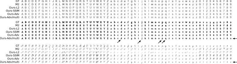
Figure 9: Visual comparisons. We visualize ground truth (GT), single-input VAE (M2), three variations of our single-input model (Ours-L2, Ours-SSIM, Ours-Adv) and our multiple-input model (Ours-Adv/multi). The single input image is ‘A’, the additional inputs are ‘a’ and ‘0’. Test fonts were selected to match Figure 5 of the main paper. The first font appears in the top-10 of all models, the second font appears in the 6 decile and the third font appears in bottom-10. Interesting results for Ours-Adv versus Ours-Adv/multi are marked with black arrows. See Section 10 for details.

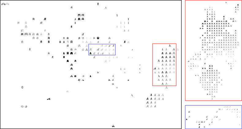
Figure 10: Latent space visualization. Left: We visualize the latent space with gridded t-SNE. Each grid cell contains the average image of all training samples which are in that cell. Generally, we find that similar styles appear grouped. We examine two regions of interest. Top right: This is a zoom-in of the rightmost region of interest. In this region we find both serif and sans serif fonts in separate clusters. Each cluster is organized by stroke weight (heavier fonts at top). Bottom right: This is a zoom-in of the central region of interest. In this region we find the script fonts. They are also organized by stroke weight (heavier fonts to the left).

References

- [1] The FreeType project. http://www.freetype.org/, 2015.
- [2] F. Bastien, P. Lamblin, R. Pascanu, J. Bergstra, I. J. Goodfellow, A. Bergeron, N. Bouchard, and Y. Bengio. Theano: new features and speed improvements. Deep Learning and Unsupervised Feature Learning NIPS 2012 Workshop, 2012.
- [3] J. Bergstra, O. Breuleux, F. Bastien, P. Lamblin, R. Pascanu, G. Desjardins, J. Turian, D. Warde-Farley, and Y. Bengio. Theano: a CPU and GPU math expression compiler. In Proceedings of the Python for Scientific Computing Conference (SciPy), June 2010. Oral Presentation.
- [4] D. Brunet, E. R. Vrscay, and Z. Wang. On the mathematical properties of the structural similarity index. Image Processing, IEEE Transactions on, 21(4):1488–1499, 2012.
- [5] N. D. Campbell and J. Kautz. Learning a manifold of fonts. ACM Transactions on Graphics (TOG), 33(4):91, 2014.
- [6] S. S. Channappayya, A. C. Bovik, C. Caramanis, and R. W. Heath. Design of linear equalizers optimized for the structural similarity index. Image Processing, IEEE Transactions on, 17(6):857–872, 2008.
- [7] S. S. Channappayya, A. C. Bovik, and R. W. Heath. A linear estimator optimized for the structural similarity index and its application to image denoising. In Image Processing, 2006 IEEE International Conference on, pages 2637–2640. IEEE, 2006.
- [8] A. Courville, J. Bergstra, and Y. Bengio. Unsupervised models of images by spike-and-slab rbms. In L. Getoor and T. Scheffer, editors, Proceedings of the 28th International Conference on Machine Learning (ICML-11), ICML ’11, pages 1145–1152, New York, NY, USA, June 2011. ACM.
- [9] L. A. Gatys, A. S. Ecker, and M. Bethge. A neural algorithm of artistic style. arXiv preprint arXiv:1508.06576, 2015.
- [10] I. Goodfellow, J. Pouget-Abadie, M. Mirza, B. Xu, D. Warde-Farley, S. Ozair, A. Courville, and Y. Bengio. Generative adversarial nets. In Advances in Neural Information Processing Systems, pages 2672–2680, 2014.
- [11] T. Hao, T. Raiko, A. Ilin, and J. Karhunen. Gated boltzmann machine in texture modeling. In Artificial Neural Networks and Machine Learning–ICANN 2012, pages 124–131. Springer, 2012.
- [12] A. Hertzmann, C. E. Jacobs, N. Oliver, B. Curless, and D. H. Salesin. Image analogies. In Proceedings of the 28th annual conference on Computer graphics and interactive techniques, pages 327–340. ACM, 2001.
- [13] D. P. Kingma, S. Mohamed, D. J. Rezende, and M. Welling. Semi-supervised learning with deep generative models. In Advances in Neural Information Processing Systems, pages 3581–3589, 2014.
- [14] D. P. Kingma and M. Welling. Auto-encoding variational bayes. arXiv preprint arXiv:1312.6114, 2013.
- [15] T. D. Kulkarni, W. Whitney, P. Kohli, and J. B. Tenenbaum. Deep convolutional inverse graphics network. arXiv preprint arXiv:1503.03167, 2015.
- [16] Y. LeCun, L. Bottou, Y. Bengio, and P. Haffner. Gradient-based learning applied to document recognition. Proceedings of the IEEE, 86(11):2278–2324, 1998.
- [17] Y. LeCun et al. Generalization and network design strategies. Connections in Perspective. North-Holland, Amsterdam, pages 143–55, 1989.
- [18] R. Memisevic and G. Hinton. Unsupervised learning of image transformations. In Computer Vision and Pattern Recognition, 2007. CVPR’07. IEEE Conference on, pages 1–8. IEEE, 2007.
- [19] T. Mikolov, I. Sutskever, K. Chen, G. S. Corrado, and J. Dean. Distributed representations of words and phrases and their compositionality. In Advances in neural information processing systems, pages 3111–3119, 2013.
- [20] Y. Netzer, T. Wang, A. Coates, A. Bissacco, B. Wu, and A. Y. Ng. Reading digits in natural images with unsupervised feature learning. In NIPS workshop on deep learning and unsupervised feature learning, volume 2011, page 5. Granada, Spain, 2011.
- [21] P. O’Donovan, J. Lībeks, A. Agarwala, and A. Hertzmann. Exploratory font selection using crowdsourced attributes. ACM Transactions on Graphics (TOG), 33(4):92, 2014.
- [22] A. C. Öztireli and M. Gross. Perceptually based downscaling of images. ACM Transactions on Graphics (TOG), 34(4):77, 2015.
- [23] M. Ranzato and G. E. Hinton. Modeling pixel means and covariances using factorized third-order boltzmann machines. In Computer Vision and Pattern Recognition (CVPR), 2010 IEEE Conference on, pages 2551–2558. IEEE, 2010.
- [24] M. Ranzato, V. Mnih, and G. Hinton. Generating more realistic images using gated mrf’s. In J. Lafferty, C. K. I. Williams, J. Shawe-Taylor, R. Zemel, and A. Culotta, editors, Advances in Neural Information Processing Systems 23, pages 2002–2010. 2010.
- [25] S. E. Reed, Y. Zhang, Y. Zhang, and H. Lee. Deep visual analogy-making. In Advances in Neural Information Processing Systems, pages 1252–1260, 2015.
- [26] F. Sadeghi, R. Girshick, L. Zitnick, and A. Farhadi. VISALOGY: Answering visual analogy questions. NIPS, 2015.
- [27] G. W. Taylor, R. Fergus, Y. LeCun, and C. Bregler. Convolutional learning of spatio-temporal features. In Computer Vision–ECCV 2010, pages 140–153. Springer, 2010.
- [28] J. B. Tenenbaum and W. T. Freeman. Separating style and content with bilinear models. Neural computation, 12(6):1247–1283, 2000.
- [29] L. Van der Maaten and G. Hinton. Visualizing data using t-sne. Journal of Machine Learning Research, 9(2579-2605):85, 2008.
- [30] Z. Wang and A. C. Bovik. Mean squared error: love it or leave it? a new look at signal fidelity measures. Signal Processing Magazine, IEEE, 26(1):98–117, 2009.
- [31] Z. Wang, A. C. Bovik, H. R. Sheikh, and E. P. Simoncelli. Image quality assessment: from error visibility to structural similarity. Image Processing, IEEE Transactions on, 13(4):600–612, 2004.
- [32] Z. Wang and E. P. Simoncelli. Stimulus synthesis for efficient evaluation and refinement of perceptual image quality metrics. In Electronic Imaging 2004, pages 99–108. International Society for Optics and Photonics, 2004.
- [33] V. L. Yaroslav Ganin. Unsupervised domain adaptation by backpropagation. In ICML, 2015.