Upper bound on the mass anomalous dimension in many-flavor gauge theories: a conformal bootstrap approach

Abstract

We study four-dimensional conformal field theories with an $SU(N)$ global symmetry by employing the numerical conformal bootstrap. We consider the crossing relation associated with a four-point function of a spin $0$ operator $\phi_{i}^{\bar{k}}$ which belongs to the adjoint representation of $SU(N)$. For $N=12$ for example, we found that the theory contains a spin $0$ $SU(12)$-breaking relevant operator when the scaling dimension of $\phi_{i}^{\bar{k}}$, $\Delta_{\phi_{i}^{\bar{k}}}$, is smaller than $1.71$. Considering the lattice simulation of many-flavor quantum chromodynamics with $12$ flavors on the basis of the staggered fermion, the above $SU(12)$-breaking relevant operator, if it exists, would be induced by the flavor-breaking effect of the staggered fermion and prevent an approach to an infrared fixed point. Actual lattice simulations do not show such signs. Thus, assuming the absence of the above $SU(12)$-breaking relevant operator, we have an upper bound on the mass anomalous dimension at the fixed point $\gamma_{m}^{*}\leq 1.29$ from the relation $\gamma_{m}^{*}=3-\Delta_{\phi_{i}^{\bar{k}}}$. Our upper bound is not so strong practically but it is strict within the numerical accuracy. We also find a kink-like behavior in the boundary curve for the scaling dimension of another $SU(12)$-breaking operator.

B31, B37, B87, B38, B44

1 Introduction and result

Four-dimensional conformal field theories that may be realized as a low-energy limit of a non-Abelian gauge theory with $N$ flavor massless fermions Banks:1981nn are of great interest phenomenologically because they can be a starting point for finding viable models of the walking technicolor Holdom:1981rm ; Holdom:1984sk ; Yamawaki:1985zg ; Appelquist:1986an ; Appelquist:1986tr ; Appelquist:1987fc . Recognition that a non-perturbative study of such conformal theories is feasible with currently available lattice techniques Appelquist:2007hu triggered many recent investigations; see a recent review Giedt:2015alr and the references cited therein. Here, one is particularly interested in the mass anomalous dimension of the fermion, $\gamma_{m}$, which must be of order one in viable technicolor models.

It is always challenging, however, to determine something quantitative for a conformal field theory by lattice numerical simulations. This is natural because the conformal field theory has no specific length scale and consequently one ideally has to work with an infinite volume. In fact, for example, although there seems to be a consensus that the $SU(3)$ gauge theory with $12$ fundamental massless fermions—$12$-flavor quantum chromodynamics (QCD)—has an infrared fixed point, there still exist large discrepancies among central values of the mass anomalous dimension at the fixed point, $\gamma_{m}^{*}$, depending on computational strategies; see Fig. 11 of Ref. Itou:2013kaa and Table 4 of Ref. Giedt:2015alr .

Originally motivated by the above large discrepancies in $\gamma_{m}^{*}$, in this paper we apply the numerical conformal bootstrap—a powerful rigorous approach to higher-dimensional conformal field theories—to four-dimensional conformal field theories with an $SU(N)$ global symmetry. A partial list of references on the numerical conformal bootstrap is Rattazzi:2008pe ; Rychkov:2009ij ; Poland:2010wg ; Rattazzi:2010gj ; Rattazzi:2010yc ; Poland:2011ey ; ElShowk:2012ht ; Liendo:2012hy ; ElShowk:2012hu ; Beem:2013qxa ; Kos:2013tga ; El-Showk:2013nia ; Berkooz:2014yda ; El-Showk:2014dwa ; Nakayama:2014lva ; Nakayama:2014yia ; Alday:2014qfa ; Chester:2014fya ; Kos:2014bka ; Nakayama:2014sba ; Beem:2014zpa ; Chester:2014gqa ; Simmons-Duffin:2015qma ; Gliozzi:2015qsa ; see also a most recent paper, Ref. Nakayama:2016jhq , and the recent review Simmons-Duffin:2016gjk for a more complete list. Our formulation is valid for arbitrary $N$, but we will report our numerical results only for $N=12$ in the main text (we present the results for $N=8$ and $N=16$ in Appendix A). As explained below, by combining a result from our numerical conformal bootstrap and the fact that lattice simulations of the $12$-flavor QCD Fodor:2011tu ; Appelquist:2011dp ; DeGrand:2011cu ; Cheng:2011ic ; Aoki:2012eq ; Cheng:2013eu ; Itou:2013kaa ; Cheng:2013xha ; Lombardo:2014pda ; Itou:2014ota are consistent with the existence of an infrared fixed point, we obtain an upper bound on the mass anomalous dimension,

$$\gamma_{m}^{*}\leq 1.29,\qquad\text{for $N=12$}.$$ (1.1)

Practically, this upper bound is not so strong, not being able to constrain values obtained by existing lattice simulations. Nevertheless, it appears quite interesting that such a strict bound can be made from very general properties of a unitary conformal field theory, with additional information provided by lattice simulations. There even exists a possibility that this bound might become stronger if the level of approximations that we made in our numerical conformal bootstrap is increased.

Now, in the context of the technicolor model, one is interested in the anomalous dimension of the flavor-singlet scalar density,

$$S=\sum_{k=1}^{N}\bar{\psi}^{\bar{k}}\psi_{k},$$ (1.2)

where $k$ ($\bar{k}$) denotes the index of the fundamental (anti-fundamental) representation of $SU(N)$—the flavor group—in a QCD-like theory. This is because the expectation value of $S$ provides the technifermion condensate. Since the combination $m_{0}S$ is not renormalized, $m_{0}S=mS_{R}$, where $m_{0}$ is the bare mass parameter and the right-hand side is the product of the renormalized quantities, the anomalous dimension of $S$ is given by the mass anomalous dimension $\gamma_{m}$, defined by

$$\gamma_{m}=-\left(\mu\frac{\partial}{\partial\mu}\right)_{0}\ln Z_{m},\qquad m=Z_{m}m_{0},$$ (1.3)

where the subscript $0$ implies that bare quantities are kept fixed. We are interested in the value of $\gamma_{m}$ at the infrared fixed point, $\gamma_{m}^{*}$.

In the above QCD-like theory, we assume that the $SU(N)$ flavor group is chiral in the sense that we actually have the chiral symmetry $SU(N)_{L}\times SU(N)_{R}$. Then, applying the flavored chiral rotation to the scalar density (1.2), we have a pseudo-scalar density,

$$\phi_{i}^{\bar{k}}=\bar{\psi}^{\bar{k}}\gamma_{5}\psi_{i}-\frac{1}{N}\delta_{i}^{\bar{k}}\sum_{l=1}^{N}\bar{\psi}^{\bar{l}}\gamma_{5}\psi_{l},$$ (1.4)

which belongs to the adjoint representation of $SU(N)$. Since the flavor rotation and the scale transformation commute, the pseudo-scalar adjoint operator $\phi_{i}^{\bar{k}}$ possesses the same scaling dimension $\Delta_{\phi_{i}^{\bar{k}}}$ as $S$ (1.2). Then, the mass anomalous dimension $\gamma_{m}^{*}$ and the scaling dimension $\Delta_{\phi_{i}^{\bar{k}}}$ (at the fixed point) are related by

$$\gamma_{m}^{*}=3-\Delta_{\phi_{i}^{\bar{k}}}.$$ (1.5)

This also directly follows from the partially conserved axial current (PCAC) relation.

In Sect. 2, we consider a four-point function of a spin $0$ adjoint operator $\phi_{i}^{\bar{k}}$ without specifying its actual microscopic structure such as Eq. (1.4). We derive the crossing relation associated with the four-point function, basically following the notational conventions of Ref. Poland:2011ey . Then, in Sect. 3, we apply the numerical conformal bootstrap to the crossing relation. For this, we used a semidefinite programming code, the SDPB of Ref. Simmons-Duffin:2015qma .

In this way, among other things, we found that for $N=12$ the system contains a spin $0$ relevant operator in the representation $[N-1,N-1,1,1]$ of $SU(N)$, when

$$\Delta_{\phi_{i}^{\bar{k}}}<1.71,\qquad\text{for $N=12$}.$$ (1.6)

Since this relevant operator in the $[N-1,N-1,1,1]$ representation appears in the operator product expansion (OPE) of two $\phi_{i}^{\bar{k}}$s, if the latter is identified with the pseudo-scalar density in Eq. (1.4), this is a scalar density. Such an $SU(12)$ non-invariant operator is not radiatively induced, even if it is relevant, if our regularization preserves the $SU(12)$ symmetry. We note, however, that in all existing lattice simulations of the $12$-flavor QCD, the staggered fermion Susskind:1976jm is employed to prevent the fermion mass operator (which is believed to be a unique spin $0$ $SU(12)$-invariant relevant operator associated with the infrared fixed point under consideration) from being radiatively induced. This is accomplished by the exact $U(1)_{A}$ symmetry Kawamoto:1981hw that the massless staggered fermion possesses. Still, however, the staggered fermion cannot preserve the full $SU(12)$ flavor symmetry (the so-called taste breaking). Generally, when the regularization does not preserve a symmetry, relevant operators that are not invariant under the symmetry are radiatively induced and, to achieve the desired continuum or low-energy limit, one has to tune the coefficients of those non-invariant operators in the action. The fact that actual lattice simulations Fodor:2011tu ; Appelquist:2011dp ; DeGrand:2011cu ; Cheng:2011ic ; Aoki:2012eq ; Cheng:2013eu ; Itou:2013kaa ; Cheng:2013xha ; Lombardo:2014pda ; Itou:2014ota of the $12$-flavor QCD are consistent with the existence of an infrared fixed point without such a fine-tuning strongly indicates that the theory does not contain the above $SU(12)$ non-invariant relevant operator in the spectrum.

Thus, assuming the absence of the spin $0$ relevant operator in the representation $[N-1,N-1,1,1]$, we have the inequality $\Delta_{\phi_{i}^{\bar{k}}}\geq 1.71$. Then the upper bound on the mass anomalous dimension (1.1) follows from the relation (1.5).

We stress that our upper bound (1.1) is a physical property of a conformal field theory at the infrared fixed point under consideration. The validity of our upper bound and whether one uses the staggered fermion in actual lattice simulations are completely independent issues. We have used the fact indicated by existing lattice simulations, just to support our assumption on the absence of the spin $0$ relevant operator in the representation $[N-1,N-1,1,1]$ around the fixed point. Whether there exists such a relevant operator in the RG flow near a fixed point or not is a property of the fixed point and this property should be independent of the way one studies the system.

To really claim that the $SU(12)$ non-invariant operator in the $[N-1,N-1,1,1]$ representation is induced with the staggered fermion, we still have to show that it is not prohibited by exact symmetries of the staggered fermion Golterman:1984cy ; Golterman:1984dn . This group-theoretical question can be studied with the help of Ref. Lee:1999zxa , which provides a complete list of $SU(12)$ non-invariant operators up to the canonical mass dimension $6$; these are consistent with (i.e., not prohibited by) exact symmetries of the staggered fermion. The authors of Ref. Lee:1999zxa show that, for example, the following four-Fermi scalar operator is consistent with exact symmetries of the staggered fermion:

$$X\equiv\sum_{\mu=1}^{4}\sum_{k,i=1}^{12}\bar{\psi}^{\bar{k}}\gamma_{\mu}(\xi_{5})_{k}^{\bar{i}}\psi_{i}\sum_{l,j=1}^{12}\bar{\psi}^{\bar{l}}\gamma_{\mu}(\xi_{5})_{l}^{\bar{j}}\psi_{j},$$ (1.7)

where $\gamma_{\mu}$ is the conventional Dirac matrix and $\xi_{5}$ is a flavor-space counterpart of the $\gamma_{5}$ matrix. To examine whether this combination contains the $[N-1,N-1,1,1]$ representation under the decomposition into irreducible representations of $SU(12)$, we take a possible explicit form of an operator in the $[N-1,N-1,1,1]$ representation,

$$\mathcal{O}_{(ij)}^{(\bar{k}\bar{l})}=\left[\bar{\psi}^{(\bar{k}}\psi_{(i}-\frac{1}{N}\delta_{(i}^{(\bar{k}}\sum_{m=1}^{N}\bar{\psi}^{\bar{m}}\psi_{m}\right]\left[\bar{\psi}^{\bar{l})}\psi_{j)}-\frac{1}{N}\delta_{j)}^{\bar{l})}\sum_{n=1}^{N}\bar{\psi}^{\bar{n}}\psi_{n}\right],$$ (1.8)

where $(\phantom{ij})$ stands for the symmetrization of the indices enclosed, and consider the two-point function

$$\left\langle X\mathcal{O}_{(ij)}^{(\bar{k}\bar{l})}\right\rangle$$ (1.9)

in the system of free fermions. If this two-point function is non-zero, then the operator $X$ contains the component of the $[N-1,N-1,1,1]$ representation. Assuming a particular representation of $\xi_{5}$ in which the component $(\xi_{5})_{1}^{\bar{1}}$ is non-zero, it is easy to see that $\langle X\mathcal{O}_{(11)}^{(\bar{1}\bar{1})}\rangle\propto-32(1-2/N+4/N^{2})$. This shows the above assertion: Exact symmetries of the staggered fermion cannot exclude the relevant operator in the $[N-1,N-1,1,1]$ representation of $SU(12)$ from being radiatively induced.

2 $SU(N)$ crossing relation

As noted in the previous section, we consider a four-point correlation function of a spin $0$ operator in the adjoint representation of the global symmetry $SU(N)$,

$$\left\langle\phi_{i}^{\bar{k}}(x_{1})\phi_{j}^{\bar{l}}(x_{2})\phi_{a}^{\bar{c}}(x_{3})\phi_{b}^{\bar{d}}(x_{4})\right\rangle,$$ (2.1)

where the lower (upper) indices stand for indices of the fundamental (anti-fundamental) representation of $SU(N)$. In what follows, the scaling dimension of $\phi_{i}^{\bar{k}}$, $\Delta_{\phi_{i}^{\bar{k}}}$, is also denoted as $d$:

$$d\equiv\Delta_{\phi_{i}^{\bar{k}}}.$$ (2.2)

In the conformal field theory, four-point functions such as Eq. (2.1) can be computed by applying the OPE to pairs of operators. The OPE between two operators in the adjoint representation of $SU(N)$ is decomposed into the sum over operators in various irreducible representations of $SU(N)$ (the Clebsch–Gordon decomposition) as

$$\phi_{i}^{\bar{k}}\times\phi_{j}^{\bar{l}} \sim\sum_{[N-1,N-1,1,1]^{+}}\mathcal{O}_{(ij)}^{(\bar{k}\bar{l})}+\sum_{[N-2,1,1]^{-}}\mathcal{O}_{(ij)}^{[\bar{k}\bar{l}]}+\sum_{\overline{[N-2,1,1]}^{-}}\mathcal{O}_{[ij]}^{(\bar{k}\bar{l})}+\sum_{[N-2,2]^{+}}\mathcal{O}_{[ij]}^{[\bar{k}\bar{l}]}$$

$$\qquad{}+\sum_{[N-1,1]^{+}}\left[\delta_{i}^{\bar{l}}\mathcal{O}_{j}^{\bar{k}}+\delta_{j}^{\bar{k}}\mathcal{O}_{i}^{\bar{l}}-\frac{2}{N}\left(\delta_{i}^{\bar{k}}\mathcal{O}_{j}^{\bar{l}}+\delta_{j}^{\bar{l}}\mathcal{O}_{i}^{\bar{k}}\right)\right]$$

$$\qquad\qquad{}+\sum_{[N-1,1]^{-}}\left(\delta_{i}^{\bar{l}}\mathcal{O}_{j}^{\bar{k}}-\delta_{j}^{\bar{k}}\mathcal{O}_{i}^{\bar{l}}\right)$$

$$\qquad\qquad\qquad{}+\sum_{1^{+}}\left(\delta_{i}^{\bar{l}}\delta_{j}^{\bar{k}}-\frac{1}{N}\delta_{i}^{\bar{k}}\delta_{j}^{\bar{l}}\right)\mathcal{O}.$$ (2.3)

In this expression, $(\phantom{ij})$ and $[\phantom{ij}]$ stand for the symmetrization and anti-symmetrization of the indices enclosed and all operators are traceless with respect to any pair of upper and lower indices. We label irreducible representations of $SU(N)$ by a list of the number of boxes in each column of the corresponding Young tableau. The bar stands for the conjugate representation and the $1$ in the last term stands for the singlet representation. The dimensions of each representation are, $N^{2}(N-1)(N+3)/4$, $(N^{2}-1)(N^{2}-4)/4$, $(N^{2}-1)(N^{2}-4)/4$, $N^{2}(N+1)(N-3)/4$, $N^{2}-1$, $N^{2}-1$, and $1$, respectively, and thus $(N^{2}-1)^{2}$ in total, the dimension of the product representation on the left-hand side. The $\pm$ sign attached to each representation denotes the parity of the spin of the operators under the sum. For example, a spin $1$ operator in the adjoint representation (there must exist at least one such operator corresponding to the Noether current of $SU(N)$) is included in the third line of the above expression ($[N-1,1]^{-}$).

First we apply the OPE (2.3) to Eq. (2.1) as follows:

$$\left\langle\mathchoice{\vbox{\hbox to0.0pt{\kern 0.0pt\kern 2.97917pt\hbox{\vrule width=0.50003pt,height=0.0pt,depth=4.30554pt\vrule width=24.1807pt,height=0.0pt,depth=0.50003pt\vrule width=0.50003pt,height=0.0pt,depth=4.30554pt}\hss}\vskip 2.15277pt\vskip 6.94444pt}}{\vbox{\hbox to0.0pt{\kern 0.0pt\kern 2.97917pt\hbox{\vrule width=0.50003pt,height=0.0pt,depth=4.30554pt\vrule width=24.1807pt,height=0.0pt,depth=0.50003pt\vrule width=0.50003pt,height=0.0pt,depth=4.30554pt}\hss}\vskip 2.15277pt\vskip 6.94444pt}}{\vbox{\hbox to0.0pt{\kern 0.0pt\kern 2.08542pt\hbox{\vrule width=0.50003pt,height=0.0pt,depth=4.30554pt\vrule width=16.99403pt,height=0.0pt,depth=0.50003pt\vrule width=0.50003pt,height=0.0pt,depth=4.30554pt}\hss}\vskip 2.15277pt\vskip 4.8611pt}}{\vbox{\hbox to0.0pt{\kern 0.0pt\kern 1.48958pt\hbox{\vrule width=0.50003pt,height=0.0pt,depth=4.30554pt\vrule width=13.10374pt,height=0.0pt,depth=0.50003pt\vrule width=0.50003pt,height=0.0pt,depth=4.30554pt}\hss}\vskip 2.15277pt\vskip 3.47221pt}}\phi_{i}^{\bar{k}}(x_{1})\phi_{j}^{\bar{l}}(x_{2})\mathchoice{\vbox{\hbox to0.0pt{\kern 0.0pt\kern 2.97917pt\hbox{\vrule width=0.50003pt,height=0.0pt,depth=4.30554pt\vrule width=25.21152pt,height=0.0pt,depth=0.50003pt\vrule width=0.50003pt,height=0.0pt,depth=4.30554pt}\hss}\vskip 2.15277pt\vskip 6.94444pt}}{\vbox{\hbox to0.0pt{\kern 0.0pt\kern 2.97917pt\hbox{\vrule width=0.50003pt,height=0.0pt,depth=4.30554pt\vrule width=25.21152pt,height=0.0pt,depth=0.50003pt\vrule width=0.50003pt,height=0.0pt,depth=4.30554pt}\hss}\vskip 2.15277pt\vskip 6.94444pt}}{\vbox{\hbox to0.0pt{\kern 0.0pt\kern 2.08542pt\hbox{\vrule width=0.50003pt,height=0.0pt,depth=4.30554pt\vrule width=17.73033pt,height=0.0pt,depth=0.50003pt\vrule width=0.50003pt,height=0.0pt,depth=4.30554pt}\hss}\vskip 2.15277pt\vskip 4.8611pt}}{\vbox{\hbox to0.0pt{\kern 0.0pt\kern 1.48958pt\hbox{\vrule width=0.50003pt,height=0.0pt,depth=4.30554pt\vrule width=13.84004pt,height=0.0pt,depth=0.50003pt\vrule width=0.50003pt,height=0.0pt,depth=4.30554pt}\hss}\vskip 2.15277pt\vskip 3.47221pt}}\phi_{a}^{\bar{c}}(x_{3})\phi_{b}^{\bar{d}}(x_{4})\right\rangle.$$ (2.4)

Then, we have

$$x_{12}^{2d}x_{34}^{2d}\left\langle\phi_{i}^{\bar{k}}(x_{1})\phi_{j}^{\bar{l}}(x_{2})\phi_{a}^{\bar{c}}(x_{3})\phi_{b}^{\bar{d}}(x_{4})\right\rangle$$

$$=\sum_{[N-1,N-1,1,1]^{+}}\lambda_{\mathcal{O}}^{2}T{}_{(ij)}^{(\bar{k}\bar{l})}{}_{(ab)}^{(\bar{c}\bar{d})}g_{\Delta,\ell}(u,v)$$

$$\qquad{}+\sum_{[N-2,1,1]^{-}}\lambda_{\mathcal{O}}^{2}\left(T{}_{(ij)}^{[\bar{k}\bar{l}]}{}_{[ab]}^{(\bar{c}\bar{d})}+T{}_{[ij]}^{(\bar{k}\bar{l})}{}_{(ab)}^{[\bar{c}\bar{d}]}\right)g_{\Delta,\ell}(u,v)$$

$$\qquad{}+\sum_{[N-2,2]^{+}}\lambda_{\mathcal{O}}^{2}T{}_{[ij]}^{[\bar{k}\bar{l}]}{}_{[ab]}^{[\bar{c}\bar{d}]}g_{\Delta,\ell}(u,v)$$

$$\qquad{}+\sum_{[N-1,1]^{+}}\lambda_{\mathcal{O}}^{2}\biggl{(}\delta_{i}^{\bar{l}}\delta_{a}^{\bar{d}}\left(\delta_{j}^{\bar{c}}\delta_{b}^{\bar{k}}-\frac{1}{N}\delta_{j}^{\bar{k}}\delta_{b}^{\bar{c}}\right)+\delta_{i}^{\bar{l}}\delta_{b}^{\bar{c}}\left(\delta_{j}^{\bar{d}}\delta_{a}^{\bar{k}}-\frac{1}{N}\delta_{j}^{\bar{k}}\delta_{a}^{\bar{d}}\right)$$

$$\qquad\qquad\qquad\qquad\qquad{}-\frac{2}{N}\left[\delta_{i}^{\bar{l}}\delta_{a}^{\bar{c}}\left(\delta_{j}^{\bar{d}}\delta_{b}^{\bar{k}}-\frac{1}{N}\delta_{j}^{\bar{k}}\delta_{b}^{\bar{d}}\right)+\delta_{i}^{\bar{l}}\delta_{b}^{\bar{d}}\left(\delta_{j}^{\bar{c}}\delta_{a}^{\bar{k}}-\frac{1}{N}\delta_{j}^{\bar{k}}\delta_{a}^{\bar{c}}\right)\right]$$

$$\qquad\qquad\qquad\qquad\qquad{}+\delta_{j}^{\bar{k}}\delta_{a}^{\bar{d}}\left(\delta_{i}^{\bar{c}}\delta_{b}^{\bar{l}}-\frac{1}{N}\delta_{i}^{\bar{l}}\delta_{b}^{\bar{c}}\right)+\delta_{j}^{\bar{k}}\delta_{b}^{\bar{c}}\left(\delta_{i}^{\bar{d}}\delta_{a}^{\bar{l}}-\frac{1}{N}\delta_{i}^{\bar{l}}\delta_{a}^{\bar{d}}\right)$$

$$\qquad\qquad\qquad\qquad\qquad\qquad{}-\frac{2}{N}\left[\delta_{j}^{\bar{k}}\delta_{a}^{\bar{c}}\left(\delta_{i}^{\bar{d}}\delta_{b}^{\bar{l}}-\frac{1}{N}\delta_{i}^{\bar{l}}\delta_{b}^{\bar{d}}\right)+\delta_{j}^{\bar{k}}\delta_{b}^{\bar{d}}\left(\delta_{i}^{\bar{c}}\delta_{a}^{\bar{l}}-\frac{1}{N}\delta_{i}^{\bar{l}}\delta_{a}^{\bar{c}}\right)\right]$$

$$\qquad\qquad\qquad\qquad\qquad{}-\frac{2}{N}\biggl{\{}\delta_{i}^{\bar{k}}\delta_{a}^{\bar{d}}\left(\delta_{j}^{\bar{c}}\delta_{b}^{\bar{l}}-\frac{1}{N}\delta_{j}^{\bar{l}}\delta_{b}^{\bar{c}}\right)+\delta_{i}^{\bar{k}}\delta_{b}^{\bar{c}}\left(\delta_{j}^{\bar{d}}\delta_{a}^{\bar{l}}-\frac{1}{N}\delta_{j}^{\bar{l}}\delta_{a}^{\bar{d}}\right)$$

$$\qquad\qquad\qquad\qquad\qquad\qquad{}-\frac{2}{N}\left[\delta_{i}^{\bar{k}}\delta_{a}^{\bar{c}}\left(\delta_{j}^{\bar{d}}\delta_{b}^{\bar{l}}-\frac{1}{N}\delta_{j}^{\bar{l}}\delta_{b}^{\bar{d}}\right)+\delta_{i}^{\bar{k}}\delta_{b}^{\bar{d}}\left(\delta_{j}^{\bar{c}}\delta_{a}^{\bar{l}}-\frac{1}{N}\delta_{j}^{\bar{l}}\delta_{a}^{\bar{c}}\right)\right]\biggr{\}}$$

$$\qquad\qquad\qquad\qquad\qquad{}-\frac{2}{N}\biggl{\{}\delta_{j}^{\bar{l}}\delta_{a}^{\bar{d}}\left(\delta_{i}^{\bar{c}}\delta_{b}^{\bar{k}}-\frac{1}{N}\delta_{i}^{\bar{k}}\delta_{b}^{\bar{c}}\right)+\delta_{j}^{\bar{l}}\delta_{b}^{\bar{c}}\left(\delta_{i}^{\bar{d}}\delta_{a}^{\bar{k}}-\frac{1}{N}\delta_{i}^{\bar{k}}\delta_{a}^{\bar{d}}\right)$$

$$\qquad\qquad\qquad\qquad\qquad\qquad{}-\frac{2}{N}\left[\delta_{j}^{\bar{l}}\delta_{a}^{\bar{c}}\left(\delta_{i}^{\bar{d}}\delta_{b}^{\bar{k}}-\frac{1}{N}\delta_{i}^{\bar{k}}\delta_{b}^{\bar{d}}\right)+\delta_{j}^{\bar{l}}\delta_{b}^{\bar{d}}\left(\delta_{i}^{\bar{c}}\delta_{a}^{\bar{k}}-\frac{1}{N}\delta_{i}^{\bar{k}}\delta_{a}^{\bar{c}}\right)\right]\biggr{\}}\biggr{)}$$

$$\qquad\qquad\qquad\qquad\qquad\qquad\qquad\qquad{}\times g_{\Delta,\ell}(u,v)$$

$$\qquad{}+\sum_{[N-1,1]^{-}}\lambda_{\mathcal{O}}^{2}\biggl{[}\delta_{i}^{\bar{l}}\delta_{a}^{\bar{d}}\left(\delta_{j}^{\bar{c}}\delta_{b}^{\bar{k}}-\frac{1}{N}\delta_{j}^{\bar{k}}\delta_{b}^{\bar{c}}\right)-\delta_{i}^{\bar{l}}\delta_{b}^{\bar{c}}\left(\delta_{j}^{\bar{d}}\delta_{a}^{\bar{k}}-\frac{1}{N}\delta_{j}^{\bar{k}}\delta_{a}^{\bar{d}}\right)$$

$$\qquad\qquad\qquad\qquad\qquad{}-\delta_{j}^{\bar{k}}\delta_{a}^{\bar{d}}\left(\delta_{i}^{\bar{c}}\delta_{b}^{\bar{l}}-\frac{1}{N}\delta_{i}^{\bar{l}}\delta_{b}^{\bar{c}}\right)+\delta_{j}^{\bar{k}}\delta_{b}^{\bar{c}}\left(\delta_{i}^{\bar{d}}\delta_{a}^{\bar{l}}-\frac{1}{N}\delta_{i}^{\bar{l}}\delta_{a}^{\bar{d}}\right)\biggr{]}g_{\Delta,\ell}(u,v)$$

$$\qquad{}+\sum_{1^{+}}\lambda_{\mathcal{O}}^{2}\left(\delta_{i}^{\bar{l}}\delta_{j}^{\bar{k}}-\frac{1}{N}\delta_{i}^{\bar{k}}\delta_{j}^{\bar{l}}\right)\left(\delta_{a}^{\bar{d}}\delta_{b}^{\bar{c}}-\frac{1}{N}\delta_{a}^{\bar{c}}\delta_{b}^{\bar{d}}\right)g_{\Delta,\ell}(u,v).$$ (2.5)

In deriving this, we have used the tensorial structure of the two-point function of the adjoint operator,

$$\left\langle\mathcal{O}_{i}^{\bar{k}}(x)\mathcal{O}_{a}^{\bar{c}}(y)\right\rangle\propto\left(\delta_{i}^{\bar{c}}\delta_{a}^{\bar{k}}-\frac{1}{N}\delta_{i}^{\bar{k}}\delta_{a}^{\bar{c}}\right).$$ (2.6)

In Eq. (2.5), $\lambda_{\mathcal{O}}$ denotes the OPE coefficient to a primary operator $\mathcal{O}$ appearing in the intermediate state; $\lambda_{\mathcal{O}}$ can be chosen real in unitary conformal field theories. $\Delta$ and $\ell$ are the scaling dimension and the spin of the primary operator $\mathcal{O}$, respectively. $x_{ij}\equiv x_{i}-x_{j}$ and the cross ratios are defined by

$$u=\frac{x_{12}^{2}x_{34}^{2}}{x_{13}^{2}x_{24}^{2}},\qquad v=\frac{x_{14}^{2}x_{23}^{2}}{x_{13}^{2}x_{24}^{2}}.$$ (2.7)

$g_{\Delta,\ell}(u,v)$ is the so-called conformal block and its explicit form in four dimensions is given by Dolan:2003hv

$$g_{\Delta,\ell}(u,v) =\frac{z\bar{z}}{z-\bar{z}}\left[k_{\Delta+\ell}(z)k_{\Delta-\ell-2}(\bar{z})-k_{\Delta-\ell-2}(z)k_{\Delta+\ell}(\bar{z})\right],$$ (2.8)

$$u =z\bar{z},\qquad v=(1-z)(1-\bar{z}),$$ (2.9)

$$k_{\beta}(z) =z^{\beta/2}{}_{2}F_{1}(\beta/2,\beta/2,\beta;z),$$ (2.10)

where ${}_{2}F_{1}$ is the Gauss hypergeometric function.

Various tensorial symbols appearing in Eq. (2.5) are defined by

$$T{}_{(ij)}^{(\bar{k}\bar{l})}{}_{(ab)}^{(\bar{c}\bar{d})} \equiv\delta_{(ij)}^{(\bar{c}\bar{d})}\delta_{(ab)}^{(\bar{k}\bar{l})}-\frac{1}{N+2}\left(\delta_{(ij)}^{(\bar{c}\bar{k})}\delta_{(ab)}^{(\bar{d}\bar{l})}+\delta_{(ij)}^{(\bar{c}\bar{l})}\delta_{(ab)}^{(\bar{d}\bar{k})}+\delta_{(ij)}^{(\bar{d}\bar{k})}\delta_{(ab)}^{(\bar{c}\bar{l})}+\delta_{(ij)}^{(\bar{d}\bar{l})}\delta_{(ab)}^{(\bar{c}\bar{k})}\right)$$

$$\qquad{}+\frac{2}{(N+1)(N+2)}\delta_{(ij)}^{(\bar{k}\bar{l})}\delta_{(ab)}^{(\bar{c}\bar{d})},$$ (2.11)

$$T{}_{(ij)}^{[\bar{k}\bar{l}]}{}_{[ab]}^{(\bar{c}\bar{d})} \equiv-\delta_{(ij)}^{(\bar{c}\bar{d})}\delta_{[ab]}^{[\bar{k}\bar{l}]}+\frac{1}{N}\left(\delta_{(ij)}^{(\bar{c}\bar{k})}\delta_{[ab]}^{[\bar{d}\bar{l}]}-\delta_{(ij)}^{(\bar{c}\bar{l})}\delta_{[ab]}^{[\bar{d}\bar{k}]}+\delta_{(ij)}^{(\bar{d}\bar{k})}\delta_{[ab]}^{[\bar{c}\bar{l}]}-\delta_{(ij)}^{(\bar{d}\bar{l})}\delta_{[ab]}^{[\bar{c}\bar{k}]}\right),$$ (2.12)

$$T{}_{[ij]}^{(\bar{k}\bar{l})}{}_{(ab)}^{[\bar{c}\bar{d}]} \equiv-\delta_{[ij]}^{[\bar{c}\bar{d}]}\delta_{(ab)}^{(\bar{k}\bar{l})}+\frac{1}{N}\left(\delta_{[ij]}^{[\bar{l}\bar{d}]}\delta_{(ab)}^{(\bar{k}\bar{c})}-\delta_{[ij]}^{[\bar{l}\bar{c}]}\delta_{(ab)}^{(\bar{k}\bar{d})}+\delta_{[ij]}^{[\bar{k}\bar{d}]}\delta_{(ab)}^{(\bar{l}\bar{c})}-\delta_{[ij]}^{[\bar{k}\bar{c}]}\delta_{(ab)}^{(\bar{l}\bar{d})}\right),$$ (2.13)

$$T{}_{[ij]}^{[\bar{k}\bar{l}]}{}_{[ab]}^{[\bar{c}\bar{d}]} \equiv\delta_{[ij]}^{[\bar{c}\bar{d}]}\delta_{[ab]}^{[\bar{k}\bar{l}]}-\frac{1}{N-2}\left(\delta_{[ij]}^{[\bar{c}\bar{k}]}\delta_{[ab]}^{[\bar{d}\bar{l}]}-\delta_{[ij]}^{[\bar{c}\bar{l}]}\delta_{[ab]}^{[\bar{d}\bar{k}]}-\delta_{[ij]}^{[\bar{d}\bar{k}]}\delta_{[ab]}^{[\bar{c}\bar{l}]}+\delta_{[ij]}^{[\bar{d}\bar{l}]}\delta_{[ab]}^{[\bar{c}\bar{k}]}\right)$$

$$\qquad{}+\frac{2}{(N-1)(N-2)}\delta_{[ij]}^{[\bar{k}\bar{l}]}\delta_{[ab]}^{[\bar{c}\bar{d}]},$$ (2.14)

and

$$\delta_{(ij)}^{(\bar{c}\bar{d})}\equiv\frac{1}{2}(\delta_{i}^{\bar{c}}\delta_{j}^{\bar{d}}+\delta_{i}^{\bar{d}}\delta_{j}^{\bar{c}}),\qquad\delta_{[ab]}^{[\bar{k}\bar{l}]}\equiv\delta_{a}^{\bar{k}}\delta_{b}^{\bar{l}}-\delta_{a}^{\bar{l}}\delta_{b}^{\bar{k}}.$$ (2.15)

The index structure of these symbols is fixed by the symmetry. The signs are fixed by requiring positiveness for $i=\bar{d}$, $j=\bar{c}$, $\bar{k}=b$, and $\bar{l}=a$ (see Sect. 2.2 of Ref. Rattazzi:2010yc , for example). Noting the identities

$$\delta_{(mj)}^{(\bar{c}\bar{m})} =\frac{1}{2}(N+1)\delta_{j}^{\bar{c}},$$ (2.16)

$$\delta_{[mb]}^{[\bar{m}\bar{l}]} =(N-1)\delta_{b}^{\bar{l}},$$ (2.17)

$$\delta_{(mj)}^{(\bar{c}\bar{d})}\delta_{(ab)}^{(\bar{m}\bar{l})} =\frac{1}{2}\delta_{j}^{\bar{c}}\delta_{(ab)}^{(\bar{d}\bar{l})}+\frac{1}{2}\delta_{j}^{\bar{d}}\delta_{(ab)}^{(\bar{c}\bar{l})},$$ (2.18)

$$\delta_{(mj)}^{(\bar{c}\bar{d})}\delta_{[ab]}^{[\bar{m}\bar{l}]} =\frac{1}{2}\delta_{j}^{\bar{c}}\delta_{[ab]}^{[\bar{d}\bar{l}]}+\frac{1}{2}\delta_{j}^{\bar{d}}\delta_{[ab]}^{[\bar{c}\bar{l}]},$$ (2.19)

$$\delta_{(ij)}^{(\bar{m}\bar{d})}\delta_{[mb]}^{[\bar{k}\bar{l}]} =-\delta_{b}^{\bar{k}}\delta_{(ij)}^{(\bar{d}\bar{l})}+\delta_{b}^{\bar{l}}\delta_{(ij)}^{(\bar{d}\bar{k})},$$ (2.20)

one can readily confirm that Eq. (2.5) is consistent with the tracelessness of the adjoint representation.

Now, in computing the four-point function (2.1), we may apply the OPE (2.3) in a different order, as

$$\left\langle\mathchoice{\vbox{\hbox to0.0pt{\kern 0.0pt\kern 2.97917pt\hbox{\vrule width=0.50003pt,height=0.0pt,depth=4.30554pt\vrule width=74.27031pt,height=0.0pt,depth=0.50003pt\vrule width=0.50003pt,height=0.0pt,depth=4.30554pt}\hss}\vskip 2.15277pt\vskip 6.94444pt}}{\vbox{\hbox to0.0pt{\kern 0.0pt\kern 2.97917pt\hbox{\vrule width=0.50003pt,height=0.0pt,depth=4.30554pt\vrule width=74.27031pt,height=0.0pt,depth=0.50003pt\vrule width=0.50003pt,height=0.0pt,depth=4.30554pt}\hss}\vskip 2.15277pt\vskip 6.94444pt}}{\vbox{\hbox to0.0pt{\kern 0.0pt\kern 2.08542pt\hbox{\vrule width=0.50003pt,height=0.0pt,depth=4.30554pt\vrule width=52.21654pt,height=0.0pt,depth=0.50003pt\vrule width=0.50003pt,height=0.0pt,depth=4.30554pt}\hss}\vskip 2.15277pt\vskip 4.8611pt}}{\vbox{\hbox to0.0pt{\kern 0.0pt\kern 1.48958pt\hbox{\vrule width=0.50003pt,height=0.0pt,depth=4.30554pt\vrule width=40.54567pt,height=0.0pt,depth=0.50003pt\vrule width=0.50003pt,height=0.0pt,depth=4.30554pt}\hss}\vskip 2.15277pt\vskip 3.47221pt}}\mathchoice{\vbox{\hbox to0.0pt{\kern 24.1807pt\kern 2.97917pt\hbox{\vrule width=0.50003pt,height=0.0pt,depth=8.61108pt\vrule width=24.8781pt,height=0.0pt,depth=0.50003pt\vrule width=0.50003pt,height=0.0pt,depth=8.61108pt}\hss}\vskip 2.15277pt\vskip 6.94444pt}}{\vbox{\hbox to0.0pt{\kern 24.1807pt\kern 2.97917pt\hbox{\vrule width=0.50003pt,height=0.0pt,depth=8.61108pt\vrule width=24.8781pt,height=0.0pt,depth=0.50003pt\vrule width=0.50003pt,height=0.0pt,depth=8.61108pt}\hss}\vskip 2.15277pt\vskip 6.94444pt}}{\vbox{\hbox to0.0pt{\kern 16.99403pt\kern 2.08542pt\hbox{\vrule width=0.50003pt,height=0.0pt,depth=8.61108pt\vrule width=17.49217pt,height=0.0pt,depth=0.50003pt\vrule width=0.50003pt,height=0.0pt,depth=8.61108pt}\hss}\vskip 2.15277pt\vskip 4.8611pt}}{\vbox{\hbox to0.0pt{\kern 13.10374pt\kern 1.48958pt\hbox{\vrule width=0.50003pt,height=0.0pt,depth=8.61108pt\vrule width=13.60188pt,height=0.0pt,depth=0.50003pt\vrule width=0.50003pt,height=0.0pt,depth=8.61108pt}\hss}\vskip 2.15277pt\vskip 3.47221pt}}\phi_{i}^{\bar{k}}(x_{1})\phi_{j}^{\bar{l}}(x_{2})\phi_{a}^{\bar{c}}(x_{3})\phi_{b}^{\bar{d}}(x_{4})\right\rangle,$$ (2.21)

which must result in an identical expression. This requirement imposes a strong consistency condition called the crossing relation. In our case, this is obtained from the invariance of Eq. (2.5) under the exchange $(x_{1},i,\bar{k})\leftrightarrow(x_{3},a,\bar{c})$. Noting that $u\leftrightarrow v$ under this exchange, we have, for example, as the coefficient of $\delta_{i}^{\bar{k}}\delta_{j}^{\bar{l}}\delta_{a}^{\bar{c}}\delta_{b}^{\bar{d}}$,

$$\sum_{[N-1,N-1,1,1]^{+}}\lambda_{\mathcal{O}}^{2}\frac{1}{2(N+1)(N+2)}F_{d,\Delta,\ell}(u,v)+\sum_{[N-2,2]^{+}}\lambda_{\mathcal{O}}^{2}\frac{2}{(N-1)(N-2)}F_{d,\Delta,\ell}(u,v)$$

$$\qquad{}+\sum_{[N-1,1]^{+}}\lambda_{\mathcal{O}}^{2}\frac{-16}{N^{3}}F_{d,\Delta,\ell}(u,v)+\sum_{1^{+}}\lambda_{\mathcal{O}}^{2}\frac{1}{N^{2}}F_{d,\Delta,\ell}(u,v)=0,$$ (2.22)

where

$$F_{d,\Delta,\ell}(u,v)\equiv v^{d}g_{\Delta,\ell}(u,v)-u^{d}g_{\Delta,\ell}(v,u).$$ (2.23)

We will also use the combination

$$H_{d,\Delta,\ell}(u,v)\equiv v^{d}g_{\Delta,\ell}(u,v)+u^{d}g_{\Delta,\ell}(v,u).$$ (2.24)

In a similar way, we have $4!=24$ relations as the coefficients of various combinations of Kronecker deltas. However, not all the relations are linearly independent. We find that the linearly independent relations are summarized as

$$\sum_{[N-1,N-1,1,1]^{+}}\lambda_{\mathcal{O}}^{2}V_{d,\Delta,\ell}^{[N-1,N-1,1,1]^{+}}+\sum_{[N-2,1,1]^{-}}\lambda_{\mathcal{O}}^{2}V_{d,\Delta,\ell}^{[N-2,1,1]^{-}}$$

$$\qquad{}+\sum_{[N-2,2]^{+}}\lambda_{\mathcal{O}}^{2}V_{d,\Delta,\ell}^{[N-2,2]^{+}}+\sum_{[N-1,1]^{+}}\lambda_{\mathcal{O}}^{2}V_{d,\Delta,\ell}^{[N-1,1]^{+}}$$

$$\qquad\qquad{}+\sum_{[N-1,1]^{-}}\lambda_{\mathcal{O}}^{2}V_{d,\Delta,\ell}^{[N-1,1]^{-}}+\sum_{1^{+}}\lambda_{\mathcal{O}}^{2}V_{d,\Delta,\ell}^{1^{+}}=0,$$ (2.25)

where

$$V_{d,\Delta,\ell}^{[N-1,N-1,1,1]^{+}}\equiv\begin{pmatrix}F_{d,\Delta,\ell}\\ 0\\ 0\\ 0\\ H_{d,\Delta,\ell}\\ 0\\ \end{pmatrix},\qquad V_{d,\Delta,\ell}^{[N-2,1,1]^{-}}\equiv\begin{pmatrix}0\\ F_{d,\Delta,\ell}\\ 0\\ 0\\ 0\\ H_{d,\Delta,\ell}\\ \end{pmatrix},$$

$$V_{d,\Delta,\ell}^{[N-2,2]^{+}}\equiv\begin{pmatrix}0\\ 0\\ F_{d,\Delta,\ell}\\ 0\\ -\frac{4(N-3)(N+1)}{(N-1)(N+3)}H_{d,\Delta,\ell}\\ \frac{2(N-3)N^{2}}{(N-2)(N-1)(N+2)}H_{d,\Delta,\ell}\\ \end{pmatrix},\qquad V_{d,\Delta,\ell}^{[N-1,1]^{+}}\equiv\begin{pmatrix}0\\ 0\\ 0\\ F_{d,\Delta,\ell}\\ -\frac{4(N-2)(N+1)(N+2)}{N^{2}(N+3)}H_{d,\Delta,\ell}\\ \frac{N+2}{N}H_{d,\Delta,\ell}\\ \end{pmatrix},$$

$$V_{d,\Delta,\ell}^{[N-1,1]^{-}}\equiv\begin{pmatrix}-\frac{4(N+1)}{N+2}F_{d,\Delta,\ell}\\ \frac{2N}{(N-2)(N+2)}F_{d,\Delta,\ell}\\ \frac{N-1}{N-2}F_{d,\Delta,\ell}\\ \frac{N^{4}}{(N-2)^{2}(N+2)^{2}}F_{d,\Delta,\ell}\\ \frac{4(N+1)}{N+3}H_{d,\Delta,\ell}\\ -\frac{N}{N+2}H_{d,\Delta,\ell}\\ \end{pmatrix},\qquad V_{d,\Delta,\ell}^{1^{+}}\equiv\begin{pmatrix}\frac{(N-1)(N+1)}{N(N+2)}F_{d,\Delta,\ell}\\ \frac{(N-1)(N+1)}{2(N-2)(N+2)}F_{d,\Delta,\ell}\\ \frac{(N-1)(N+1)}{4(N-2)N}F_{d,\Delta,\ell}\\ \frac{(N-1)N(N+1)}{(N-2)^{2}(N+2)^{2}}F_{d,\Delta,\ell}\\ -\frac{4(N+1)}{N(N+3)}H_{d,\Delta,\ell}\\ -\frac{N+1}{N+2}H_{d,\Delta,\ell}\\ \end{pmatrix}.$$ (2.26)

Equation (2.25) is our crossing relation. It can be confirmed that the crossing relation (2.25) we have derived coincides with the crossing relation in Ref. [25] for the same problem [Eqs. (2.25)–(2.30) therein], up to the rearrangement of equations and trivial changes in the notation; this provides a cross-check of our calculation.

The crossing relation (2.25) restricts possible combinations of the scaling dimension $\Delta$, spin $\ell$, and the OPE coefficient $\lambda_{\mathcal{O}}$ of a primary operator $\mathcal{O}$ appearing in the intermediate state in the four-point function of $\phi_{i}^{\bar{k}}$, Eq. (2.1), whose scaling dimension is $d=\Delta_{\phi_{i}^{\bar{k}}}$. Besides this constraint, the unitarity requires $\Delta\geq\Delta_{\text{unitary}}$, where Mack:1975je

$$\Delta_{\text{unitary}}=\begin{cases}1,&\text{for $\ell=0$},\\ \ell+2,&\text{for $\ell\geq 1$},\\ \end{cases}$$ (2.27)

for a primary operator with the spin $\ell$ (except the identity operator, for which $\Delta=\ell=0$).

3 Numerical conformal bootstrap

We now apply the numerical conformal bootstrap to the crossing relation (2.25). We assume that the spin $0$ adjoint operator $\phi_{i}^{\bar{k}}$ possesses the smallest scaling dimension $d=\Delta_{\phi_{i}^{\bar{k}}}$ among all spin $0$ operators appearing in Eq. (2.25), except the identity operator for which $\Delta=0$.

First, we investigate a possible bound on the smallest scaling dimension of a spin $0$ operator in the $[N-1,N-1,1,1]$ representation. For this, for a fixed $d$, we take an appropriate number $\Delta_{\text{trial}}\geq d$. Then we seek a linear differential operator $\Lambda$, which acts on a $6$-component vector $V$ as

$$\Lambda(V)=\sum_{i=1}^{6}\sum_{1\leq m+n\leq N_{\text{max}}}\lambda_{m,n}^{i}\left.\partial_{z}^{m}\partial_{\bar{z}}^{n}V_{i}\right|_{z=\bar{z}=1/2},$$ (3.1)

where coefficients $\lambda_{m,n}^{i}$ are real, and which fulfills the following conditions:

• As a condition for the identity operator for which $\Delta=\ell=0$, $\Lambda(V_{d,0,0}^{1^{+}})=1$.

• As a condition for the spin $0$ operator in the $[N-1,N-1,1,1]$ representation, $\Lambda(V_{d,\Delta,0}^{[N-1,N-1,1,1]^{+}})\geq 0$ for any $\Delta\geq\Delta_{\text{trial}}$.

• For higher-spin $\ell>0$ operators in the $[N-1,N-1,1,1]$ representation, $\Lambda(V_{d,\Delta,\ell}^{[N-1,N-1,1,1]^{+}})\geq 0$ for any $\Delta\geq\Delta_{\text{unitary}}$.

• For other representations $R$, for spin $0$ operators, $\Lambda(V_{d,\Delta,0}^{R^{+}})\geq 0$ for any $\Delta\geq d$.

• For other representations $R$, for higher-spin $\ell>0$ operators, $\Lambda(V_{d,\Delta,\ell}^{R^{\pm}})\geq 0$ for any $\Delta\geq\Delta_{\text{unitary}}$.

If we can find a $\Lambda$ which fulfills the above conditions, $\Lambda$ acting on the crossing relation (2.25) yields a contradiction, $\text{a strictly positive number}=0$. Thus, we can conclude that, if the system is a unitary conformal field theory, there must exist a spin $0$ operator in the $[N-1,N-1,1,1]$ representation which possesses the scaling dimension smaller than the assumed $\Delta_{\text{trial}}$. Changing $\Delta_{\text{trial}}$, we can find a restriction on the scaling dimension of the spin $0$ operator in the $[N-1,N-1,1,1]$ representation.

The parameter $N_{\text{max}}$ in Eq. (3.1) parametrizes the search space of $\Lambda$. When $N_{\text{max}}$ is increased, the possible form of $\Lambda$ has more varieties and it becomes easier to find the $\Lambda$ which fulfills the above conditions. As a consequence, the restriction on the scaling dimension on the operator becomes stronger when $N_{\text{max}}$ is increased. In our present problem, the upper bound on the mass anomalous dimension becomes lower when $N_{\text{max}}$ is increased.

The above search for $\Lambda$ can effectively be carried out by using the semidefinite programming, as emphasized in Ref. Poland:2011ey . For this, we used a semidefinite programming code, SDPB of Ref. Simmons-Duffin:2015qma . There are two parameters characterizing the level of approximation in this approach. One is the maximal spin in the above search of $\Lambda$, Lmax. Another is the order of the rational approximation of the conformal block, keptPoleOrder. Our most strict bound below was obtained by setting parameters as $(\texttt{derivativeOrder}=N_{\text{max}},\texttt{keptPoleOrder},\texttt{Lmax})=(16,20,24)$. We confirmed that the boundary curves in Figs. 1 and 2 do not change, even if we change the parameters $(\texttt{derivativeOrder},\texttt{keptPoleOrder},\texttt{Lmax})$ to, for example, $(10,11,22)$ for the $N_{\text{max}}=10$ case and to $(16,18,22)$ (this is only for Fig. 1) and $(16,18,24)$ for the $N_{\text{max}}=16$ case.

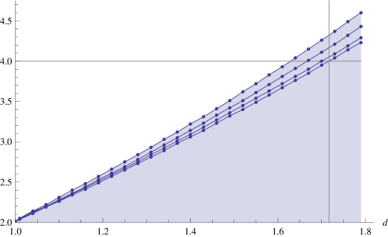
Figure 1: Restriction of the smallest scaling dimension of a spin $0$ operator in the $[N-1,N-1,1,1]$ representation of $SU(N)$ with $N=12$. The horizontal axis is the scaling dimension of the spin $0$ adjoint operator $\phi_{i}^{\bar{k}}$, $d=\Delta_{\phi_{i}^{\bar{k}}}$, and the vertical axis is the scaling dimension of the operator in the $[N-1,N-1,1,1]$ representation. Boundary curves are obtained by setting, from left to right, $(\texttt{derivativeOrder}=N_{\text{max}},\texttt{keptPoleOrder},\texttt{Lmax})=(10,14,24)$, $(12,14,24)$, $(14,16,24)$, and $(16,20,24)$, respectively. We see that the operator becomes relevant, i.e., the scaling dimension becomes smaller than $4$, when $d=\Delta_{\phi_{i}^{\bar{k}}}<1.71$.

Figure 1 is our result obtained by the above procedure. The horizontal axis is the scaling dimension of the spin $0$ adjoint operator $\phi_{i}^{\bar{k}}$, $d=\Delta_{\phi_{i}^{\bar{k}}}$. The shaded region is the smallest scaling dimension of a spin $0$ operator in the $[N-1,N-1,1,1]$ representation of $SU(N)$ with $N=12$ in a unitary conformal field theory. We stress again that to have a unitary conformal field theory, there must exist at least one spin $0$ operator in the $[N-1,N-1,1,1]$ representation in the shaded region. In particular, we see that, when $d=\Delta_{\phi_{i}^{\bar{k}}}<1.71$, there exists a spin $0$ relevant (i.e., its scaling dimension is smaller than $4$) operator in the $[N-1,N-1,1,1]$ representation. This leads to our upper bound on the mass anomalous dimension, Eq. (1.1), as explained in Sect. 1.

A similar analysis can be repeated by paying attention to the representation $[N-2,2]$ in Eqs. (2.3) and (2.25). Figure 2 is the restriction on the smallest scaling dimension of a spin $0$ operator in the $[N-2,2]$ representation of $SU(N)$ with $N=12$. This is obtained by the above numerical conformal bootstrap, by simply exchanging the role of $[N-1,N-1,1,1]$ and that of $[N-2,2]$. We see that there exists a spin $0$ relevant operator in the $[N-2,2]$ representation when $d=\Delta_{\phi_{i}^{\bar{k}}}<1.41$. This leads, by repeating the argument in Sect. 1, to an upper bound on the mass anomalous dimension, $\gamma_{m}^{*}\leq 1.59$. This is, however, weaker than the one following from the $[N-1,N-1,1,1]$ representation, Eq. (1.1).

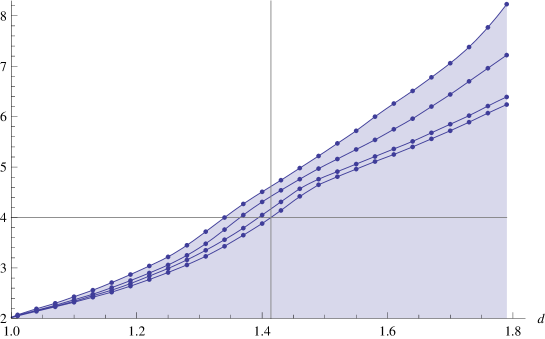
Figure 2: Restriction on the smallest scaling dimension of a spin $0$ operator in the $[N-2,2]$ representation of $SU(N)$ with $N=12$. The horizontal axis is the scaling dimension of the spin $0$ adjoint operator $\phi_{i}^{\bar{k}}$, $d=\Delta_{\phi_{i}^{\bar{k}}}$, and the vertical axis is the scaling dimension of the operator in the $[N-2,2]$ representation. Boundary curves are obtained by setting, from left to right, $(\texttt{derivativeOrder}=N_{\text{max}},\texttt{keptPoleOrder},\texttt{Lmax})=(10,14,24)$, $(12,14,24)$, $(14,16,24)$, and $(16,20,26)$, respectively. We see that the operator becomes relevant when $d=\Delta_{\phi_{i}^{\bar{k}}}<1.41$.

Although our analysis on the representation $[N-2,2]$ does not provide a useful upper bound on $\gamma_{m}^{*}$, quite interestingly, we see a kink-like behavior in the boundary curves in Fig. 2 around $d=\Delta_{\phi_{i}^{\bar{k}}}\sim 1.5$. Recalling the fact that in the numerical conformal bootstrap quite often one finds a known conformal field theory at a kink point on the boundary curve, the behavior in Fig. 2 is quite suggestive. It would be interesting to study this kink-like behavior in more detail and seek a possible conformal field theory with a global $SU(12)$ symmetry that corresponds to the (possible) kink in Fig. 2.

Among other representations in Eqs. (2.3) and (2.25), $[N-2,1,1]$ and its conjugate possess only odd spin operators, and spin $0$ operators which can correspond to a term in the action are not included. The representations $[N-1,1]$ and $1$ are somewhat special because, depending on the underlying field theory (e.g., $12$-flavor QCD), by using the flavored chiral rotation it is possible to construct spin $0$ operators in these representations whose scaling dimension is degenerate with $d=\Delta_{\phi_{i}^{\bar{k}}}$. For such a case, to draw a non-trivial conclusion one has to consider the second operator in these representations that has the scaling dimension greater than or equal to $d$. Although we carried out such an analysis for the representations $[N-1,1]$ and $1$, we do not present those results here, because the conclusion on the mass anomalous dimension seems quite dependent on the detail of the underlying theory.

Appendix A Upper bound on $\gamma_{m}^{*}$ for $N=8$ and $N=16$

Our crossing relation (2.25) holds for any $N\geq 3$ and, in this appendix, we present our numerical results for $N=8$ and $N=16$. These cases are also of great interest from perspective of the many-flavor QCD; it is conceivable that the $SU(3)$ gauge theory with $16$ fundamental massless fermions is a conformal field theory in the low-energy limit, while whether $8$-flavor QCD is conformal or not seems not yet quite conclusive; both systems can be simulated by using the staggered fermion. As for the $N=12$ case in the main text, we assume the absence of the spin $0$ relevant operator in the representation $[N-1,N-1,1,1]$ and derive the bound.

Figure 3 is our result on the smallest scaling dimension of a spin $0$ operator in the $[N-1,N-1,1,1]$ representation of $SU(N)$ with $N=8$, $N=12$, and $N=16$ (from left to right). Boundary curves are obtained by setting $(\texttt{derivativeOrder}=N_{\text{max}},\texttt{keptPoleOrder},\texttt{Lmax})=(14,16,24)$. As for $N=12$ in the main text, we see that when $d<1.67$ for $N=8$, and when $d<1.71$ for $N=16$, there emerges an $SU(N)$-breaking relevant operator in the system. Thus, by assuming the absence of such an operator, we have an upper bound on the mass anomalous dimension as

$$\gamma_{m}^{*}\leq 1.33\qquad\text{for $N=8$},$$ (A.1)

and

$$\gamma_{m}^{*}\leq 1.29\qquad\text{for $N=16$}.$$ (A.2)

Although the latter bound is numerically the same as Eq. (1.1), which is for $N=12$, there is no contradiction because here we are using a somewhat narrower search space for the linear operator $\Lambda$ ($N_{\text{max}}=14$) than that in the main text ($N_{\text{max}}=16$); the bound on $\gamma_{m}^{*}$ here is thus somewhat weaker than would be obtained from the setting in the main text.

Figure 3: Restriction on the smallest scaling dimension of a spin $0$ operator in the $[N-1,N-1,1,1]$ representation of $SU(N)$ with $N=8$, $N=12$, and $N=16$ (from left to right). The horizontal axis is the scaling dimension of the spin $0$ adjoint operator $\phi_{i}^{\bar{k}}$, $d=\Delta_{\phi_{i}^{\bar{k}}}$, and the vertical axis is the scaling dimension of the operator in the $[N-1,N-1,1,1]$ representation. We see that the operator becomes relevant when $d<1.67$ for $N=8$, and when $d<1.71$ for $N=16$.

Figure 4 is our result on the smallest scaling dimension of a spin $0$ operator in the $[N-2,2]$ representation of $SU(N)$ with $N=8$, $N=12$, and $N=16$ (from left to right). The parameters $(\texttt{derivativeOrder}=N_{\text{max}},\texttt{keptPoleOrder},\texttt{Lmax})$ are the same as above. As for the $N=12$ case in the main text, although the consideration of the operator in the $[N-2,2]$ representation does not provide a useful bound on $\gamma_{m}^{*}$, we also observe a kink-like behavior for $N=8$ and $N=16$. Again, it would be interesting to study this kink-like behavior in more detail and seek a possible conformal field theory that corresponds to these (possible) kinks.

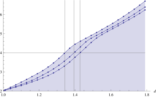
Figure 4: Restriction on the smallest scaling dimension of a spin $0$ operator in the $[N-2,2]$ representation of $SU(N)$ with $N=8$, $N=12$, and $N=16$ (from left to right). The horizontal axis is the scaling dimension of the spin $0$ adjoint operator $\phi_{i}^{\bar{k}}$, $d=\Delta_{\phi_{i}^{\bar{k}}}$, and the vertical axis is the scaling dimension of the operator in the $[N-2,2]$ representation. We see that the operator becomes relevant when $d<1.34$ for $N=8$, and when $d<1.42$ for $N=16$.

References

• (1) T. Banks and A. Zaks, Nucl. Phys. B 196, 189 (1982). doi:10.1016/0550-3213(82)90035-9
• (2) B. Holdom, Phys. Rev. D 24, 1441 (1981). doi:10.1103/PhysRevD.24.1441
• (3) B. Holdom, Phys. Lett. B 150, 301 (1985). doi:10.1016/0370-2693(85)91015-9
• (4) K. Yamawaki, M. Bando and K. i. Matumoto, Phys. Rev. Lett.  56, 1335 (1986). doi:10.1103/PhysRevLett.56.1335
• (5) T. W. Appelquist, D. Karabali and L. C. R. Wijewardhana, Phys. Rev. Lett.  57, 957 (1986). doi:10.1103/PhysRevLett.57.957
• (6) T. Appelquist and L. C. R. Wijewardhana, Phys. Rev. D 35, 774 (1987). doi:10.1103/PhysRevD.35.774
• (7) T. Appelquist and L. C. R. Wijewardhana, Phys. Rev. D 36, 568 (1987). doi:10.1103/PhysRevD.36.568
• (8) T. Appelquist, G. T. Fleming and E. T. Neil, Phys. Rev. Lett.  100, 171607 (2008) [Phys. Rev. Lett.  102, 149902 (2009)] doi:10.1103/PhysRevLett.100.171607 [arXiv:0712.0609 [hep-ph]].
• (9) J. Giedt, arXiv:1512.09330 [hep-lat].
• (10) R. C. Brower, G. Fleming, A. Gasbarro, T. Raben, C. I. Tan and E. Weinberg, arXiv:1601.01367 [hep-lat].
• (11) K.-I. Ishikawa, Y. Iwasaki, Y. Nakayama and T. Yoshie, Phys. Rev. D 87, no. 7, 071503 (2013) doi:10.1103/PhysRevD.87.071503 [arXiv:1301.4785 [hep-lat]].
• (12) E. Itou, PTEP 2015, no. 4, 043B08 (2015) doi:10.1093/ptep/ptv045 [arXiv:1307.6645 [hep-lat]].
• (13) R. Rattazzi, V. S. Rychkov, E. Tonni and A. Vichi, JHEP 0812, 031 (2008) doi:10.1088/1126-6708/2008/12/031 [arXiv:0807.0004 [hep-th]].
• (14) V. S. Rychkov and A. Vichi, Phys. Rev. D 80, 045006 (2009) doi:10.1103/PhysRevD.80.045006 [arXiv:0905.2211 [hep-th]].
• (15) D. Poland and D. Simmons-Duffin, JHEP 1105, 017 (2011) doi:10.1007/JHEP05(2011)017 [arXiv:1009.2087 [hep-th]].
• (16) R. Rattazzi, S. Rychkov and A. Vichi, Phys. Rev. D 83, 046011 (2011) doi:10.1103/PhysRevD.83.046011 [arXiv:1009.2725 [hep-th]].
• (17) R. Rattazzi, S. Rychkov and A. Vichi, J. Phys. A 44, 035402 (2011) doi:10.1088/1751-8113/44/3/035402 [arXiv:1009.5985 [hep-th]].
• (18) D. Poland, D. Simmons-Duffin and A. Vichi, JHEP 1205, 110 (2012) doi:10.1007/JHEP05(2012)110 [arXiv:1109.5176 [hep-th]].
• (19) S. El-Showk, M. F. Paulos, D. Poland, S. Rychkov, D. Simmons-Duffin and A. Vichi, Phys. Rev. D 86, 025022 (2012) doi:10.1103/PhysRevD.86.025022 [arXiv:1203.6064 [hep-th]].
• (20) P. Liendo, L. Rastelli and B. C. van Rees, JHEP 1307, 113 (2013) doi:10.1007/JHEP07(2013)113 [arXiv:1210.4258 [hep-th]].
• (21) S. El-Showk and M. F. Paulos, Phys. Rev. Lett.  111, no. 24, 241601 (2013) doi:10.1103/PhysRevLett.111.241601 [arXiv:1211.2810 [hep-th]].
• (22) C. Beem, L. Rastelli and B. C. van Rees, Phys. Rev. Lett.  111, 071601 (2013) doi:10.1103/PhysRevLett.111.071601 [arXiv:1304.1803 [hep-th]].
• (23) F. Kos, D. Poland and D. Simmons-Duffin, JHEP 1406, 091 (2014) doi:10.1007/JHEP06(2014)091 [arXiv:1307.6856 [hep-th]].
• (24) S. El-Showk, M. Paulos, D. Poland, S. Rychkov, D. Simmons-Duffin and A. Vichi, Phys. Rev. Lett.  112, 141601 (2014) doi:10.1103/PhysRevLett.112.141601 [arXiv:1309.5089 [hep-th]].
• (25) M. Berkooz, R. Yacoby and A. Zait, JHEP 1408, 008 (2014) Erratum: [JHEP 1501, 132 (2015)] doi:10.1007/JHEP01(2015)132, 10.1007/JHEP08(2014)008 [arXiv:1402.6068 [hep-th]].
• (26) S. El-Showk, M. F. Paulos, D. Poland, S. Rychkov, D. Simmons-Duffin and A. Vichi, J. Stat. Phys.  157, 869 (2014) doi:10.1007/s10955-014-1042-7 [arXiv:1403.4545 [hep-th]].
• (27) Y. Nakayama and T. Ohtsuki, Phys. Rev. D 89, no. 12, 126009 (2014) doi:10.1103/PhysRevD.89.126009 [arXiv:1404.0489 [hep-th]].
• (28) Y. Nakayama and T. Ohtsuki, Phys. Lett. B 734, 193 (2014) doi:10.1016/j.physletb.2014.05.058 [arXiv:1404.5201 [hep-th]].
• (29) L. F. Alday and A. Bissi, JHEP 1502, 101 (2015) doi:10.1007/JHEP02(2015)101 [arXiv:1404.5864 [hep-th]].
• (30) S. M. Chester, J. Lee, S. S. Pufu and R. Yacoby, JHEP 1409, 143 (2014) doi:10.1007/JHEP09(2014)143 [arXiv:1406.4814 [hep-th]].
• (31) F. Kos, D. Poland and D. Simmons-Duffin, JHEP 1411, 109 (2014) doi:10.1007/JHEP11(2014)109 [arXiv:1406.4858 [hep-th]].
• (32) Y. Nakayama and T. Ohtsuki, Phys. Rev. D 91, no. 2, 021901 (2015) doi:10.1103/PhysRevD.91.021901 [arXiv:1407.6195 [hep-th]].
• (33) C. Beem, M. Lemos, P. Liendo, L. Rastelli and B. C. van Rees, arXiv:1412.7541 [hep-th].
• (34) S. M. Chester, S. S. Pufu and R. Yacoby, Phys. Rev. D 91, no. 8, 086014 (2015) doi:10.1103/PhysRevD.91.086014 [arXiv:1412.7746 [hep-th]].
• (35) D. Simmons-Duffin, JHEP 1506, 174 (2015) doi:10.1007/JHEP06(2015)174 [arXiv:1502.02033 [hep-th]].
• (36) F. Gliozzi, P. Liendo, M. Meineri and A. Rago, JHEP 1505, 036 (2015) doi:10.1007/JHEP05(2015)036 [arXiv:1502.07217 [hep-th]].
• (37) Y. Nakayama and T. Ohtsuki, arXiv:1602.07295 [cond-mat.str-el].
• (38) D. Simmons-Duffin, arXiv:1602.07982 [hep-th].
• (39) Z. Fodor et al., Phys. Lett. B 703, 348 (2011) doi:10.1016/j.physletb.2011.07.037 [arXiv:1104.3124 [hep-lat]].
• (40) T. Appelquist, G. T. Fleming, M. F. Lin, E. T. Neil and D. A. Schaich, Phys. Rev. D 84, 054501 (2011) doi:10.1103/PhysRevD.84.054501 [arXiv:1106.2148 [hep-lat]].
• (41) T. DeGrand, Phys. Rev. D 84, 116901 (2011) doi:10.1103/PhysRevD.84.116901 [arXiv:1109.1237 [hep-lat]].
• (42) A. Cheng, A. Hasenfratz and D. Schaich, Phys. Rev. D 85, 094509 (2012) doi:10.1103/PhysRevD.85.094509 [arXiv:1111.2317 [hep-lat]].
• (43) Y. Aoki et al., Phys. Rev. D 86, 054506 (2012) doi:10.1103/PhysRevD.86.059903, 10.1103/PhysRevD.86.054506 [arXiv:1207.3060 [hep-lat]].
• (44) A. Cheng, A. Hasenfratz, G. Petropoulos and D. Schaich, JHEP 1307, 061 (2013) doi:10.1007/JHEP07(2013)061 [arXiv:1301.1355 [hep-lat]].
• (45) A. Cheng, A. Hasenfratz, Y. Liu, G. Petropoulos and D. Schaich, Phys. Rev. D 90, no. 1, 014509 (2014) doi:10.1103/PhysRevD.90.014509 [arXiv:1401.0195 [hep-lat]].
• (46) M. P. Lombardo, K. Miura, T. J. N. da Silva and E. Pallante, JHEP 1412, 183 (2014) doi:10.1007/JHEP12(2014)183 [arXiv:1410.0298 [hep-lat]].
• (47) E. Itou and A. Tomiya, PoS LATTICE 2014, 252 (2014) [arXiv:1411.1155 [hep-lat]].
• (48) G. Mack, Commun. Math. Phys.  55, 1 (1977). doi:10.1007/BF01613145
• (49) L. Susskind, Phys. Rev. D 16, 3031 (1977). doi:10.1103/PhysRevD.16.3031
• (50) N. Kawamoto and J. Smit, Nucl. Phys. B 192, 100 (1981). doi:10.1016/0550-3213(81)90196-6
• (51) M. F. L. Golterman and J. Smit, Nucl. Phys. B 245, 61 (1984). doi:10.1016/0550-3213(84)90424-3
• (52) M. F. L. Golterman and J. Smit, Nucl. Phys. B 255, 328 (1985). doi:10.1016/0550-3213(85)90138-5
• (53) W. J. Lee and S. R. Sharpe, Phys. Rev. D 60, 114503 (1999) doi:10.1103/PhysRevD.60.114503 [hep-lat/9905023].
• (54) F. A. Dolan and H. Osborn, Nucl. Phys. B 678, 491 (2004) doi:10.1016/j.nuclphysb.2003.11.016 [hep-th/0309180].