Perspective: How good is DFT for water?

Abstract

Kohn-Sham density functional theory (DFT) has become established as an indispensable tool for investigating aqueous systems of all kinds, including those important in chemistry, surface science, biology and the earth sciences. Nevertheless, many widely used approximations for the exchange-correlation (XC) functional describe the properties of pure water systems with an accuracy that is not fully satisfactory. The explicit inclusion of dispersion interactions generally improves the description, but there remain large disagreements between the predictions of different dispersion-inclusive methods. We present here a review of DFT work on water clusters, ice structures and liquid water, with the aim of elucidating how the strengths and weaknesses of different XC approximations manifest themselves across this variety of water systems. Our review highlights the crucial role of dispersion in describing the delicate balance between compact and extended structures of many different water systems, including the liquid. By referring to a wide range of published work, we argue that the correct description of exchange-overlap interactions is also extremely important, so that the choice of semi-local or hybrid functional employed in dispersion-inclusive methods is crucial. The origins and consequences of beyond-2-body errors of approximate XC functionals are noted, and we also discuss the substantial differences between different representations of dispersion. We propose a simple numerical scoring system that rates the performance of different XC functionals in describing water systems, and we suggest possible future developments.

I Introduction

Water is an endlessly fascinating substance with many anomalous properties, of which its expansion on freezing and its density maximum at $4$ ^∘C are just two of the most famous. The fascination is only deepened by the apparent simplicity of the H₂O molecule itself. Because of its importance for life, for the Earth’s geology and climate, and for innumerable domestic and industrial processes, water in all its forms has been one of the most widely studied of all substances. From the theoretical viewpoint, it offers unrivaled opportunities to deepen our understanding of hydrogen bonding (H-bonding). A little over $20$ years ago, the first attempts were reported to derive and interpret the properties of liquid water from electronic-structure calculations based on density functional theory (DFT) laasonen1993a ; tuckerman1994a ; sprik1996a . This idea has proven immensely productive, and has been developed by many research groups, but the search for a fully satisfactory DFT description of water systems has been unexpectedly arduous, and is not yet complete. Our aim here is to review what has been learnt so far, and to assess the challenges that remain. An important feature of the review is that we aim to cover DFT work not only on the liquid, but also on clusters and ice structures.

The first ever DFT simulations of liquid water, pioneered by Parrinello, Car and co-workers laasonen1993a ; tuckerman1994a ; sprik1996a ; silvestrelli1997a ; silvestrelli1999a , followed a long history of water modeling based on force fields (see e.g. Refs. bernal1933a ; rowlinson1951a ; barker1969a ; rahman1971a ; berendsen1981a ; jorgensen1983a ). It was recognized over $80$ years ago that the bent shape of the H₂O molecule and the electronegativity of oxygen make electrostatic forces very important bernal1933a . The earliest force fields represented the Coulomb interactions in terms of point charges, with overlap repulsion and dispersion modeled by simple potentials, the molecules being assumed rigid and unpolarizable. Such elementary models can be remarkably successful for the ambient liquid guillot2002a ; abascal2005a , but their transferability is poor. The dipole moment of the H₂O molecule is known to increase by $40-50$ % from the gas phase to the ice and liquid phases coulson1966a ; batista1998a ; silvestrelli1999b ; badyal2000a , so that the neglect of polarizability is a serious limitation. A large research effort has been devoted to the development of accurate models that treat the molecules as polarizable and flexible dang1997a ; burnham2002a ; ren2003a ; habershon2011a ; wikfeldt2013a and include the weak intermolecular covalency that has often been thought significant isaacs1999a ; nilsson2005a ; glendening2005a ; cobar2012a . The most sophisticated of these models have the declared aim of describing all water systems, from clusters through ice structures to the liquid (see e.g. Refs. fanourgakis2008a ; babin2012a ). Reviews of the many force fields that have been proposed can be found elsewhere, e.g. Refs. guillot2002a ; vega2009a ; vega2011a .

By definition, close approximations to the true exchange-correlation (XC) functional of DFT would automatically deliver everything offered by force-fields and more. The search for such approximations for pure water systems is important for several reasons. DFT gives direct access to electronic charge distributions, which are important for the interpretation of experimental observables such as infra-red spectra sharma2005a ; zhang2011c , dielectric properties sharma2007a , x-ray scattering intensities krack2002a , surface potentials kathmann2011a , etc. It also provides a way of investigating water systems completely independent of force-fields, so that it gives the possibility of fruitful dialog between the approaches. Although our review is restricted to pure water systems, the development of improved XC approximations reviewed here is highly relevant to the DFT description of more general aqueous systems, including solutions and acid-base systems laasonen1994a ; tuckerman1995a ; tuckerman1995b ; white2000a ; naor2003a ; iftimie2006a ; iftimie2008a ; marx2006a ; marx2010a ; hassanali2013a ; hassanali2014a , as well as confined water coudert2006a ; cicero2008a ; munoz-santiburcio2013a and water adsorbed on surfaces lindan1998a ; carrasco2011a ; carrasco2012a ; sulpizi2012a ; cheng2010a ; wang2012b ; wood2013a . The crucial role of H-bonding in the cohesion of water systems pauling1935a ; stillinger1980a makes them an outstanding paradigm of this bonding mechanism, which is so widespread in many other molecular systems, including those important in biology jeffrey1997a . This means that the challenges to DFT to be described here for pure water systems will have a wide relevance.

The XC functionals known as generalized gradient approximations (GGAs) are among the most popular and successful for a great variety of condensed-matter systems, and they were used for the first DFT simulations of liquid water. Appropriately chosen GGAs were found to give quite satisfactory binding energies for the water dimer sim1992a ; laasonen1992a ; laasonen1993b ; santra2007a and the common form of ice hamann1997a ; feibelman2008a , and when used in molecular dynamics (MD) simulations gave a reasonable structure for the liquid laasonen1993a ; sprik1996a ; silvestrelli1999a . The early successes prompted a surge of interest in the use of GGA-based simulations to explore a wide range of important questions concerning water itself, such as H-bond dynamics, electronic properties, and the structure and diffusion of hydronium and hydroxyl ions. Simulations of this kind have also been very widely used to probe the solvation shells around a variety of ions and other neutral solutes in water. A review of DFT-based MD work both on pure water and on a wide range of aqueous systems can be found in Ref. hassanali2014a . The widespread use of DFT for simulating interfaces involving aqueous systems and water adsorbed on surfaces is also noteworthy (see e.g. Refs. lindan1998a ; michaelides2006a ; carrasco2011a ; carrasco2012a ; skulason2007a ; sulpizi2012a ). The new insights gained in these investigations would in many cases have been difficult or impossible to achieve with force-field methods, and the enormous value of DFT-based simulations of aqueous systems is beyond dispute.

Nevertheless, it became clear over $10$ years ago that the description of liquid water given by GGAs was not completely satisfactory asthagiri2003a ; grossman2004a ; schwegler2004a ; fernandez-serra2004a ; sit2005a . Fortuitous cancelation of errors in the earlier work had made the approximations seem more accurate than they really were grossman2004a ; kuo2004b ; vandevondele2005a . It was also discovered that GGA predictions of energy differences between extended and compact structures of some water systems, including larger clusters and ice, are qualitatively wrong santra2008a ; shields2008a ; dahlke2008a ; santra2011a . These discoveries stimulated a re-examination of XC approximations for pure water systems that continues to this day, and we shall try to decribe what has been learnt from this. An important outcome will be that dispersion is crucially important, and that some of the errors of GGAs come from their failure to describe dispersion correctly. It has been recognized for many years that H-bonding is the dominant mechanism of cohesion in water systems pauling1935a ; stillinger1980a . However, H-bonding is a complex phenomenon, which can be analyzed into electrostatic attraction, polarization, dispersion and partial covalency arunan2011a , though the relative contributions of these components in water remain controversial, depending significantly on definition cobar2012a . The contribution of partial covalency (often termed charge transfer), for example, has been particularly contentious isaacs1999a ; ghanty2000a ; romero2001a ; nilsson2005a . In addition, good XC functionals must correctly describe exchange-repulsion and monomer deformation. Our point of view here will be that all these energy components can be in error, and our review of the research will try to assess where the main errors lie. The evidence will indicate that dispersion is far from being the only culprit.

We will start by reviewing DFT work on the water monomer and water clusters. The DFT description of the monomer (Sec. II) is important for the electrostatic, polarization and monomer deformation parts of the energy, while the dimer (Sec. III) provides tests of H-bonding, where exchange-repulsion, dispersion and weak covalency also play a role. Energies of the dimer in non-H-bonding geometries may help in separating the covalency contribution. DFT work on clusters from the trimer to the pentamer (Sec. IV) gives further information about polarizability, while the isomers of the hexamer (Sec. V) and larger clusters (Sec. VI) help to separate dispersion and exchange repulsion. We shall see that the energetics of ice structures (Sec. VII) is vital in assessing the roles of these energy components. The lessons learnt up to this point form the background to our review of DFT work on the liquid (Sec. VIII). In the final Sec. IX, we draw together the evidence from all the water systems to assess the ability of current XC functionals to account for all the components of the energy. We summarize by proposing a simple scoring scheme, which assigns a numerical score to any given XC functional, based on the quality of its predictions for clusters and ice structures. The scheme may help to gauge the likely performance of the functional on the liquid. We should note at the outset that water is a vast subject, so that our review will inevitably be incomplete, as well as reflecting our own personal perspective. We provide in the Appendix a brief survey of the main XC approximations that will be relevant.

II The water monomer

Since electrostatic interactions are very important in all water systems, we need to know that available XC functionals reproduce the charge distribution of the free H₂O monomer, or at least its leading multipole moments. This will ensure the correctness of the so-called first-order electrostatic energy, i.e. the Coulomb interaction energy of an assembly of molecules when the monomer charge distributions are taken to be those of free monomers. In reality, the electric fields of the monomers distort each other’s charge distributions, so it is important that XC functionals reproduce the polarizabilities of the free monomers, and ideally this should mean the response of the dipole and higher multipole moments to dipolar and higher multipolar fields.

Almost all published DFT work on the charge distribution of the free H₂O monomer reports only the dipole moment $\mu$, though some information is available for the quadrupole moments. Only a limited number of GGAs appear to have been studied, but the BLYP becke1988a ; lee1988a and BP86 becke1988a ; perdew1986a functionals reproduce the benchmark value of $\mu$ to within $\sim 3$ %, and the hybrid functionals B3LYP becke1993a ; stephens1994a and PBE0 perdew1996b ; adamo1999a are even better than this adamo1999a ; calaminici1998a ; fantin2007a . The rather sparse results for the quadrupole moments indicate that these are also correct to within a few percent cohen1999a . So far as we are aware, DFT calculations have been reported only for the components of the dipolar polarizability, and there is general agreement that GGAs always overestimate them by $\sim 10$ % mcdowell1995a ; tozer1998a ; calaminici1998a ; adamo1999a ; cohen1999a ; vancaillie2000a . (The overestimation of molecular polarizabilities by GGAs is a general phenomenon, which arises from the underestimation of the energies of virtual Kohn-Sham states relative to those of occupied states, which in turn is related to the incorrect behavior of the Kohn-Sham potential in the asymptotic region far from the molecule tozer1998a ; tozer1998b .) Hybrid functionals do much better, with the average polarizability from B3LYP and PBE0 being in error by $\sim 2$ % and less than $1$ % respectively tozer1998a ; adamo1999a ; vancaillie2000a ; hammond2009a .

The water monomer is flexible, and a correct description of its deformation energetics is likely to be important, for two reasons. One is that, in water clusters and condensed phases, formation of a H-bond weakens and lengthens the OH bond of the donor, and these effects help to determine the strength of the H-bond. The other reason is that the spectrum of intramolecular vibrations is an important experimental diagnostic of H-bond formation, which it is desirable to reproduce in simulations.

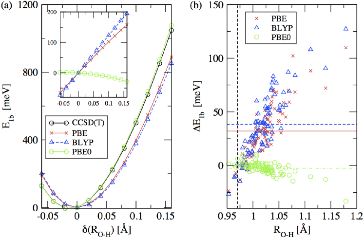
Figure 1: a) Variation of the monomer deformation energy $E_{\rm 1b}$ with deviation $\delta R_{\rm O-H}$ of the O-H bond length of an H₂O molecule from its equilibrium value in the symmetric stretch mode, calculated with CCSD(T), PBE, BLYP and PBE0. Inset shows the errors $\Delta E_{\rm 1b}$ of the deformation energy with the three XC functionals relative to CCSD(T) (benchmark minus DFT value of $E_{\rm 1b}$). (Note that $\delta R_{\rm O-H}$ is computed relative to the equilibrium value of the O-H bond length given by PBE, which is slightly greater than that calculated with PBE0 and CCSD(T).) (b) Errors $\Delta E_{\rm 1b}$ for deformed monomers drawn from a simulation of liquid water as a function of the longest O-H bond of each monomer. The vertical dashed line indicates the gas-phase equiibrium O-H bond length ($0.97$ Å) of a monomer (optimized with PBE) and the horizontal solid, dashed and dash-dotted lines represent the average errors of PBE, BLYP and PBE0 respectively. Note that a positive error $\Delta E_{\rm 1b}$ indicates that it is too easy to stretch O-H bonds of the monomers with a given XC functional compared with CCSD(T). Reproduced with permission from J. Chem. Phys. 131, 124509 (2009). Copyright 2009, American Institute of Physics.

The ability of GGA and hybrid functionals to describe monomer deformation was investigated by Santra et al. santra2009a , who showed that the energy cost of stretching the O-H bonds of the monomer is significantly underestimated by PBE and BLYP but is very accurately given by PBE0. This is shown in panel (a) of Fig. 1 which plots the deformation energy $E_{\rm 1b}$ in the symmetric mode as a function of the departure $\delta R_{\rm O-H}$ of the O-H bond length from its equilibrium value, $E_{\rm 1b}$ being computed with the PBE, BLYP and PBE0 approximations and with the benchmark CCSD(T) technique (coupled-cluster with single and double excitations and a perturbative treatment of triples helgaker2000a ). (We note that the small offsets of the minima of the plots of $E_{\rm 1b}$ vs $\delta R_{\rm O-H}$ are due to the fact that $\delta R_{\rm O-H}$ is computed in all cases relative to the equilibrium bond length given by PBE, which is slightly greater than the bond lengths given by PBE0 and CCSD(T).) The deviations of the GGA values of $E_{\rm 1b}$ from the benchmark values (inset of panel (a)) are ca. 100 meV for a bond stretch $\delta R_{\rm O-H}$ of $0.1$ Å, but the errors of PBE0 are much smaller. The authors examined the consequences of this for the liquid by drawing a large sample of monomers from an MD simulation of liquid water performed with flexible monomers. They found that bond stretches of up to ca. 0.1 Å are very common, and they confirmed the accuracy of PBE0 and the substantial underestimates of the deformation energy given by PBE and BLYP (see panel (b) of Fig. 1). This underestimate by GGAs, also noted by other authors xu2004b ; zhang2011b ; gillan2012a , correlates with an erroneous softening of the intramolecular OH stretch frequencies, which are underestimated by $\sim 3$ % and $\sim 4.2$ % with PBE and BLYP respectively, but are reproduced almost exactly by PBE0 santra2009a .

The comparisons for the monomer thus help us to assess the accuracy of XC functionals for three important parts of the energy in general water systems, namely first-order electrostatics, polarization and monomer deformation. For all three, GGAs appear to give reasonable, but far from perfect accuracy, while the accuracy of hybrid functionals is considerably better.

III Testing hydrogen-bonding: the dimer

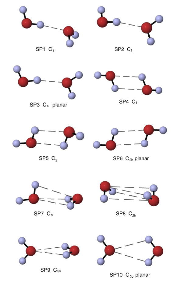
Figure 2: Geometries of the 10 Smith stationary points SP$n$ ($n=1,2,\ldots 10$) of the water dimer, with their point-group symmetries.

The dimer is the simplest water system we can use to test the accuracy of XC functionals for the energy of interaction between H₂O monomers in H-bonding and other geometries. The (H₂O)₂ system has been thoroughly studied by very accurate CCSD(T) calculations, which are believed to give the interaction energy in any geometry with errors relative to the exact value of no more than $\sim 5$ meV klopper2000a ; tschumper2002a . We know from such calculations that the geometry having the global minimum energy is the configuration labeled SP1 in Fig. 2. This is a typical H-bonding geometry, with the OH bond of the donor directed towards the O atom of the acceptor. We define the dimer binding energy $E_{\rm b}^{\rm dim}$ as twice the energy of an isolated equilibrium monomer minus the energy of the dimer in its global-minimum geometry. According to CCSD(T), $E_{\rm b}^{\rm dim}$ is $217.6\pm 2.0$ meV, the equilibrium O-O distance $R_{\rm OO}^{\rm dim}$ being $2.909$ Å tschumper2002a ; these values are consistent with the somewhat uncertain experimental values curtiss1979a ; odutola1980a ; mas2000a .

Acceptable DFT approximations must reproduce benchmarks for the binding energy $E_{\rm b}^{\rm dim}$ and the geometry of the global minimum, and in fact most DFT work on the water dimer has focused exclusively on this configuration. However, this is not enough, because both in the liquid and in compressed ice phases water monomers approach each other closely in non-H-bonded geometries, and the energetics of such geometries is very important. A simple way of going beyond the global minimum is to study the set of configurations on the energy surface of the dimer known as the Smith stationary points (Fig. 2) smith1990a , some of which resemble geometries found in dense ice structures. We also review here assessments of XC functionals made using large statistical samples of dimer geometries designed to be relevant to condensed phases.

We discuss first local and semi-local XC functionals, including the local density approximation (LDA kohn1965a ; ceperley1980a ; perdew1981a ), GGAs of different kinds, and hybrids, confining ourselves initially to the global minimum geometry. (See the Appendix for information about the relevant XC approximations.) Several extensive surveys have been published on the predictions of semi-local functionals for the water dimer santra2007a ; xu2004b ; dahlke2005a . In some work on the dimer, full basis-set convergence was not achieved, so that the accuracy of the functionals themselves was not completely clear. However, Ref. santra2007a reported calculations very close to the complete basis set (CBS) limit for 16 semi-local functionals applied to the dimer and other small water clusters. Table 1 reproduces some of the $E_{\rm b}^{\rm dim}$ and $R_{\rm OO}^{\rm dim}$ values from that work, supplemented with results from Ref. zhang2011a and from our own calculations performed in the present work. We performed our own calculations using the molpro molpro and vasp vasp codes, following the procedures described elsewhere alfe2014a . The wide spread of predicted binding energies is striking. The LDA is clearly unacceptable, since it overbinds the dimer by nearly a factor of 2 lee1994a ; lee1995a , and there are other functionals, such as PBEsol perdew2008a , which also overbind significantly. At the other extreme, functionals such as BLYP and revPBE zhang1998a underbind quite seriously. Among the best functionals for $E_{\rm b}^{\rm dim}$ are PBE and its hybrid version PBE0. It will become clear below that functionals predicting a good $E_{\rm b}^{\rm dim}$ can still give a poor description of larger clusters, ice structures and liquid water. The wide variability of $E_{\rm b}^{\rm dim}$ with different semi-local functionals will turn out to be crucial for the understanding of extended water systems.

The reason why different semi-local functionals give such different binding energies in dimers of small molecules such as water is well known. It was recognized long ago harris1985a that the gross overbinding given by LDA arises from a spurious exchange attraction. In GGAs, this spurious attraction is suppressed by the exchange-enhancement factor $F_{\rm X}(s)$, which depends on the reduced gradient $x=|\nabla\rho|/\rho^{4/3}$ of the electron density $\rho$ through the quantity $s=x/(2(3\pi^{2})^{1/3})$. Roughly speaking, the exchange-overlap interactions of BLYP and revPBE are strongly repulsive and those of PBE and PW91 are weakly repulsive because of the very different behavior of their $F_{\rm X}(s)$ factors in the region of large $s$ where the tails of the monomer densities overlap lacks1993a ; zhang1997a ; wu2001a ; kannemann2009a ; murray2009a ; kanai2009a . This important difference between GGAs will be referred to again several times.

Dispersion plays a vital role in the energetics of water systems, as we shall see later, but is not correctly described by the semi-local functionals discussed above. The past 20 years have seen the introduction of several different ways of accounting for dispersion (see the Appendix, and recent reviews klimes2012a ; dilabio2014a ). One approach consists of the addition of potentials of various kinds to existing functionals, first explored nearly 20 years ago (see e.g. Refs. meijer1996a ; gianturco2000a ; wu2001a ) and then extensively developed by Grimme grimme2004a ; grimme2006a ; grimme2010a , Tkatchenko and Scheffler (TS) tkatchenko2009a and others. An alternative is the incorporation of explicitly non-local correlation functionals, pioneered by Lundqvist, Langreth and others dion2004a ; klimes2010a ; vydrov2010a . The DCACP method of Rothlisberger and co-workers vonlilienfeld2004a and the closely related DCP method of Ref. torres2012a are also noteworthy. In all these methods, a representation of non-local correlation energy is added to a chosen semi-local functional. The naming of these different approaches is not completely uniform in the literature, so we summarize briefly the nomenclature used throughout this review. The approach now generally known as the Grimme method comes in three versions, which we denote by func-D1, func-D2 and func-D3, where “func” is the name of the semi-local or hybrid functional to which dispersion is added. Similarly, we denote TS methods by func-TS, and methods based on the non-local functional of Ref. dion2004a by func-DRSLL (the acronym DRSLL stands for the authors of Ref. dion2004a ). We denote by rPW86-DF2 the method of Ref. lee2010a (sometimes known as LMKLL after the authors of this Ref.), which employs a modified form of the DRSLL non-local correlation functional added to a revised version of the PW86 semi-local functional perdew1986a .

We summarize in Table 1 the dimer binding energies $E_{\rm b}^{\rm dim}$ and equilibrium O-O distances predicted for the global minimum geometry by some of these schemes. This shows that the addition of dispersion to a semi-local functional always increases $E_{\rm b}^{\rm dim}$, as expected. For BLYP and revPBE, which significantly underestimate $E_{\rm b}^{\rm dim}$, the dispersion-inclusive versions BLYP-D3 and revPBE-DRSLL give improved values of $E_{\rm b}^{\rm dim}$, though the latter functional is still significantly underbound. By contrast, the addition of TS dispersion to PBE and PBE0, which already gave accurate values of $E_{\rm b}^{\rm dim}$, inevitably worsens the predictions. The DRSLL-type functionals are particularly instructive in this regard. Their original form dion2004a , based on revPBE, generally underbinds molecular dimers, so the underestimate of $E_{\rm b}^{\rm dim}$ for the H₂O dimer by revPBE-DRSLL comes as no surprise. It was pointed out  gulans2009a ; klimes2010a that better binding energies are obtained if less repulsive semi-local functionals are used in place of revPBE. It turns out that PBE is too weakly repulsive, so that PBE-DRSLL generally overbinds molecular dimers, including (H₂O)₂. However, if the exchange functional is appropriately tuned, much better approximations can be obtained. This is illustrated in the Table by the optPBE-DRSLL and optB88-DRSLL approximations, which are based on tuned forms of the PBE and B88 functionals. Similar arguments underlie the rPW86-DF2 non-local functional lee2010a . The comparisons shown in the Table indicate that the addition of dispersion increases $E_{\rm b}^{\rm dim}$ by up to $\sim 35$ meV. This is comparable with the variation of $E_{\rm b}^{\rm dim}$ resulting from different choices of semi-local or hybrid functional. We shall see in Sec. VIII that addition of dispersion to a semi-local functional can bring large changes in the structure and equilibrium density of the liquid, so that errors as large as $35$ meV in $E_{\rm b}^{\rm dim}$ are important.

We noted earlier the importance of accuracy for configurations other than the global minimum, and many authors have drawn attention to the role of non-H-bonded pair configurations in condensed phases of water wu2001a ; dahlke2005a ; ireta2004a ; lin2009a ; wang2011a ; zhang2011a . The Smith stationary points (Fig. 2) provide some relevant geometries, but the only systematic studies of DFT errors in these configurations appear to be those of Refs. gillan2012a ; anderson2006a . Anderson and Tschumper anderson2006a studied 10 different GGA and hybrid methods. All approximations gave the correct energy ordering, but most of them overestimated the energies relative to that of the global minimum, particularly for configurations SP4, SP5 and SP6, which closely resemble configurations in ice VIII. Relative energies for some semi-local and hybrid functionals are summarized in Table 2, which shows that PBE and BLYP both overestimate the relative energy of configuration SP6 by over $30$ meV. Hybrid approximations are appreciably better, but still overestimate the relative energies. Calculations of the energies relative to the global minimum with dispersion-inclusive methods do not appear to have been published, so we have made our own (see Table 2). We find that optPBE-DRSLL and rPW86-DF2 are both quite satisfactory, their errors in the relative energies all being less than $15$ meV. However, both PBE-TS and PBE0-TS are less satisfactory, giving relative energies of configurations 4, 5 and 6 in error by $\sim 30$ meV.

A characterization of XC errors for the global minimum and some special geometries is illuminating and useful, but a full characterization should cover all relevant O-O distances and monomer orientations. One way of doing this is to analyze the errors for large samples of dimers drawn from a MD simulation of the liquid, as has been done by Santra et al. santra2009a and Gillan et al. gillan2012a . For this purpose, we must separate 1-body and 2-body errors in the sense of the many-body expansion (MBE) hankins1970a ; xantheas1994a ; pedulla1998a , which will also be important later. In general, the total energy $E(1,2,\ldots N)$ of a system of $N$ monomers can be exactly expressed as:

$$E(1,2,\ldots N)=\sum_{i}E^{(1)}(i)+\frac{1}{2}{\sum_{i,j}}^{\prime}E^{(2)}(i,j)+\frac{1}{6}{\sum_{i,j,k}}^{\prime}E^{(3)}(i,j,k)+\ldots\;.$$ (1)

Here, $E^{(1)}(i)$ is the 1-body energy of monomer $i$ in free space, with the argument $i$ being short-hand for the set of coordinates specifying its geometry. Similarly, $E^{(2)}(i,j)$ is the 2-body energy of dimer $(i,j)$, i.e. its total energy minus the 1-body energies of monomers $i$ and $j$, with the arguments $i$ and $j$ being short-hand for the geometries of the monomers (the prime on the summation indicates the omission of terms $i=j$). The 3-body and higher terms needed for systems larger than the dimer are defined analogously. The zero of energy is conveniently taken as $N$ times the energy of an isolated equilibrium monomer. To analyze the errors of a chosen XC functional, the total energy of each dimer in the sample and the 1-body energies of its monomers are computed, and the 2-body energy is obtained by subtracting from the total dimer energy the sum of the two monomer energies. The 1- and 2-body errors are then obtained by subtracting benchmark values of the 1- and 2-body energies, typically computed with CCSD(T).

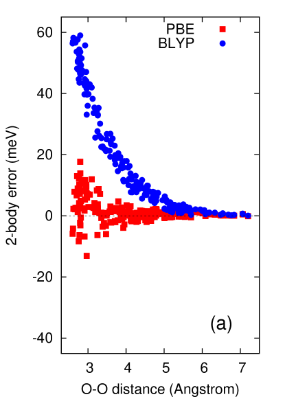
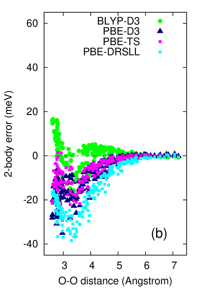
Figure 3: Errors of (a) semi-local functionals PBE and BLYP and (b) dispersion-inclusive functionals BLYP-D3, PBE-D3, PBE-TS and PBE-DRSLL for the 2-body energies of a sample of dimer geometries drawn from a MD simulation of liquid water gillan2012a .

Santra et al. santra2009a analyzed the errors of the BLYP, PBE and PBE0 functionals for dimers drawn from the liquid. BLYP values of the 2-body energies were underbound by an average of $\sim 40$ meV, while PBE and PBE0 values were overbound by $\sim 10$ meV. Interestingly, the errors of all three functionals showed a scatter of around $\pm 15$ meV about their averages at typical O-O nearest-neighbor distances of $\sim 2.8$ Å. There may be a link here with the errors in the relative energies of the Smith stationary points. An interesting finding from the same work santra2009a was that the known enhancement of H-bond energy by elongation of the donor OH bond is significantly exaggerated by both GGA functionals. The work of Ref. gillan2012a examined the 2-body errors computed with semi-local functionals for a thermal sample of dimers covering a range of O-O distances from $2.5$ to over $7.0$ Å. This revealed the expected systematic underbinding of BLYP over this range, and the much smaller errors of PBE, as illustrated in Fig. 3. We also present in this Figure calculations on the same thermal sample performed with the BLYP-D3, PBE-D3, PBE-TS and PBE-DRSLL functionals. We see that the excessive repulsion of BLYP is largely eliminated by BLYP-D3, which becomes slightly overbound between $3.0$ and $4.0$ Å. However, the PBE-based functionals are all overbound, with the overbinding errors of PBE-DRSLL being particularly strong in this range. Interestingly, the typical difference of 2-body energy between the BLYP and PBE functionals is comparable with the shifts due to dispersion, so that addition of D3 dispersion to BLYP brings its 2-body energy rather close to that of uncorrected PBE. The typical energy difference between the dispersion-corrected functionals BLYP-D3 and PBE-DRSLL is on the same scale as the energy shifts due to dispersion, so that the robustness of the methods clearly needs discussion. It is notable that the substantive differences between the various PBE-based methods in the region $3.0-4.0$ Å exist despite the close agreement between their global-minimum binding energies (Table 1).

It has been shown by Bartók et al. bartok2013a that machine-learning techniques operating on very large thermal samples of dimers can be used to create very accurate, but rapidly computable representations of the 1- and 2-body errors of chosen XC functionals. These techniques, based on the GAP (Gaussian approximation potential) method of machine learning bartok2010a , give a way of compensating almost exactly for the 1- and 2-body errors of any chosen XC functional. We review below (Secs. VI and VII) work on large water clusters and ice based on XC functionals corrected in this way.

In summary, we have seen that both semi-local and dispersion-inclusive functionals vary quite widely in their predictions of the H-bond energy. The variability affects the 2-body energy in the important region of O-O separation extending from $2.5$ to at least $4.0$ Å. We have noted the importance of the exchange-enhancement factor as one cause of this variability. The variation between different functionals is comparable with the increase of binding energy resulting from the addition of dispersion. The energies of the Smith stationary points relative to the global minimum are significantly overestimated by both semi-local and dispersion-inclusive functionals.

IV Cooperative hydrogen-bonding in small clusters

It has long been known that hydrogen bonding in water and in many other molecular systems is a cooperative effect: if molecule A donates a H-bond to molecule B, the propensity of molecule B to donate a H-bond to molecule C is thereby enhanced frank1957a ; elrod1994a ; jeffrey1997a ; karpfen2002a ; xu2002a . The cooperativity manifests itself in the non-additivity of H-bond energies. In suitable geometries, an assembly of water molecules is stabilized by the mutual enhancement of H-bonds hankins1970a ; white1990a ; xantheas1994a ; xantheas2000a , so that the overall binding energy is greater than the sum of dimer binding energies. This non-additivity of binding energies can be understood as resulting from molecular polarizability: the electron cloud on each monomer is distorted by the electric fields of its neighbors, and this changes its electrostatic interaction with other monomers. We noted in the Introduction that this is a strong effect, since molecular polarizability enhances the dipole moment of water monomers in ice and liquid water by $40-50$ % above that of monomers in free space coulson1966a ; batista1998a ; silvestrelli1999a ; badyal2000a . It was suggested by Frank and Wen frank1957a that the cooperativity would play an important role in the dynamical making and breaking of H-bonds in liquid water, and subsequent calculations and experiments have fully confirmed the importance of H-bond cooperativity in water systems of all kinds, including ice and clusters (see e.g. Ref. luck1998a ). It is clearly important to know whether DFT approximations reproduce these cooperative effects.

Fortunately, H-bond cooperativity is already important in small water clusters, where it has been extensively studied both experimentally and theoretically xantheas1993a ; saykally1993a ; xantheas1994a ; liu1996b ; gregory1996a ; xantheas2000a ; keutsch2003a ; glendening2005a ; santra2007a ; bryantsev2009a ; cobar2012a ; neela2010a ; guevara-vela2013a . These systems provide a simple way of testing the accuracy of DFT approximations in describing non-additivity, since very accurate benchmarks are readily available. We discuss here the trimer, tetramer and pentamer, leaving till Sec. V the hexamer, which raises issues beyond H-bond cooperativity. Experiments and accurate quantum chemistry calculations show that the most stable configurations of the (H₂O)_n clusters with $n=3$, $4$ and $5$ are quasi-planar and cyclic xantheas1993a ; xantheas1994a ; liu1996b ; xantheas2000a . An important indication of the progressive strengthening of the H-bonds is that the O-O distance shortens from $\sim 2.91$ Å in the dimer to $2.72$ Å in the pentamer liu1996b ; santra2007a . Another commonly used measure for the strength of a H-bond is the red-shift of the intramolecular stretching frequency of the donor O-H bond. Theory and experiment both find an increasing red-shift on passing from the trimer to the pentamer buck2000a .

For reference data on the non-additivity of the binding energies, we rely on benchmark MP2 and CCSD(T) calculations near the CBS limit, since accurate experimental data is not available. (MP2 is the second-order Møllet-Plesset approximation helgaker2000a , which is often nearly as accurate as CCSD(T) for water systems.) The non-additivity can be quantified using the many-body expansion (MBE) introduced above in eqn (1). The non-additive parts of the energy are characterized by the 3-body and higher-body terms $E^{(n)}$. For a small cluster (H₂O)_n in a given geometry, it is straightforward to compute benchmark total energies of all the monomers, dimer, trimers, etc. that can be formed from the cluster, and from these the terms $E^{(1)}(i)$, $E^{(2)}(i,j)$, $E^{(3)}(i,j,k)$ etc. of the MBE can be extracted. It has been shown by Xantheas xantheas2000a that the 3-body and higher components of the energy play a vital role in determining the relative energies of different conformations of the water trimer, tetramer and pentamer.

The performance of a wide variety of semi-local and hybrid XC functionals on the binding energies of the water trimer, tetramer and pentamer in their most stable geometries has been assessed by Santra et al. santra2007a . MP2 energies near the CBS limit were used as reference, the evidence being that these energies should differ from CCSD(T) values by no more than a few meV per H-bond. The functionals studied included the popular GGAs PBE, PW91 and BLYP and some less common ones such as XLYP, PBE1W, mPWLYP and BP86, the hybrid functionals PBE0, B3LYP and X3LYP, and the meta-GGA functional TPSS (references to the definitions of these functionals can be found in Ref. santra2007a ). As expected from their performance on the dimer, BLYP was found to be always quite strongly underbound, and PBE and PW91 always overbound. The B3LYP functional was a considerable improvement on BLYP, while the hybrids PBE0 and X3LYP gave almost perfect binding energies. The TPSS meta-GGA turned out to be somewhat worse than its parent functional PBE.

For present purposes, the most important finding of Ref. santra2007a is that all the functionals reproduce semi-quantitatively the cooperative enhancement of the H-bond energies given by the MP2 benchmarks. According to the benchmarks, the binding energy per H-bond is enhanced by a modest $6$ % in the trimer, increasing to a more impressive $46$ % in the pentamer. With very few exceptions, all the functionals give enhancements between $4$ and $8$ % in the trimer and between $45$ and $55$ % in the pentamer. Notably, the enhancement is overestimated by almost all the functionals in the tetramer and pentamer, perhaps because most functionals overestimate the polarizability of the water monomer (see Sec. II). It is also noted in Ref. santra2007a that for all the functionals the error in the binding energy per H-bond is almost independent of cluster size, though the error becomes more positive (more strongly bound) for some functionals, including PBE. This suggests that for a given DFT functional its error in the H-bond energy of the dimer is likely to be a good guide to its error in the H-bond energy in larger water aggregates. The authors also note that the known shortening of the equilibrium O-O distance with increasing cluster size is also semi-quantitatively reproduced by all the functionals.

To summarize, the work on small clusters up to the pentamer shows that H-bond cooperativity becomes a strong effect as we go to larger aggregates, but most XC functionals appear to describe the non-additivity of energies fairly accurately. Semi-local functionals generally overestimate the enhancement of H-bond strength, but hybrid functionals do better than GGAs.

V Compact versus extended geometries: the hexamer

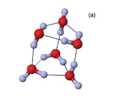
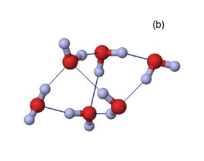
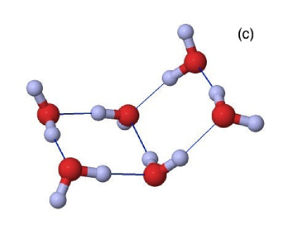
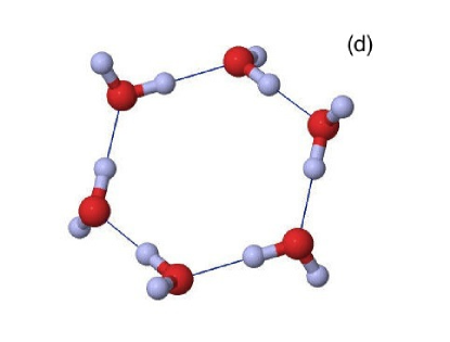
Figure 4: Isomers of the water hexamer: (a) prism, (b) cage, (c) book and (d) ring.

The hexamer occupies a special place in water studies, because it is the smallest cluster for which three-dimensional structures compete energetically with the two-dimensional cyclic structures just discussed for the trimer, tetramer and pentamer. There are many local minima on its complex energy surface tsai1993a ; kryachko1999a ; hincapie2010a , but here we pay particular attention to four of them, known as the prism, the cage, the book and the ring (Fig. 4). In the ring, each monomer is H-bonded to two neighbors, and all six H-bonds are of canonical form, with the donor O-H bond pointing directly at the acceptor O atom. In the prism, by contrast, each monomer is 3-fold coordinated, but the nine H-bonds are strongly distorted. In their coordination and H-bond count, the cage resembles the prism and the book resembles the ring. Are the extended ring and book structures with fewer but stronger H-bonds more or less stable than the compact cage and prism with more but weaker bonds? This is an important question, because the competition between compact and extended structures is central to the energetics of solid and liquid water phases.

In fact, CCSD(T) calculations close to the CBS limit leave no doubt that the energy ordering from lowest to highest is prism $<$ cage $<$ book $<$ ring gillan2012a ; olson2007a ; dahlke2008a ; bates2009a ; wang2010a . This ordering is confirmed by diffusion Monte Carlo (DMC) calculations foulkes2001a ; needs2010a , which give total binding energies relative to free monomers and total energy differences between the isomers in accord with CCSD(T) to within $\sim 5$ meV/monomer santra2008a . The fact that the compact prism and cage are more stable than extended structures such as the ring was already suggested by early MP2 calculations tsai1993a ; pedulla1998a ; xantheas2002a . It is now established that MP2 in the CBS limit gives the same stability ordering as CCSD(T) for the prism, cage, book and ring, though MP2 underestimates the difference of total binding energy of the ring and prism by $\sim 25$ meV olson2007a ; santra2008a ; dahlke2008a ; bates2009a . The prism and cage isomers are very close in energy, but CCSD(T) makes the prism more stable by $\sim 10$ meV bates2009a . (We note that this statement refers to energy-minimized structures; in the real world, zero-point and thermal vibrational energies appear to be large enough to reverse the stabilities of these two isomers liu1996a ; wang2012a .)

Several detailed studies have investigated the accuracy of DFT approximations for the relative energies of the different isomers and also for their overall binding energies with respect to free monomers. Between them, these studies cover a wide variety of methods. The works of Dahlke et al. dahlke2008a and Santra et al. santra2008a investigated respectively 11 and 12 different functionals, including GGAs, meta-GGAs, hybrids and hybrid-meta-GGAs. Later studies gillan2012a ; wang2010a ; gillan2014a ; pruitt2013a covered a range of GGAs and hybrids, and Ref. pruitt2013a studied a number of dispersion-inclusive methods. The remarkable outcome of these studies is that almost all the semi-local approximations erroneously make the ring or book more stable than the prism and cage. The only exceptions reported in these papers are the three Minnesota functionals M06-L, M05-2X and M06-2X dahlke2008a . On the positive side, a number of commonly used functionals (e.g. PBE, PBE0) give quite accurate values for the average binding energies of the four isomers, though others (e.g. BLYP, revPBE) are seriously underbound. The problems of semi-local XC functionals are illustrated in Table 3, where we compare their predicted binding energies with the CCSD(T) and DMC benchmarks.

The semi-local functionals just referred to do not explicitly describe dispersion, and it is natural to assume that this is the main cause of the erroneous stability ordering of the hexamers. This makes physical sense, because compact structures will be more strongly stabilized than extended structures by a pairwise attraction. The importance of dispersion has been confirmed by several studies of the hexamer santra2008a ; kelkkanen2009a ; silvestrelli2009a , showing that different dispersion-inclusive DFT methods all correct the wrong stability ordering and bring the relative energies of the isomers into respectable agreement with the benchmarks, as can be seen from the illustrative examples given in Table 3.

In spite of this compelling evidence, there are clear indications that dispersion is not the only source of errors in the XC functionals. These indications come from the many-body analyses reported in several papers. We saw in previous Sections how the binding energies of clusters can be separated into their 1-body, 2-body, and beyond-2-body components. The same approach can be applied to the errors of XC functionals, i.e. the deviations of approximate DFT energies from benchmarks. If the errors of XC approximations for the hexamer were entirely due to poor dispersion, we would expect them to be mainly 2-body errors, because beyond-2-body dispersion is generally much less significant than 2-body dispersion in water systems. (See e.g. Ref. vonlilienfeld2010a , which indicates that 3-body dispersion contributes ca. 100 times less than 2-body dispersion to the cohesive energy of ice Ih.) However, the reality is more complex. For the energy differences between the isomers, the errors of the BLYP and revPBE approximations are indeed mainly 2-body errors, but it turns out that the errors of PW91, PBE and PBE0 are largely beyond-2-body errors wang2010a ; gillan2012a ; gillan2013a ; gillan2014a . The importance of beyond-2-body errors in the energetics of the hexamer has been noted in Ref. pruitt2013a . On the other hand, the average binding energy of the four isomers is quite accurately given by PBE and PBE0 (see above), which reproduce both its 2-body and beyond-2-body components. (By “average binding energy” we mean the sum of the binding energies of the four isomers divided by 4.) However, the large error in the average binding energy given by BLYP arises from its excessive 2-body repulsion together with a smaller but still significant beyond-2-body overbinding gillan2012a ; gillan2013a . These facts indicate that the errors cannot be explained by incorrect dispersion alone.

It has been proposed recently gillan2014a that the many-body errors of GGAs for water (and other molecular systems) are closely linked to the choice of exchange-enhancement factor $F_{\rm X}$, which we know has an important influence on the 2-body interaction energy (see Sec. III). It appears that an $F_{\rm X}$ that gives excessive exchange-overlap repulsion in the dimer also tends to produce an overly attractive 3-body interaction, while an $F_{\rm X}$ whose 2-body exchange-overlap repulsion is too weak produces a spurious 3-body repulsion. The suggestion is that the accurate dimer binding energy given by PBE results from an overly weak exchange-repulsion mimicking the missing dispersion, the indirect consequence being the erroneous stability ordering in the hexamer due to the exaggerated 3-body repulsion. Conversely, the excessive 2-body repulsion of BLYP, to which dispersion should be added, is linked to the unduly attractive 3-body interaction noted above. The idea of an inverse correlation between the 2-body and beyond-2-body errors of semi-local functionals is confirmed by recent work on a wide range of molecular trimers rezac2015a .

The extensive work on the hexamer teaches us several lessons. First, good accuracy for the dimer (and other clusters smaller than the hexamer) is no guarantee of even qualitative correctness for the relative stability of compact and extended conformations. Second, many-body errors may be at least as important as 2-body errors, but the relative importance of the two kinds of error depends strongly on the exchange-correlation functional. Third, dispersion is crucial, and demands to be correctly described. Fourth, dispersion is not the only source of errors, and there is evidence that the many-body errors are associated with exchange. We shall see in the following how these lessons are reinforced by DFT work on larger clusters, ice structures and the liquid.

VI Larger clusters

For many years, quantum-chemistry benchmark calculations were feasible only on rather small clusters, with the hexamer representing the practical limit for basis-set converged CCSD(T). However, technical innovations are now helping to extend the calculations to much larger clusters without significant loss of accuracy. In fact, well converged MP2 calculations were possible on clusters of 20 - 30 monomers several years ago, but with the development of linear-scaling methods, they can now be applied to even larger systems werner2003a ; doser2009a . Corrections for the difference between CCSD(T) and MP2 can then be made using the many-body expansion for this difference gora2011a . In addition, there is growing evidence that the accuracy of quantum Monte Carlo methods foulkes2001a ; needs2010a rivals that of CCSD(T) for non-covalent interactions gurtubay2007a ; ma2009a ; santra2011a ; gillan2012a ; dubecky2013a ; ambrosetti2014a , and the mild scaling of these methods with system size and their high efficiency on parallel computers make it practical to compute benchmarks for water systems containing $30$ or more monomers alfe2013a ; morales2014a .

The availability of very accurate benchmark energies for large clusters opens the interesting possibility of tracing out the development of DFT errors as a function of cluster size. The notion here is that as we go to ever larger clusters the errors should come to resemble ever more closely those seen in ice structures and the liquid. Furthermore, an analysis of the errors into their 2-body and beyond-2-body components, similar to that discussed above for the hexamer, allows us to deepen our understanding of the continuous connections between these errors in clusters and in condensed phases.

These ideas have been explored alfe2013a for thermal samples of water clusters containing up to $27$ monomers, the benchmark energies being computed with the DMC technique. The sets of configurations for each water cluster were drawn from MD simulations performed with a realistic force field that treats the monomers as flexible and polarizable. For large enough clusters, these configurations should be roughly typical of those found in small water droplets. The time-varying radius of a cluster of $N$ monomers can be characterized by the quantity $R_{\rm gyr}(t)$ defined by:

$$R_{\rm gyr}(t)^{2}=\frac{1}{N}\sum_{i=1}^{N}\left|{\bf r}_{i}(t)-\bar{\bf r}(t)\right|^{2}\;,$$ (2)

where ${\bf r}_{i}(t)$ is the position of the O atom of monomer $i$ at time $t$, and $\bar{\bf r}(t)$ is the centroid of these O positions. This “radius of gyration” $R_{\rm gyr}(t)$ fluctuates in time as the cluster spontaneously breathes in and out, exploring compact and extended configurations. We saw in Sec. V that the errors of GGAs for the hexamer grow more positive as we pass from extended to compact isomers, and one might expect a similar dependence on $R_{\rm gyr}$ for thermal clusters.

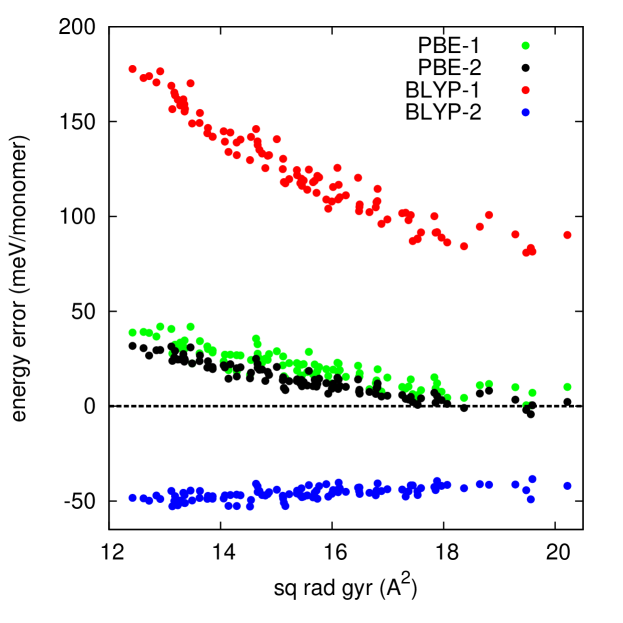
Figure 5: Errors in computed binding energy per monomer (meV units) of the water 27-mer as a function of radius of gyration (see text). Binding energies are computed with the PBE and BLYP functionals, corrected for 1- and 2-body errors, with benchmark values from diffusion Monte Carlo (DMC) calculations. Adapted with permission from J. Chem. Phys. 141, 014104 (2014) .

This expectation is amply fulfilled for the GGAs examined so far, namely BLYP and PBE. The analysis of the errors of these approximations has been reported alfe2013a ; alfe2014a for thermal clusters containing $N=6$, $9$, $15$ and $27$ monomers, with the GAP techniques mentioned above (Sec. III) used to correct almost exactly for 1- and 2-body errors. If only 1-body errors are corrected (the resulting approximations are called BLYP-1 and PBE-1), it is found for all the clusters that BLYP-1 has large positive errors, while PBE-1 has much smaller errors, the errors in both cases growing more positive with decreasing $R_{\rm gyr}$ (see Fig. 5). After correction for both 1- and 2-body errors (approximations BLYP-2 and PBE-2), BLYP-2 has negative errors showing a weak downward trend with decreasing $R_{\rm gyr}$, while PBE-2 has almost the same errors as PBE-1, trending upwards with decreasing $R_{\rm gyr}$ (Fig. 5). All these trends are very much the same as for the isomers of the hexamer, though the magnitude of the errors increases markedly with cluster size. Exactly as for the hexamers, the erroneous destabilization of compact relative to extended configurations is mainly a 2-body effect with BLYP, but mainly a beyond-2-body effect for PBE. We shall see exactly the same patterns of erroneous energetics in the ice structures.

VII Ice structures

Water ice exhibits a rich and complex phase diagram. Besides the hexagonal Ih structure, familiar as the ice and snow found in colder regions of the Earth’s surface, and the closely related cubic ice Ic, there are $15$ other experimentally known structures petrenko1999a . Ice Ih and some of the other phases are “proton disordered”, meaning that the molecular orientations show a degree of randomness, with a corresponding orientational entropy. However, at low temperatures the proton-disordered phases all undergo transitions to proton-ordered structures; for example, ice Ih transforms to proton-ordered ice XI at ca. $72$ K kawada1972a ; tajima1982a . Quite moderate pressures of up to a few kbar are enough to stabilize a series of well characterized structures. The energy differences between the structures are remarkably small, being considerably less than “chemical accuracy” of $1$ kcal/mol ($43.4$ meV). This means that ice energetics provides an exquisitely delicate test of DFT methods. We will concentrate here mainly on the sublimation energies and equilibrium volumes predicted by DFT approximations, with some comments also on proton order-disorder energetics and the relative energies of the Ih and Ic phases. When we refer to a computed “sublimation energy” $E_{\rm sub}$ here, we mean the energy of an isolated, relaxed, static water monomer minus the energy per monomer of a relaxed, static ice structure, with no account taken of zero-point vibrational energy. (A greater $E_{\rm sub}$ signifies a more strongly bound ice structure.) When we compare a computed $E_{\rm sub}$ with experiment, a calculated or estimated value of the zero-point vibrational contribution must first be removed from the experimental value.

The performance of LDA and GGAs for the sublimation energy and equilibrium volume of ice Ih was first investigated by Hamann hamann1997a . To deal with the proton-disorder, Hamann followed Bernal and Fowler bernal1933a in representing the structure approximately by a 12-molecule repeating cell, a procedure that is known to incur only very small errors (see e.g. ref.  pan2010a ). His calculations showed that LDA overbinds ice Ih by $\sim 70$ % and underestimates its equilibrium volume by $\sim 20$ %, these very large errors being expected from its poor treatment of the water dimer. The GGAs studied by Hamann performed better, though substantial over- or under-binding was found in some cases. More accurate DFT calculations on ice Ih were reported later by Feibelman feibelman2008a , who studied a rather broad set of GGAs, finding that the predicted sublimation energies come in the order revPBE $<$ RPBE $<$ BLYP $<$ PBE $<$ AM05 $<$ PW91 $<$ PBEsol $<$ LDA. (We gave references for most of these functionals earlier, but we note here the references for RPBE hammer1999a , AM05 armiento2005a and PW91 perdew1992a ; perdew1993a .) Of the GGAs considered, PBE predicts a sublimation energy of ca. $640$ meV/H₂O, which is only ca. $30$ meV/H₂O larger than the experimental value of $610$ meV/H₂O whalley1984a . This experimental value, which excludes zero-point contributions, was reported many years ago by Whalley whalley1984a , but has since been corroborated by two kinds of high-level electronic structure calculations. These consist of DMC calculations santra2011a , which gave $E_{\rm sub}=605\pm 5$ meV/H₂O, and CCSD(T) calculations gillan2013a implemented with an embedded many-body expansion, which gave $601$ meV/H₂O. The substantial spread of $E_{\rm sub}$ values found in the GGA calculations of Feibelman has been confirmed by other, more recent studies brandenburg2015a ; fang2013a , as we show in Table 4, where we summarize the $E_{\rm sub}$ values obtained from a range of semi-local functionals. (The Table also reports dispersion-inclusive predictions, which will be discussed later in this Section.)

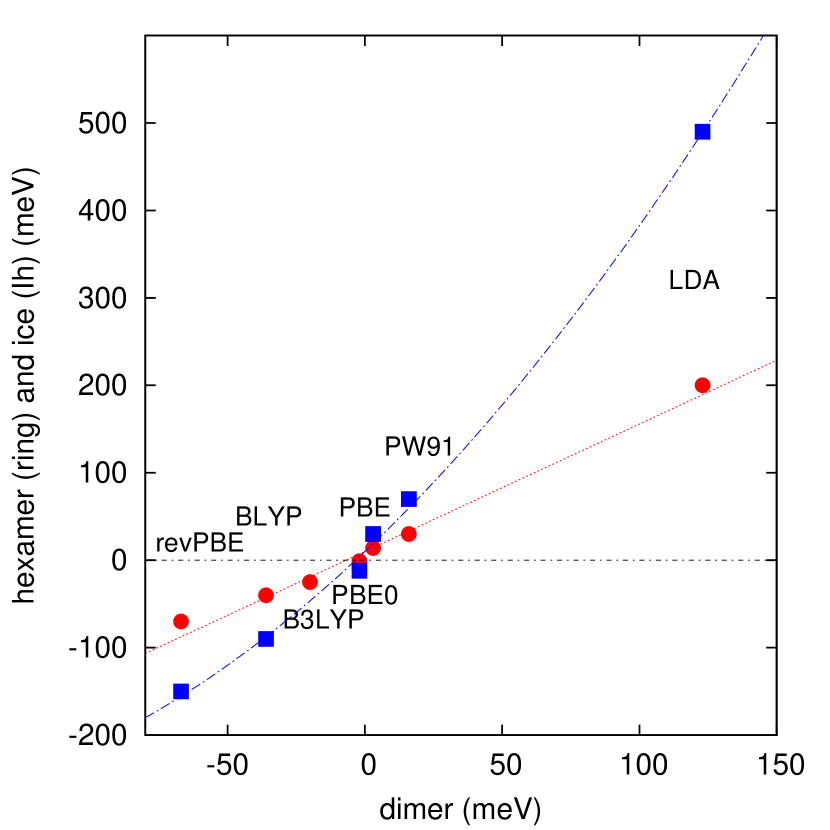
Figure 6: Errors of sublimation energy per monomer of ice Ih crystal (blue squares) and binding energy per monomer of ring-hexamer (red circles) plotted against error of dimer binding energy for chosen semi-local and hybrid exchange-correlation functionals.

The ordering of sublimation energies of ice Ih given by the GGAs in Table 4 is reminiscent of the ordering of GGA dimer energies (Table 1) and ring-hexamer energies (Table 3). To bring out the close relationship between these different manifestations of H-bond energy in water, we show in Fig. 6 plots of the GGA errors of the ice Ih sublimation energy and the ring-hexamer binding energy vs the corresponding error in the binding energy of the dimer in its global-minimum geometry. The close relationship between the three kinds of error is immediately apparent, and the smoothness of the curves indicates that for GGAs a knowledge of the error in the dimer energy suffices to predict the errors in the hexamer and ice Ih energies. It is noteworthy that the plots in Fig. 6 pass almost exactly through zero, something that would presumably not happen if GGA errors of polarizability caused a serious mis-description of the cooperative enhancement of H-bonding (see also Sec. IV). Hybrid approximations give more accurate polarizabilities than GGAs (Sec. II), so it is interesting to compare hybrids with their parent GGAs for the sublimation energy of ice Ih. Published information on this is very sparse, but we include in Fig. 6 the sublimation energy from PBE0, which is smaller than from PBE by ca. $40$ meV. This difference is certainly not negligible but only a part of this appears to be due to errors of cooperative enhancement.

We turn now to the energetics of compressed ice structures. Experiment tells us that as the pressure increases from atmospheric to $\sim 3$ GPa, the most stable low-temperature structures of ice pass through the series known for historical reasons as Ih, IX, II, XIII, XIV, XV, VIII. Fortunately, only a few key features of these structures need concern us here. The first is that the H₂O monomers retain their integrity in all the structures, though there are small changes in the intramolecular geometries. A second feature is that the number of H-bonds per monomer does not change, each monomer donating two H-bonds and accepting two from four of its neighbors. Even the O-O distance in each H-bond changes only a little through the series, the surprising fact being that it is slightly longer in the more compressed structures. Nonetheless, the volume per monomer decreases strongly from Ih to VIII, the volume in ice VIII being about two thirds that of ice Ih at zero pressure whalley1984a . This dramatic compression is entirely due to the ever closer approach of monomers that are not H-bonded to each other as we progress through the series. The coordination number is four in ice Ih but is eight in ice VIII, the O-O nearest-neighbor distance for the four non-H-bonded neighbors in ice VIII being slightly shorter than for the four H-bonded neighbors. Remarkably, in spite of the enormous compression, extrapolation of experimental data shows that the energies per monomer in the Ih and VIII structures, when both are at zero pressure, differ by a mere $33$ meV. This very small experimental energy difference is corroborated by both DMC and CCSD(T) calculations, which concur in predicting an energy difference between Ih and VIII of ca. $30$ meV/H₂O santra2011a ; gillan2013a .

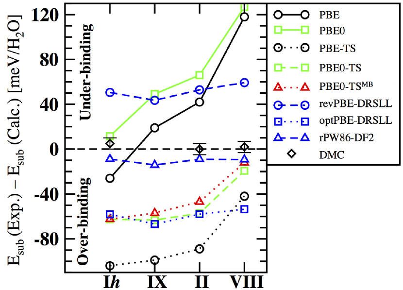
Figure 7: Differences $E_{\rm sub}({\rm Exp})-E_{\rm sub}({\rm Calc})$ between experimental and calculated values of the zero-pressure sublimation energies of the ice Ih, IX, II and VIII structures. Calculated values employ the semi-local functionals PBE and PBE0, a selection of dispersion-inclusive functionals, and diffusion Monte Carlo (DMC). Zero-point vibrational contributions to the experimental values have been subtracted. Adapted with permission from J. Chem. Phys. 139, 154702 (2013).

Semi-local XC functionals completely fail to reproduce the small energy differences between compressed ice structures and ice Ih, as can be seen from the calculated sublimation energies of ice VIII at zero pressure summarized in Table 4. With PBE and BLYP, the energy differences per monomer between zero-pressure ice VIII and Ih are calculated to be $177$ and $208$ meV respectively, which are $\sim 6$ times the experimental value of $33$ meV. We show in Fig. 7 plots of the errors of selected functionals for the sublimation energies of the sequence of increasingly compressed ice structures Ih, IX, II and VIII, reproduced from Ref. santra2013a . The rapidly growing errors of PBE along the sequence are striking, and we note that the hybrid functional PBE0 shows a very similar trend. Since PBE0 gives much better polarizabilities than PBE, the large semi-local errors clearly cannot stem mainly from errors of polarizability. The energies of compressed ice structures relative to ice Ih have been computed with a very wide range of semi-local functionals in Refs. kambara2012a ; brandenburg2015a . The functionals studied include the GGAs PW91, PBE, PBEsol, BLYP, RPBE and revPBE, the hybrid functionals PBE0 and B3LYP, the range-separated hybrid HSE06 and the meta-GGAs TPSS and M06L. In almost every case, the energy difference betwen ice Ih and VIII was found to be grossly overestimated. This indicates that essentially all semi-local and hybrid functionals suffer from the same kind of problem.

Why do semi-local and hybrid approximations incorrectly destabilize the compact, high-pressure ice structures relative to the more extended low-pressure structures? There appears to be a connection here with their behavior for the compact and extended configurations of the hexamer (Sec. V) and the larger water clusters (Sec. VI). For the hexamer, we saw the clear evidence that lack of dispersion is one of the main reasons for the wrong compact-extended balance given by semi-local approximations, and we will see the same for the ice structures. However, before reviewing dispersion-inclusive approximations for ice, we recall the many-body evidence that dispersion is not the only cause of trouble for the compact-extended balance in the hexamer. A similar many-body analysis has been reported for the errors of BLYP and PBE for the relative energies of high- and low-pressure ice structures gillan2013a . The outcome was that for BLYP the enormous overestimate of the energy difference between VIII and Ih is mainly a 2-body error, and that good relative energies are obtained once this error is corrected. However, the same is not true of PBE, where there appears to be a large beyond-2-body contribution to the error in relative energies.

A variety of dispersion-inclusive DFT approaches have been used to study the energetics of ambient and compressed ice phases, including Grimme DFT-D methods kambara2012a ; fang2013a ; brandenburg2015a , TS dispersion paired with PBE and PBE0 santra2011a ; santra2013a , and DRSLL-type approximations hamada2010a ; kolb2011a ; murray2012a ; fang2013a ; santra2013a . Most of these have paid particular attention to the energy differences between compressed structures and ice Ih, and in some cases have studied the equilibrium volumes of the structures and the transition pressures between them. All the different ways of including dispersion give a large improvement in the relative energies of the extended and compact structures. However, not all the methods are equally good, because in some cases the improvement in the relative energies is accompanied by a worsening of the sublimation energy of the ice Ih structure.

The range of results that can be given by different dispersion-inclusive methods is illustrated by the work of Ref. santra2013a , where the performance of different versions of the TS and DRSLL-type schemes was compared (see Fig. 7). The work showed that the original version of DRSLL based on revPBE dion2004a , referred to here as revPBE-DRSLL, gives very satisfactory energies of the structures IX, II and VIII relative to ice Ih, but that all the structures are underbound compared with experiment by $\sim 50$ meV. This is expected, because the excessive exchange-repulsion of revPBE-DRSLL generally gives underbinding in H-bonded systems, as we saw for the water dimer and ring-hexamer in Secs. III and V. The optPBE-DRSLL approximation has weaker exchange-repulsion, and performs better for H-bonding energies, giving much better dimer and ring-hexamer energies. It also gives accurate energies of the IX, II and VIII structures relative to Ih, but all these structures are now overbound. However, the revised version of DRSLL due to Lee et al. lee2010a , which we refer to as rPW86-DF2, performs very well for both the relative energies and the sublimation energies of the the ice structures, (Fig. 7), as was also found by Murray and Galli murray2012a . Not reported in Fig. 7 but given in Table 4 are results for optB88-DRSLL. As with optPBE-DRSLL, it describes the energy difference between ice I and VIII well but overbinds both phases.

Predictions from the scheme of Tkatchenko and Scheffler tkatchenko2009a in which dispersion is added to PBE or PBE0 provide an instructive contrast. Since ice Ih is already somewhat overbound with PBE, it is no surprise that PBE-TS overbinds this structure by over $100$ meV/monomer. Nevertheless, PBE-TS gives a considerable improvement over PBE itself for the relative energies, though it is not as good as any of the DRSLL-type methods. The PBE0-TS approximation also overbinds ice Ih, but only by $\sim 60$ meV, and the difference between the energies of the VIII and Ih structures is also slightly better than with PBE-TS. Also included in Fig. 7 are the predictions obtained by adding many-body dispersion tkatchenko2012a to PBE0. These differ only slightly from PBE0-TS, so that the effects of beyond-2-body dispersion appear to be very small for these ice structures, as might be expected from previous work on the contribution of 3-body dispersion to the energetics of ice vonlilienfeld2010a .

Insight into the performance of the DFT-D methods of Grimme et al. for the energetics of ice structures can be gained from Refs. brandenburg2015a ; kambara2012a , both of which demonstrate the major improvements brought by the inclusion of dispersion. In the first of these papers, the binding energies of $10$ ice structures were computed with Grimme D3 dispersion added to a variety of semi-local functionals. These DFT-D3 approximations give reasonably good binding energies of ice Ih, except for PBE-D3, which is overbound by an unacceptable $\sim 140$ meV. The PBE-D3 approximation also gives a greatly overestimated value of $\sim 130$ meV for the energy difference between the ice VIII and Ih structures, which is also overestimated by the other DFT-D3 approximations, though less seriously.

Turning now to the equilibrium volumes, we report in Table 5 results for ice I and VIII from a selection of GGAs, PBE0, and several dispersion inclusive functionals. By and large, the trends found for sublimation energies are mirrored in the predictions of equilibrium volumes. For example, at the GGA level the sublimation energies decrease from PBE to BLYP to revPBE, while the equilibrium volumes show the opposite trend, with revPBE $>$ BLYP $>$ PBE. The errors in the volumes for ice Ih predicted by GGAs are less than $4$ %, but they are much larger for ice VIII, in the range $9$ - $28$ %, as might be expected from the substantial under-binding of ice VIII predicted by GGAs. It has been shown that in ice VIII zero-point effects increase the equilibrium volume by ca. $5$ % murray2012a ; santra2013a ; brandenburg2015a , so in assessing the errors in the predicted volumes we compare with the experimental volume reduced by this amount. Zero-point corrections to the equilibrium volume are much smaller for ice Ih murray2012a ; santra2013a ; brandenburg2015a , so for this phase we simply compare with the uncorrected experimental value. As shown in Table 5, accounting for exact exchange by going from PBE to PBE0 does little to reduce the errors in the volumes. By contrast, dispersion has a significant impact on the volumes, generally decreasing them, as one would expect. However, the results are very sensitive to the particular choice of dispersion inclusive functional. Of the functionals reported, BLYP-D3, revPBE-D3, optPBE-DRSLL do reasonably well for the two phases, while revPBE-DRSLL stands out as offering the worst performance (volume of ice VIII overestimated by 20%). Despite performing very well in terms of sublimation energies, the volumes predicted by rPW86-DF2 are rather disappointing. Overall, it is clear that for predictions of equilibrium volumes in the ice phases there is still considerable room for improvement.

We noted at the start of this Section that proton-disordered ice phases such as Ih transform to proton-ordered structures at low temperatures. This is a subtle phenomenon in both experiment and theory. The very slow kinetics of molecular reorientation at low temperatures makes it difficult to measure the true thermodynamic transition temperatures accurately, and unambiguous identification of the symmetry of the proton-ordered phase has sometimes been controversial. Widely used force fields sometimes yield completely erroneous predictions for these transitions buch1998a , so that there has been considerable interest in DFT treatments kuo2004c ; singer2005a ; knight2006a ; tribello2006a ; tribello2006b ; fan2010a ; pan2010a ; singer2011a ; delben2014a .

The transformation of ice Ih to a low-temperature ordered phase was conjectured over 60 years ago bjerrum1952a , but the experimental evidence for a transition near $72$ K appeared only more recently kawada1972a ; tajima1982a . Simple electrostatic arguments bjerrum1952a ; davidson1984a ; buch1998a suggest that the low-temperature phase ice XI should be antiferroelectric, but this expectation is contradicted by diffraction and thermal depolarization experiments jackson1995a ; jackson1997a , which indicate that it is actually ferroelectric, though the interpretation of the experiments has been challenged iedema1998a . DFT calculations based on the BLYP functional singer2005a , in conjunction with graph-theoretic methods used to enumerate H-bonding topologies kuo2001a ; kuo2003a , support the ferroelectric assignment. The parameterized models produced in the course of this computational approach, when used in statistical-mechanical calculations, yield a transition temperature of $98$ K singer2005a in respectable agreement with the experimental value. It was shown later knight2006a ; tribello2006b ; fan2010a that this outcome is not significantly altered if other XC functionals are used in place of BLYP. Remarkably, even the unsophisticated LDA functional yields essentially the same result tribello2006b . It has been argued from this that the electrostatic part of the energy dominates the energetics of proton ordering, as originally proposed by Bjerrum bjerrum1952a , and that the inability of common force fields to describe the energetics correctly arises from their failure to reproduce the high multipole moments of the charge distribution of the H₂O monomer tribello2006b ; fan2010a . Another approach to the transformation between ice Ih and XI was taken by Ref. schoenherr2014a . There, MC sampling based on the dispersion-inclusive functionals PBE-D2 and BLYP-D2, and also their hybrid counterparts PBE0-D2 and B3LYP-D2 was used to compute the static dielectric constant $\epsilon$ and the ice Ih/XI transition temperature. It was found that PBE0-D2 at $T=273$ K gives $\epsilon$ roughly $20$ % greater than the experimental value of $95$, while the value with PBE-D2 is roughly $50$ % greater, so that the over-polarizability of the H₂O molecule with PBE (see Sec. II) is clearly significant. The transition temperature computed with PBE0-D2 in this work was in the range $70-80$ K, in satisfactory agreement with experiment.

Calculations combining DFT with graph-theoretic methods have also been successful in treating the transformation of other proton-disordered phases to their low-temperature ordered counterparts, including ice VII to VIII knight2006a ; tribello2006b , XII to XIV tribello2006a and V to XIII knight2008a . Where comparison with experiment is possible, the symmetries of the ordered phases are correctly predicted, and the transition temperatures are approximately correct. However, there appears to be one exception, namely the transition from ice VI to XV, where experiment shows the ordered phase to be antiferroelectric salzmann2009a , while DFT calculations consistently make the most stable structure ferroelectric knight2005a ; delben2014a . Hybrid and dispersion-inclusive functionals give the same result, as do calculations based on MP2 and the random phase approximation (RPA) delben2014a , which are expected to be even more accurate. In discussion of the possible origins of this paradox, it was suggested in Ref. delben2014a that the so-called “tin-foil” boundary conditions implicitly used in conventional electronic-structure calculations on periodic systems may not be appropriate for the ice VI-XV transition. It was shown that if instead the boundary conditions are allowed to reflect the electrostatic environment in which ice XV grows, then the ferroelectric phase may be sufficiently disfavored for the antiferroelectric phase to become more stable. The experimental work of Ref. shephard2015a appears to offer support for this idea.

Although hexagonal ice Ih is the naturally occurring form under ambient conditions, there is evidence that the cubic variant known as ice Ic can form in the upper atmosphere zhang2006a ; murray2006a , though it is not yet clear whether pure ice Ic or only a disordered mixture of ice Ic and Ih is formed malkin2012a ; kuhs2012a . In either case, the question of the energy difference between the two forms of ice is of some importance for environmental science. Raza et al. raza2011a tackled this question by performing DFT calculations on the lowest-energy proton-ordered forms of the two crystal structures, using the XC functionals PBE, PBE0, BLYP-D3 and optPBE-DRSLL; accurate reference calculations with DMC were also reported. The conclusion from their work was that the two structures are isoenergetic within the technical tolerances of the calculations, the indication being that the energy difference is less than $1$ meV/monomer. This conclusion is supported by later work from Geiger et al. geiger2014a . It has been shown very recently engel2015a that the clear preference for ice Ih over ice Ic observed in nature may be due to the difference of anharmonic vibrational energy between the two phases.

We conclude this Section by commenting briefly on the influence of isotope effects on the properties of ice. In almost solids, the replacement of a heavier isotope by a lighter one causes an expansion of the equilibrium volume. The reason is that expansion normally reduces the vibrational frequencies and hence the zero-point energy, the reduction being greater for lighter isotopes. It therefore comes as a surprise that the equilibrium volume of the H₂O form of ice Ih is less than the D₂O form roettger1994a . It was shown recently pamuk2012a that this anomalous isotope effect occurs because expansion of ice weakens the H-bonds, which in turn strengthens the intramolecular O-H bonds, thus increasing their frequency. However, the consequences of this increase are partially canceled by the softening of other vibrational modes. Some of the common force-fields for water wrongly predict a normal isotope effect, but DFT calculations generally give the observed anomalous isotope effect, at least with the XC functionals examined so far. It has been noted recently pamuk2015a that the same mechanism leads to an interesting isotope effect on the temperature of the transition from ice Ih to XI.

VIII DFT simulation of liquid water

Our review of DFT work on liquid water will be concerned with the structure of the liquid, its thermodynamic properties, and the dynamics of the molecules. We shall pay particular attention to the three radial distribution functions (rdfs) $g_{\alpha\beta}(r)$, the density $\rho_{\rm eq}$ of the liquid at near-ambient pressure, and the self-diffusion coefficient $D$, all of which are available from experiment. Some aspects of the DFT simulation of the liquid have recently been reviewed by Khaliullin and Kühne khaliullin2013a .

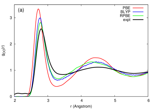
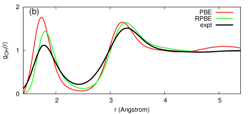
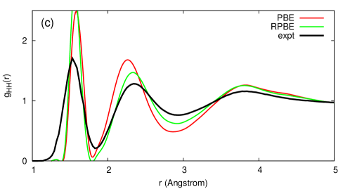
Figure 8: Panels (a), (b) and (c) show O-O, O-H and H-H radial distribution functions (rdfs) of liquid water at ambient temperature and experimental density from experiment and from MD simulations based on the PBE and RPBE approximations (results from BLYP are also shown for $g_{\rm OO}(r)$). Simulation rdfs with PBE and RPBE are from Ref. forster-tonigold2014a and results with BLYP from Ref. bankura2014a . Experimental rdf $g_{\rm OO}(r)$ is from high-energy x-ray diffraction measurements skinner2013a , and rdfs $g_{\rm OH}(r)$ and $g_{\rm HH}(r)$ are from joint refinement of neutron and x-ray diffraction measurements soper2007a .

As initial orientation, we refer to panel (a) of Fig. 8, showing the O-O rdf $g_{\rm OO}(r)$ from recent high-energy x-ray diffraction measurements skinner2013a performed at temperatures close to $297$ K. (The simulation results shown in the Figure will be discussed later.) It is worth commenting here that there have been many experimental measurements of $g_{\rm OO}(r)$ over the years (see literature cited in Ref. skinner2013a ), and there has been considerable controversy about the height of the first peak, but the measurements we compare with here are generally accepted to supersede earlier work. The first peak at O-O separation $R_{\rm OO}=2.80$ Å and the second peak at $R_{\rm OO}=4.5$ Å correspond rather closely to the first- and second-neighbor O-O distances in ice Ih. The first-neighbor coordination number $N_{1}$ in the liquid is not uniquely defined, but is conventionally taken to be the integral $N_{1}=4\pi n\int_{0}^{r_{\rm min}}dr\;r^{2}g_{\rm OO}(r)$ under the first peak ($n$ is the bulk number density) up to the radius $r_{\rm OO}^{\rm min}$ of the first minimum. The diffraction experiments all give a coordination number $N_{1}$ in the region of $4.3$, which is consistent with roughly fourfold tetrahedral bonding. However, there is clearly considerable disorder, since the experimental $g_{\rm OO}(r)$ is quite close to unity over the range $3.0<R_{\rm OO}<4.0$ Å, throughout which there are no neighbors in ice Ih; all diffraction measurements agree that the value of $g_{\rm OO}(r)$ at its first minimum is $g_{\rm OO}^{\rm min}=0.84\pm 0.02$. This means that there is substantial penetration of molecules from the second shell into the shell of H-bonded first neighbors.

The phenomenon of cross-shell penetration is crucially important in liquid water, and is closely linked to the density increase on melting. The amount of penetration is sensitive to pressure, and diffraction experiments straessle2006a ; weck2009a ; katayama2010a show that a pressure of only $\sim 1$ GPa ($10$ kbar) is enough to increase the O-O coordination number from ca. $4$ to ca. $8$, an effect that occurs by collapse of the second shell into the region of the first shell, without significant breaking of H-bonds straessle2006a . This implies that the penetration in the liquid is closely related to changes of ice structure with increase of pressure, exemplified by the presence of non-H-bonded first neighbors at approximately the same distance as the H-bonded neighbors in ice VIII. Cross-shell penetration also appears to be intimately linked to diffusion, which requires molecules to cross the region $3.0<R_{\rm OO}<4.0$ Å; since the lifetime of H-bonds under ambient conditions is estimated to be in the region of $1$ ps luzar1996a ; bankura2014a , this crossing must be frequent.

We saw in Sec. VII that GGAs grossly exaggerate the energy difference betwen the extended ice Ih structure and compact structures such as ice VIII. They make it too difficult for a molecule to approach another molecule that is already H-bonded to four others, and the problem is cured by accounting for dispersion. We can anticipate that the same mechanisms will operate in the liquid, so that GGAs will generally hinder penetration, making the liquid over-structured and under-diffusive, with a high pressure needed to maintain the experimental density. Accordingly, a leading theme of our survey of DFT work on the liquid will be the concerted efforts of the past few years to address the difficulties of liquid structure, thermodynamics and dynamics with dispersion-inclusive methods. We shall see that these efforts have enjoyed considerable success, but it will also become apparent that current dispersion-inclusive methods are still immature, and that over-correction can be as much of a peril as under-correction. We shall also see that purely technical issues have sometimes made it difficult to judge the true capabilities of any given DFT method.

VIII.1 Technical issues

It is not trivial to assess how well an XC functional performs for the liquid, because the first-principles simulation of the liquid raises many tricky technical issues that are completely absent from the study of clusters or static ice structures. Thermodynamic, structural and dynamical quantities such as the pressure $P$, the radial distribution functions $g_{\alpha\beta}(r)$ and the self-diffusion coefficient $D$ are all calculated as time averages over the duration of the simulation, which must be long enough to yield useful statistical accuracy. Furthermore, collection of the data to be averaged can only begin after the system has been ‘equilibrated’, i.e. simulated for long enough to ensure that memory of the initial conditions has been lost. The problems of equilibration and time averaging are exacerbated in water by the wide separation of timescales between intramolecular and intermolecular motions, which hinders energy transfer between these degrees of freedom. Memory times can be reduced by the use of thermostats, but dynamical quantities may then be falsified. In MD simulations of water based on force fields, the equilibration and production phases commonly have durations of $100$ ps or more (see e.g. Refs. fernandez2006a ; fanourgakis2008a ; habershon2009a ), but such durations have been impractical in DFT simulations until recently kuehne2009a ; khaliullin2013a . (In the earliest first-principles simulations of water laasonen1993a ; tuckerman1994a ; sprik1996a ; silvestrelli1999a ; silvestrelli1999b , these durations were between $2$ and $10$ ps.)

First-principles simulations can be performed by Born-Oppenheimer MD (BOMD), in which the Kohn-Sham orbitals are relaxed to the self-consistent ground state at every time step, or by Car-Parrinello MD (CPMD), in which the orbitals are treated as dynamical degrees of freedom, their dynamics being governed by a fictitious mass $\mu$. The method known as second-generation CPMD kuehne2007a ; kuehne2009a ; kuehne2013a combines the strengths of these two techniques. In addition, first-principles Monte Carlo simulation is also feasible kuo2004b . If rigorously implemented, all these techniques should be equivalent, but practical compromises in the setting of technical parameters can cause differences. It took several years to discover that the close agreement with experiment reported in some early papers silvestrelli1999a ; silvestrelli1999b ; izvekov2002a was partly due to simulation errors caused by $\mu$ being set too high asthagiri2003a ; grossman2004a ; schwegler2004a ; kuo2004b ; fernandez-serra2004a ; vandevondele2005a ; sit2005a . Significant discrepancies may also arise from the use of different statistical-mechanical ensembles, which are expected to yield identical results in the thermodynamic limit, but not in finite systems. Inadequate basis sets too can be a source of inaccuracy. System-size errors present yet another hazard: ideally, the size of the periodically repeated simulation cell should be systematically increased at constant density until the observables of interest settle to converged values, but in practice the cell size is constrained by the computer budget.

These and other technical difficulties plagued much of the pioneering DFT work on water, but the problems started to be clearly identified and addressed around 10 years ago asthagiri2003a ; grossman2004a ; schwegler2004a ; fernandez-serra2004a ; kuo2004b ; sit2005a and it is now understood in principle how to bring most of them under firm control. The conditions necessary for adequate equilibration, statistical averaging and thermostating were analyzed in Ref. vandevondele2005a . The equivalence of Car-Parrinello and Born-Oppenheimer dynamics and the range of fictitious mass needed to ensure this equivalence were established in Refs. schwegler2004a ; kuo2006a . System-size errors have turned out to be only a minor concern for many thermodynamic and structural quantities, provided systems of 64 molecules or more are used vandevondele2005a ; kuehne2009a , although substantial (but well understood) size corrections are needed for the diffusivity kuehne2009a . Increasing computer power has made it much less necessary to compromise on basis-set completeness. Nevertheless, technical uncertainties continue to be troublesome even now, as will become clear below.

VIII.2 Quantum nuclear effects

In addition to the technical issues just outlined, there is also the physical phenomenon of quantum nuclear effects (QNE). Almost all first-principles simulations of water have treated the nuclei classically, but it is well known from diffraction experiments soper2008a and force-field simulations fanourgakis2008a ; habershon2009a that QNE due to the light mass of hydrogen are not negligible. Path-integral simulation chen2003a ; morrone2008a ; ceriotti2013a ; wang2014a allows QNE to be included almost exactly, at least for thermodyamics and structure, but the computational cost then escalates still further. (We note, however, that recent algorithmic developments ceriotti2014a mitigate the additional cost.) If QNE are not included in simulations of the liquid, then perfect agreement with experimental data cannot be expected, but it is not straightforward to separate errors due to neglect of QNE from those due to inaccuracy of the XC functional. We will note the possible influence of QNE where appropriate in the following, but we do not aim to treat this important matter in depth in this review, since QNE in water have recently been reviewed by Ceriotti et al. ceriotti2015a .

VIII.3 GGAs and hybrids

We start our survey of DFT methods for liquid water by focusing on GGAs, and since BLYP and PBE have been the most widely used GGAs we discuss these first. After this, we summarize the rather few simulations that have been performed with other GGAs and with hybrid functionals. Most simulations have been performed at constant volume, corresponding to an experimental density close to $1$ g/cm³, and these conditions apply unless we mention otherwise. A summary of the main features of the simulations reviewed here is provided in Tables 6 and 7.

Well over $20$ substantial simulations of the near-ambient liquid have been reported with the BLYP functional since the resolution of the technical difficulties mentioned above (references in Table 6). Most of these simulations appear to be free of major technical limitations, and there is now a reasonable consensus about the properties predicted by BLYP. Comparison of the O-O rdf $g_{\rm OO}(r)$ with neutron and x-ray diffraction data is generally regarded as the cleanest way of testing the liquid structure, since this rdf is much less affected by QNE than $g_{\rm OH}(r)$ and $g_{\rm HH}(r)$ fanourgakis2008a ; habershon2009a . An example of the comparison between BLYP and experiment is shown in panel (a) of Fig. 8. As in most BLYP-based simulations published over the past $10$ years, the liquid is somewhat over-structured, the height of the first peak and the depth of the first minimum being somewhat exaggerated, but the radial positions of all the main features agree well with experiment (see Table 6). Many of the BLYP-based simulations have reported values of the self-diffusion coefficient $D$, for which accurate experimental values are available over a range of temperatures for both light and heavy water. As might be expected from the over-structuring, the values of $D$ given by BLYP (see Table 6) are lower than the experimental values, usually by a factor of $\sim 3$.

Some BLYP-based studies have also reported the O-H and H-H rdfs $g_{\rm OH}(r)$ and $g_{\rm HH}(r)$. The O-H rdf is instructive, because its peak at $r\simeq 1.75$ Å directly probes the H-bond between the donor H and the acceptor O. All the BLYP-based simulations that reported $g_{\rm OH}(r)$ (see e.g. Refs. grossman2004a ; lee2006a ; morrone2008a ; bartok2013a ; bankura2014a ) found the height of this H-bond peak to be overestimated by $\sim 30$ %. Both force-field and DFT-based simulations that have accounted for QNE by the path-integral technique fanourgakis2008a ; morrone2008a suggest that the quantum nature of the proton might explain as much as half of this overstructuring. However, there is little doubt that the other half is due to errors of the BLYP functional. The overstructuring also affects $g_{\rm HH}(r)$ grossman2004a ; lee2006a ; morrone2008a ; bartok2013a .

The disagreements with experiment are more severe with the PBE functional. All the PBE-based simulations reported over the past 10 years (references in Table 7) give a substantially over-structured liquid, the height of the first peak and the first minimum in $g_{\rm OO}(r)$ being typically $g_{\rm OO}^{\rm max}\simeq 3.4$ and $g_{\rm OO}^{\rm min}\simeq 0.4$ respectively, compared with the experimental values of $2.57$ and $0.84$ (Fig. 8 and Table 7). The very deep first minimum is particularly significant, since it indicates a strong suppression of close approaches by non-H-bonded monomers. The overstructuring is even more striking in $g_{\rm OH}(r)$ and $g_{\rm HH}(r)$ schwegler2004a ; forster-tonigold2014a , with the height of the H-bond peak in $g_{\rm OH}(r)$ at $r\simeq 1.75$ Å being overestimated by $\sim 50$ % and similarly large errors in $g_{\rm HH}(r)$ (see Fig. 8). Correspondingly, the self-diffusion coefficient is grossly underestimated, being too low compared with experiment by about a factor of $10$. The only other GGAs that have seen more than occasional use in water simulations are revPBE and the closely related RPBE (references in Table 7). Almost all the simulations reported with these functionals agree that they yield a liquid with much less structure (see Fig. 8) and a higher diffusivity than BLYP and PBE (but see Ref. kuehne2009a ).

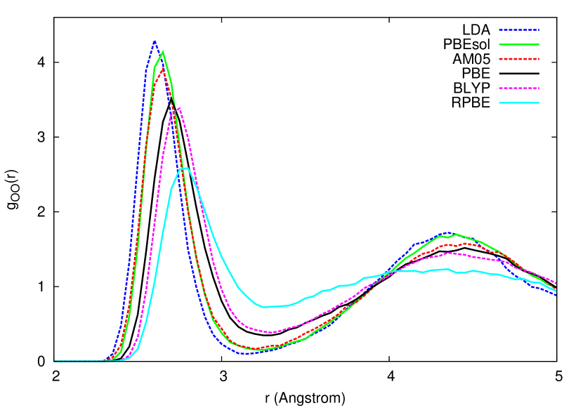
Figure 9: The O-O rdf of liquid water at experimental density and $T=300$ K computed with a series of semi-local functionals. Adapted from Ref. mattsson2009a , with permission.

The foregoing comparisons show that the structure and diffusivity of the liquid differ substantially for different GGAs. It would be surprising if this were not so, since we saw in Secs. III, V and VII that the H-bond energy depends strongly on the choice of GGA, and Fig. 6 demonstrates the close relationship between the errors in GGA binding energies of clusters and ice. The properties of the liquid at specified density and temperature presumably depend on the H-bond energy, and it is natural to ask if the trends in predicted structure and diffusivity correspond in some way to the trends illustrated in Fig. 6. The paper of Mattsson and Mattsson mattsson2009a appears to be the only one that has systematically addressed this important question, and we reproduce in Fig. 9 their O-O rdfs computed at $T=300$ K with the series of semi-local functionals RPBE, BLYP, PBE, AM05, PBEsol, LDA. The functionals that yield highly overstructured water are likely to give a glassy state at $300$ K, but the trend of increasing structural ordering along this series is nonetheless clear, as is the steady leftward shift of the first-peak position $r_{\rm OO}^{\rm max}$. The order of this trend is also the order of increasing dimer binding energy (see Table 1), with the possible exception of the AM05 approximation, which appears to give a slightly lower dimer binding energy than PBE mattsson2009a . We return later to the close correlation between structural ordering in the liquid and H-bond energy.

As noted in Secs. II and IV, GGAs generally overestimate the polarizability of the water molecule by $\sim 10$ %, so that they might be expected to exaggerate the cooperative enhancement of H-bonding in condensed phases. Furthermore, they underestimate the stretching frequencies of the water monomer by $3-5$ %, and the excessive flexibility of the intramolecular OH bonds may further strengthen H-bonding. These are reasons for expecting hybrids to soften the structure of the liquid, since they give better polarizabilities and monomer frequencies. The evidence on this point is not entirely unanimous. The early simulations of Todorova et al. todorova2006a , performed at $T=350$ K, showed a substantial softening when the PBE functional is replaced by PBE0, with $g_{\rm OO}^{\rm max}$ decreasing from $2.99$ to $2.58$ and $g_{\rm OO}^{\rm min}$ increasing from $0.47$ to $0.73$. Subsequent work of Zhang et al. zhang2011a ; zhang2011b and DiStasio et al. distasio2014a also found that PBE0 produces a softer structure than PBE, but the softening found in the latter work is fairly weak, with $g_{\rm OO}^{\rm max}$ decreasing from $3.22$ to $2.98$ and $g_{\rm OO}^{\rm min}$ increasing from $0.38$ to $0.52$. Simulations reported by Guidon et al. guidon2008a ; guidon2010a found very little change in structure from PBE to PBE0 even when the fraction of exact exchange in PBE0 is increased from its normal value of $25$ % all the way to $100$ %. However, there is very recent evidence delben2015a that basis-set errors in the ADM (Auxiliary Density Matrix) technique employed in Ref. guidon2010a may have had the effect of slightly hardening the structure, so that the small softening due to exact exchange was perhaps masked.

All the comparisons we have presented so far for GGA and hybrid functionals have been for fixed densities very close to the experimental value. However, a major failing of GGAs is that they give very inaccurate pressure-volume relations for the liquid. One manifestation of this is that if simulations are performed at zero pressure, for example by working with the ($NPT$) ensemble, then the average density $\rho_{\rm eq}$ deviates markedly from the experimental value. Equivalently, in simulations at fixed volume, the average pressure is poorly predicted. Since pressure is routinely calculated (though not always reported) in constant-volume simulations, these errors are straightforward to detect.

The simulations of Kuo et al. kuo2004a , in which BLYP-based simulations were used to study the density profile in a water slab with free surfaces, suggested that BLYP underestimates $\rho_{\rm eq}$ by $\sim 15$ %, giving a value of $\sim 0.85$ g/cm³. An underestimate of this order was confirmed soon afterwards by simulations performed in the ($N,P,T$) ensemble using MC sampling mcgrath2005a , which also employed the BLYP functional. These indicated an equilibrium density at $T=298$ K of ca. $0.80$ g/cm³. This substantial underestimate has since been confirmed by many studies schmidt2009a ; baer2011a ; ma2012a ; lin2012a ; bartok2013a ; alfe2013a ; delben2013a , though the numerical values have been surprisingly variable, with $\rho_{\rm eq}$ ranging from $0.74$ g/cm³ schmidt2009a to $0.92$ g/cm³ lin2012a ; ma2012a . Related work has shown that revPBE gives even lower densities wang2011a ; lin2012a , with $\rho_{\rm eq}$ ranging from $0.69$ to $0.85$ g/cm³. PBE also underestimates the density schmidt2009a ; wang2011a ; lin2012a ; corsetti2013a ; miceli2015a ; gaiduk2015a , but more modestly, with $\rho_{\rm eq}$ varying from $0.86$ to $0.96$ g/cm³ in different studies. One of the few DFT studies of the moderately compressed liquid is that of Ref. alfe2014a , which reported BLYP and PBE simulations at a density of $1.245$ g/cm³, and $T=420$ K, where the experimental pressure is $15$ kbar. As would be expected from the predictions of these GGAs near ambient conditions, BLYP was found to give a greatly overestimated pressure of $32$ kbar, while the PBE value of $24$ kbar was less in error. Values of the equilibrium density from GGA simulations are summarized in Tables 6 and 7, and we note that all studies that compare values of $\rho_{\rm eq}$ predicted by different functionals agree that the estimated densities come in the order revPBE $<$ BLYP $<$ PBE $<$ expt. This trend is consistent with the natural supposition that $\rho_{\rm eq}$ computed with GGAs will tend to increase with increasing H-bond energy.

The large body of work based on semi-local and hybrid functionals thus indicates that increasing the H-bond energy enhances the ordering of the liquid and reduces the diffusivity, and also (slightly more tentatively) increases the equilibrium density. However, functionals that give a more realistic degree of ordering and diffusivity also severely underestimate the equilibrium density. This comes as no surprise, since the work on clusters and ice structures taught us that to get both good H-bond energies and a correct extended-compact balance, dispersion is needed.

VIII.4 Dispersion-inclusive approximations

With these ideas in mind, we now turn to simulations of the liquid performed with dispersion-inclusive DFT approximations, which have been reported using various representations of dispersion added to a number of different GGAs and hybrids. The main features of the simulations reviewed here are summarized in Tables 8 and 9. We start by discussing the very popular approach in which correction potentials are added to the BLYP functional schmidt2009a ; jonchiere2011a ; mcgrath2011a ; baer2011a ; yoo2011a ; ma2012a ; delben2013a ; lin2009a ; lin2012a ; bankura2014a . As noted in the Sections on clusters and ice structures and in the Appendix, there are a number of methods of this type, including the different versions of BLYP-D due to the Grimme group grimme2004a ; grimme2006a ; grimme2010a , and DCACP-corrected BLYP as developed by Rothlisberger and co-workers vonlilienfeld2004a . It is convenient to include here simulations based on BLYP+GAP bartok2013a ; alfe2013a , which corrects almost exactly for the 1- and 2-body errors of BLYP and therefore accounts for dispersion, which is expected to be mainly a 2-body interaction in water systems vonlilienfeld2010a . We already know that all these methods give a much better description of clusters and ice structures than BLYP itself, so there is good reason to hope for improvements in the liquid as well.

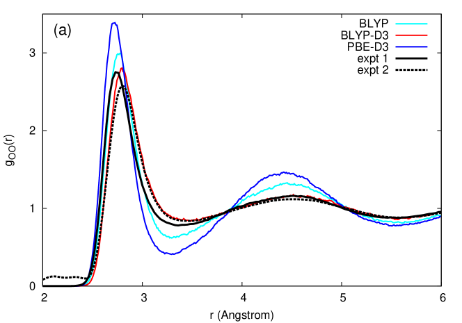
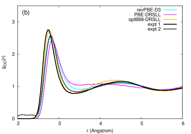
Figure 10: Oxygen-oxygen rdf $g_{\rm OO}(r)$ of liquid water from BLYP and dispersion-inclusive DFT approximations, compared with experiment. Simulation results are from Ref. bankura2014a . Experimental results are from joint refinement of neutron and x-ray measurements soper2007a (expt 1: solid black curve) and from high-energy x-ray diffraction measurements skinner2013a (expt 2: dashed black curve).

Almost all the simulations based on corrected BLYP agree that the addition of dispersion substantially increases the equilibrium density $\rho_{\rm eq}$, softens the liquid structure, and increases the diffusivity. Since uncorrected BLYP considerably underestimates $\rho_{\rm eq}$, somewhat overstructures the liquid, and suppresses diffusion, this means that the changes brought by dispersion are all in the right direction. The large differences in the liquid properties given by different simulations based on uncorrected BLYP (see above) carry over to dispersion-corrected BLYP, as can be seen in Table 8. Focusing on the areas of agreement first, we note from the Table that all the correction methods increase $\rho_{\rm eq}$ by between $0.10$ and $0.25$ g/cm³ schmidt2009a ; baer2011a ; lin2012a ; ma2012a ; delben2013a ; alfe2013a . Taken together, the calculations suggest that with dispersion-corrected BLYP $\rho_{\rm eq}$ is slightly overestimated, perhaps by $\sim 5$ %. This is not unexpected, since we saw that BLYP corrected for 1- and 2-body errors using GAP overbinds both water clusters and ice structures, and tends to compress both. The liquid structure is softened in similar ways by the different forms of dispersion-corrected BLYP, the value of $g_{\rm OO}^{\rm max}$ being lowered by $\sim 0.30$ and the value of $g_{\rm OO}^{\rm min}$ being raised by $\sim 0.20$. Perhaps most important is that most of the simulations give $g_{\rm OO}^{\rm min}\simeq 0.78$, which is close to the well established experimental value of $0.84$ and is very much better than the value of $g_{\rm OO}^{\rm min}\simeq 0.60$ given by uncorrected BLYP. An example of the softening effect of adding dispersion to BLYP is shown in Fig. 10. (We include in this Figure $g_{\rm OO}(r)$ obtained from the recent high-energy x-ray data of Ref. skinner2013a , which is expected to be more accurate than earlier experimental measurements of $g_{\rm OO}(r)$.) As expected from the structural softening, all the simulations agree that correcting BLYP for dispersion increases the diffusion coefficient $D$ by a factor of $2-3$, thus bringing it into fair agreement with experiment (correction for system-size errors is essential in making this comparison, as emphasized above). The general consensus is that BLYP corrected for dispersion, whether in the form of BLYP-D, BLYP-DCACP or BLYP+GAP is a considerable improvement over BLYP itself, as might be hoped from the reasonable performance of these approximations for clusters and ice structures.

Two caveats should be noted, however. First, the BLYP-D2 simulation of Ma et al. ma2012a , which gave a high $\rho_{\rm eq}$ of $1.07$ g/cm³, predicted a significant under-structuring of the liquid. The authors of Ref. ma2012a stress that their simulations are performed very close to the CBS limit, and they suggest that the basis sets used to generate Grimme’s D2 representation of dispersion may not have been large enough to guarantee compatibility with their own basis sets. This suggestion appears to deserve further investigation. Second, dispersion-corrected BLYP cannot be regarded as fully satisfactory, since we know that it suffers from beyond-2-body over-binding, which is presumably the reason why its value of $\rho_{\rm eq}$ is too high by a few percent in most of the simulations.

The PBE approximation has rivalled BLYP in popularity as a starting point for adding dispersion, with a wide variety of techniques used to represent the dispersion. Simulations of liquid water have been published using the representations of dispersion due to Grimme schmidt2009a ; delben2013a ; forster-tonigold2014a ; gaiduk2015a and Tkatchenko-Scheffler distasio2014a , as well as the DCACP method lin2012a . Furthermore, several simulations have been reported in which the non-local correlation functional pioneered by Lundqvist, Langreth and co-workers is paired with PBE wang2011a ; zhang2011a ; zhang2011b . We also refer here to a simulation of the compressed liquid based on GAP-corrected PBE alfe2014a . As expected, the addition of dispersion to PBE generally increases $\rho_{\rm eq}$, though this leads to an overestimate by $\sim 13$ % in the case of PBE-DRSLL (see Table 8). Interestingly, the almost exact GAP correction for 1- and 2-body errors gives very little change of pressure in the compressed liquid at density $1.245$ g/cm³ alfe2014a , so that the error in the pressure given by PBE appears to be mainly a beyond-2-body effect.

With PBE as the starting approximation, the effect of dispersion on the liquid structure depends strongly on the method used to represent dispersion. The simulations based on Grimme PBE-D schmidt2009a ; delben2013a ; forster-tonigold2014a ; bankura2014a ; gaiduk2015a all show that the addition of dispersion does not cure the marked over-structuring given by PBE itself. In these simulations, the values of $g_{\rm OO}^{\rm max}$ and $g_{\rm OO}^{\rm min}$ are $3.2$ - $3.4$ and $0.4$ - $0.5$ respectively, compared with the experimental values $2.57$ and $0.84$ (see Table 8), as we illustrate for the case of PBE-D3 in Fig. 10. The same lack of structural softening was found with PBE-DCACP lin2012a , but the PBE-TS approximation appears to produce a modest softening distasio2014a , the dispersion-corrected values of $g_{\rm OO}^{\rm max}$ and $g_{\rm OO}^{\rm min}$ being $2.99$ and $0.54$. However, with DRSLL the softening is much stronger wang2011a ; zhang2011a ; zhang2011b ; corsetti2013a ; bankura2014a , the corrected values of $g_{\rm OO}^{\rm max}$ and $g_{\rm OO}^{\rm min}$ being typically $\sim 2.6$ and $\sim 0.8$ (see Fig. 10). Such large differences between the PBE-based methods seem less surprising if one recalls (Sec. III) the strong overbinding produced by PBE-DRSLL in the range of O-O distances $3.0-4.0$ Å compared with PBE-D3 and PBE-TS. We note also our earlier comments about the wisdom of adding 2-body dispersion to PBE, given that PBE already slightly overbinds ice Ih and is known to suffer from significant beyond-2-body errors. We return to this question later.

We know from our discussion of ice energetics that the success of the Lundqvist-Langreth approach depends very much on the underlying exchange functional with which dispersion is coupled. In addition to the PBE-DRSLL work just discussed, there have been several other simulations of the liquid in which DRSLL-type representations of dispersion are used in conjunction with different GGAs. The original version of DRSLL dion2004a was based on the revPBE approximation, and simulations employing this version, referred to here as revPBE-DRSLL, have been reported by Wang et al. wang2011a . We recall that uncorrected revPBE and RPBE are the only GGAs discussed earlier that do not suffer from significant overstructuring, their O-O rdfs at a density of 1.00 g/cm³ being in fair agreement with experiment, though revPBE gives an unacceptably high pressure at this density. According to the simulations wang2011a , the use of DRSLL dispersion in conjunction with revPBE corrects the large error in pressure, but seriously worsens the liquid structure. In particular, revPBE-DRSLL produces a completely spurious peak in $g_{\rm OO}(r)$ in the region where the first minimum should be. The poor performance of this functional is not unexpected, since we know that it binds the water dimer and ice Ih structure much too weakly. We have also found alfe2016a that the 2-body energy given by revPBE-DRSLL is significantly overbound in the important region $3.0<R_{\rm OO}<4.0$ Å, and this presumably worsens the liquid structure still further. The effect of adding Grimme D2 or D3 dispersion to revPBE has been studied by Lin et al. lin2012a and Bankura et al. bankura2014a , who both found moderate agreement with experiment (see Fig. 10). Strangely, revPBE-DCACP appears to be somewhat more structured than revPBE lin2012a , though the authors caution that the DCACP parameters may be unphysical in the case of revPBE lin2012a .

The known underbinding of revPBE-DRSLL and overbinding of PBE-DRSLL make it interesting to investigate versions of DRSLL that give better H-bond energies, examples of which are the optB88-DRSLL and optPBE-DRSLL functionals proposed by Klimeš et al. klimes2010a , and the rPW86-DF2 approximation lee2010a . Simulations of the liquid based on optB88-DRSLL and rPW86-DF2 have been described by Zhang et al. zhang2011a , who found that the former gave a $g_{\rm OO}(r)$ in rather close agreement with experiment, while the latter produced a somewhat understructured liquid. The rPW86-DF2 approximation was also employed by Møgelhøj et al. mogelhoj2011a , who found a more severe understructuring, with the second shell of $g_{\rm OO}(r)$ almost completely washed out. The same authors also performed simulations based on optPBE-DRSLL, which also gave a seriously understructured liquid, with $g_{\rm OO}(r)$ in poor agreement with experiment. It should be noted that the simulations of Møgelhøj et al. mogelhoj2011a may not give a true indication of the performance of rPW86-DF2 and optPBE-DRSLL for the liquid, since they were performed with the intramolecular O-H bond length held fixed at a value close to the gas-phase value. It is known that fixing the O-H distance in this way can substantially soften the liquid structure and increase the diffusivity allesch2004a ; leung2006a . On the other hand, the simulations of Zhang et al. were performed on systems of only $32$ monomers, which may have the effect of hardening the liquid structure, according to Ref. kuehne2009a . More recently, simulations employing optB88-DRSLL with a 64-molecule cell, reported by Bankura et al. bankura2014a , confirm that this functional gives a $g_{\rm OO}(r)$ in quite close agreement with experiment (Fig. 10).

It has been argued in recent papers delben2013a ; distasio2014a ; gaiduk2015a that the most accurate XC functionals for water will need to include both dispersion and a fraction of exact exchange. We noted above the evidence that the over-structuring of the liquid predicted by PBE is reduced both by adding the TS form of dispersion and by replacing PBE by the hybrid functional PBE0, and DiStasio et al. distasio2014a have shown that PBE0-TS produces an O-O rdf that agrees fairly closely with diffraction data, if allowance is made for QNE. However, one should bear in mind the deficiencies of PBE0-TS for ice energetics, and particularly its overbinding of ice Ih and its substantial overestimate of the energy difference between ice VIII and ice Ih. There is evidence that PBE0-D3 gives a satisfactory equilibrium density of the liquid delben2013a ; gaiduk2015a .

Several things are clear from our survey of DFT simulations of the liquid. First, no GGA can simultaneously describe its structure, dynamics and thermodynamics; second, a fraction of exact exchange appears to help, but does not solve the essential problem; third, there are promising signs that a fully satisfactory description may be achievable by dispersion-inclusive DFT, if the large inconsistencies between different approaches can be understood and resolved. In the following Section, we try to draw together the main lessons that can be learnt from DFT work on all the water systems discussed in this review. In the light of those lessons, we will then offer a more detailed interpretation of DFT approximations for the liquid in Sec. IX.3.

IX Discussion and outlook

IX.1 Overview

The extensive DFT work on water systems reviewed here contains a wealth of information about the strengths and weaknesses of a wide variety of XC approximations. Encouragingly, there are now dispersion-inclusive methods among them that describe fairly accurately the properties of water clusters, ice structures and the liquid. One of our aims here has been to aid further progress by elucidating the main reasons why some approximations are more successful than others. We have approached our task by attempting to analyze the performance of XC functionals in describing the main components of the energy, namely first-order electrostatics, polarization (induction), dispersion, and weak covalency (charge transfer), all acting in concert with exchange-overlap interactions. In addition, we have noted that the energetics of intra-molecular deformation can be important. We try to summarize here what we have learnt.

IX.2 Components of the energy

Since first-order electrostatics depends only on the charge distributions of unperturbed molecules, it is accurately reproduced by a functional that describes the monomer correctly. Likewise, the polarizability part of the energy is correct if the functional describes the response of the monomer to appropriate electric fields. We saw in Sec. II that GGAs generally describe the dipole and quadrupole moments of the monomer quite well. However, they somewhat overestimate polarizabilities, the predicted dipolar polarizability being typically $10$ % too large. Hybrid functionals such as PBE0 and B3LYP give much more accurate polarizabilities. As noted in Sec. IV, the GGA errors of polarizability would be expected to exaggerate the cooperative enhancement of H-bond energies, which should be better described by hybrids, and this is indeed the case for small clusters. In line with this, we saw in Sec. VII that the PBE binding energy of ice Ih is stronger than the PBE0 binding by nearly $40$ meV/monomer, which is a significant difference. We comment below on the effect of GGA polarizability errors in the liquid. We saw in Sec. II that the intramolecular vibrational frequencies provide an important measure of the deformability of the monomer from its gas-phase geometry. The O-H stretch frequencies are appreciably underestimated by GGAs, so that the monomer is too easily deformable, but hybrid functionals are more accurate. The effect of deformability errors on the liquid will be noted later.

We now turn to dispersion, which has been the focus of much of the more recent work reviewed here. We have shown that semi-local functionals are generally incapable of accounting for the energy balance between extended and compact structures of water systems. They incorrectly favor the ring and book isomers of the hexamer over the prism and cage (Sec. V), and they grossly exaggerate the energy differences between compressed ice structures such ice VIII and the ambient Ih structure (Sec. VII). We have reviewed work based on a variety of dispersion-inclusive approaches, including those based on true non-local functionals dion2004a ; lee2010a ; klimes2010a ; vydrov2010a , those that add heuristic dispersion potentials to chosen semi-local functionals grimme2004a ; grimme2006a ; grimme2010a ; tkatchenko2009a , and those employing parameterized electron-ion potentials to mimic dispersion effects vonlilienfeld2004a . Our survey has shown that all these approaches achieve greatly improved energy differences between extended and compact structures in clusters and ice structures. The crucial role of dispersion is thus beyond doubt. However, not all the dispersion-inclusive methods are equally good, because some of them achieve their improvements at the expense of worse H-bond energies in the dimer, the ring-hexamer and ice Ih. These problems are connected with the description of exchange-overlap interactions. We have also seen (Sec. III) that there can be substantial differences in the distance dependence of the 2-body energy predicted by different dispersion-inclusive methods, even when these are based on exactly the same semi-local functional.

We have shown that H-bond energies predicted by GGAs and hybrids in the dimer, the ring hexamer and ice Ih vary over a wide range, their strength being underestimated by $\sim 25$ % by revPBE and overestimated by $\sim 30$ % by PBEsol. (LDA overestimates by $\sim 80$ %.) We noted that this wide variation is mainly due to the very different behavior of the exchange-enhancement factor at large reduced density gradient, and we recalled that this mechanism was first recognized many years ago as a general effect for dimers of closed-shell atoms and molecules. Some approximations such as PBE give an attractive interaction between closed-shell systems that mimics dispersion, but is in fact a mis-description of the exchange-overlap interaction. More strongly repulsive GGAs such as BLYP give no such attraction. This means that in order to reproduce the H-bond energy while also obtaining the correct extended-compact balance, dispersion should be added to a semi-local functional whose overlap interaction is given by an appropriately designed exchange-enhancement factor. This idea underlies the design of improved versions of the dispersion-inclusive functionals klimes2010a ; lee2010a based on the approach of Dion et al. dion2004a , and the general importance of the choice of semi-local functional in constructing dispersion-inclusive approximations has been stressed by a number of authors silvestrelli2009a ; lee2010a ; wang2011a ; hamada2014a . An interesting example of this is that the good accuracy of the PBE approximation for the H-bond energies of the dimer, the ring hexamer and ice Ih is due to its spurious exchange attraction mimicking the missing dispersion.

If dispersion could be mimicked by spurious exchange attraction without other errors, the failure of PBE to describe the extended-compact energy balance would be paradoxical. However, we saw in our discussion of the hexamer, the larger thermal clusters and the ice structures that the paradox is resolved by many-body errors. Exchange-enhancement factors that create a spurious 2-body exchange attraction also give a spurious beyond-2-body repulsion, and this explains why PBE incorrectly destabilizes the prism and cage isomers of the hexamer; the same mechanism contributes to its destabilization of compressed ice structures. The same beyond-2-body errors are seen in the large thermal clusters (Sec. VI). By contrast, the BLYP approximation exaggerates 2-body exchange repulsion and beyond-2-body exchange attraction, so that correction for its 2-body errors gives a moderate degree of overbinding, as we saw for the ice structures. The implication is that to obtain both correct binding energies of extended structures and correct relative energies of compact and extended structures, it is essential to use functionals that give both correct dispersion and correct exchange-overlap interactions. This is the message that emerges from the work on clusters and ice structures.

The final energy component needing comment is weak covalency, sometimes referred to as “charge transfer” or “delocalization” energy. We noted in the Introduction that the contribution of this mechanism to H-bonding in water systems has been much debated. It has been claimed isaacs1999a that Compton scattering can be used to characterize the strength of partial covalency in ice Ih, but subsequent analysis ghanty2000a ; romero2001a suggests that this is not the case. However, later experimental work based on photoelectron and x-ray absorption spectroscopy nilsson2005a has been interpreted to indicate that electron transfer between monomers plays a significant part in determining charge redistribution in ice, and by implication in liquid water. It seems clear that quantitative statements about partial covalency depend significantly on the definition adopted. However, whatever definition is used, it appears to us that the self-interaction error committed by most practical XC approximations is likely to exaggerate the degree of partial covalency, as has been noted in the general context of H-bonding in Ref. piquemal2005a . This may be the reason why GGAs, and to a lesser extend hybrids, systematically overestimate the energy difference between non-H-bonded geometries of the water dimer and its global minimum. We noted in Sec. VII that this error may contribute to the destabilization of compressed ice structures. This possibility merits further study.

To summarize our analysis of DFT errors in the various energy components: The most important deficiencies of conventional GGAs and hybrids lie in their poor description of dispersion and exchange-overlap interactions; dispersion-inclusive methods must describe both correctly if binding energies and the extended-compact energy balance are to come out right. Accurate polarizabilities and monomer deformation energies are also not unimportant, so the incorporation of an appropriate fraction of exact exchange is desirable. Errors in describing partial covalency may not be entirely negligible.

IX.3 Interpreting DFT simulations of the liquid

The strengths and weaknesses of XC approximations for clusters and ice structures that we have just outlined help to explain the characteristic features of DFT simulations of the liquid. We noted in Sec. VIII that a key structural feature of the ambient liquid is the degree of cross-shell penetration (CSP), i.e. the probability of finding molecules at O-O separations in the range between $3.0$ and $4.0$ Å that is unoccupied in ice Ih. We can characterize CSP crudely by the value of $g_{\rm OO}^{\rm min}$, the value of $g_{\rm OO}(r)$ at its first minimum. We saw that $g_{\rm OO}^{\rm min}$ depends strongly on XC approximation, ranging from $\sim 0.4$ for uncorrected PBE to $\sim 0.9$ for dispersion-inclusive revPBE-DRSLL, compared with the experimental value of $0.84$ at ambient conditions. The diffusion coefficient $D$ correlates with $g_{\rm OO}^{\rm min}$, being too small by a factor of $\sim 10$ when $g_{\rm OO}^{\rm min}\simeq 0.4$ and being in reasonable agreement with experiment when $g_{\rm OO}^{\rm min}\simeq 0.8$.

Two important energies would be expected to govern the degree of CSP. The first is the H-bond energy, characterized roughly by the sublimation energy $E_{\rm sub}^{\rm Ih}$ of ice Ih, which is closely correlated with the binding energy $E_{\rm b}^{\rm dim}$ of the dimer (Fig. 6). If the H-bond energy is too strong, it will be too difficult to break H-bonds in the liquid, which will become too ordered, with too little CSP. But we must also consider the energy change associated with the close approach of molecules that are not H-bonded to each other, which can be crudely characterized by the difference of sublimation energy $\Delta E_{\rm sub}^{\rm Ih-VIII}$ between ice VIII and ice Ih. Even if an XC approximation gives $E_{\rm sub}^{\rm Ih}$ correctly, the liquid can still be over-structured because $\Delta E_{\rm sub}^{\rm Ih-VIII}$ is too large, as is the case with uncorrected PBE. In addition to these two key energies, the distance dependence of the 2-body energy is also important.

By varying the semi-local functional and the dispersion that is added to it, we control both $E_{\rm sub}^{\rm Ih}$ and $\Delta E_{\rm sub}^{\rm Ih-VIII}$. We saw in Sec. VIII that as we pass through the series of GGAs in order of increasing $E_{\rm sub}^{\rm Ih}$, the values of $g_{\rm OO}^{\rm min}$ and $D$ systematically decrease, while the equilibrium density $\rho_{\rm eq}$ increases. However, good values of all three quantities cannot be obtained simultaneously with any GGA, and in addition $\Delta E_{\rm sub}^{\rm Ih-VIII}$ is always seriously in error. If we add suitable dispersion to an appropriately chosen GGA, we can ensure that both $E_{\rm sub}^{\rm Ih}$ and $\Delta E_{\rm sub}^{\rm Ih-VIII}$ are correct, as we know from the work on ice structures (Sec. VII). We saw in Sec. VIII that there are functionals that are not far from satisfying these conditions, while also giving a good description of the liquid: optB88-DRSLL is one example. This encourages optimism that satisfactory practical XC functionals for water systems are achievable.

We consider that correct values for $E_{\rm sub}^{\rm Ih}$ and $\Delta E_{\rm sub}^{\rm Ih-VIII}$ are necessary for an XC functional to be satisfactory, but they may still not be sufficient to guarantee good liquid properties. We saw in Sec. III that the PBE-D3, PBE-TS and PBE-DRSLL functionals give almost the same dimer binding energy, but the distance dependences of their 2-body energies differ greatly, and this appears to explain their very different liquid structures. This may be an example of a general problem concerning the distance dependence of dispersion, which deserves closer scrutiny. For the water systems we have reviewed, correctness of the 2-body energy over the range of O-O distances out to $\sim 4.0$ Å appears to be essential.

Compared with the large effects of dispersion and exchange-overlap errors, the errors of polarizability and monomer deformability on the properties of the liquid appear to be less important. Nevertheless, we have noted that the overestimated polarizability found with GGAs will tend to enhance the H-bond strength, and we reviewed the evidence for a small resulting suppression of CSP. A similar overstructuring may well be caused by the overestimated monomer deformability given by GGAs, though as far we know this possible effect has never been quantified. The errors of both polarizability and deformability are much smaller with hybrid functionals, which should ideally be used as the basis for dispersion-inclusive simulations, if the computer budget permits.

IX.4 A scoring scheme

In order to characterize the errors of XC functionals for water systems, we have devised a scoring scheme, which assigns a percentage score to any chosen approximation, according to its performance for the properties of the water monomer, the dimer, the hexamer, and ice structures. The physical quantities employed in the present form of our scoring scheme are as follows. We score the binding energy of the dimer $E_{\rm b}^{\rm dim}$, the binding energy per monomer of the ring-hexamer $E_{\rm b}^{\rm ring}$ and the sublimation energy $E_{\rm sub}^{\rm Ih}$ of ice Ih, because these characterize the H-bond energy. The difference per monomer $\Delta E_{\rm b}^{\rm prism-ring}\equiv E_{\rm b}^{\rm prism}-E_{\rm b}^{\rm ring}$ between the binding energies of the prism and ring isomers of the hexamer, and the difference $\Delta E_{\rm sub}^{\rm Ih-VIII}\equiv E_{\rm sub}^{\rm Ih}-E_{\rm sub}^{\rm VIII}$ of the sublimation energies of ice Ih and ice VIII are also crucial, as we have seen. In addition, we regard the equilibrium O-O distance $R_{\rm OO}^{\rm dim}$ of the dimer, and the equilibrium volumes per monomer $V_{\rm eq}^{\rm Ih}$ and $V_{\rm eq}^{\rm VIII}$ of ice phases Ih and VIII as important. Since the O-H bond-stretch energetics of the H₂O monomer may be important, we characterize this by the symmetric stretch frequency $f_{\rm ss}^{\rm mono}$ of the monomer. We have seen that errors in the distance dependence of the 2-body energy of the dimer can also be troublesome, and these should clearly be scored, but we prefer not to attempt this until we have been able to report on a more detailed examination of dimer energetics with dispersion-inclusive functionals alfe2016a .

For each of the scored quantities, the chosen XC functional gives some value $x$, which generally deviates from the benchmark value $x_{\rm bench}$. We assign a score of $100$ % if the magnitude of the deviation is less than a chosen tolerance $\delta x_{\rm tol}$. Otherwise, we deduct $10$ % for each successive increment $\delta x_{\rm tol}$ in $|x-x_{\rm bench}|$. If $|x-x_{\rm bench}|>11\delta x_{\rm tol}$, a zero score is given. For the binding energies $E_{\rm b}^{\rm dim}$, $E_{\rm b}^{\rm ring}$ and $E_{\rm sub}^{\rm Ih}$, and for the compact-extensive differences $\Delta E_{\rm b}^{\rm prism-ring}$ and $E_{\rm sub}^{\rm Ih-VIII}$ we adopt a tolerance of $10$ meV, except that in the case of $E_{\rm b}^{\rm prism-ring}$ prediction of the wrong sign gets a score of zero. For the equilibrium O-O distance of the dimer, the tolerance is $0.01$ Å and for the equilibrium volumes of the ice Ih and VIII phases our tolerance is a $1$ % error. We allow a tolerance of $20$ cm^-1 for the monomer frequency $f_{\rm ss}^{\rm mono}$. Finally, the overall percentage score for a given functional is simply the average of all the individual scores.

We present in Table 10 the individual and overall scores for the local and semi-local functionals LDA, PBE, BLYP and PBE0 and for a selection of dispersion-inclusive functionals. The XC functionals scored here are those for which data is readily available, but in the future it would be useful to score a wider range of functionals. We see from the Table that the local, semi-local and hybrid functionals all score rather poorly because they completely fail to reproduce the energy differences $\Delta E_{\rm b}^{\rm prism-ring}$ and $\Delta E_{\rm sub}^{\rm Ih-VIII}$, and they also struggle with the volume per monomer of ice VIII. Some of the dispersion-inclusive functionals score much better, but others, such as revPBE-DRSLL, PBE-TS and BLYP-D3 do poorly, because of problems with ice energetics and volumes. Overall, the highest scoring functionals are optPBE-DRSLL, optB88-DRSLL, PBE0-TS and rPW86-DF2, although even they have notable deficiencies. It is striking that some functionals that score well for the binding energies of the dimer and the ring hexamer and for the relative energy of the ring and prism isomers of the hexamer can still do poorly for the energies and volumes of ice structures. This may be due to errors in the distance dependence of dispersion.

Any recommendation of the “best” functional must be tentative, since our scoring table shows that all the functionals assessed here have faults. The optB88-DRSLL functional appears to be the most satisfactory, since it has the highest score and also gives a good liquid structure, according to Refs. zhang2011a ; bankura2014a (see also Table 9). Its strong overbinding of ice Ih is a cause for concern, but this may be due to the excessive long-range attraction of the 2-body energy, which seems to be a feature of DRSLL non-local correlation. Of the next highest scorers, rPW86-DF2 appears to give an understructured liquid zhang2011a , and optPBE-DRSLL may do the same mogelhoj2011a . Next in the scoring comes the hybrid-based PBE0-TS, which gives a good liquid structure, but would be expensive for general use.

It may be worth commenting that our scheme has something in common with the methods developed by Vega et al. vega2009a ; vega2011a for characterizing the ability of force fields to describe water systems, but differs from them in important ways. Most significantly, our scheme works only with simple and readily computable energies and structures that characterize clusters and ice structures, focusing on those quantities highlighted in the present review. By contrast, the scheme of Vega et al. employs quantities such as the temperature of the maximum density and the surface tension of the liquid, whose calculation by DFT methods would be very demanding. Our approach to scoring is based on the idea that an XC functional should be required to work well for clusters and ice structures before being seriously considered for the liquid. However, we stress that a high score in our scheme may not be either necessary or sufficient to ensure success in describing the liquid at ambient conditions, since even simple, unpolarizable force fields can succeed for the ambient liquid vega2009a in spite of their poor description of clusters, and our scheme may not yet capture all the key features of XC functionals. On the other hand, a low score alerts one to the failure of a functional to describe at least some parts of the energy adequately. We should also note that our scheme is not meant to be definitive, and it can be extended and modified to suit different purposes.

IX.5 Outlook

Kohn Sham DFT is now 50 years old, and is one of the great success stories of molecular simulations. It has been extremely productive in furthering our understanding of water. However, here we have deliberately dwelt on the difficulties faced by current functionals in describing water systems, because we think that an analysis of these difficulties is needed for future progress. The past 10 years have been immensely fruitful in highlighting the crucial role of dispersion. However, some representations of dispersion are clearly not under satisfactory control, since different dispersion-inclusive methods can produce very different results. We have also emphasized here the sensitivity of predictions to the choice of the semi-local part of the XC functional.

The erratic differences beween the various representations of dispersion already manifest themselves in the energetics of the dimer, and we think that satisfactory functionals should be required to reproduce this energetics accurately. In fact, the parameterization of some types of dispersion-inclusive functional, including Grimme DFT-D and the TS functionals, is explicitly based on benchmark data for molecular dimers such as the S22 set jurecka2006a . But for water the distance dependence of the dispersion damping is vitally important, and this has sometimes not been considered. The recent development of “extended” benchmark datasets which include a range of inter-monomer distances and/or monomer orientations rezac2011a ; rezac2011b is therefore very welcome. We plan to report elsewhere on a more detailed study of the energetics of the water dimer than has been possible here.

Good dimer energetics is, of course, not enough for water, because some functionals suffer from substantial many-body errors, which are unrelated to polarizability or many-body dispersion, and which depend strongly on the choice of semi-local functional. Until fairly recently, such many-body errors for molecular systems have attracted rather little attention. However, the situation is now changing, with publications appearing that explicitly investigate these errors tkatchenko2008a ; gillan2014a ; rezac2015a ; huang2015a . The study of molecular trimers is already enough to quantify some beyond-2-body errors, and in the case of water the energetics of the hexamer is very informative. We believe that the question of how to achieve small errors in both the 2-body and beyond-2-body energies of molecular systems in general and water in particular will repay deeper study.

This review has focused on the strengths and weaknesses of XC functionals for a fairly limited set of properties: mostly energies, structures and to some extent dynamics. Getting these basic issues right is a prerequisite to more detailed study of e.g. the electronic properties of water in the condensed phases, dissociation and proton transfer, the anomalies mentioned in the Introduction, and, of course, a mapping of the entire phase diagram of water with DFT. Although some important work has been done with DFT in some of these areas recently (see e.g. Refs. murray2012a ; kuehne2013a ; bonnet2014a ; schoenherr2014a ; santra2015a ), much more work is needed with a broad range of functionals before we can provide a full answer to the question “How good is DFT for water?”. The computational cost of DFT is the main factor that slows progress when it comes to establishing all the thermodynamic properties needed to map out the phase diagram of water. With this in mind, the development of DFT-based machine learning potentials such as the GAP approach discussed here or the neural networks from Behler and co-workers morawietz2016a allow a wider range of water properties to be explored more rapidly with DFT-level accuracy.

As a final comment, it is worth noting that benchmark electronic-structure calculations based on MP2, CCSD(T) and quantum Monte Carlo are playing an increasingly important role in assessing DFT methods for clusters and ice structures, but until now experiment has been the only source of accurate data for the liquid. The recent publication of simulations of liquid water based both on MP2 delben2013a and on variational quantum Monte Carlo zen2015a suggests the exciting future possibility of obtaining benchmark liquid-state data for quantities that cannot be measured experimentally.

Appendix: Overview of exchange-correlation functionals

While this is primarily a review on DFT for water, we include here a brief summary of the main features of some of the key XC functionals discussed in the review. Our aim here is not to provide a comprehensive overview of XC functionals, but rather to provide some useful background information for those less well versed in the details of the functionals we refer to. We assume here a spin unpolarized system, whose distribution of electron number density is $\rho({\bf r})$.

Local functionals

The local density approximation (LDA) kohn1965a was the original approximation used in all the earliest applications of DFT. Its exchange-correlation (XC) energy $E_{\rm xc}^{\rm LDA}[\rho]$ is the sum of the exchange energy $E_{\rm x}^{\rm LDA}$ and the correlation energy $E_{\rm c}^{\rm LDA}$, which are expressed in terms of the exchange energy and the correlation energy per electron $\epsilon_{\rm x}^{0}(\rho)$ and $\epsilon_{\rm c}^{0}(\rho)$ in the uniform electron gas (sometimes called “jellium”) of density $\rho$. The approximation takes the form:

$$E_{\rm xc}^{\rm LDA}=E_{\rm x}^{\rm LDA}+E_{\rm c}^{\rm LDA}=\int d{\bf r}\,\rho({\bf r})\epsilon_{\rm x}^{0}(\rho({\bf r}))+\int d{\bf r}\,\rho({\bf r})\epsilon_{\rm c}^{0}(\rho({\bf r}))\;.$$ (3)

The exchange energy $\epsilon_{x}^{0}(\rho)$ is given by the Hartree-Fock formula (atomic units): $\epsilon_{x}^{0}(\rho)=-\frac{3}{4}(3/\pi)^{1/3}\rho^{1/3}$. Approximations for $\epsilon_{\rm c}^{0}(\rho)$ typically employ parameterized fits to quantum Monte Carlo data for the uniform electron gas, these fits being constrained to reproduce the leading terms of the high-density expansion. For dimers of closed-shell atoms and molecules (e.g. rare gases), the LDA gives an attraction that resembles the dispersion interaction but is in fact an artefact due to the approximation made for exchange harris1985a .

Generalized gradient approximations

In generalized gradient approximations (GGAs) becke1986a , the XC energy depends locally on the gradient of the density $\nabla\rho$ as well as the density $\rho$. The magnitude of the local gradient can be specified by the so-called “reduced gradient”, defined as the dimensionless quantity $x\equiv|\nabla\rho|/\rho^{4/3}$ or sometimes as $s\equiv x/(2(3\pi^{2})^{1/3})$, so that GGAs have the general form:

$$E_{\rm xc}^{\rm GGA}=E_{\rm x}^{\rm GGA}+E_{\rm c}^{\rm GGA}=\int d{\bf r}\,f_{\rm x}(\rho({\bf r}),s({\bf r}))+\int d{\bf r}\,f_{\rm c}(\rho({\bf r}),s({\bf r}))\;,$$ (4)

where $f_{\rm x}$ and $f_{\rm c}$ specify the local exchange and correlation parts. However, the exchange part can be simplified, using an exact condition that it must obey levy1985a under uniform scaling of the density, as a result of which the exchange part can be expressed as:

$$E_{\rm x}^{\rm GGA}[\rho({\bf r})]=\int d{\bf r}\,\epsilon_{\rm x}^{0}(\rho({\bf r}))F_{\rm x}(s({\bf r}))\;,$$ (5)

where $F_{\rm x}$, the so-called exchange-enhancement factor, depends only on $s$. Many different GGAs have been proposed, differing in their exchange-enhancement factors and the approximations for $f_{\rm c}(\rho,s)$. We note that the form of $F_{\rm x}(s)$ at large reduced gradient is particularly important for non-covalent interactions in molecular systems such as water, because exchange-overlap interactions depend strongly on the behavior of $F_{\rm x}(s)$ in the regions where electron densities overlap, which is where $s$ has large values lacks1993a ; zhang1997a ; wu2001a ; kannemann2009a ; murray2009a ; kanai2009a . We note next the main features of the GGAs relevant for this review.

BLYP: This functional has been extensively used for water systems, and consists of the B88 and LYP approximations for exchange and correlation respectively becke1988a ; lee1988a . The B88 approximation of Becke becke1988a has an exchange enhancement factor designed to reproduce exactly the exchange energy density in the limit of long distance from an isolated atom. It depends on a single parameter, which is adjusted to minimize the errors of the exchange energies of rare-gas atoms. For molecular systems, this exchange functional has the desirable feature kannemann2009a that it eliminates the spurious exchange attraction between rare-gas atoms exhibited by the LDA. The LYP correlation functional, so named for the paper by Lee, Yang and Parr where it was introduced lee1988a , is derived from an older formula for correlation due to Colle and Salvetti colle1975a , who approximated it in terms of the electron density and the non-interacting kinetic-energy density. The LYP functional is a pure GGA constructed by replacing the kinetic-energy density by its second-order gradient expansion.

BP86: This consists of exactly the same B88 functional becke1988a for exchange as the BLYP functional, but replaces LYP correlation by the correlation functional known as P86. The latter functional was constructed by Perdew perdew1986a so as to reproduce accurately the correlation energy of both the uniform electron gas and the electron gas with small gradients of the reduced density, and it also known to give accurate correlation energies for free atoms and ions.

PBE: This widely used approximation perdew1996a adopts a simple functional form for the exchange enhancement factor $F_{\rm x}(s)$ proposed earlier by Becke becke1986a to ensure satisfactory behavior in the long-distance tails of free atoms. However, the parameters appearing in this functional form are not regarded as empirically adjustable, as was done by Becke, but are determined by requiring that exact conditions be satisfied. The form of the correlation energy density $f_{\rm c}(\rho,x)$ is also chosen so as to satisfy exact conditions on its behavior for small and large reduced gradients, and the parameters appearing in this form are likewise determined by the requirement that they satisfy exact conditions. PBE is therefore one of the few XC functionals whose parameters are all (or almost all) fundamental constants, rather than being adjusted to fit empirical data. However, the form of the exchange enhancement factor at large reduced gradient produces a spurious exchange binding of closed-shell atoms and molecules murray2009a .

PW91: This approximation perdew1992a ; perdew1993a is a forerunner of the better known PBE functional. It differs from PBE in employing more complicated functional forms for the exchange and correlation energies. These functional forms and the parameters that enter them attempt to satisfy a wider range of exact conditions. The energy predictions of PW91 are often close to those of PBE. However, the forms of their exchange enhancement factors at large reduced gradient are substantially different kannemann2009a , and PW91 produces a spurious exchange binding of closed-shell atoms and molecules that is larger than that of PBE.

revPBE: This is a modification of the PBE functional. The modification was proposed by Zhang and Yang zhang1998a , and consists solely of changing the value of one of the constants appearing in the exchange enhancement factor. This change achieves considerably improved values of atomic total energies and molecular atomization energies. For molecular systems such as water, the change is important because it greatly increases the overlap-repulsion between pairs of molecules kannemann2009a .

RPBE: This functional hammer1999a resembles revPBE in being a modification of PBE formed by changing the exchange enhancement factor, while leaving the correlation functional unchanged. However, in the case of RPBE, the functional form of $F_{\rm x}(s)$ is modified. The resulting $F_{\rm x}(s)$ is almost identical to that of revPBE for small and moderate values of $s$, but increases more slowly at large $s$ values hammer1999a . Physical properties predicted with RPBE and revPBE generally differ rather little.

PBEsol: This is a modification of the PBE functional designed to improve predictions for the energetics of densely packed solids and their surfaces perdew2008a . It achieves this by keeping the functional forms used for the exchange and correlation energies of PBE, while modifying the two coefficients specifying the expansion of these energies to second order in the density gradient.

AM05: This functional, proposed by Armiento and Mattsson armiento2005a , may be classified as a GGA, but the principles on which it is based differ from those used to develop conventional GGAs. Its aim is to improve predictions for surface properties, which are often poorly predicted by functionals such as PBE. It has the unique feature that it is constructed to reproduce exactly the exchange-correlation energies of two types of model system: uniform jellium and the jellium surface.

Hybrids

A hybrid XC functional is one formed by addition of a fraction of exact Hartree-Fock exchange to a chosen linear combination of local or semi-local functionals. For this purpose, the Hartree-Fock exchange energy is defined to be:

$$E_{\rm x}^{\rm HF}=-\frac{1}{2}\sum_{i,j}\int\int d{\bf r}\,d{\bf r}^{\prime}\,\psi_{i}^{\star}({\bf r})\psi_{j}({\bf r})\frac{1}{|{\bf r}-{\bf r}^{\prime}|}\psi_{i}({\bf r}^{\prime})\psi_{j}^{\star}({\bf r}^{\prime})\;,$$ (6)

where $\psi_{i}({\bf r})$ are the Kohn-Sham orbitals of DFT, and the double sum goes over all pairs of occupied orbitals. Some justification becke1993a for mixing in a fraction of $E_{\bf x}^{\rm HF}$ is supplied by the adiabatic connection theorem harris1974a ; gunnarsson1976a , which underpins DFT methods. We provide here brief notes about the hybrid methods that are relevant to this review.

PBE0: This approximation is a hybrid version of the semi-local PBE functional, defined by perdew1996b ; adamo1999a :

$$E_{\rm xc}^{\rm PBE0}=\frac{1}{4}E_{\rm x}^{\rm HF}+\frac{3}{4}E_{\rm x}^{\rm PBE}+E_{\rm c}^{\rm PBE}\;,$$ (7)

so that the exchange part of the functional is a linear combination of $E_{\rm x}^{\rm HF}$ and the usual PBE for exchange, $E_{\rm x}^{\rm PBE}$, while the correlation part of the functional has the normal PBE form.

B3LYP: This widely used hybrid is somewhat more complicated than PBE0, since the semi-local parts of the XC functional themselves involve a linear combination of GGAs and LDA. It is defined as becke1993a ; stephens1994a :

$$E_{\rm xc}^{\rm B3LYP}=a_{0}E_{\rm x}^{\rm HF}+a_{\rm x}E_{\rm x}^{\rm B88}+(1-a_{0}-a_{\rm x})E_{\rm x}^{\rm LDA}+a_{\rm c}E_{\rm c}^{\rm LYP}+(1-a_{\rm c})E_{\rm c}^{\rm LDA}\;.$$ (8)

Here, $E_{\rm x}^{\rm B88}$ and $E_{\rm c}^{\rm LYP}$ are the exchange and correlation parts of the BLYP functional (see above), and the numerical values of the mixing coefficients are: $a_{0}=0.20$, $a_{\rm x}=0.72$, and $a_{\rm c}=0.81$.

Dispersion-inclusive methods

Dispersion refers to the attraction between atoms or molecules due to the Coulomb interaction between correlated quantum fluctuations of their electron densities. These are also known as London forces and in the DFT functional community often referred to as van der Waals forces. At long distances, where overlap of these densities is negligible, the dispersion energy falls off as the inverse 6^th power of the intermolecular distance $R$. At distances where the overlap between the electron distributions vanishes, local, semi-local and hybrid functionals account only for interactions due to electrostatics and polarization, and are incapable of describing the $1/R^{6}$ behavior of dispersion. Several approaches have been developed for overcoming this problem, as described in recent reviews klimes2012a ; dilabio2014a .

One possible approach is simply to ignore the “asymptotic” region where dispersion falls off as $1/R^{6}$, and to treat only the intermediate and short-range region where non-local correlation is expected to contribute most to bonding. This is the approach of the so-called Minnesota functionals zhao2007a , in which meta-GGAs and their hybrids are carefully parameterized to reproduce both covalent and non-covalent binding energies, reaction-barrier energies, etc. An alternative approach, which also aims to treat only intermediate and short distances, involves the addition of artificial nucleus-electron potentials designed to mimic the energetics of non-local correlation, as in the DCACP and DCP methods. The Minnesota functionals, as well as the DCACP vonlilienfeld2004a and DCP torres2012a methods, have enjoyed some success for molecular systems, and have been used to a limited extent for water systems.

The simplest methods capable of accounting for dispersion in the asymptotic $1/R^{6}$ region involve the introduction of atom-atom pair potentials of the form $-C_{\rm AB}/R^{6}$ between every pair of atoms A, B, which are added to chosen semi-local or hybrid functionals, referred to here as “base” functionals. This idea goes back nearly $20$ years meijer1996a ; gianturco2000a ; wu2001a , and has been extensively developed by Grimme and co-workers grimme2004a ; grimme2006a ; grimme2010a . The $1/R^{6}$ form must be damped at intermediate and short distances, and Grimme proposed a damping scheme, as well as a procedure for assigning values to the coeffficients $C_{\rm AB}$ for several choices of base functional. This approach, known as DFT-D or DFT-D2 grimme2006a , has seen widespread use and achieves major improvements in the description of non-covalent interactions in molecular systems.

One deficiency of DFT-D2 is that it does not account for the dependence of atom-atom dispersion interactions on the chemical state and environment of the atoms. For example, the electron distribution on an atom may be compressed by its neighbors, so that its polarizability and hence its dispersion interaction with other atoms are reduced. The Tkatchenko-Scheffler (TS) scheme tkatchenko2009a is in the same general spirit as Grimme’s DFT-D2 method, but it accounts for the dependence of dispersion interactions on changes of electron density, using the Hirshfeld partitioning scheme hirshfeld1977a ; johnson2005a to assign a density distribution to each atom, which can vary as the atoms move. The dependence of dispersion on the chemical state of the atoms is also accounted for in a later development of the Grimme scheme, known as DFT-D3 grimme2010a . In principle, both the Grimme and the TS schemes can be used in conjunction with any base functional. We have referred to the use of the DFT-D3 and the TS methods for water systems throughout the present review, and in relation to ice we also referred to a modified version of the TS scheme that accounts for many-body dispersion tkatchenko2012a .

A rather different approach to the representation of dispersion is to include in the XC functional a non-local correlation term $E_{\rm c}^{\rm nl}$ depending explicitly on electron densities at spatially separated positions rapcewicz1991a ; andersson1996a ; rydberg2003a ; dion2004a . When paired with a conventional GGA representation of semi-local exchange-correlation, the total XC functional then becomes:

$$E_{\rm xc}=E_{\rm x}^{\rm GGA}+E_{\rm c}^{\rm LDA}+E_{\rm c}^{\rm nl}\;.$$ (9)

The general form assumed for the non-local correlation term has usually been:

$$E_{\rm c}^{\rm nl}=\int d{\bf r}_{1}\,d{\bf r}_{2}\,n({\bf r}_{1})\phi({\bf r}_{1},{\bf r}_{2})n({\bf r}_{2})\;,$$ (10)

where the kernel $\phi$ is itself a functional of the density, but ensures the correct asymptotic behavior of the dispersion interaction by falling off as $1/|{\bf r}_{1}-{\bf r}_{2}|^{6}$ at large separations $|{\bf r}_{1}-{\bf r}_{2}|$. The earliest forms of this approach rapcewicz1991a ; andersson1996a ; rydberg2003a were restricted to interactions between atoms or molecules whose densities do not overlap, but an important advance came with the proposal by Dion et al. dion2004a of a functional form valid for overlapping molecules in arbitrary geometries. The base functional proposed in that paper consisted of revPBE exchange and LDA correlation, and we refer to the entire functional here as revPBE-DRSLL.

It was shown later that the particular choice of base functional made by Dion et al. substantially underbinds molecular dimers gulans2009a ; klimes2010a , and that the performance can be greatly improved by choosing other base functionals. If PBE is paired with the DRSLL form of non-local correlation, giving the functional referred to here as PBE-DRSLL, molecular dimers are significantly overbound klimes2010a . However, if the exchange parts of PBE of BLYP are appropriately modified, giving base functionals known as optPBE and optB88 klimes2010a , then the resulting dispersion-inclusive functionals, here called optPBE-DRSLL and optB88-DRSLL, give much improved binding energies for dimers. Similar arguments underlie the modified version of the DRSLL approach known as rPW86-DF2 lee2010a , in which a revised form of PW86 exchange is paired with a new form of the non-local correlation functional $E_{\rm c}^{\rm nl}$.

A simplified version of the non-local correlation kernel $\phi({\bf r},{\bf r}^{\prime})$ known as VV10 has been developed by Vydrov and van Voorhis vydrov2010a . This contains a free parameter $b$, which allows the short-range damping of dispersion to be adapted to the base functional. Technical developments due to Sabatini et al. sabatini2013a allow this approach to be implemented at a cost not much greater than that of standard GGAs. The base functional originally recommended for VV10 consisted of revised PW86 exchange and PBE correlation, but other base functionals could also be used.

And finally: computational cost

Although it is difficult to be precise, we comment on the relative approximate computational cost of the various functionals discussed. In brief, there is no significant difference between the cost of LDA and the GGAs. Dispersion correction schemes such as the various generations of the DFT-D approach or the TS method also do not incur any major computational overhead compared to the base GGA they are added to. Methods based on non-local correlation functionals can lead to a slow-down of no more than $ca.$ 50% compared to a GGA calculation, when implemented efficiently roman-perez2009a . The hybrid functionals, when employed in periodic boundary conditions, as done for liquid water simulations, can be significantly (roughly an order of magnitude) more expensive than a GGA.

semi-local			disp-inclusive
method	$E_{\rm b}^{\rm dim}$	$R_{\rm OO}^{\rm dim}$	method	$E_{\rm b}^{\rm dim}$	$R_{\rm OO}^{\rm dim}$
LDA	$380^{c}$	$2.72^{c}$
PBEsol	$265^{c}$	$2.81^{c}$
PBE	$220^{a}$	$2.90^{c}$	PBE-D3	$239^{c}$	$2.89^{c}$
			PBE-DRSLL	$245^{c}$	$2.94^{c}$
			PBE-TS	$241^{c}$	$2.89^{c}$
BLYP	$181^{a}$	$2.95^{c}$	BLYP-D3	$219^{c}$	$2.94^{c}$
revPBE	$156^{c}$	$3.01^{c}$	revPBE-DRSLL	$183^{c}$	$3.03^{c}$
PBE0	$215^{a}$	$2.89^{b}$	PBE0-TS	$234^{c}$	$2.89^{c}$
			optPBE-DRSLL	$215^{c}$	$2.95^{c}$
			optB88-DRSLL	$212^{c}$	$2.96^{c}$
			rPW86-DF2	$217^{c}$	$2.97^{c}$

Table 1: Binding energies $E_{\rm b}^{\rm dim}$ (meV units) and equilibrium O-O distances $R_{\rm OO}^{\rm dim}$ (Å units) of the H₂O dimer in its global minimum configuration computed with a variety of semi-local, hybrid and dispersion-inclusive XC approximations. Benchmark values from CCSD(T) calculations are $E_{\rm b}^{\rm dim}=217.6$ meV, $R_{\rm OO}^{\rm dim}=2.909$ Å. References to semi-local functionals: LDA ceperley1980a ; perdew1981a , PBE perdew1996a , revPBE zhang1998a , PBEsol perdew2008a , BLYP becke1988a ; lee1988a , PBE0 perdew1996a ; adamo1999a . References to numerical values: $a$: santra2007a , $b$: zhang2011a , $c$: this work.

s.p.	bench	PBE	BLYP	PBE0	PBE-TS	PBE0-TS	revPBE-DRSLL	optPBE-DRSLL
1	$0$	$0$	$0$	$0$	$0$	$0$	$0$	$0$
2	$21$	$25$	$23$	$24$	$24$	$23$	$17$	$20$
3	$25$	$35$	$32$	$30$	$35$	$29$	$24$	$28$
4	$30$	$46$	$49$	$44$	$48$	$47$	$35$	$36$
5	$41$	$65$	$65$	$60$	$68$	$63$	$45$	$49$
6	$44$	$74$	$73$	$65$	$78$	$70$	$49$	$54$
7	$79$	$96$	$96$	$92$	$93$	$90$	$66$	$79$
8	$154$	$160$	$155$	$160$	$149$	$151$	$121$	$143$
9	$77$	$95$	$95$	$90$	$92$	$88$	$63$	$77$
10	$117$	$132$	$125$	$127$	$130$	$125$	$92$	$112$

Table 2: Energies (meV units) of the Smith stationary points of the water dimer relative to the energy of the global-minimum geometry given by benchmark CCSD(T) calculations (bench) and by a selection of semi-local and dispersion-inclusive exchange-correlation functionals. Benchmark values and values computed with PBE, BLYP and PBE0 are taken from Ref. gillan2012a ; dispersion-inclusive values were obtained within the present work. Geometries of the stationary points are shown in Fig. 2.

Method	Prism	Cage	Book	Ring
CCSD(T) bates2009a	337	335 (2)	329 (8)	324 (13)
DMC santra2008a	332	330 (2)	328 (4)	321 (11)
PBE santra2008a	336	339 (-3)	346 (-10)	344 (-8)
BLYP santra2008a	274	277 (-3)	288 (-14)	290 (-16)
PBE0 santra2008a	323	325 (-2)	331 (-8)	331 (-8)
B3LYP santra2008a	294	297 (-3)	305 (-11)	307 (-13)
PBE-D santra2008a	378	380 (-2)	378 (0)	367 (11)
BLYP-D santra2008a	360	360 (0)	356 (4)	345 (15)
BLYP-D3 pruitt2013a	353	347 (6)	344 (9)	339 (24)
PBE-TS santra2008a	370	373 (-3)	371 (-1)	361 (9)
PBE0-TSz	353	356 (-3)	354 (-1)	347 (6)
PBE0-D santra2008a	361	362 (-1)	359 (2)	351 (10)
revPBE-DRSLLz	275	275 (0)	276 (1)	272 (3)
rPW86-DF2z	329	328 (1)	325 (4)	316 (13)
optPBE-DRSLL klimes2010a	335	334 (1)	332 (3)	323 (13)
optB88-DRSLL klimes2010a	347	347 (0)	344 (3)	334 (13)

Table 3: Binding energies (meV/monomer) of the prism, cage, book and ring isomers of the H₂O hexamer according to CCSD(T) and DMC benchmark calculations and a selection of semi-local, hybrid and dispersion-inclusive exchange-correlation functionals. The lowest energy structure(s) for each approach is indicated in bold. Energies relative to the prism are given in parenthesis. $z$: this work. Geometries of the isomers are shown in Fig. 4.

Method	$E_{\rm sub}^{\rm Ih}$	$E_{\rm sub}^{\rm VIII}$	$\Delta E^{\rm Ih-VIII}$
Expt. whalley1984a	610	577	33
DMC santra2011a	605	575	30
LDA fang2013a	943 (333)	813 (233)	130 (97)
PBE santra2013a	636 (26)	459 (118)	177 (143)
BLYP brandenburg2015a	555 (-55)	347 (-230)	208 (175)
revPBE brandenburg2015a	499 (-111)	291(-286)	208 (175)
PBE0 santra2013a	598 (-12)	450 (-127)	148 (115)
PBE-TS santra2013a	714 (114)	619 (42)	95 (62)
PBE0-TS santra2013a	672 (62)	596 (19)	76 (43)
PBE-D3 brandenburg2015a	755 (145)	624 (47)	131 (98)
BLYP-D3 brandenburg2015a	690 (80)	594 (17)	96 (63)
revPBE-D3 brandenburg2015a	659 (49)	555 (-22)	104 (71)
revPBE-DRSLL santra2013a	559 (-51)	517 (-60)	42 (9)
rPW86-DF2 santra2013a	619 (9)	586 (9)	33 (0)
optPBE-DRSLL santra2013a	668 (58)	630 (53)	38 (5)
optB88-DRSLL fang2013a	696 (86)	670 (93)	26 (7)

Table 4: Sublimation energies (meV units) $E_{\rm sub}^{\rm Ih}$ and $E_{\rm sub}^{\rm VIII}$ of ice Ih and VIII (zero-point vibrational energies omitted) from experiment, DMC and a number of XC functionals. Also reported is the difference of sublimation energies $\Delta E_{\rm sub}^{\rm Ih-VIII}$ between ice Ih and VIII. The deviation of each computed value from experiment is given in parenthesis.

Method	Ih	VIII
Expt. whalley1984a	32.05	19.1 $[$20.09$]$
DMC santra2011a	31.69	19.46
PBE santra2013a	30.79 (3.9)	20.74 (8.6)
BLYP brandenburg2015a	32.2 (0.5)	22.0 (15.2)
revPBE brandenburg2015a	33.1 (3.3)	24.5 (28.3)
PBE0 santra2013a	30.98 (3.3)	20.27 (6.1)
PBE-TS santra2013a	29.67 (7.4)	20.13 (5.4)
PBE0-TS santra2013a	29.88 (6.8)	19.70 (3.1)
PBE-D3 brandenburg2015a	29.1 (9.2)	19.1 (0.0)
BLYP-D3 brandenburg2015a	30.4 (5.1)	19.4 (1.6)
revPBE-D3 brandenburg2015a	30.4 (5.1)	19.7 (3.1)
revPBE-DRSLL santra2013a	34.38 (7.3)	22.96 (20.2)
rPW86-DF2 santra2013a	33.69 (5.1)	21.27 (11.4)
optPBE-DRSLL santra2013a	31.63 (1.3)	20.55 (7.6)
optB88-DRSLL santra2015a	30.2 (5.8)	19.1 (0.0)

Table 5: Comparisons of the calculated and experimental equilibrium volumes (ų/H₂O) of ice Ih and VIII. Note that calculations with a range of XC functionals murray2012a ; santra2013a ; brandenburg2015a suggest that zero-point energy effects are ca. 5% in ice VIII. The experimental value has therefore been corrected by removing this 5% zero-point expansion, with the uncorrected value given in square brackets. In ice Ih, the zero-point expansion is much less and varies by several percent from one functional to the next murray2012a ; santra2013a ; brandenburg2015a , so we have not corrected the volume of this phase. The percentage deviation of each computed value from experiment is given in parenthesis.

ref	sim-alg	$N$	$T$	$\rho_{\rm eq}$	$t_{\rm pr}$	$r_{\rm OO}^{\rm max}$	$g_{\rm OO}^{\rm max}$	$r_{\rm OO}^{\rm min}$	$g_{\rm OO}^{\rm min}$	$D$
BLYP functional
grossman2004a	$NVE$/CP	$32$	$293$	-	$20$	2.73	3.60	3.33	0.39	0.1
kuo2004a	$NVT$/CP/slaba	$256$	$300$	$0.85$	$5$	-	-	-	-	-
kuo2004b	$NVE$/$NVT$/CP/BO/MC	$64$	$323$	-	$10$	$2.76$	$2.98$	$3.32$	$0.60$	$0.4$
fernandez-serra2004a	$NVE$/BO	$64$	$300$	-	$11$-$32$	$2.78$	$3.20$	$3.33$	$0.60$	$0.2$
fernandez-serra2005a	$NVE$/BO	$32$	$300$	-	$17$-$32$	$2.78$	$3.30$	$3.30$	$0.55$	-
vandevondele2005a	$NVE$/CP,BO	$32$	$324$	-	$20$	$2.75$	$3.03$	$3.28$	$0.55$	$0.5$
mcgrath2005a	$NPT$/MC	$64$	$298$	$0.79$	-	$2.80$	$\sim 2.70$	$3.40$	$\sim 0.65$	-
mcgrath2006a	Gibbs/MCb	$64$	$323$	$0.84$	-	$2.80$	$3.10$	$3.45$	$0.50$	-
lee2006a	$NVT$/CP	$32$	$300$	-	$30$	$2.80$	$2.90$	$3.65$	$0.60$	-
todorova2006a	$NVT$/CP	$32$	$350$	-	$10$	$2.79$	$3.00$	$3.31$	$0.48$	$0.48$
kuo2006a	$NVE$/CPc	$64$	$423$	-	$30$	$2.80$	$2.30$	$3.6$	$0.75$	$12$
lee2007a	$NVE$/CP	$32$	$309$	-	$60$	$2.80$	$2.88$	$3.35$	$0.62$	$0.6$
morrone2008a	$NVT$/CP(PI)d	$64$	$300$	-	$13$	$2.75$	$3.20(2.83)$	$3.32$	$0.42(0.60)$	-
mattsson2009a	$NVT$/BO	$64$	$300$	-	$15$-$50$	$2.73$	$3.40$	$3.25$	$0.43$	-
kuehne2009a	$NVT$/BO	$64$	$300$	-	$<250$	$2.79$	$2.92$	$3.33$	$0.57$	-
schmidt2009a	$NPT$/BO	$64$	$330$	$0.77$	$25$-$45$	$2.83$	$3.18$	$3.50$	$0.35$	-
lin2009a	$NVE$/CP	$64$	$316$	-	$20$	$2.77$	$2.94$	$3.30$	$0.60$	-
jonchiere2011a	$NVT$/BO	$128$	$317$	-	$57$	$2.80$	$3.30$	$3.40$	$0.40$	$0.20$
baer2011a	$NVT$/BO/slabe	$216$	$300$	$\sim 0.8$	$15$	$2.82$	$3.17$	$3.53$	$0.23$	-
yoo2011a	$NVT$/BO	$125$	$436$	-	?	$2.82$	$2.25$	$3.50$	$0.95$	-
lin2012a	$NVE$/CP	$64$	$319$	-	$50$-$117$	$2.77$	$2.86$	$3.31$	$0.66$	$1.0$
ma2012a	$NPT$/CP	$64$	$300$	$0.92$	$20$	$2.77$	$3.16$	$3.40$	$0.45$	$-$
bartok2013a	$NVE$/BO	$64$	$308$	-	$25$	$2.77$	$3.20$	$3.30$	$0.57$	-
alfe2013a	$NVT$/BOf	$64$	$350$	$0.78$	$20$	$2.82$	$2.90$	$3.50$	$0.48$	-
delben2013a	$NPT$/MC	$64$	$295$	$0.78$	-	$2.83$	$2.44$	$3.46$	$0.35$	-
bankura2014a	$NVE$/BO	$64$	$353$	-	$40$	$2.77$	$2.99$	$3.27$	$0.62$	$1.14$
delben2015a	$NPT$/MC	$64$	$295$	$0.80$	-	$2.83$	$3.04$	$3.46$	$0.44$	-

Table 6: Summary of DFT simulations of liquid water performed with BLYP functional. Columns show: literature reference, simulation-algorithm (ensemble and sampling technique: BO = Born-Oppenheimer, CP = Car-Parrinello, MC = Monte Carlo), number $N$ of monomers in cell, temperature $T$ (K), equilibrium density $\rho_{\rm eq}$ (g/cm³), duration of production run $t_{\rm pr}$ (ps) (MD simulations only), distance to first maximum $r_{\rm OO}^{\rm max}$ (Å), height of first maximum $g_{\rm OO}^{\rm max}$, distance to first minimum $r_{\rm OO}^{\rm min}$ (Å) and height of first minimum $g_{\rm OO}^{\rm min}$ in O-O rdf, diffusion coefficient $D$ ($10^{-9}$ m²/s). All constant-volume simulations performed at density close to $1.0$ g/cm³, unless otherwise noted. a: slab with free surfaces; b: Gibbs ensemble panagiotopoulos1987a , $\rho_{\rm eq}$ density of liquid in coexistence with vapor; c: density of simulated system $0.71$ g/cm³; d: performed with and without path-integral (PI) representation of quantum nuclear effects, values with PI in parentheses; e: slab with free surfaces; f: density of simulated system $0.78$ g/cm³ gives pressure close to $0$.

ref	sim-alg	$N$	$T$	$\rho_{\rm eq}$	$t_{\rm pr}$	$r_{\rm OO}^{\rm max}$	$g_{\rm OO}^{\rm max}$	$r_{\rm OO}^{\rm min}$	$g_{\rm OO}^{\rm min}$	$D$
PBE functional
allesch2004a	$NVE$/CP	$54$	$291$	-	$20$	$2.70$	$3.35$	$3.27$	$0.45$	$0.3$
grossman2004a	$NVE$/CP	$54$	$295$	-	$20$	$2.71$	$3.27$	$3.32$	$0.46$	0.1
schwegler2004a	$NVT$/BO	$64$	$306$	-	$20$	$2.72$	$3.83$	$3.25$	$0.33$	$0.1$
sit2005a	$NVT$/CP	$32$	$325$	-	$20$	$2.70$	$3.32$	$3.30$	$0.27$	$0.12$
vandevondele2005a	$NVE$/CP,BO	$32$	$337$	-	$20$	$2.71$	$3.18$	$3.25$	$0.42$	$0.6$
todorova2006a	$NVT$/CP	$32$	$350$	-	$10$	$2.70$	$2.99$	$3.29$	$0.47$	$0.47$
leung2006a	$NVT$/BO	$54$	$320$	-	$20$	$2.78$	$3.0$	$3.30$	$0.60$	-
rempe2008a	$NVT$/BO	$64$	$300$	-	$15$	$2.72$	$3.57$	$3.22$	$0.30$	-
guidon2008a	$NVE$/BO	$64$	$313$	-	$13$	$2.70$	$3.40$	$3.28$	$0.38$	-
mattsson2009a	$NVT$/BO	$64$	$300$	-	$15$-$50$	$2.70$	$3.50$	$3.25$	$0.40$	-
kuehne2009a	$NVT$/BOa	$64$	$300$	-	$<250$	$2.73$	$3.25$	$3.28$	$0.44$	-
schmidt2009a	$NPT$/BO	$64$	$330$	$0.87$	$25$-$45$	$2.76$	$3.54$	$3.40$	$0.30$	-
guidon2010a	$NVT$/BO	$64$	$330$	-	$30$	$2.70$	$3.55$	$3.30$	$0.35$	-
zhang2011a	$NVE$/BO	$32$	$297$	-	$20$	$2.71$	$3.67$	$3.24$	$0.28$	-
zhang2011c	$NVE$/BO	$32$	$367$	-	$17$	$2.70$	$3.35$	$3.33$	$0.40$	-
mogelhoj2011a	$NVE$/BOb	$64$	$299$	-	$10$	$2.75$	$2.93$	$3.38$	$0.63$	-
lin2012a	$NVE$/CP	$64$	$314$	-	$50$-$117$	$2.72$	$3.19$	$3.27$	$0.43$	$0.3$
forster-tonigold2014a	$NVE$/BO	$64$	$334$	-	$17$	$2.72$	$3.30$	$3.27$	$0.37$	-
distasio2014a	$NVT$/CP	$64$	$300$	-	$20$	$2.69$	$3.28$	$3.28$	$0.37$	$0.20$
miceli2015a	$NPH$/BO	$64$	$349$	$0.87$	$20$	$2.75$	$3.40$	$3.40$	$0.30$	-
gaiduk2015a	$NVT$/BO	$64$	$400$	$0.81$	$8\times 20$	-	-	-	-	-
revPBE functional
todorova2006a	$NVT$/CP	$32$	$350$	-	$10$	$2.81$	$2.29$	$3.34$	$0.80$	$1.8$
kuehne2009a	$NVT$/BOa	$64$	$300$	-	$<250$	$2.77$	$3.01$	$3.31$	$0.50$	-
wang2011a	$NVE$/BOc	$64$	$341$	-	$20$	$2.83$	$2.35$	$3.45$	$0.85$	$2.7$
lin2012a	$NVE$/CP	$64$	$323$	-	$50$-$117$	$2.80$	$2.38$	$3.34$	$0.90$	$2.1$
RPBE functional
fernandez-serra2005a	$NVE$/BO	$32$	$300$	-	$17$-$32$	$2.82$	$2.50$	$3.40$	$0.95$	-
mattsson2009a	$NVT$/BO	$64$	$300$	-	$15$-$50$	$2.78$	$2.60$	$3.27$	$0.70$	-
kuehne2009a	$NVT$/BOa	$64$	$300$	-	$<250$	$2.75$	$3.19$	$3.32$	$0.42$	-
forster-tonigold2014a	$NVE$/BO	$64$	$295$	-	$17$	$2.76$	$2.80$	$3.30$	$0.68$	-
PBE0 functional
todorova2006a	$NVT$/CP	$32$	$350$	-	$10$	$2.74$	$2.58$	$3.35$	$0.73$	$2.8$
guidon2008a	$NVE$/BO	$64$	$325$	-	$13$	$2.70$	$3.30$	$3.30$	$0.40$	-
guidon2010a	$NVT$/BO	$64$	$330$	-	$30$	$2.70$	$3.45$	$3.30$	$0.40$	-
zhang2011a	$NVE$/BO	$32$	$330$	-	$20$	$2.68$	$3.01$	$3.31$	$0.58$	-
zhang2011c	$NVE$/BO	$32$	$374$	-	$17$	$2.73$	$2.95$	$3.37$	$0.60$	-
distasio2014a	$NVT$/CP	$64$	$300$	-	$20$	$2.71$	$2.96$	$3.30$	$0.53$	$0.67$
gaiduk2015a	$NVT$/BO	$64$	$400$	$0.71$	$8\times 20$	-	-	-	-	-
delben2015a	$NPT$/MC	$64$	$295$	$0.83$	-	$2.78$	$3.28$	$3.42$	$0.35$	-

Table 7: Summary of simulations of liquid water performed with PBE, revPBE, RPBE and PBE0 functionals. Columns as in Table 6. All constant-volume simulations performed at density close to $1.0$ g/cm³, unless otherwise noted. a: employs a form of coupled electron-ion dynamics that maintains the system close to the BO surface; b: intramolecular O-H bond-lengths fixed at gas-phase value; c: density of simulated system $0.95$ g/cm³.

ref	disp	sim-alg	$N$	$T$	$\rho_{\rm eq}$	$t_{\rm pr}$	$r_{\rm OO}^{\rm max}$	$g_{\rm OO}^{\rm max}$	$r_{\rm OO}^{\rm min}$	$g_{\rm OO}^{\rm min}$	$D$
based on BLYP functional
schmidt2009a	D1	$NPT$/BO	$64$	$330$	$0.99$	$25$-$45$	$2.80$	$2.78$	$3.45$	$0.80$	-
ma2012a	D2	$NPT$/CP	$64$	$300$	$1.07$	$20$	$2.73$	$2.84$	$3.50$	$1.00$	-
baer2011a	D2	$NVT$/BO/slaba	$216$	$330$	$\sim 1.0$	$15$	$2.77$	$2.87$	$3.35$	$0.52$	-
lin2012a	D2	$NVE$/CP	$64$	$321$	-	$50$-$117$	$2.78$	$2.83$	$3.44$	$0.77$	$1.6$
bankura2014a	D2	$NVE$/BO	$64$	$328$	-	$40$	$2.76$	$3.17$	$3.40$	$0.63$	$0.71$
jonchiere2011a	D3	$NVT$/BO	$128$	$322$	-	$122$	$2.85$	$2.76$	$3.50$	$0.80$	$1.6$
yoo2011a	D3	$NVT$/BO	$125$	$385$	-	$13$	$2.79$	$2.40$	$3.65$	$0.90$	-
delben2013a	D3	$NPT$/MC	$64$	$295$	$1.07$	-	$2.78$	$3.01$	$3.51$	$1.00$	-
bankura2014a	D3	$NVE$/BO	$64$	$330$	-	$40$	$2.79$	$2.80$	$3.47$	$0.80$	$1.81$
delben2015a	D3	$NPT$/MC	$64$	$295$	$1.07$	-	$2.78$	$2.78$	$3.51$	$0.92$	-
lin2009a	DCACP	$NVE$/CP	$64$	$325$	-	$20$	$2.79$	$2.67$	$3.38$	$0.85$	-
lin2012a	DCACP	$NVE$/CP	$64$	$308$	-	$50$-$117$	$2.79$	$2.72$	$3.36$	$0.85$	$1.7$
bartok2013a	GAP	$NVE$/BO	$64$	$308$	-	$25$	$2.79$	$2.85$	$3.35$	$0.76$	$1.7$
alfe2013a	GAP	$NVT$/BOb	$64$	$350$	$1.05$	$20$	$2.75$	$2.60$	$3.50$	$0.90$	-
based on PBE functional
schmidt2009a	D1	$NPT$/BO	$64$	$330$	$0.94$	$25$-$45$	$2.76$	$3.35$	$3.35$	$0.45$	-
lin2012a	D2	$NVE$/CP	$64$	$324$	-	$50$-$117$	$2.72$	$3.23$	$3.30$	$0.47$	$0.6$
delben2013a	D3	$NPT$/MC	$64$	$295$	$1.06$	-	$2.73$	$3.24$	$3.15$	$0.73$	-
forster-tonigold2014a	D3	$NVE$/BO	$64$	$348$	-	$17$	$2.72$	$3.30$	$3.27$	$0.42$	-
bankura2014a	D3	$NVE$/BO	$64$	$324$	-	$40$	$2.72$	$3.38$	$3.29$	$0.42$	$0.39$
gaiduk2015a	D3	$NVT$/BO	$64$	$400$	$1.02$	$8\times 20$	-	-	-	-	-
delben2015a	D3	$NPT$/MC	$64$	$295$	$1.06$	-	$2.73$	$3.07$	$3.25$	$0.69$	-
lin2012a	DCACP	$NVE$/CP	$64$	$323$	-	$50$-$117$	$2.71$	$3.27$	$3.28$	$0.40$	$0.5$
distasio2014a	TS	$NVT$/CP	$64$	$300$	-	$20$	$2.71$	$2.99$	$3.27$	$0.54$	$0.44$
wang2011a	DRSLL	$NVE$/BO	$64$	$304$	$1.13$	$20$	$2.83$	$2.17$	$3.38$	$0.92$	$2.08$
zhang2011a	DRSLL	$NVE$/BO	$32$	$295$	-	$20$	$2.80$	$2.77$	$3.34$	$0.71$	-
corsetti2013a	DRSLL	$NVE$/BO	$128$	$301$	$1.18$	$20$	$2.80$	$2.51$	$3.40$	$1.00$	$1.7$
bankura2014a	DRSLL	$NVE$/BO	$64$	$328$	-	$40$	$2.82$	$2.41$	$3.58$	$1.03$	$2.57$

Table 8: Summary of DFT simulations of liquid water performed with dispersion-inclusive functionals based on BLYP and PBE. Columns as in Tables 6 and 7, but with column 2 showing dispersion type. All constant-volume simulations performed at density close to $1.0$ g/cm³, unless otherwise noted. Dispersion types: D1, D2, D3 are Grimme dispersion of Refs. grimme2004a ; grimme2006a ; grimme2010a respectively; DCACP (dispersion-correcting atomic-centered potentials) is technique of Ref. vonlilienfeld2004a ; TS is Tkatchenko-Scheffler technique tkatchenko2009a ; DRSLL is non-local correlation technique of Dion et al. dion2004a ; GAP (Gaussian approximation potential) is technique of Refs. bartok2010a ; bartok2013a . a: slab with free surfaces; b: density of simulated system $1.05$ g/cm³ gives pressure close to $0$.

ref	disp	sim-alg	$N$	$T$	$\rho_{\rm eq}$	$t_{\rm pr}$	$r_{\rm OO}^{\rm max}$	$g_{\rm OO}^{\rm max}$	$r_{\rm OO}^{\rm min}$	$g_{\rm OO}^{\rm min}$	$D$
based on revPBE functional
lin2012a	D2	$NVE$/CP	$64$	$322$	-	$50$-$117$	$2.80$	$2.34$	$3.55$	$0.95$	$3.4$
bankura2014a	D3	$NVE$/BO	$64$	$316$	-	$40$	$2.81$	$2.54$	$3.51$	$0.83$	$1.85$
lin2012a	DCACP	$NVE$/CP	$64$	$331$	-	$50$-$117$	$2.74$	$2.94$	$3.35$	$0.76$	$1.6$
wang2011a	DRSLL	$NVE$/BO	$64$	$300$	$1.02$	$20$	$2.92$	$2.35$	$3.46$	$1.10$	$2.63$
based on RPBE functional
forster-tonigold2014a	D3	$NVE$/BO	$64$	$314$	-	$17$	$2.80$	$2.58$	$3.40$	$0.83$	-
based on optB88 functional
zhang2011a	DRSLL	$NVE$/BO	$32$	$326$	-	$20$	$2.78$	$2.83$	$3.33$	$0.73$	-
bankura2014a	DRSLL	$NVE$/BO	$64$	$341$	-	$40$	$2.76$	$2.75$	$3.33$	$0.75$	$1.57$
delben2015a	DRSLL	$NPT$/MC	$64$	$295$	$1.08$	-	$2.74$	$2.94$	$3.34$	$0.80$	-
based on optPBE functional
mogelhoj2011a	DRSLL	$NVE$/BO	$64$	$276$	-	$10$	$2.88$	$2.32$	-	-	-
based on rPW86 functional
zhang2011a	rPW86-DF2	$NVE$/BO	$32$	$291$	-	$20$	$2.84$	$2.54$	$3.56$	$0.94$	-
mogelhoj2011a	rPW86-DF2	$NVE$/BO	$64$	$283$	-	$10$	$2.90$	$2.50$	-	-	-
corsetti2013a	VV10	$NVE$/BO	$200$	$300$	$1.19$	$20$	$2.75$	$3.1$	$3.3$	$0.60$	-
miceli2015a	rVV10-b9.3	$NPH$/BO	$64$	$342$	$0.99$	$20$	$2.75$	$2.95$	$3.30$	$0.63$	$1.5$
delben2015a	rVV10	$NPT$/MC	$64$	$295$	$1.08$	-	$2.73$	$3.22$	$3.32$	$0.79$	-
based on PBE0 functional
distasio2014a	TS	$NVT$/CP	$64$	$300$	-	$20$	$2.72$	$2.76$	$3.31$	$0.70$	$0.98$
delben2013a	D3	$NPT$/MC	$64$	$295$	$1.02$	-	$2.74$	$3.23$	$3.30$	$0.67$	-
gaiduk2015a	D3	$NVT$/BO	$64$	$400$	$0.96$	$8\times 20$	-	-	-	-	-
delben2015a	D3	$NPT$/MC	$64$	$295$	$1.05$	-	$2.74$	$2.88$	$3.29$	$0.79$	-

Table 9: Summary of DFT simulations of liquid water performed with dispersion-inclusive functionals based on revPBE, RPBE, optB88, optPBE, rPW86 and PBE0. Columns as in Table 8. All constant-volume simulations performed at density close to $1.0$ g/cm³, unless otherwise noted. Dispersion types: D2, D3 are Grimme dispersion of Refs. grimme2006a ; grimme2010a respectively; DCACP (dispersion-correcting atomic-centered potentials) is technique of Ref. vonlilienfeld2004a ; TS is Tkatchenko-Scheffler technique tkatchenko2009a ; DRSLL is non-local correlation technique of Dion et al. dion2004a ; rPW86-DF2 is revised form of DRSLL due to Lee et al. lee2010a ; VV10 is non-correlation technique of Vydrov and Van Voorhis vydrov2010a ; rVV10-b9.3 is revised form of VV10 due to Sabatini et al. sabatini2013a .

method	$f_{\rm ss}^{\rm mono}$	$E_{\rm b}^{\rm dim}$	$E_{\rm b}^{\rm ring}$	$E_{\rm sub}^{\rm Ih}$	$\Delta E_{\rm b}^{\rm prism-ring}$	$E_{\rm sub}^{\rm Ih-VIII}$	$R_{\rm OO}^{\rm dim}$	$V_{\rm eq}^{\rm Ih}$	$V_{\rm eq}^{\rm VIII}$	Total
LDA	60	0	–	–	0	10	0	0	–	8
PBE	50	100	90	80	0	0	100	70	20	57
BLYP	20	70	70	50	0	0	60	100	0	41
PBE0	80	100	100	90	0	0	90	70	40	63
revPBE-DRSLL	30	70	50	50	100	100	0	30	0	48
optPBE-DRSLL	40	100	100	50	100	100	60	90	30	74
optB88-DRSLL	60	100	100	20	100	100	50	50	100	76
rPW86-DF2	20	100	100	100	100	100	70	50	0	71
PBE-TS	50	80	70	0	100	40	90	30	50	57
PBE0-TS	80	90	80	40	100	60	90	40	70	72
BLYP-D3	20	100	90	30	100	40	70	50	90	66

Table 10: Percentage scores of selected XC functionals computed using the scheme explained in Sec. IX.4. Physical quantities scored are: monomer symmetric stretch frequency $f_{\rm ss}^{\rm mono}$, dimer binding energy $E_{\rm b}^{\rm dim}$, ring-hexamer binding energy per monomer $E_{\rm b}^{\rm ring}$, ice Ih sublimation energy $E_{\rm sub}^{\rm Ih}$, difference $\Delta E_{\rm b}^{\rm prism-ring}$ of binding energies per monomer of prism and ring isomers of the hexamer, difference $\Delta E_{\rm sub}^{\rm Ih-VIII}$ of sublimation energies of ice Ih and VIII, equilibrium O-O distance $R_{\rm OO}^{\rm dim}$ in dimer, and equilibrium volumes per monomer $V_{\rm eq}^{\rm Ih}$, $V_{\rm eq}^{\rm VIII}$ of ice Ih and VIII. The total score in the final column is the average of the nine individual scores. Numerical values leading to the individual scores are taken from earlier Tables in this paper, except for the stretch frequencies $f_{\rm ss}^{\rm mono}$. These frequencies were computed as part of this work, apart from those predicted by LDA, BLYP and BLYP-D3 functionals. For LDA the value is taken from Ref.  xu2004a , for BLYP the value is taken from Ref. santra2009a and the BLYP-D3 and BLYP values are assumed to be the same. Note that data is not available for LDA for all criteria but from the limited data available it is clear that it is abysmal.

References

- (1) K. Laasonen, M. Sprik, M. Parrinello, and R. Car, J. Chem. Phys. 99, 9081 (1993).
- (2) M. E. Tuckerman, K. Laasonen, M. Sprik, and M. Parrinello, J. Phys: Condens. Matter 6, A93 (1994).
- (3) M. Sprik, J. Hutter, and M. Parrinello, J. Chem. Phys. 105, 1142 (1996).
- (4) P. L. Silvestrelli, M. Bernasconi, and M. Parrinello, Chem. Phys. Lett. 277, 478 (1997).
- (5) P. L. Silvestrelli and M. Parrinello, J. Chem. Phys. 111, 3572 (1999).
- (6) J. D. Bernal and R. H. Fowler, J. Chem. Phys. 1, 515 (1933).
- (7) J. S. Rowlinson, Trans. Faraday Soc. 47, 120 (1951).
- (8) J. A. Barker and R. O. Watts, Chem. Phys. Lett. 3, 144 (1969).
- (9) A. Rahman and F. H. Stillinger, J. Chem. Phys. 55, 3336 (1971).
- (10) H. J. C. Berendsen, J. P. M. Postma, W. F. van Gunsteren, and J. Hermans, Interaction models for water in relation to protein hydration, in Intermolecular forces, edited by B. Pullman, volume 14 of Jerusalem Symposia on Quantum Chemistry and Biochemistry, page 331, Reidel, 1981.
- (11) W. L. Jorgensen, J. Chandrasekhar, J. D. Madura, R. W. Impey, and M. L. Klein, J. Chem. Phys. 79, 926 (1983).
- (12) B. Guillot, J. Molec. Liq. 101, 219 (2002).
- (13) J. L. F. Abascal and C. Vega, J. Chem. Phys. 123, 234505 (2005).
- (14) C. A. Coulson and D. Eisenberg, Proc. R. Soc. A 291, 445 (1966).
- (15) E. R. Batista, S. S. Xantheas, and H. Jónsson, J. Chem. Phys. 109, 4546 (1998).
- (16) P. L. Silvestrelli and M. Parrinello, Phys. Rev. Lett. 82, 3308 (1999).
- (17) Y. S. Badyal et al., J. Chem. Phys. 112, 9206 (2000).
- (18) L. X. Dang and T.-M. Chang, J. Chem. Phys. 106, 8149 (1997).
- (19) C. J. Burnham and S. S. Xantheas, J. Chem. Phys. 116, 5115 (2002).
- (20) P. Ren and J. W. Ponder, J. Phys. Chem. B 107, 5933 (2003).
- (21) S. Habershon and D. E. Manolopoulos, Phys. Chem. Chem. Phys. 13, 19714 (2011).
- (22) K. T. Wikfeldt, E. R. Batista, F. D. Vila, and H. Jónsson, Phys. Chem. Chem. Phys. 15, 16542 (2013).
- (23) E. D. Isaacs, A. Shukla, P. M. Platzman, D. R. Hamann, B. Barbielini, and C. A. Tulk, Phys. Rev. Lett. 82, 600 (1999).
- (24) A. Nilsson, H. Ogasawara, M. Cavalleri, D. Nordlund, M. Nyberg, Ph. Wernet, and L. G. M. Pettersson, J. Chem. Phys. 122, 154505 (2005).
- (25) E. D. Glendening, J. Phys. Chem. A 109, 11936 (2005).
- (26) E. A. Cobar, P. R. Horn, R. G. Bergman, and M. Head-Gordon, Phys. Chem. Chem. Phys. 14, 15328 (2012).
- (27) G. S. Fanourgakis and S. S. Xantheas, J. Chem. Phys. 128, 074506 (2008).
- (28) V. Babin, G. R. Medders, and F. Paesani, J. Phys. Chem. Lett. 3, 3765 (2012).
- (29) C. Vega, J. L. F. Abascal, M. M. Conde, and J. L. Aragones, Faraday Disc. 141, 251 (2009).
- (30) C. Vega and J. L. F. Abascal, Phys. Chem. Chem. Phys. 13, 19663 (2011).
- (31) M. Sharma, R. Resta, and R. Car, Phys. Rev. Lett. 95, 187401 (2005).
- (32) C. Zhang, D. Donadio, F. Gygi, and G. Galli, J. Chem. Theory Comput. 7, 1443 (2011).
- (33) M. Sharma, R. Resta, and R. Car, Phys. Rev. Lett. 98, 247401 (2007).
- (34) M. Krack, A. Gambirasio, and M. Parrinello, J. Chem. Phys. 117, 9409 (2002).
- (35) S. M. Kathmann, I. F. W. Kuo, C. J. Mundy, and G. K. Schenter, J. Phys. Chem. B 115, 4369 (2011).
- (36) K. Laasonen and M. L. Klein, J. Amer. Chem. Soc. 116, 11620 (1994).
- (37) M. Tuckerman, K. Laasonen, M. Sprik, and M. Parrinello, J. Phys. Chem. 99, 5749 (1995).
- (38) M. Tuckerman, K. Laasonen, M. Sprik, and M. Parrinello, J. Chem. Phys. 103, 150 (1995).
- (39) J. A. White, E. Schwegler, G. Galli, and F. Gygi, J. Chem. Phys. 113, 4668 (2000).
- (40) M. M. Naor, K. Van Nostrand, and C. Dellago, Chem. Phys. Lett. 369, 159 (2003).
- (41) R. Iftimie and M. E. Tuckerman, Angew. Chemie. Intl. Ed. 45, 1144 (2006).
- (42) R. Iftimie, V. Thomas, S. Plessis, P. Marchand, and P. Ayotte, J. Amer. Chem. Soc. 130, 5901 (2008).
- (43) D. Marx, ChemPhysChem 7, 1848 (2006).
- (44) D. Marx, A. Chandra, and M. E. Tuckerman, Chem. Rev. 110, 2174 (2010).
- (45) A. Hassanali, F. Giberti, J. Cuny, T. D. Kühne, and M. Parrinello, Proc. Nat. Acad. Sci. U.S.A. 110, 13723 (2013).
- (46) A. A. Hassanali, J. Cuny, V. Verdolino, and M. Parrinello, Phil. Trans. R. Soc. A 372, 20120482 (2014).
- (47) F. X. Coudert, R. Vuilleumier, and A. Boutin, ChemPhysChem 7, 2464 (2006).
- (48) G. Cicero, J. C. Grossman, E. Schwegler, F. Gygi, and G. Galli, J. Amer. Chem. Soc. 130, 1871 (2008).
- (49) D. Muñoz Santiburcio, C. Wittekindt, and D. Marx, Nature Commun. 4, 2349 (2013).
- (50) P. J. D. Lindan, N. M. Harrison, and M. J. Gillan, Phys. Rev. Lett. 80, 762 (1998).
- (51) J. Carrasco, B. Santra, J. Klimeš, and A. Michaelides, Phys. Rev. Lett. 106, 026101 (2011).
- (52) J. Carrasco, A. Hodgson, and A. Michaelides, Nature Mater. 11, 667 (2012).
- (53) M. Sulpizi, M. P. Gaigeot, and M. Sprik, J. Chem. Theory Comput. 8, 1037 (2012).
- (54) J. Cheng and M. Sprik, J. Chem. Theory Comput. 6, 880 (2010).
- (55) J. Wang, L. S. Pedroza, A. Poissier, and M. V. Fernández-Serra, J. Phys. Chem. C 116, 14382 (2012).
- (56) B. C. Wood, E. Schwegler, W. I. Choi, and T. Ogitsu, J. Amer. Chem. Soc. 135, 15774 (2013).
- (57) L. Pauling, J. Amer. Chem. Soc. 57, 2680 (1935).
- (58) F. H. Stillinger, Science 209, 451 (1980).
- (59) G. A. Jeffrey, An Introduction to Hydrogen Bonding, Oxford University Press, New York, 1997.
- (60) F. Sim, A. Stamant, I. Papai, and D. R. Salahub, J. Amer. Chem. Soc. 114, 4391 (1992).
- (61) K. Laasonen, F. Csajka, and M. Parrinello, Chem. Phys. Lett. 194, 172 (1992).
- (62) K. Laasonen, M. Parrinello, R. Car, C. Y. Lee, and D. Vanderbilt, Chem. Phys. Lett. 207, 208 (1993).
- (63) B. Santra, A. Michaelides, and M. Scheffler, J. Chem. Phys. 127, 184104 (2007).
- (64) D. R. Hamann, Phys. Rev. B 55, R10157 (1997).
- (65) P. J. Feibelman, Phys. Chem. Chem. Phys. 10, 4688 (2008).
- (66) A. Michaelides, Appl. Phys. A -Mat. Sci. Proc. 85, 415 (2006).
- (67) E. Skulason et al., Phys. Chem. Chem. Phys. 9, 3241 (2007).
- (68) D. Asthagiri, L. R. Pratt, and J. D. Kress, Phys. Rev. E 68, 041505 (2003).
- (69) J. C. Grossman, E. Schwegler, E. W. Draeger, F. Gygi, and G. Galli, J. Chem. Phys. 120, 300 (2004).
- (70) E. Schwegler, J. C. Grossman, F. Gygi, and G. Galli, J. Chem. Phys. 121, 5400 (2004).
- (71) M. V. Fernández-Serra and E. Artacho, J. Chem. Phys. 121, 11136 (2004).
- (72) P. H. L. Sit and N. Marzari, J. Chem. Phys. 122, 204510 (2005).
- (73) I. F. W. Kuo et al., J. Phys. Chem. B 108, 12990 (2004).
- (74) J. VandeVondele et al., J. Chem. Phys. 122, 014515 (2005).
- (75) B. Santra et al., J. Chem. Phys. 129, 194111 (2008).
- (76) G. C. Shields and K. N. Kirschner, Synth. React. Inorg. Metal-Org. Nano-Metal Chem. 38, 32 (2008).
- (77) E. E. Dahlke, R. M. Olson, H. R. Leverentz, and D. G. Truhlar, J. Phys. Chem. A 112, 3976 (2008).
- (78) B. Santra et al., Phys. Rev. Lett. 107, 185701 (2011).
- (79) E. Arunan et al., Pure Appl. Chem. 83, 1637 (2011).
- (80) T. K. Ghanty, V. N. Staroverov, P. R. Koren, and E. R. Davidson, J. Amer. Chem. Soc. 122, 1210 (2000).
- (81) A. H. Romero, P. L. Silvistrelli, and M. Parrinello, J. Chem. Phys. 115, 115 (2001).
- (82) A. D. Becke, Phys. Rev. A 38, 3098 (1988).
- (83) C. Lee, W. Yang, and R. G. Parr, Phys. Rev. B 37, 785 (1988).
- (84) J. P. Perdew, Phys. Rev. B 33, 8822 (1986).
- (85) A. D. Becke, J. Chem. Phys. 98, 5648 (1993).
- (86) P. J. Stephens, F. J. Devlin, C. F. Chabalowski, and M. J. Frisch, J. Phys. Chem. 98, 11623 (1994).
- (87) J. P. Perdew, M. Ernzerhof, and K. Burke, J. Chem. Phys. 105, 9982 (1996).
- (88) C. Adamo, M. Cossi, G. Scalmani, and V. Barone, Chem. Phys. Lett. 307, 265 (1999).
- (89) P. Calaminici, K. Jug, and A. M. Koster, J. Chem. Phys. 109, 7756 (1998).
- (90) P. A. Fantin, P. L. Barbieri, A. C. Neto, and F. E. Jorge, J. Molec. Struc.-Theochem 810, 103 (2007).
- (91) A. J. Cohen and Y. Tantirungrotechai, Chem. Phys. Lett. 299, 465 (1999).
- (92) S. A. C. McDowell, R. D. Amos, and N. C. Handy, Chem. Phys. Lett. 235, 1 (1995).
- (93) D. J. Tozer and N. C. Handy, J. Chem. Phys. 109, 10180 (1998).
- (94) D. J. Tozer and N. C. Handy, J. Chem. Phys. 108, 2545 (1998).
- (95) C. Van Caillie and R. D. Amos, Chem. Phys. Lett. 328, 446 (2000).
- (96) J. R. Hammond, N. Govind, K. Kowalski, J. Autschbach, and S. S. Xantheas, J. Chem. Phys. 131, 214103 (2009).
- (97) B. Santra, A. Michaelides, and M. Scheffler, J. Chem. Phys. 131, 124509 (2009).
- (98) T. Helgaker, P. Jorgensen, and J. Olsen, Molecular Electronic Structure Theory, Wiley, New York, 2000.
- (99) X. Xu and W. A. Goddard, J. Phys. Chem. A 108, 2305 (2004).
- (100) C. Zhang, L. Spanu, and G. Galli, J. Phys. Chem. B 115, 14190 (2011).
- (101) M. J. Gillan, F. R. Manby, M. D. Towler, and D. Alfè, J. Chem. Phys. 136, 244105 (2012).
- (102) W. Klopper, J. G. C. M. van Duijneveldt-van de Rijdt, and F. B. van Duijneveldt, Phys. Chem. Chem. Phys. 2, 2227 (2000).
- (103) G. S. Tschumper et al., J. Chem. Phys. 116, 690 (2002).
- (104) L. A. Curtiss, D. J. Frurip, and M. Blander, J. Chem. Phys. 71, 2703 (1979).
- (105) J. A. Odutola and T. R. Dyke, J. Chem. Phys. 72, 5062 (1980).
- (106) E. M. Mas et al., J. Chem. Phys. 113, 6687 (2000).
- (107) B. J. Smith, D. J. Swanton, J. A. Pople, and H. F. Schaeffer III, J. Chem. Phys. 92, 1240 (1990).
- (108) W. Kohn and L. J. Sham, Phys. Rev. 140, 1133 (1965).
- (109) D. M. Ceperley and B. J. Alder, Phys. Rev. Lett. 45, 566 (1980).
- (110) J. P. Perdew and A. Zunger, Phys. Rev. B 23, 5048 (1981).
- (111) E. E. Dahlke and D. G. Truhlar, J. Phys. Chem. B 109, 15677 (2005).
- (112) C. Zhang, J. Wu, G. Galli, and F. Gygi, J. Chem. Theory Comput. 7, 3054 (2011).
- (113) H.-J. Werner et al., MOLPRO version 2012.1, a package of ab initio programs; see www.molpro.net .
- (114) G. Kresse and J. Furthmüller, Phys. Rev. B 54, 11169 (1996); see VASP web-site at www.vasp.at .
- (115) D. Alfè, A. P. Bartók, G. Csányi, and M. J. Gillan, J. Chem. Phys. 141, 014104 (2014).
- (116) C. Lee, H. Chen, and R. Fitzgerald, J. Chem. Phys. 101, 4472 (1994).
- (117) C. Lee, H. Chen, and G. Fitzgerald, J. Chem. Phys. 102, 1266 (1995).
- (118) J. P. Perdew et al., Phys. Rev. Lett. 100, 136406 (2008).
- (119) Y. Zhang and W. Yang, Phys. Rev. Lett. 80, 890 (1998).
- (120) J. Harris, Phys. Rev. B 31, 1770 (1985).
- (121) D. J. Lacks and R. G. Gordon, Phys. Rev. A 47, 4681 (1993).
- (122) Y. Zhang, W. Pan, and W. Yang, J. Chem. Phys. 107, 7921 (1997).
- (123) X. Wu, M. C. Vargas, S. Nayak, V. Lotrich, and G. Scoles, J. Chem. Phys. 115, 8748 (2001).
- (124) F. O. Kannemann and A. D. Becke, J. Chem. Theory Comput. 5, 719 (2009).
- (125) E. D. Murray, K. Lee, and D. C. Langreth, J. Chem. Theory Comput. 5, 2754 (2009).
- (126) Y. Kanai and J. Grossman, Phys. Rev. A 80, 032504 (2009).
- (127) J. Klimeš and A. Michaelides, J. Chem. Phys. 137, 120901 (2012).
- (128) G. A. DiLabio and A. Otero-de-la Roza, arXiv:1405.1771 (2014) .
- (129) E. J. Meijer and M. Sprik, J. Chem. Phys. 105, 8684 (1996).
- (130) F. A. Gianturco and F. Paesani, J. Chem. Phys. 113, 3011 (2000).
- (131) S. Grimme, J. Comput. Chem. 25, 1463 (2004).
- (132) S. Grimme, J. Comput. Chem. 27, 1787 (2006).
- (133) S. Grimme, J. Antony, S. Ehrlich, and H. Krieg, J. Chem. Phys. 132, 154104 (2010).
- (134) A. Tkatchenko and M. Scheffler, Phys. Rev. Lett. 102, 073005 (2009).
- (135) M. Dion, H. Rydberg, E. Schröder, D. C. Langreth, and B. I. Lundqvist, Phys. Rev. Lett. 92, 246401 (2004).
- (136) J. Klimeš, D. R. Bowler, and A. Michaelides, J. Phys: Condens. Matter 22, 022201 (2010).
- (137) O. A. Vydrov and T. Van Voorhis, J. Chem. Phys. 133, 244013 (2010).
- (138) O. von Lilienfeld, I. Tavernelli, U. Rothlisberger, and D. Sebastiani, Phys. Rev. Lett. 93, 153004 (2004).
- (139) E. Torres and G. A. DiLabio, J. Phys. Chem. Lett. 3, 1738 (2012).
- (140) K. Lee, E. D. Murray, L. Z. Kong, B. I. Lundqvist, and D. C. Langreth, Phys. Rev. B 82, 081101 (2010).
- (141) A. Gulans, M. J. Puska, and R. M. Nieminen, Phys. Rev. B 79, 201105 (2009).
- (142) J. Ireta, J. Neugebauer, and M. Scheffler, J. Phys. Chem. A 108, 5692 (2004).
- (143) I. C. Lin, A. P. Seitsonen, M. D. Coutinho-Neto, I. Tavernelli, and U. Rothlisberger, J. Phys. Chem. B 113, 1127 (2009).
- (144) J. Wang, G. Román-Pérez, J. M. Soler, E. Artacho, and M. V. Fernández-Serra, J. Chem. Phys. 134 (2011).
- (145) J. A. Anderson and G. S. Tschumper, J. Phys. Chem. A 110, 7268 (2006).
- (146) D. Hankins, J. W. Moskowitz, and F. H. Stillinger, J. Chem. Phys. 53, 4544 (1970).
- (147) S. S. Xantheas, J. Chem. Phys. 100, 7523 (1994).
- (148) J. M. Pedulla, K. Kim, and K. D. Jordan, Chem. Phys. Lett. 291, 78 (1998).
- (149) A. P. Bartók, M. J. Gillan, F. R. Manby, and G. Csányi, Phys. Rev. B 88, 054104 (2013).
- (150) A. P. Bartók, M. C. Payne, R. Kondor, and G. Csányi, Phys. Rev. Lett. 104, 136403 (2010).
- (151) H. S. Frank and W. Y. Wen, Disc. Faraday Soc. 24, 133 (1957).
- (152) M. J. Elrod and R. J. Saykally, Chem. Rev. 94, 1975 (1994).
- (153) A. Karpfen, Adv. Chem. Phys. 123, 469 (2002).
- (154) H. F. Xu, H. A. Stern, and B. J. Berne, J. Phys. Chem. B 106, 2054 (2002).
- (155) J. C. White and E. R. Davidson, J. Chem. Phys. 93, 8029 (1990).
- (156) S. S. Xantheas, Chem. Phys. 258, 225 (2000).
- (157) W. A. P. Luck, J. Molec. Struct. 448, 131 (1998).
- (158) S. S. Xantheas and T. H. Dunning, J. Chem. Phys. 99, 8774 (1993).
- (159) R. J. Saykally and G. A. Blake, Science 259, 1570 (1993).
- (160) K. Liu, J. D. Cruzan, and R. J. Saykally, Science 271, 929 (1996).
- (161) J. K. Gregory and D. C. Clary, J. Phys. Chem. 100, 18014 (1996).
- (162) F. N. Keutsch, J. D. Cruzan, and R. J. Saykally, Chem. Rev. 103, 2533 (2003).
- (163) V. S. Bryantsev, M. S. Diallo, A. C. T. van Duin, and W. A. Goddard, J. Chem. Theory Comput. 5, 1016 (2009).
- (164) Y. I. Neela, A. S. Mahadevi, and G. N. Sastry, J. Phys. Chem. B 114, 17162 (2010).
- (165) J. M. Guevara-Vela et al., Chem. Eur. J. 19, 14304 (2013).
- (166) U. Buck and F. Huisken, Chem. Rev. 100, 3863 (2000).
- (167) C. J. Tsai and K. D. Jordan, Chem. Phys. Lett. 213, 181 (1993).
- (168) E. S. Kryachko, Chem. Phys. Lett. 314, 353 (1999).
- (169) G. Hincapié, N. Acelas, M. Castaño, J. David, and A. Restrepo, J. Phys. Chem. A 114, 7809 (2010).
- (170) R. M. Olson, J. L. Bentz, R. A. Kendall, M. W. Schmidt, and M. S. Gordon, J. Chem. Theory Comput. 3, 1312 (2007).
- (171) D. M. Bates and G. S. Tschumper, J. Phys. Chem. A 113, 3555 (2009).
- (172) F. F. Wang, G. Jenness, W. A. Al-Saidi, and K. D. Jordan, J. Chem. Phys. 132, 134303 (2010).
- (173) W. M. C. Foulkes, L. Mitas, R. J. Needs, and G. Rajagopal, Rev. Mod. Phys. 73, 33 (2001).
- (174) R. J. Needs, M. D. Towler, N. D. Drummond, and P. L. Rios, J. Phys: Condens. Matter 22, 023201 (2010).
- (175) S. S. Xantheas, C. J. Burnham, and R. J. Harrison, J. Chem. Phys. 116, 1493 (2002).
- (176) K. Liu et al., Nature 381, 501 (1996).
- (177) Y. Wang, V. Babin, J. M. Bowman, and F. Paesani, J. Amer. Chem. Soc. 134, 11116 (2012).
- (178) M. J. Gillan, J. Chem. Phys. 141, 224106 (2014).
- (179) S. R. Pruitt, S. S. Leang, P. Xu, D. G. Fedorov, and M. S. Gordon, Comput. Theor. Chem. 1021, 70 (2013).
- (180) A. K. Kelkkanen, B. I. Lundqvist, and J. K. Nørskov, J. Chem. Phys. 131, 046102 (2009).
- (181) P. L. Silvestrelli, Chem. Phys. Lett. 475, 285 (2009).
- (182) O. A. von Lilienfeld and A. Tkatchenko, J. Chem. Phys. 132, 234109 (2010).
- (183) M. J. Gillan, D. Alfè, P. J. Bygrave, C. R. Taylor, and F. R. Manby, J. Chem. Phys. 139, 114101 (2013).
- (184) J. Řezáć, Y. H. Huang, P. Hobza, and G. J. O. Beran, J. Chem. Theory Comput. 11, 3065 (2015).
- (185) H. J. Werner, F. R. Manby, and P. J. Knowles, J. Chem. Phys. 118, 8149 (2003).
- (186) B. Doser, D. S. Lambrecht, J. Kussmann, and C. Ochsenfeld, J. Chem. Phys. 130, 064107 (2009).
- (187) U. Gora, R. Podeszwa, W. Cencek, and K. Szalewicz, J. Chem. Phys. 135 (2011).
- (188) I. G. Gurtubay and R. J. Needs, J. Chem. Phys. 127, 124306 (2007).
- (189) J. Ma, D. Alfè, A. Michaelides, and E. Wang, J. Chem. Phys. 130, 154303 (2009).
- (190) M. Dubecky et al., J. Chem. Theory Comput. 9, 4287 (2013).
- (191) A. Ambrosetti, D. Alfè, R. A. DiStasio, and A. Tkatchenko, J. Phys. Chem. Lett. 5, 849 (2014).
- (192) D. Alfè, A. P. Bartók, G. Csányi, and M. J. Gillan, J. Chem. Phys. 138, 221102 (2013).
- (193) M. A. Morales et al., J. Chem. Theory Comput. 10, 2355 (2014).
- (194) V. F. Petrenko and R. W. Whitworth, Physics of Ice, Oxford University Press, Oxford, 1999.
- (195) S. Kawada, J. Phys. Soc. Japan 32, 1442 (1972).
- (196) Y. Tajima, T. Matsuo, and H. Suga, Nature 299, 810 (1982).
- (197) D. Pan et al., J. Phys: Condens. Matter 22, 074209 (2010).
- (198) B. Hammer, L. B. Hansen, and J. K. Nørskov, Phys. Rev. B 59, 7413 (1999).
- (199) R. Armiento and A. E. Mattsson, Phys. Rev. B 72, 085108 (2005).
- (200) J. P. Perdew et al., Phys. Rev. B 46, 6671 (1992).
- (201) J. P. Perdew et al., Phys. Rev. B 48, 4978 (1993).
- (202) E. Whalley, J. Chem. Phys. 81, 8047 (1984).
- (203) J. G. Brandenburg, T. Maas, and S. Grimme, J. Chem. Phys. 142, 124104 (2015).
- (204) Y. Fang, B. Xiao, J. Tao, J. Sun, and J. P. Perdew, Phys. Rev. B 87, 214101 (2013).
- (205) B. Santra et al., J. Chem. Phys. 139, 154702 (2013).
- (206) O. Kambara, K. Takahashi, M. Hayashi, and J.-L. Kuo, Phys. Chem. Chem. Phys. 14, 11484 (2012).
- (207) I. Hamada, J. Chem. Phys. 133, 214503 (2010).
- (208) B. Kolb and T. Thonhauser, Phys. Rev. B 84, 045116 (2011).
- (209) E. D. Murray and G. Galli, Phys. Rev. Lett. 108, 105502 (2012).
- (210) A. Tkatchenko, R. A. DiStasio, R. Car, and M. Scheffler, Phys. Rev. Lett. 108, 236402 (2012).
- (211) V. Buch, P. Sandler, and J. Sadlej, J. Phys. Chem. B 102, 8641 (1998).
- (212) J. L. Kuo and M. L. Klein, J. Phys. Chem. B 108, 19634 (2004).
- (213) S. J. Singer et al., Phys. Rev. Lett. 94, 135701 (2005).
- (214) C. Knight et al., Phys. Rev. E 73, 056113 (2006).
- (215) G. A. Tribello, B. Slater, and C. G. Salzmann, J. Amer. Chem. Soc. 128, 12594 (2006).
- (216) G. A. Tribello and B. Slater, Chem. Phys. Lett. 425, 246 (2006).
- (217) X. F. Fan, D. Bing, J. Y. Zhang, Z. X. Shen, and J. L. Kuo, Comput. Mater. Sci. 49, S170 (2010).
- (218) S. J. Singer and C. Knight, Adv. Chem. Phys. 147, 1 (2011).
- (219) M. Del Ben, J. VandeVondele, and B. Slater, J. Phys. Chem. Lett. 5, 4122 (2014).
- (220) N. Bjerrum, Science 115, 385 (1952).
- (221) E. R. Davidson and K. Morokuma, J. Chem. Phys. 81, 3741 (1984).
- (222) S. M. Jackson and R. W. Whitworth, J. Chem. Phys. 103, 7647 (1995).
- (223) S. M. Jackson, V. M. Nield, R. W. Whitworth, M. Oguro, and C. C. Wilson, J. Phys. Chem. B 101, 6142 (1997).
- (224) M. J. Iedema et al., J. Phys. Chem. B 102, 9203 (1998).
- (225) J. L. Kuo, J. V. Coe, S. J. Singer, Y. B. Band, and L. Ojamäe, J. Chem. Phys. 114, 2527 (2001).
- (226) J. L. Kuo and S. J. Singer, Phys. Rev. E 67, 016114 (2003).
- (227) M. Schönherr, B. Slater, J. Hutter, and J. VandeVondele, J. Phys. Chem. B 118, 590 (2014).
- (228) C. Knight and S. J. Singer, J. Chem. Phys. 129, 164513 (2008).
- (229) C. Salzmann, P. Radaelli, E. Mayer, and J. Finney, Phys. Rev. Lett. 103, 105701 (2009).
- (230) C. Knight and S. J. Singer, J. Phys. Chem. B 109, 21040 (2005).
- (231) J. J. Shephard and C. G. Salzmann, Chem. Phys. Lett. 637, 63 (2015).
- (232) W. X. Zhang, C. He, J. S. Lian, and Q. Jiang, Chem. Phys. Lett. 421, 251 (2006).
- (233) B. J. Murray and A. K. Bertram, Phys. Chem. Chem. Phys. 8, 186 (2006).
- (234) T. L. Malkin, B. J. Murray, A. V. Brukhno, J. Anwar, and C. G. Salzmann, Proc. Nat. Acad. Sci. U.S.A. 109, 1041 (2012).
- (235) W. F. Kuhs, C. Sippel, A. Falenty, and T. C. Hansen, Proc. Nat. Acad. Sci. U.S.A. 109, 21259 (2012).
- (236) Z. Raza et al., Phys. Chem. Chem. Phys. 13, 19788 (2011).
- (237) P. Geiger et al., J. Phys. Chem. C 118, 10989 (2014).
- (238) E. A. Engel, B. Monserrat, and R. J. Needs, Phys. Rev. X 5, 021033 (2015).
- (239) K. Röttger, A. Endriss, J. Ihringer, S. Doyle, and W. F. Kuhs, Acta Crystallogr. Sect. B 50, 644 (1994).
- (240) B. Pamuk, J. M. Soler, R. Ramírez, C. P. Herrero, P. W. Stephens, P. B. Allen, and M.-V. Fernández-Serra, Phys. Rev. Lett. 108, 193003 (2012).
- (241) B. Pamuk, P. B. Allen, M.-V. Fernández-Serra, Phys. Rev. B 92, 134105 (2015).
- (242) R. Z. Khaliullin and T. D. Kühne, Phys. Chem. Chem. Phys. 15, 15746 (2013).
- (243) L. B. Skinner et al., J. Chem. Phys. 138, 074506 (2013).
- (244) T. Strässle et al., Phys. Rev. Lett. 96, 067801 (2006).
- (245) G. Weck et al., Phys. Rev. B 80, 180202 (2009).
- (246) Y. Katayama et al., Phys. Rev. B 81, 014109 (2010).
- (247) A. Luzar and D. Chandler, Nature 379, 55 (1996).
- (248) A. Bankura, A. Karmakar, V. Carnevale, A. Chandra, and M. L. Klein, J. Phys. Chem. C 118, 29401 (2014).
- (249) R. G. Fernández, J. L. F. Abascal, and C. Vega, J. Chem. Phys. 124, 144506 (2006).
- (250) S. Habershon, T. E. Markland, and D. E. Manolopoulos, J. Chem. Phys. 131, 024501 (2009).
- (251) T. D. Kühne, M. Krack, and M. Parrinello, J. Chem. Theory Comput. 5, 235 (2009).
- (252) T. Kühne, M. Krack, F. R. Mohamed, and M. Parrinello, Phys. Rev. Lett. 98, 066401 (2007).
- (253) T. D. Kuhne and R. Z. Khaliullin, Nature Commun. 4, 1450 (2013).
- (254) S. Izvekov and G. A. Voth, J. Chem. Phys. 116, 10372 (2002).
- (255) I. F. W. Kuo, C. J. Mundy, M. J. McGrath, and J. I. Siepmann, J. Chem. Theory Comput. 2, 1274 (2006).
- (256) A. Soper and C. Benmore, Phys. Rev. Lett. 101, 065502 (2008).
- (257) B. Chen, I. Ivanov, M. L. Klein, and M. Parrinello, Phys. Rev. Lett. 91, 215503 (2003).
- (258) J. Morrone and R. Car, Phys. Rev. Lett. 101, 017801 (2008).
- (259) M. Ceriotti, J. Cuny, M. Parrinello, and D. E. Manolopoulos, Proc. Nat. Acad. Sci. U.S.A. 110, 15591 (2013).
- (260) L. Wang, M. Ceriotti, and T. E. Markland, J. Chem. Phys. 141, 104502 (2014).
- (261) M. Ceriotti, J. More, and D. E. Manolopoulos, Comput. Phys. Commun. 185, 1019 (2014).
- (262) M. Ceriotti et al., submitted .
- (263) H.-S. Lee and M. E. Tuckerman, J. Chem. Phys. 125, 154507 (2006).
- (264) K. Forster-Tonigold and A. Gross, J. Chem. Phys. 141, 064501 (2014).
- (265) A. E. Mattsson and T. R. Mattsson, J. Chem. Theory Comput. 5, 887 (2009).
- (266) T. Todorova, A. P. Seitsonen, J. Hutter, I. F. W. Kuo, and C. J. Mundy, J. Phys. Chem. B 110, 3685 (2006).
- (267) R. A. DiStasio, B. Santra, Z. F. Li, X. F. Wu, and R. Car, J. Chem. Phys. 141, 084502 (2014).
- (268) M. Guidon, F. Schiffmann, J. Hutter, and J. VandeVondele, J. Chem. Phys. 128, 214104 (2008).
- (269) M. Guidon, J. Hutter, and J. VandeVondele, J. Chem. Theory Comput. 6, 2348 (2010).
- (270) M. Del Ben, J. Hutter, and J. VandeVondele, J. Chem. Phys. 143, 054506 (2015).
- (271) I. F. W. Kuo and C. J. Mundy, Science 303, 658 (2004).
- (272) M. J. McGrath et al., ChemPhysChem 6, 1894 (2005).
- (273) J. Schmidt et al., J. Phys. Chem. B 113, 11959 (2009).
- (274) M. D. Baer et al., J. Chem. Phys. 135, 124712 (2011).
- (275) Z. Ma, Y. Zhang, and M. E. Tuckerman, J. Chem. Phys. 137, 044506 (2012).
- (276) I. C. Lin, A. P. Seitsonen, I. Tavernelli, and U. Rothlisberger, J. Chem. Theory Comput. 8, 3902 (2012).
- (277) M. Del Ben, M. Schoenherr, J. Hutter, and J. VandeVondele, J. Phys. Chem. Lett. 4, 3753 (2013).
- (278) F. Corsetti, E. Artacho, J. M. Soler, S. S. Alexandre, and M. V. Fernández-Serra, J. Chem. Phys. 139, 194502 (2013).
- (279) G. Miceli, S. de Gironcoli, and A. Pasquarello, J. Chem. Phys. 142, 034501 (2015).
- (280) A. P. Gaiduk, F. Gygi, and G. Galli, J. Phys. Chem. Lett. 6, 2902 (2015).
- (281) R. Jonchiere, A. P. Seitsonen, G. Ferlat, A. M. Saitta, and R. Vuilleumier, J. Chem. Phys. 135, 154503 (2011).
- (282) M. J. McGrath, I. F. W. Kuo, and J. I. Siepmann, Phys. Chem. Chem. Phys. 13, 19943 (2011).
- (283) S. Yoo and S. S. Xantheas, J. Chem. Phys. 134, 121105 (2011).
- (284) D. Alfe and M. J. Gillan, in preparation .
- (285) A. Møgelhøj et al., J. Phys. Chem. B 115, 14149 (2011).
- (286) M. Allesch, E. Schwegler, F. Gygi, and G. Galli, J. Chem. Phys. 120, 5192 (2004).
- (287) K. Leung and S. B. Rempe, Phys. Chem. Chem. Phys. 8, 2153 (2006).
- (288) I. Hamada, Phys. Rev. B 89, 121103 (2014).
- (289) J.-P. Piquemal, A. Marquez, O. Parisel, and C. Giessner-Prettre, J. Comput. Chem. 26, 1052 (2005).
- (290) P. Jurečka, J. Šponer, J. Černy, and P. Hobza, Phys. Chem. Chem. Phys. 8, 1985 (2006).
- (291) J. Řezáć, K. E. Riley, and P. Hobza, J. Chem. Theory Comput. 7, 2427 (2011).
- (292) J. Řezáć, K. E. Riley, and P. Hobza, J. Chem. Theory Comput. 7, 3466 (2011).
- (293) A. Tkatchenko and O. von Lilienfeld, Phys. Rev. B 78, 045116 (2008).
- (294) Y. H. Huang and G. J. O. Beran, J. Chem. Phys. 143, 044113 (2015).
- (295) N. Bonnet and N. Marzari, Phys. Rev. Lett. 113, 245501 (2014).
- (296) B. Santra, R. A. DiStasio, F. Martellia, and R. Car, Molec. Phys. doi: 10.1080/00268976.2015.1058432 (2015). .
- (297) T. Morawietz, A. Singraber, C. Dellago, and J. Behler, unpublished .
- (298) A. Zen, Y. Luo, G. Mazzola, L. Guidoni, and S. Sorella, J. Chem. Phys. 142, 144111 (2015).
- (299) A. D. Becke, J. Chem. Phys. 84, 4524 (1986).
- (300) M. Levy and J. P. Perdew, Phys. Rev. A 32, 2010 (1985).
- (301) R. Colle and O. Salvetti, Theor. Chim. Acta 37, 329 (1975).
- (302) J. P. Perdew, K. Burke, and M. Ernzerhof, Phys. Rev. Lett. 77, 3865 (1996).
- (303) J. Harris and R. O. Jones, J. Phys. F: Metal Phys. 4, 1170 (1974).
- (304) O. Gunnarsson and B. I. Lundqvist, Phys. Rev. B 13, 4274 (1976).
- (305) Y. Zhao and D. G. Truhlar, J. Chem. Theory Comput. 3, 289 (2007).
- (306) F. L. Hirshfeld, Theor. Chim. Acta 44, 129 (1977).
- (307) E. R. Johnson and A. D. Becke, J. Chem. Phys. 123, 024101 (2005).
- (308) K. Rapcewicz and N. W. Ashcroft, Phys. Rev. B 44, 4032 (1991).
- (309) Y. Andersson, D. C. Langreth, and B. I. Lundqvist, Phys. Rev. Lett. 76, 102 (1996).
- (310) H. Rydberg et al., Phys. Rev. Lett. 91, 126402 (2003).
- (311) R. Sabatini, T. Gorni, and S. de Gironcoli, Phys. Rev. B 87, 041108 (2013).
- (312) G. Román-Pérez and J. M. Soler, Phys. Rev. Lett. 103, 096102 (2009).
- (313) M. V. Fernández-Serra, G. Ferlat, and E. Artacho, Molec. Simul. 31, 361 (2005).
- (314) M. J. McGrath et al., J. Phys. Chem. A 110, 640 (2006).
- (315) H.-S. Lee and M. E. Tuckerman, J. Chem. Phys. 126, 164501 (2007).
- (316) A. Z. Panagiotopoulos, Mol. Phys. 61, 813 (1987).
- (317) S. B. Rempe, T. R. Mattsson, and K. Leung, Phys. Chem. Chem. Phys. 10, 4685 (2008).
- (318) X. Xu and W. A. Goddard, Proc. Nat. Acad. Sci. U.S.A. 101, 2673 (2004).
- (319) A. K. Soper, J. Phys: Condens. Matter 19, 335206 (2007).