Estimating transport coefficients in hot and dense quark matter

Abstract

We compute the transport coefficients, namely, the coefficients of shear and bulk viscosity as well as thermal conductivity for hot and dense quark matter. The calculations are performed within the Nambu- Jona Lasinio (NJL) model. The estimation of the transport coefficients is made using a quasiparticle approach of solving the Boltzmann kinetic equation within the relaxation time approximation. The transition rates are calculated in a manifestly covariant manner to estimate the thermal-averaged cross sections for quark-quark and quark-antiquark scattering. The calculations are performed for finite chemical potential also. Within the parameters of the model, the ratio of shear viscosity to entropy density has a minimum at the Mott transition temperature. At vanishing chemical potential, the ratio of bulk viscosity to entropy density, on the other hand, decreases with temperature with a sharp decrease near the critical temperature, and vanishes beyond it. At finite chemical potential, however, it increases slowly with temperature beyond the Mott temperature. The coefficient of thermal conductivity also shows a minimum at the critical temperature.

I Introduction

Transport properties of hot and dense matter have attracted a lot of attention recently, in the context of relativistic heavy-ion collisions heinzrev , as well as in astrophysical situations such as the early Universe berera and perhaps neutron stars pethick . These properties enter as dissipative coefficients in the hydrodynamic evolution and therefore become an important ingredient for the near equilibrium evolution of the thermodynamic system. In the context of relativistic heavy-ion collisions, the matter produced at the core of the fireball is hot enough to have the quarks and gluons as the the relevant degrees of freedom exptstar that behaves like a strongly interacting liquid. This liquid with a small shear viscosity expands, cools down, and, undergoes a phase transition to a hadronic phase to finally free stream to the detector. One of the successful descriptions of this evolution is through relativistic hydrodynamics. A finite but very small shear viscosity to entropy ratio ($\eta/s$) is necessary to explain the elliptic flow datahirano ; schenke . The smallness of $\eta/s$ is significant in connection with the conjectured lower bound $\eta/s=1/4\pi$, the ’Kovtun-Son-Starinets’(KSS) bound obtained in the context of AdS/CFT correspondence kss .

The other viscous coefficient, the coefficient of bulk viscosity ($\zeta$), has recently been realized to be important to be included in the dissipative hydrodynamics describing the evolution of QGP subsequent to a heavy-ion collision. This is because, the bulk viscosity scales as the trace of the energy-momentum tensor and lattice simulations indicate that the trace of energy-momentum tensor can be large near the transition temperature tanmoy . During the expansion of the QGP fireball, when the temperature approaches the critical temperature $T_{c}$, the coefficient of bulk viscosity can be large and can give rise to different interesting phenomena like the phenomenon of cavitation when the pressure vanishes and the hydrodynamic description of the evolution breaks down cavitation . Indeed, there have been quite a few attempts to include the effects of bulk viscosity on particle spectra and flow coefficients monai ; kodama ; schaferdus . Effects of interplay of shear and bulk viscosity on elliptic flow were investigated in heinz ; noronhahydro ; rosegale .

The transport coefficient that also plays an important role for hydrodynamic evolution at finite chemical potential is the thermal conductivity denicolhydro ; denicolpre ; denicolheat . The effects of thermal conductivity in the relativistic hydrodynamics in the context of quark gluon plasma have only recently been studiedrincon ; denicolheat .

It is, therefore, desirable that these transport coefficients be understood and derived rigorously within a microscopic theory. They are not only interesting for their use in hydrodynamic simulations for the interpretation of data generated in heavy-ion collision experiments, but also, in some cases, through their dependence on the system parameters like temperature or chemical potential that can be indicative of a phase transition. For example, in many physical systems the coefficient of shear viscosity is a minimum at the phase transition point. In principle, these transport coefficients can be estimated directly within QCD using the Kubo formulation kubo . However, given that QCD is strongly coupled for the energies accessible in heavy-ion collision experiments, the task becomes complicated . Calculations with first-principle lattice simulations at finite chemical potential is also challenging and limited only to the equilibrium properties at small baryon chemical potential tanmoy ; borsonyimu . There have been numerous attempts to estimate shear viscosity within various effective models sasakiqp ; purnendu ; ghosh ; dobadoshear ; prakashwiranata ; greco ; klevansky involving different approximation schemes like relaxation time approximation, Chapman-Enskog and the Green Kubo formalism apart from weak coupling QCD transqcd . Most of these calculations have been performed with vanishing chemical potentials. There have been attempts to estimate the transport coefficients using transport codes. The ratio, $\eta/s$, in the hadronic phase has been estimated using UrQMD transport in Ref. bassprl while the bulk and shear viscosity coefficients have been estimated using parton hadron string dynamics(PHSD) transport code within a relaxation time approximationphsdbrat . The rise of bulk viscosity coefficient near the transition temperature has been observed in various effective models like chiral perturbation theory dobadoch , quasiparticle models quasip , linear sigma model purnendu and the Nambu- Jona-Lasinio model sasakinjl . Most of these calculations were performed at vanishing chemical potentials. There have been attempts to compute bulk and shear viscosity at finite baryon densities. The ratio $\eta/s$ at finite $\mu$ was investigated using a relativistic Boltzmann equation for the pion nucleon system using a phenomenological scattering amplitude chennakano ; itakura . Bulk viscosity at finite chemical potential has also been estimated with low energy theorems of QCD wang .

The coefficient of thermal conductivity ($\lambda$) for strongly interacting matter has been estimated in different theoretical models. These include using kinetic theory for strongly interacting systems prakash , chiral perturbation theory with a pion gas nicola , the Chapman-Enskog approximation matiello ; Green-Kubo approach within NJL model fukutome and the instanton liquid model nam . The results, however, vary over a wide range of values, with $\lambda=0.008$ GeV^-2 as in Ref. nicola to $\lambda\sim 10$ GeV^-2 as in Ref. marty for a range of temperatures (0.12 GeV $<$T$<$ 0.17 GeV), which has been nicely tabulated in Ref. sabyath . Thermal conductivity has also been calculated for vanishing baryon density but with a conserved pion number in a pionic medium which can be relevant for heavy-ion collision system between kinetic and chemical freeze-out sourav ; sabyath .

We shall here attempt to estimate these transport coefficients within the NJL model. Estimations of the viscosity coefficients were made in Refs. klevansky ; sasakinjl ; marty for the NJL model using a quasiparticle approach with a Boltzmann kinetic equation. We follow a similar approach of using the Boltzmann equation within a relaxation time approximation. We include here the finite chemical potential effects sasakinjl and also estimate the coefficient of thermal conductivity along with the coefficients of shear and bulk viscosity. We might mention here that both the medium dependence of the mass and the chemical potential bring out nontrivial contributions to the expressions for the viscosity coefficients, particularly, for the bulk viscosity. In Ref. voskresenskynpaa , the authors discussed three different ansatze for the bulk viscosity expression in the quasiparticle approach when there are mean fields in the dynamical system and medium-dependent masses. This was put on a firmer theoretical ground in Ref. albright . The crucial observation made here was to realize that in the ideal hydrodynamics, the entropy per baryon remains constant, which restricts the variations of system parameters like temperature and chemical potential while calculating first-order deviations. The expressions for the viscosities turned out to be a natural generalization of those at zero baryon density and are explicitly positive definite, as the dissipative coefficients should be. We shall use here a similar approach to derive the expressions for the transport coefficients within the NJL model.

We organize the present work as follows. In the following section we discuss the two-flavor NJL model thermodynamics. We also recapitulate the medium dependence of masses of the pion and sigma mesons here as these are needed to estimate the scattering amplitudes of the quarks and antiquarks through meson exchange to estimate the relaxation time. In Sec. III, we discuss the expressions for the shear and bulk viscosity within the relaxation time approximation. In the next subsection we give the explicit calculations for the estimation of transition rates at finite temperature and density so as to estimate the medium-averaged relaxation time. In Sec. IV, we give the results for different transport coefficients. Finally, in Sec. V we summarize our findings and give a possible outlook.

II Thermodynamics of two-flavor NJL model and meson masses

We summarize here the thermodynamics of the simplest NJL model with two flavors with a four-point interaction in the scalar and pseudoscalar channels, with the Lagrangian given as

$${\cal L}=\bar{\psi}(i\gamma_{\mu}\partial^{\mu}-m_{0})\psi-G\left((\bar{\psi}\psi)^{2}+(\bar{\psi}i\gamma^{5}{\bf{\tau}}^{a}\psi)^{2}\right).$$ (1)

Here, $\psi$ is the doublet of $u$ and $d$ quarks. We also have assumed isospin symmetry and have taken the same (current) mass $m_{0}$ for both flavors. Using the standard methods of thermal field theory, one can write down the thermodynamic potential within a mean field approximation corresponding to the Lagrangian Eq.(1) as buballarev

$$\Omega(\beta,\mu) = -\frac{2N_{c}N_{f}}{(2\pi)^{3}}\int\sqrt{{\bf{k}}^{2}+M^{2}}d{\bf{k}}$$

$$- \frac{2N_{c}N_{f}}{(2\pi)^{3}\beta}\int d{\bf{k}}\left(\ln(1+\exp(-\beta(E-\mu))+\ln(1+\exp(-\beta(E+\mu))\right)$$

$$+ \frac{(M-m_{0})^{2}}{4G},$$

where, $\beta$ is the inverse of temperature, $\mu$ is the quark chemical potential, and, $E({\bf{k}})=\sqrt{{\bf{k}}^{2}+M^{2}}$ is the on-shell single-particle energy with ‘constituent’ quark mass $M$. The constituent quark mass satisfies the self-consistent gap equation

$$M=m_{0}-2G\rho_{s}=m_{0}+\frac{2N_{c}N_{f}}{(2\pi)^{3}}\int\frac{M}{E({\bf{k}})}\left(1-f_{-}({\bf{k}},\beta,\mu)-f_{+}({\bf{k}},\beta,\mu)\right)d{\bf{k}},$$ (3)

where, we have introduced the scalar density $\rho_{s}$, given as

$$\rho_{s}=\langle\bar{\psi}\psi\rangle=-\frac{2N_{c}N_{f}}{(2\pi)^{3}}\int d{\bf{k}}\frac{M}{E({\bf{k}})}\left(1-f_{-}({\bf{k}})-f_{+}({\bf{k}})\right).$$ (4)

In the above $f_{\mp}({\bf{k}},\beta,\mu)=\left(\exp(\beta(E\mp\mu))+1\right)^{-1}$ is the fermion distribution function for quarks and antiquarks, respectively, with a constituent mass $M$ and, are related to the quark number density in the standard way:

$$\rho=\frac{2N_{c}N_{f}}{(2\pi)^{3}}\int d{\bf{k}}\left[f_{-}({\bf{k}},\beta,\mu)-f_{+}({\bf{k}},\beta,\mu)\right].$$ (5)

Within random phase approximation (RPA), the meson propagator can be calculated as klevansky

$$D_{M}(\omega,{\bf{p}})=\frac{2iG}{1-2G\Pi_{M}(\omega,{\bf{p}})}$$ (6)

where, –$M=\sigma,\pi$ for scalar and pseudoscalar channel mesons, respectively, and $\Pi_{M}$ is the polarization function in the corresponding mesonic channel. The mass of the meson is extracted from the pole position of the meson propagator at zero momentum specified by the equation

$$1-2GRe\Pi_{M}(m_{M},{\bf{0}})=0$$ (7)

Here, we have chosen to define the mass of the unbound resonance by the real part of $\Pi_{M}$. For bound state solutions, i.e. for $\omega=m_{M}<2M$, the polarization function is always real . For $m_{M}>2M$, $\Pi_{M}$ has an imaginary part that is related to the decay width of the resonance as $\Gamma_{M}=Im\Pi_{M}(m_{M},{\bf{0}})/m_{M}$.

Explicitly,

$$\Pi_{\pi}(m_{\pi},{\bf{0}})=I_{1}-m_{\pi}^{2}I_{2}(m_{\pi},0)$$ (8)

$$\Pi_{\sigma}(m_{\sigma},{\bf{0}})=I_{1}-(m_{\sigma}^{2}-2M^{2})I_{2}(m_{\sigma})$$ (9)

where,

$$I_{1}=\frac{2N_{c}N_{f}}{(2\pi)^{3}}\int\frac{d{\bf{q}}}{E_{q}}\left(1-f_{-}({\bf{q}},\beta,\mu)-f_{+}({\bf{q}},\beta,\mu)\right)$$ (10)

and,

$$I_{2}(m_{\pi/\sigma})=\frac{2N_{c}N_{f}}{(2\pi)^{3}}\int\frac{d{\bf{q}}}{E_{q}}\left(1-f_{-}({\bf{q}},\beta,\mu)-f_{+}({\bf{q}},\beta,\mu)\right)\frac{1}{m_{\pi/\sigma}^{2}-4E({\bf{q}})^{2}}$$ (11)

so that the masses of the pion and sigma mesons are given, using the gap equation Eq.(3) by

$$\frac{m_{0}}{M}+2Gm_{\pi}^{2}ReI_{2}(m_{\pi})=0$$ (12)

for pions and

$$\frac{m_{0}}{M}+2G(m_{\sigma}^{2}-4M^{2})ReI_{2}(m_{\sigma})=0$$ (13)

for the mass of the sigma meson. Explicitly, the real and the imaginary part of $\Pi_{M}(\omega,{\bf{0}})$ are given as

$$Re\Pi_{M}(\omega,{\bf{0}})=\frac{2N_{c}N_{f}}{(2\pi)^{3}}\int d{\bf{q}}\frac{1}{E_{{\bf{q}}}}\left(\frac{E_{{\bf{q}}}^{2}-\epsilon_{M}/4}{E_{{\bf{q}}}^{2}-\omega^{2}/4}(1-f_{-}(E_{{\bf{q}}})-f_{+}(E_{{\bf{q}}}))\right)$$ (14)

$$Im\Pi_{M}(\omega,{\bf{0}})=\theta(\omega^{2}-4m^{2})\frac{N_{c}N_{f}}{8\pi\omega}\left(\omega^{2}-\epsilon_{M}^{2}\right)\left(1-f_{-}(\omega)-f_{+}(\omega)\right)$$ (15)

In the above, $f_{\mp}(x)=(1+\exp(\beta(x\mp\mu))^{-1}$ is the Fermi distribution function for particles and antiparticles. It is easy to see that the meson propagators near the pole can be approximated by $D_{M}^{-1}(\sqrt{s},{\bf{0}})\sim\left(s-(m_{M}-i\Gamma_{M}/2)^{2}\right)$ with $m_{M}$ being the solution of Eq.(7) and and $\Gamma_{M}=Im\Pi_{M}/m_{M}$ zhuang . This will have interesting consequences while considering quark scattering through exchange of mesons to estimate the relaxation time.

We might note here that, within the RPA approximation for the masses and widths of the mesons as above, the sigma meson has only a small width related to quark antiquark decay at low temperatures and thus does not describe the scalar $f_{0}(500)$ meson which should have a large pi-pi width that should be dominant for low temperature. This is a limitation of the RPA method. In principle, one can go beyond the RPA to include mesonic fluctuations quack to include the low-temperature pionic width for the sigma meson. In what follows, however, we shall calculate the transport coefficients due to quark scattering only through meson exchange with the meson propagators calculated within the RPA approximations in the NJL model, where the elementary degrees of freedom are quarks.

In the following we look into the Boltzmann equation to derive the transport coefficients in terms of the relaxation time.

III Boltzmann equation in relaxation time approximation and transport coefficients.

Within a quasiparticle approximation, a kinetic theory treatment for the calculation of transport coefficient can be a reasonable approximation that we shall be following similar to that in Refs. sasakiqp ; purnendu ; voskresensky ; blum ; transqcd . The plasma can be described by a phase space density for for each species of particle. Near equilibrium, the distribution function can be expanded about a local equilibrium distribution function for the quarks as,

$$f({\bf{x}},{\bf{p}},t)=f^{0}({\bf{x}},{\bf{p}},t)+f^{1}({\bf{x}},{\bf{p}},t)$$

where, the local equilibrium distribution function $f^{0}$ is given as

$$f^{0}({\bf{x}},{\bf{p}},t)=\left[\exp\left(\beta(x)\left(u_{\nu}(x)p^{\nu}\mp\mu(x)\right)\right)+1\right]^{-1}$$ (16)

Here, $u_{\mu}=\gamma_{u}(1,{\bf{u}})$, is the flow four-velocity, where, $\gamma_{u}=(1-{\bf{u}}^{2})^{1/2}$;– $\mu$ is the chemical potential associated with a conserved charge like baryon number. Further, $E_{p}=\sqrt{{\bf{p}}^{2}+M^{2}}$ with a mass $M$ which in general is medium dependent. The departure from the equilibrium is described by the Boltzmann equation

$$\frac{df_{a}}{dt}=\frac{\partial f_{a}}{\partial t}+{\bf{v}}_{a}\cdot{\bf{\nabla}}f_{a}-{\bf{\nabla}}E_{a}\cdot{\bf{\nabla}}_{p}f_{a}=-C^{a}[f]$$ (17)

where, –we have introduced the species index ‘$a$’ on the distribution function. With a medium-dependent mass, the last term on the left-hand side can be written as $(M/E_{a})(\partial M/\partial x^{i})(\partial f^{a}/\partial p^{i})$ and the Eq. (17) can be recast as

$$\frac{df_{a}}{dt}=\frac{p^{\mu}}{E_{a}}\partial_{\mu}f^{a}-\frac{M}{E^{a}}\frac{\partial M}{\partial x^{i}}\frac{\partial f^{a}}{\partial p^{i}}=-C^{a}[f]$$ (18)

To study the transport coefficients, one is interested in small departure from equilibrium in the hydrodynamic limit of slow spatial and temporal variations. In the collision term on the right-hand side we shall be limiting ourselves to $2\rightarrow 2$ scatterings only. Within the relaxation time approximation, in the collision term for species $a$, all the distribution functions are given by the equilibrium distribution function except the distribution function for particle $a$. The collision term, to first order in the deviation from the equilibrium function, will then be proportional to $f_{1}$ , given the fact that $C^{a}[f_{0}]=0$ by local detailed balance. In that case, the collision term is given by

$$C[f]=-f_{a}^{1}/\tau_{a},$$ (19)

where, –$\tau^{a}$, the relaxation time for particle $`a^{\prime}$, in general is a function of energy. However, one can define a mean relaxation time by taking a thermal average of the scattering cross sections which we shall spell out in the following subsection.

We shall next use the Boltzmann equation to calculate the transport coefficients in this relaxation time approximation. The departure from equilibrium for the distribution function is used to estimate the departure of the equilibrium energy-momentum tensor to define the transport coefficients. Let us consider now the structure of the energy-momentum tensor $T^{\mu\nu}$ and of the quark current $J_{\mu}$. $T^{\mu\nu}$ and $J_{\mu}$ can be written in terms of chemical potential, temperature, and four-velocity $u_{\mu}$ as

$$T^{\mu\nu}=-pg^{\mu\nu}+wu^{\mu}u^{\nu}+\Delta T^{\mu\nu},$$ (20)

and,-

$$J_{\mu}=nu_{\mu}+\Delta J_{\mu},$$ (21)

where, –$p(T,\mu)$ is the pressure, $\epsilon$ is the energy density, $w=\epsilon+p$ is the enthalpy, and $u_{\mu}$ is the four-velocity of the fluid. The dissipative parts are given by

$$\Delta T^{\mu\nu}=\eta\left(D^{\mu}u^{\nu}+D^{\nu}u^{\mu}+\frac{2}{3}\Delta^{\mu\nu}\partial_{\alpha}u^{\alpha}\right)-\zeta\partial_{\alpha}u^{\alpha},$$ (22)

and,

$$\Delta J_{\mu}=\lambda\left(\frac{nT}{w}\right)^{2}D_{\mu}\left(\frac{\mu}{T}\right)$$ (23)

where, –$\eta$, –$\zeta$ and $\lambda$ are the coefficients of shear viscosity, bulk viscosity, and thermal conductivity respectively. Further, in the above, $D_{\mu}=\partial_{\mu}-u_{\mu}u^{\alpha}\partial_{\alpha}$ is the derivative normal to $u^{\mu}$. It is useful to note that, in the fluid rest frame, that will be used to calculate the transport coefficients, $D_{0}=0$ and $D_{i}=\partial_{i}$.

The energy-momentum tensor $T^{\mu\nu}$ and the current $J_{\mu}$ can also be written in terms of the distribution functions as,–

$$T^{\mu\nu}=\sum_{a}\int d\Gamma^{a}\frac{p^{\mu}p^{\nu}}{E_{a}}f_{a}+g^{\mu\nu}V,$$ (24)

and,

$$J_{\mu}=\int\sum_{a}t_{a}\int d\Gamma_{a}\frac{p_{\mu}}{E_{a}}f_{a},$$ (25)

where, –we have introduced the notations $d\Gamma_{a}=g_{a}\frac{d^{3}p}{(2\pi)^{3}}$, $g_{a}$ being the degeneracy for species $a$–, and $p^{\mu}=(E_{a},{\bf{p}})$, with $E^{a}=\sqrt{{\bf{p}}^{2}+m_{a}^{2}}$. Further, $V$ is the mean field or the “vacuum” energy density contribution in terms of the mean field giving a medium-dependent mass and $t^{a}=\pm 1$ for particles and antiparticles respectively. The nonequilibrium part of the distribution function is used to calculate the departure from equilibrium of the energy-momentum tensor. The variation of the spatial part of Eq.(24) is given as

$$\delta T^{ij}=\sum_{a}\int d\Gamma^{a}\frac{p^{i}p^{j}}{E_{a}}\left(\delta f_{a}-f_{a}^{0}\frac{\delta E_{a}}{E_{a}}\right)-\delta^{ij}\delta V,$$ (26)

where, the variation of the quasiparticle energy is also included to take into account the medium dependence of the mass. The deviation of the distribution function, in general, will have departure from the equilibrium form. In addition it can also change from the change in the single-particle energy from its equilibrium value. Defining the equilibrium values of $T$, $\mu$ and $E$ with a superscript ⁰, we can write

$$\delta f_{a}=f_{a}(E_{a},T,\mu)-f_{a}^{0}(E_{a}^{0},T^{0},\mu^{0})=\delta\tilde{f}_{a}-\frac{\delta E_{a}}{T}(f_{a}^{0}(1-f_{a}^{0})),$$ (27)

where, we have defined $\delta\tilde{f}_{a}=f_{a}(E_{a},T,\mu)-f_{a}(E_{a},T_{0},\mu_{0})$ and have retained up to the linear term in $\delta E_{a}$. Let us note that it is $\delta\tilde{f}_{a}$ that determines the transport coefficient as it is defined with the nonequilibrium energy, which enters in the energy-momentum conservation in the collision term of the Boltzmann equation albright .

Similarly, using the gap equation, the deviations in the vacuum energy term in Eq.(24) is given by

$$\delta V=\sum_{a}\int d\Gamma_{a}\frac{M}{E_{a}}f_{a}\delta M.$$ (28)

This leads to

$$\delta T^{ij}=\sum_{a}\int d\Gamma_{a}\frac{p^{i}p^{j}}{E^{a}}\delta\tilde{f}-\sum_{a}\int d\Gamma_{a}\frac{M}{E_{a}}f^{a}\left(1+\frac{p^{2}(1-f_{a})}{3E_{a}T}+\frac{{\bf{p}}^{2}}{3E_{a}^{2}}\right)\delta M,$$ (29)

where, –we have replaced $p^{i}p^{j}\sim 1/3({\bf{p}}^{2})$ and for the terms involving $\delta E_{a}$, we have used,$\delta E_{a}=(M/E_{a})\delta M$. The terms involving $\delta M$ in Eq.(29) can be shown to vanish by doing a integration by parts leading to

$$\Delta T^{ij}=\sum_{a}\int d\Gamma_{a}\frac{p^{i}p^{j}}{E_{a}}\delta\tilde{f}.$$ (30)

In a similar manner, it can be shown that the departure of the quark current due to the nonequilibrium part of the distribution function can be written as

$$\Delta J^{i}=\sum_{a}t_{a}\int d\Gamma^{a}\frac{{\bf{p}}^{i}}{E_{a}}\delta\tilde{f}$$ (31)

Next, we compute $\delta\tilde{f}_{a}\equiv f^{1}(x,p)$ using the Boltzmann equation, Eq.(18), in the relaxation time approximation. This is then used to calculate nonequilibrium parts of energy-momentum tensor and the quark current to finally relate them to the transport equations using Eqs. (22) and (23). To do so, it is convenient to analyze in a local region choosing an appropriate rest frame. We further note that we shall be working with first order hydrodynamics and hence will keep gradients up to first-order in space time only. The left-hand side of the Boltzmann equation Eq.(18), is explicitly small because of the gradients and we therefore may replace $f^{a}$ by $f_{0}^{a}$. In the local rest frame $u_{\mu}=(1,0,0,0)$, but, –the gradients of the velocities are nonzero. Further, in the local equilibrium distribution function $f_{a}^{0}$ in Eq.(16), the flow velocity, temperature and chemical potential all depend upon $x$. In addition, the four-momentum $p_{a}$ also depends upon the coordinate $x$ through the dependence of mass on the same. We give here some details of the calculations of the left-hand side of the Boltzmann equation. To do so, let us calculate the derivative of the equilibrium distribution function Eq.(16) given as

$${\partial_{\mu}f_{a}^{0}}=-f_{a}^{0}(1-f_{a}^{0})\left[-\frac{1}{T^{2}}(E_{a}-\mu_{a})+\frac{1}{T}\partial_{\mu}(p_{\nu}u^{\nu}-\mu^{a})\right]$$ (32)

Noting the fact the $E^{a}$ also has spatial dependence through is mass dependence, one obtains for the first term in the L.H.S. of Eq.(18)

$$\frac{p^{\mu}}{E^{a}}\partial_{\mu}f_{a}^{0}=\frac{f_{a}^{0}(1-f_{a}^{0})}{E^{a}}\left[\frac{E^{a}}{T^{2}}p^{\mu}\partial_{\mu}T+p^{\mu}\partial_{\mu}\left(\frac{\mu^{a}}{T}\right)-\frac{1}{T}\left(p^{\mu}\partial_{\mu}E^{a}+p^{\mu}p^{\nu}\partial_{\mu}u_{\nu}\right)\right]$$ (33)

while, the second term is given as

$$\frac{\partial f_{a}^{0}}{\partial p^{i}}=-f_{a}^{0}(1-f_{a}^{0})\frac{p_{i}}{E^{a}T}$$ (34)

Next using the fact that $u^{\nu}u_{\nu}=1$, one can show that, in the local rest frame, $\partial_{\nu}u^{0}=0$. This can be used to expand the term with gradient of flow velocity Eq.(33) in terms of spatial and temporal derivatives of the flow velocity $u_{i}$. Combining both Eq.(33) and Eq.(34), LHS of Eq.(18), is given as,

$$\frac{f_{a}^{0}(1-f_{a}^{0})}{E^{a}}\left[-E^{a}\partial_{0}\left(\frac{E^{a}-\mu^{a}}{T}\right)\frac{E^{a}p^{i}}{T}\left(\frac{\partial_{i}T}{T}-\partial_{0}u_{i}\right)+p^{i}\partial_{i}\left(\frac{\mu^{a}}{T}\right)-p^{i}p^{j}\partial_{j}u_{i}\right]=-\frac{f_{a}^{1}}{\tau}.$$ (35)

Next, we can use the conservation equation $\partial_{\mu}T^{\mu\nu}=0$ to write $\partial_{0}u_{i}=\partial_{i}P$ in the rest frame . One can use thermodynamic relations $\partial_{i}P=s\partial_{i}T+n\partial_{i}\mu$ to write $(\partial_{i}T)/T-\partial_{0}u_{i}=-(nT/w)\partial_{i}(\mu/T)$. Further, the spatial derivative of the flow velocity can be decomposed in to a traceless part and a divergence part in the flow velocity.

This leads to

$$\frac{df_{a}^{0}}{dt}=\frac{f_{a}^{0}(1-f_{a}^{0})}{T}q^{a}(\beta,\mu)=-\frac{\delta\tilde{f}_{a}}{\tau_{a}}$$ (36)

where,we have defined,

$$q^{a}(T,\mu) = -\bigg{[}\frac{\partial T}{\partial t}\left(\frac{E^{a}-\mu^{a}}{T}-\frac{\partial E^{a}}{\partial T}\right)$$

$$- \frac{\partial\mu}{\partial t}\left(\frac{\partial E^{a}}{\partial\mu}-t^{a}\right)+\frac{T}{E^{a}}\left(t^{a}-\frac{E^{a}n}{w}\right)p^{i}\partial_{i}\left(\frac{\mu}{T}\right)$$

$$- \frac{p^{i}p^{j}}{2E^{a}}W_{ij}+\frac{{\bf{p}}^{2}}{3E^{a}}\partial_{k}u^{k}\bigg{]}$$

(37)

The Boltzmann equation Eq.(36) thus relates the non equilibrium part of the distribution functions to the variation in fluid velocity,the temperature and the chemical potential. This will be used to calculate the dissipative part of the energy momentum tensor.

Using stress-energy conservation $\partial_{\mu}T^{\mu\nu}=0$; –the baryon number conservation equation $\partial_{\mu}J^{\mu}=0$, and standard thermodynamic relations, one can relate the temporal derivatives of temperature and chemical potentials with the velocity of sound at constant baryon density and constant entropy density, respectively, as

$$\partial_{0}T=-v_{n}^{2}T{\bf{\nabla}}\cdot{\bf{u}}$$ (38)

and

$$\partial_{0}\mu=-v_{s}^{2}\mu{\bf{\nabla}}\cdot{\bf{u}}.$$ (39)

The velocity of sound at constant density($n$) or at constant entropy ($s$) can be calculated using Jacobian methods as

$$v_{n}^{2}=\left(\frac{\partial P}{\partial\epsilon}\right)_{n}=\frac{\partial(p,n)}{\partial(\epsilon,n)}=\frac{s\chi_{\mu\mu}-n\chi_{\mu T}}{\frac{\partial\epsilon}{\partial T}\chi_{\mu\mu}-\frac{\partial\epsilon}{\partial\mu}\chi_{\mu T}}$$ (40)

and

$$v_{s}^{2}=\left(\frac{\partial P}{\partial\epsilon}\right)_{s}=\frac{\partial(p,s)}{\partial(\epsilon,s)}=\frac{s\chi_{\mu T}-n\chi_{TT}}{\frac{\partial\epsilon}{\partial T}\chi_{\mu T}-\frac{\partial\epsilon}{\partial\mu}\chi_{TT}}$$ (41)

In the NJL model one can explicitly calculate the derivatives of the energy density with temperature or chemical potential. On the other hand, using thermodynamic relations one can also rewrite Eqs.(40) and (41) as

$$v_{n}^{2}=\frac{s\chi_{\mu\mu}-n\chi_{\mu T}}{T(\chi_{\mu\mu}\chi_{TT}-\chi_{\mu T}^{2})}$$ (42)

$$v_{s}^{2}=\frac{n\chi_{TT}-s\chi_{\mu T}}{\mu(\chi_{\mu\mu}\chi_{TT}-\chi_{\mu T}^{2})}$$ (43)

Thus, we can have from Eqs.(38) and (39), the variation for the distribution function in the relaxation time approximation,

$$\frac{\delta\tilde{f}_{a}}{\tau_{a}}=-\frac{f_{a}^{0}(1-f_{a}^{0})}{T}q^{a}(T,\mu),$$ (44)

with $q^{a}(T,\mu)$ given as

$$q^{a}(T,\mu)=-Q_{a}(T,\mu,{\bf{p}}^{2}){\bf{\nabla}}\cdot{\bf{u}}+\frac{T}{E_{a}}p^{i}\partial_{i}\left(\frac{\mu}{T}\right)\left(t_{a}-\frac{E_{a}n}{w}\right)+\frac{p^{i}p^{j}}{2T}W_{ij}$$ (45)

In the above, the coefficient of the divergence in flow velocity part, $Q_{a}$, is given by

$$-Q_{a}(T,\mu,{\bf{p}}^{2})=\bigg{[}v_{n}^{2}\left(-E_{a}+T\frac{\partial E_{a}}{\partial T}+\mu\frac{\partial E_{a}}{\partial\mu}\right)+\left(\frac{\partial P}{\partial n}\right)_{\epsilon}\left(\frac{\partial E}{\partial\mu}-t^{a}\right)+\frac{{\bf{p}}_{a}^{2}}{3E_{a}}\bigg{]}$$ (46)

Substituting the expression for $\delta\tilde{f}$ from Eq.(44) in Eq.(30), in the local rest frame,

$$\delta T^{ij}=\sum_{a}\int d\Gamma\frac{p_{a}^{i}p_{a}^{j}}{TE_{a}}\tau_{a}f_{a}^{0}(1-f_{a}^{0})q_{a}({\bf{p}},\beta,\mu).$$ (47)

The contribution of the term proportional to the gradient of the $(\mu/T)$ term in Eq.(45) vanishes because of symmetry. When comparing the resulting expression with the tensor structure of the dissipative part of $\Delta T^{\mu\nu}$ of Eq.(30), we have the expressions for the shear viscosity coefficient $\eta$ as

$$\eta=\frac{1}{15T}\sum_{a}\int d\Gamma_{a}\frac{{\bf{p}}_{a}^{4}}{E_{a}^{2}}\left(\tau_{a}f_{a}^{0}(1-f_{a}^{0}))\right).$$ (48)

Similarly, the bulk viscosity coefficient $\zeta$ is given as

$$\zeta=-\frac{1}{3T}\sum_{a}\int d\Gamma_{a}\frac{{\bf{p}}_{a}^{2}}{E_{a}}\left(\tau_{a}f_{a}^{0}(1-f_{a}^{0})Q_{a}\right)$$ (49)

In a similar manner, one can substitute $\delta\tilde{f}$ in Eq.(31)to obtain

$$\Delta J_{i}=\sum_{a}\int d\Gamma_{a}p^{i}\tau^{a}f_{a}^{0}(1-f_{a}^{0})q^{a}(t,\mu).$$ (50)

In the above, in contrast to Eq.(47), the term in $q^{a}$ that results in a nonzero contribution from $\theta^{a}(t,\mu)$, is the term with gradient in $(\mu/T)$. Comparing this with Eq.(23), we have the thermal conductivity given as

$$\lambda=\left(\frac{w}{nT}\right)^{2}\sum_{a}\int d\Gamma^{a}\frac{{\bf{p}}^{2}\tau_{a}}{3E_{a}^{2}}\left(1-\frac{t^{a}nE^{a}}{w}\right)f_{a}^{0}(1-f_{a}^{0})$$ (51)

However, the solutions for $Q^{a}$ as given in Eq.(46) for the bulk viscosity is to be supplemented by Landau-Lifshitz matching conditions, i.e., the variations of the distribution function should be such that they satisfy the conditions $u_{\mu}\Delta J^{\mu}=0$ and $u_{\mu}\Delta T^{\mu\nu}u_{\nu}=0$. In the local rest frame these conditions reduce to

$$\Delta J_{0}=\sum_{a}\int d\Gamma_{a}t^{a}\delta f_{a}=0$$ (52)

$$\Delta T^{00}=\sum_{a}\int d\Gamma_{a}E_{a}\delta f_{a}=0.$$ (53)

Using Eq.(27) relating $\delta f_{a}$ and $\delta\tilde{f}_{a}$, one can write the Landau-Lifshitz conditions in the relaxation time approximation as

$$\Delta J_{0}=\langle\tau^{a}Q^{a}(T,\mu)t^{a}g^{a}(T,\mu)\rangle=0$$ (54)

$$\Delta T_{00}=\langle\tau^{a}Q^{a}(T,\mu)E^{a}g^{a}(T,\mu)\rangle=0$$ (55)

with,

$$g^{a}(T,\mu)=1-\frac{T\left(\frac{\partial E^{a}}{\partial T}\right)_{\sigma}}{E^{a}-\mu^{a}+T\left(\frac{\partial\mu^{a}}{\partial T}\right)_{\sigma}}$$ (56)

where, we have defined the derivative with respect to temperature at fixed entropy per quark as albright

$$\left(\frac{\partial E^{a}}{\partial T}\right)_{\sigma}=\left(\frac{\partial E^{a}}{\partial T}\right)_{\mu}+\left(\frac{\partial E^{a}}{\partial\mu}\right)_{T}\left(\frac{\partial\mu}{\partial T}\right)_{\sigma}$$ (57)

and

$$\left(\frac{\partial\mu}{\partial T}\right)_{\sigma}=\frac{1}{T}\left[\mu+\frac{1}{v_{n}^{2}}\left(\frac{\partial p}{\partial n}\right)_{\epsilon}\right].$$ (58)

The above arises due to the fact that the variations of temperature and chemical potential are not independent variations. They are related by the hydrodynamic flow of the matter which occurs at constant entropy per baryon $\sigma=s/n$ albright . Further, we have introduced the notationvoskresenskynpaa

$$\langle\phi_{a}(p)\rangle=\int d\Gamma_{a}[\phi_{a}(p)f_{a}^{0}(1-f_{a}^{0})].$$

If the variations as in Eq.(44) do not satisfy the the Landau-Lifshitz conditions Eqs.(54) and (55), one may still fulfill them by performing a shiftvoskresenskynpaa ; albright

$$\tau_{a}Q_{a}\rightarrow\tau_{a}Q_{a}-\alpha_{n}t^{a}-\alpha_{e}E^{a}$$ (59)

where, $\alpha_{n}$ and $\alpha_{e}$ are the Lagrange multipliers associated with conservation of baryon number and energy. Performing the substitution Eq.(59) in Eqs. (54) and (55) we have the Landau-Lifshitz conditions given as

$$\sum_{a}t_{a}\langle\tau_{a}Q_{a}\rangle-\alpha_{n}\sum_{a}\langle g^{a}\rangle-\alpha_{e}\sum_{a}\langle t^{a}E^{a}g^{a}\rangle=0,$$ (60)

$$\sum_{a}\langle E^{a}\tau^{a}Q^{a}\rangle-\alpha_{n}\sum_{a}\langle t^{a}E^{a}g^{a}\rangle-\alpha_{e}\sum_{a}\langle E_{a}^{2}g^{a}\rangle=0.$$ (61)

One can solve these two equations for the coefficients $\alpha_{e}$ and $\alpha_{n}$ and calculate the bulk viscosity coefficient $\zeta$ after performing the replacement Eq.(59) in Eq.(49). This leads to

$$\zeta=-\frac{1}{3T}\sum_{a}\int d\Gamma_{a}\frac{{\bf{p}}_{a}^{2}}{E_{a}}\left(\tau_{a}f_{a}^{0}(1-f_{a}^{0})Q_{a}\right)-\alpha_{e}w-\alpha_{n}n.$$ (62)

On the other hand, it is convenient to use Eqs.(60) and (61) to obtain

$$\alpha_{e}w+\alpha_{n}n=-\sum_{a}\langle\tau^{a}Q^{a}\left(E^{a}-T\frac{\partial E^{a}}{\partial T}-\mu\frac{\partial E^{a}}{\partial\mu}\right)+\left(\frac{\partial P}{\partial n}\right)_{\epsilon}\left(\frac{\partial E^{a}}{\partial\mu}-t^{a}\right)\rangle.$$ (63)

Substituting this back in Eq.(62), we have

$$\zeta = \frac{1}{9T}\sum_{a}\int d\Gamma^{a}\tau^{a}f_{a}^{0}(1-f_{a}^{0})$$

$$\times \left[\frac{{\bf{p}}^{2}}{E^{a}}-3v_{n}^{2}\left(E^{a}-T\frac{\partial E^{a}}{\partial T}-\mu\frac{\partial E^{a}}{\partial\mu}\right)+3\left(\frac{\partial P}{\partial n}\right)_{\epsilon}\left(\frac{\partial E^{a}}{\partial\mu}-t^{a}\right)\right]^{2}$$

In a similar manner, putting the constraint $\Delta T^{0i}=0$ in the rest frame yields, the expression for thermal conductivity asalbright

$$\lambda=\frac{1}{3}\left(\frac{w}{nT}\right)^{2}\sum_{a}\int d\Gamma\frac{{\bf{p}}^{2}}{E_{a}^{2}}\tau^{a}\left(t^{a}-\frac{nE^{a}}{w}\right)^{2}f_{a}^{0}(1-f_{a}^{0})$$ (65)

In passing, we would like to comment here that the expression for thermal conductivity is identical to those as derived in Refs. gavin ; hosoya .

Thus all the dissipative coefficients are explicitly positive definite within the relaxation time approximation. The expression for the bulk viscosity reduces to the expression for the same in the limit of vanishing density to that of Ref.purnendu . Further, the expression also reduces to the expression for bulk viscosity in Ref. gavin when the medium dependence of the single-particle energy is not taken into account. We would like to comment here that, the difference between including the Landau-Lifshitz condition Eqs.(52) and (53), and not including the same has been pointed out in Ref.marty for $\mu=0$. Equations (48), (LABEL:zeta2) and (65) for the dissipation coefficients shall be the focus of our discussion in what follows. Let us note that in these equations so far, the unknown quantity is the estimation of the relaxation time $\tau^{a}$. As mentioned earlier, $\tau^{a}$, in general, will be energy dependent but we shall be taking an energy-averaged estimation of the relaxation time by taking the thermal average of the scattering cross section.

III.1 Transition rates and thermal averaging

The key quantity in estimating the transport coefficient is the thermal-averaged transition rate $\bar{W}$ to estimate the average relaxation time $\tau$. This has been dealt with e.g. in Refs. sasakinjl ; marty by multiplying the zero-temperature cross section with the Pauli blocking factor and then taking an energy average weighted by a normalized distribution function to calculate the mean cross section and hence the relaxation time. On the other hand, we follow a procedure of thermal averaging in a manner similar to Ref.gondolo which is manifestly Lorentz covariant. Such an averaging procedure has been performed in ref.klevanskynpa . The difference between the two approaches has also been discussed in Ref. klevanskynpa . The average transition rate $\bar{W}$, e.g., for a general fermion-fermion scattering process $a,b\rightarrow c,d$ is given as

$$\bar{W}_{ab}=\frac{1}{n_{a}n_{b}}\int d\pi_{a}d\pi_{b}f^{a}(p_{a})f^{b}(p_{b})W_{ab}(s)$$ (66)

In the above, $f_{i}$ are the distribution functions for the fermions and $d\pi_{i}=(1/(2\pi)^{3})d{\bf{p}}^{i}/2E_{i}$, $n_{i}=(g_{i}/(2\pi)^{3})\int d{\bf{p}}_{i}f({\bf{p}}_{i})$ is the number density of i-th species with degeneracy $g_{i}$. Further, the quantity $W_{ab}(s)$ is dimensionless, Lorentz invariant and is dependent only on the Mandelstam variable $s$, and it is given as

$$W_{ab}(s)=\frac{1}{1+\delta_{ab}}\int d\pi_{c}d\pi_{d}(2\pi)^{4}\delta^{4}(p_{a}+p_{b}-p_{c}-p_{d})|\bar{M}|^{2}(1-f_{c}({\bf{p}}_{c}))(1-f_{d}({\bf{p}}_{d})).$$ (67)

Here, we have included the Pauli blocking factors. The quantity $W_{ab}(s)$ can be related to the cross section by noting that

$$\frac{d\sigma}{dt}=\frac{1}{64\pi s}\frac{1}{p^{2}_{ab}}|\bar{M}|^{2}$$ (68)

where $p_{ab}=\sqrt{(s-4m^{2})}/2$ is the magnitude of the three momentum of the incoming particles in the center-of-mass (CM) frame if the masses of the particles are the same. Thus in the CM frame,we have, using the delta function and integrating over the final momenta

$$W_{ab}(s)=\frac{2\sqrt{s(s-4m^{2})}}{1+\delta_{ab}}\int_{t_{min}}^{0}dt\left(\frac{d\sigma}{dt}\right)\left(1-f_{c}(\frac{\sqrt{s}}{2},\mu)\right)\left(1-f_{d}(\frac{\sqrt{s}}{2},\mu)\right)$$ (69)

where, $t_{min}=-(s-4m^{2})$ for the nonidentical particle case and $t_{min}=-1/2(s-4m^{2})$ for the case of identical particles in the final state.

Once $W_{ab}$ is calculated as a function of $s$, one has to do the thermal averaging of the transition rate using Eq.(66). To perform the integration over $d\pi_{a}d\pi_{b}$ in Eq.(66), we note that the volume element $d{\bf{p}}_{a}d{\bf{p}}_{b}$ is given by

$$d{\bf{p}}_{a}d{\bf{p}}_{b}=4\pi|{\bf{p}}_{a}|E_{a}d|{\bf{p}}_{a}|4\pi|{\bf{p}}_{b}|E_{b}d|{\bf{p}}_{b}|\frac{1}{2}d(\cos\theta),$$ (70)

where, $\theta$ is the angle between the three-momenta ${\bf{p}}_{a}$ and ${\bf{p}}_{b}$ It is somewhat convenient to change the integration variables from $E_{a},E_{b},\theta$ to $E_{+},E_{-},s$ given by

$$E_{+}=E_{a}+E_{b},\quad E_{-}=E_{a}-E_{b}$$

$$s=2m^{2}+2E_{a}E_{b}-2|{\bf{p}}_{a}||{\bf{p}}_{b}|\cos\theta$$

so that the volume element becomes

$$d{\bf{p}}_{a}d{\bf{p}}_{b}=2\pi^{2}E_{a}E_{b}dE_{+}dE_{-}ds$$ (71)

The integration region $(E_{1}>m,E_{2}>m,|\cos\theta|\leq 1)$ transforms into

$$|E_{-}|<X,\quad E_{+}\geq\sqrt{s},\quad s\geq 4m^{2}$$

, where, $X=\sqrt{1-\frac{4m^{2}}{s}}\sqrt{E_{+}^{2}-s}$. It is then possible to perform the integration over the variable $E_{-}$ analytically when the distribution functions in Eq.(66) are fermionic distribution functions $f(x)=(1+\exp(\beta(x-\mu)))^{-1}$. Thus the thermal-averaged transition rate is given by

$$\bar{W}_{ab}=\frac{1}{n_{a}n_{b}}\frac{g_{a}g_{b}}{(2\pi)^{4}}\frac{1}{8}\int_{4m^{2}}^{\infty}ds\int_{\sqrt{s}}^{\infty}dE_{+}\int_{-X}^{X}dE_{-}f^{a}(\frac{E_{a}+E_{b}}{2},\mu,\beta)f^{b}((E_{a}-E_{b}),\mu,\beta)W_{ab}(s)$$ (72)

The thermal relaxation time for each species is then given as degroot

$$\tau^{-1}_{a}=\sum_{b}n_{b}\bar{W}_{ab}\equiv\bar{\omega}_{a}=\frac{1}{n_{a}}\sum_{b}\int\frac{d{\bf{p}}_{a}}{(2\pi)^{3}}\omega_{a}(E_{a})f(E_{a})$$ (73)

where, –we have defined a mean interaction frequency $\bar{\omega}_{a}$ similar to Ref.purnendu with the energy-dependent interaction frequency given as

$$\omega_{a}(E_{a})=\frac{1}{2E_{a}}\int d\pi_{b}f(E_{b})W_{ab}.$$ (74)

In Eq.(73), the summation runs over all species of quarks and $\bar{W}_{ab}$ is the sum of the transition rates of all processes with $a$, $b$ as the initial states. In the present case of two flavors we consider the following possible scattering.

$$u\bar{u}\rightarrow u\bar{u},\quad u\bar{d}\rightarrow u\bar{d},\quad u\bar{u}\rightarrow d\bar{d},$$

$$uu\rightarrow uu,\quad ud\rightarrow ud,\quad\bar{u}\bar{u}\rightarrow\bar{u}\bar{u},$$

$$\bar{u}\bar{d}\rightarrow\bar{u}\bar{d},\quad d\bar{d}\rightarrow d\bar{d},\quad d\bar{d}\rightarrow u\bar{u},$$

$$d\bar{u}\rightarrow d\bar{u},\quad dd\rightarrow dd,\quad\bar{d}\bar{d}\rightarrow\bar{d}\bar{d},$$

One can use $i$-spin symmetry, charge conjugation symmetry and crossing symmetry to relate the matrix element square for the above 12 processes to get them related to one another and one has to evaluate only two independent matrix elements to evaluate all the 12 processes. We can choose these, as in Ref. klevansky , to be the processes $u\bar{u}\rightarrow u\bar{u}$ and $u\bar{d}\rightarrow u\bar{d}$ and use the symmetry conditions to calculate the rest. We note however that while the matrix elements are related, the thermal-averaged rates are not, as they involve also the thermal distribution functions for the initial states as well as the Pauli blocking factors for the final states. For the sake of completeness we also write down the square of the matrix elements for these two processes explicitly which is given in Ref.klevansky . This for the process $u\bar{u}\rightarrow u\bar{u}$ is given as klevansky

$$|\bar{M}_{u\bar{u}\rightarrow u\bar{u}}|^{2} = s^{2}|D_{\pi}(\sqrt{s},0)|^{2}+t^{2}|D_{\pi}(0,\sqrt{-t})|^{2}(s-4m^{2})^{2}|D_{\sigma}(\sqrt{s},0)|^{2}+(t-4m^{2})^{2}|D_{\sigma}(0,\sqrt{-t})|^{2}$$ (75)

$$+ \frac{1}{N_{c}}Re\bigg{[}stD_{\pi}^{*}(\sqrt{s},0)D_{\pi}(0,\sqrt{-t})+s(4m^{2}-t)D_{\pi}^{*}(\sqrt{s},0)D_{\sigma}(0,\sqrt{-t})$$

$$+ t(4m^{2}-s)D_{\pi}(0,\sqrt{-t})D_{\sigma}^{*}(\sqrt{s},0)+(4m^{2}-s)(4m^{2}-t)D_{\sigma}(0,\sqrt{-t})D_{\sigma}^{*}(\sqrt{s},0)\bigg{]}.$$

Similarly, the same for the process $u\bar{d}\rightarrow u\bar{d}$ is given asklevansky

$$|\bar{M}_{u\bar{d}\rightarrow u\bar{d}}|^{2} = 4s^{2}|D_{\pi}(\sqrt{s},0)|^{2}+t^{2}|D_{\pi}(0,\sqrt{-t})|^{2}(s-4m^{2})^{2}|D_{\sigma}(\sqrt{s},0)|^{2}+(t-4m^{2})^{2}|D_{\sigma}(0,\sqrt{-t})|^{2}$$ (76)

$$+ \frac{1}{N_{c}}Re\bigg{[}-2stD_{\pi}^{*}(\sqrt{s},0)D_{\pi}(0,\sqrt{-t})+2s(4m^{2}-t)D_{\pi}^{*}(\sqrt{s},0)D_{\sigma}(0,\sqrt{-t})\bigg{]}.$$

The meson propagators in the above is given by Eq.(6) and depend on both the masses and the widths of the mesons, depending on the medium.

The reason for doing an averaging as in Eq.(73) is due to the fact that otherwise it becomes numerically challenging otherwise. In certain cases, e.g. $\pi$-$\pi$ scattering within chiral perturbation theory, it can be numerically managed as the corresponding scattering amplitude square $|M|^{2}$ occurring in Eq.(67) is a polynomial function of $s,t$ variables goity ; lang . On the other hand, for the processes considered here, $|M|^{2}$ is a nonpolynomial nontrivial function of these variables arising from the meson propagators $D_{M}(\sqrt{s},0)$ and $D_{M}(0,\sqrt{t})$ as may be seen in Eqs. (75) and (76).

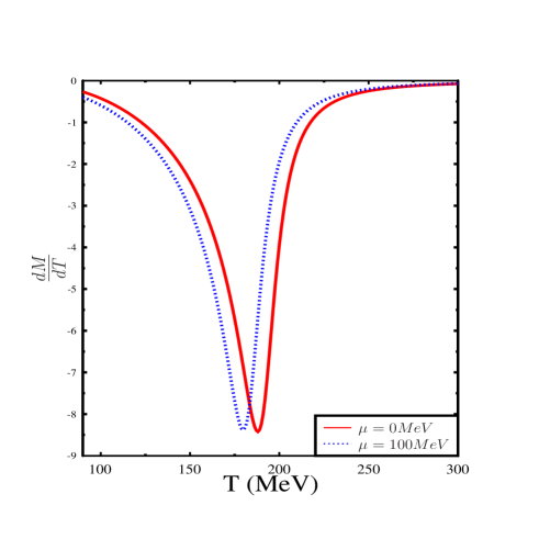
Fig. 1-a	Fig. 1-b

Figure 1: (Fig 1 a) Temperature dependence of the masses of constituent quarks ($M$), and pions ($M_{\pi}$) and sigma mesons ($M_{\sigma}$) for $\mu=0$ and (Fig1-b) temperature derivative of the constituent quark mass for $\mu=0$MeV and $\mu=100$MeV .

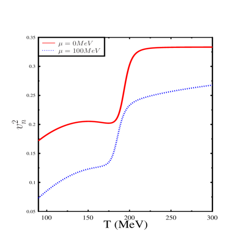
Fig. 2-a	Fig. 2-b

Figure 2: Temperature dependence of square of the velocity of sound ($v_{n}^{2}$) (Fig2-a) and trace anamoly $((\epsilon-3p)/T^{4})$ (Fig 2-b) for $\mu=0$ MeV and $\mu=100$ MeV

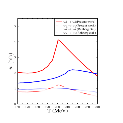
Figure 3: Thermal averaged transition rate shown as a function of temperature. The red curves corresponds to the present calculations while the blue curves correspond to the estimation in Ref. klevanskynpa . The solid and dotted lines correspond to the scattering in the quark- antiquark channels and quark quark channels respectively.

IV Results

The two-flavor NJL model as given in Eq.(1), within which we shall be discussing the results, has three parameters, namely, the four-point coupling $G$, the three-momentum cutoff $\Lambda$ to regularize the integrals appearing in the mass gap equation, and, in the integrals involving meson masses and the current quark mass $m$ that we take to be the same for $u$ and $d$ quarks. Within the mean field approximation for the thermodynamic potential, and the RPA approximation for the meson masses, these three parameters are fixed by fitting the pion mass, the pion decay constant and the quark condensate. While the pion mass $m_{\pi}=135$ MeV mpiexpt and pion decay constant $f_{\pi}=92.4$ MeVfpiexpt are known somewhat accurately, the uncertainties in the quark condensates are rather large. Whereas, the extraction from the QCD sum rules turns out to be in the range 190 MeV$<-\langle\bar{u}u\rangle^{1/3}<$ 260 MeV ( at renormalization scale of 1 GeV) condsum , extraction from lattice simulation turns out to be $-\langle\bar{u}u\rangle^{1/3}\sim 231$ MeV condlat . Here, we have used the parameter set $m=5.6$ MeV, $\Lambda$=587.9 MeV and $G\Lambda^{2}=2.44$. This leads to the vacuum value of the constituent quark mass $M\simeq 400$ MeV, and the condensate value is $-\langle\bar{u}u\rangle^{1/3}=241$ MeV.

Let us first discuss the thermodynamics of the two-flavor NJL model as relevant for the calculation of the transport coefficients.

With the parameters as above, the gap equation is first solved using Eq.(3) for a given temperature and chemical potential. This is then used to solve for the masses of the pion and sigma masses using Eqs.(12) and (13) within the random phase approximation. In Fig.1(a), we have plotted the constituent quark mass, and the meson masses so derived as a function of temperature for $\mu=0$. In the chirally broken phase, the pion mass, being the mass of an approximate Goldstone mode is protected and varies weakly with temperature. On the other hand, the mass of $\sigma$ , which is approximately twice the constituent quark mass, drops significantly near the crossover temperature. At high temperature, being chiral partners, the masses of $\sigma$ and $\pi$ mesons become degenerate and increase linearly with temperature. The constituent quark mass decreases to small values but never vanishes. The chiral crossover transition $T_{\chi}$ turns out to be about 188 MeV for $\mu=0$ and about 180 MeV for $\mu=100$ MeV. These are defined by the peak in the derivative of the constituent mass $(dM/dT)$, which we have shown in Fig.(1b). Let us note here that the constituent mass at $T_{\chi}$ turns out to be about 145 MeV. On the other hand, one can have the other characteristic temperature namely, the Mott temperature $T_{M}$ defined through the relation $m_{\pi}(T_{M})=2M(T_{M})$, i.e., the temperature when the twice the constituent quark mass becomes equal to that of the pion mass. As may be observed in Fig.1-a the Mott temperature for pions is about 197 MeV. This temperature is relevant in the present case where we estimate the relaxation time using quark scattering involving meson exchange.

Next, we show, in Fig 2-a, the temperature dependence of the square of the velocity of sound $v_{n}^{2}=(dp/d\epsilon)_{n}$ at constant quark number density as defined in Eq.(40). The velocity of sound do not show any dip around the critical temperature $T_{\chi}$, but rises around the critical temperature and approaches the value of $\frac{1}{3}$ at high temperatures. In Fig. 2-b , we show the dependence of the trace anomaly $(\epsilon-3p)/T^{4}$. The conformal symmetry is broken maximally at the critical temperature and is larger for higher chemical potential.

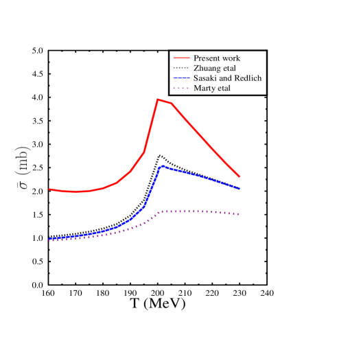
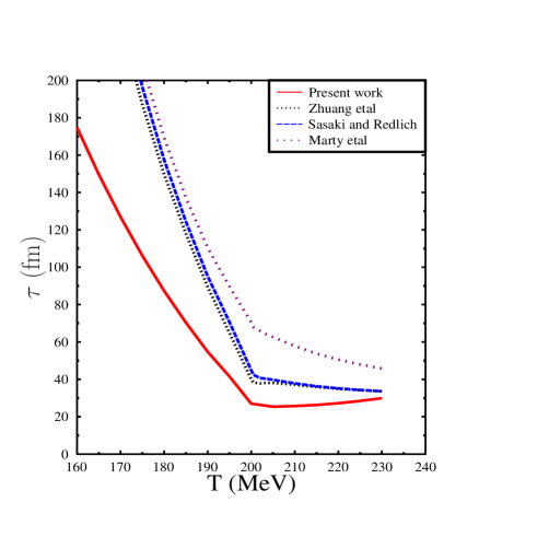
Fig. 4-a	Fig. 4-b

Figure 4: Thermal-average cross section for the process $u\bar{d}\rightarrow u\bar{d}$ as a function of temperature is plotted in Fig 4-a. The present calculation is shown by the solid line. The other results correspond to Zhuang etal klevansky , Sasaki and Redlich sasakinjl and Marty etal marty . In Fig 4-b is plotted the corresponding relaxation time $\tau_{u\bar{d}\rightarrow u\bar{d}}=\bar{\sigma}_{u\bar{d}\rightarrow u\bar{d}}n_{\bar{d}}$.

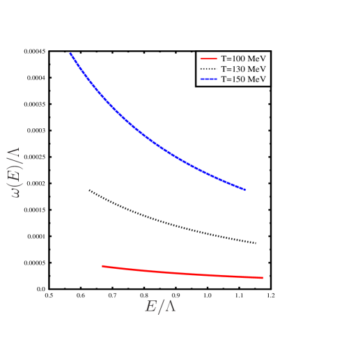
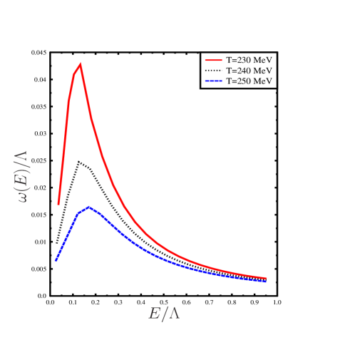
Fig. 5-a	Fig. 5-b

Figure 5: Transition frequency in units of $\Lambda$ for the process $u\bar{d}\rightarrow u\bar{d}$ as a function of function of energy for different temperatures. For temperature less than the Mott temperature is plotted in Fig 5-a while for temperature higher than Mott temperatures is plotted on Fig 5-b.

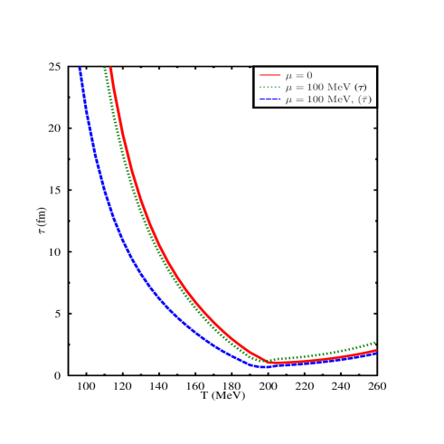
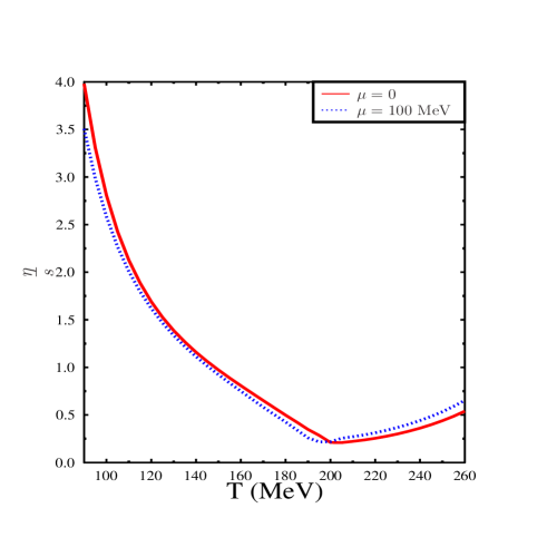
Fig. 6-a	Fig. 6-b

Figure 6: Relaxation time as a function of temperature for $\mu=0$ MeV and for $\mu=100$MeV (Fig 6-a). In Fig (6-b), shear viscosity to entropy density ratio is shown for $\mu=0$ MeV and $\mu=100$ MeV.

We would like to mention that the behavior of the velocity of sound shows a different behavior as compared to lattice simulations tanmoy where it shows a minimum and then rises to a value a little less than the ideal gas limit of $1/3$ . The present results for the sound velocity are similar in nature to linear sigma model calculations of Ref.purnendu with a lighter sigma meson of mass about 600 MeV. This behavior, as we shall observe later, gets reflected in the results for the bulk viscosity.

We then plot the thermal-averaged transition rate $\bar{W}_{ab}$ of Eq.(66) for quark scatterrings for the quark-antiquark chaneel and quark-quark channel in Fig.3. Quark-antiquark scattering turns out to be dominant compared to quark-quark scattering. After thermal averaging the transition rate shows a peak around the Mott transition temperature. Above the Mott temperature, the transition rates decrease with temperature. This one would expect as the meson propagators $D_{M}^{-1}(\sqrt{s},{\bf{0}})\sim\left[(s-\left(m_{M}-i\Gamma/2\right)^{2}\right]$ and both the resonance mass and the width increase with temperature zhuang . The behavior of the transition rate is qualitatively similar to that in Ref. klevanskynpa . The difference could be due to the fact that in Ref. klevanskynpa , where, three-flavors case is considered, there could be more channels possible for quark scattering and also the parameters of the model are different. In the present case, the transition rate decreases faster as compared to Ref klevanskynpa beyond the Mott temperature, leading to a rise of average relaxation time as can be expected from Eq.(73).

A comment regarding estimation of the mean relaxation time may be relevant here, although, ideally one would like to keep the energy-dependent relaxation time and perform the phase space integration in the expression for the transport coefficients. In the present calculations, this is carried out by calculating a mean interaction frequency of the energy dependent interaction frequency related to the standard quantum field theoretic transition rate as in Eqs.(73), (74) and (67). On the other hand, in Ref.s klevansky ; sasakinjl ; marty this averaging is performed by first obtaining an energy averaged cross section e.g. for the process $u,\bar{d}\rightarrow u,\bar{d}$

$$\bar{\sigma}_{u\bar{d}\rightarrow u\bar{d}}(T,\mu)=\int ds\sigma_{u\bar{d}\rightarrow u\bar{d}}(T,\mu)P(s,T,\mu)$$ (77)

where, $P(s,T,\mu)$ is the probability of yielding a quark-antiquark pair with energy $\sqrt{s}$ and is normalized as

$$\int dsP(s,T,\mu)=1.$$ (78)

However, in the three references cited above, the expressions for $P(s,T,\mu)$ are different. In the earliest one klevansky , Zhuang et al take

$$P_{zhuang}(s,T,\mu)=C\sqrt{s(s-4m^{2})}f(\sqrt{s}/2-\mu)f(\sqrt{s}/2+\mu)$$ (79)

while Refs.sasakinjl and marty consider, respectively, the probability function as

$$P_{sas}(s,T,\mu)=C(s-4m^{2})f(\sqrt{s}/2-\mu)f(\sqrt{s}/2+\mu),$$ (80)

$$P_{marty}(s,T,\mu)=C(s-4m^{2})\sqrt{s}f(\sqrt{s}/2-\mu)f(\sqrt{s}/2+\mu).$$ (81)

In Eq.s (79,80,81), the constant $C$ is fixed from the normalization condition of Eq.(78). The contribution of this averaged cross section to the relaxation time is given as

$$\tau_{u\bar{d}\rightarrow u\bar{d}}^{-1}=n_{\bar{d}}\bar{\sigma}_{u\bar{d}\rightarrow u\bar{d}}$$ (82)

The resulting energy-averaged cross section as well as the corresponding relaxation time for the different assumptions for the probability function as compared to the present averaging procedure is shown in Fig.4. The general behavior of the cross section of having a peak around Mott transition is seen all the figures. However, the sharp fall of the cross section beyond the Mott transition is seen with the present averaging while the same for Ref.marty is rather slow. This gets reflected in the behavior of the relaxation time for this process in Fig 4 b. In particular the relaxation time corresponding to Refmarty shows a monotonic decrease beyond the Mott temperature. In this context, it is also relevant to analyze whether the function $\tau(E)$ is reasonably smooth so that the energy averaging is a reasonable approximation. To verify this we also examine the energy-dependent interaction frequency $\omega(E)$ of Eq.(74), which explicitly simplifes to

$$\omega_{a}(E_{a})=\frac{1}{8\pi^{2}E_{a}}\int_{m_{b}}^{\infty}dE_{b}f(E_{b})\int_{-1}^{1}dxW_{ab}(s)$$ (83)

where, –$x=\cos\theta$. To evaluate the above integral, we note that

$$s-(p_{a}+p_{b})^{2}=2E_{a}E_{b}\left(\frac{s}{2E_{a}E_{b}}-y(x)\right)$$ (84)

with

$$y(x)=1+\frac{m_{a}^{2}+m_{b}^{2}}{2E_{a}E_{b}}-\frac{|p_{a}||p_{b}|}{E_{a}E_{b}}x$$ (85)

Inserting the identity involving the delta function

$$1=\int ds\frac{1}{2E_{a}E_{b}}\delta\left(\frac{s}{2E_{a}E_{b}}-y\right)$$ (86)

in the integral Eq.(83), we have

$$\omega(E_{a})=\frac{1}{8\pi^{2}E_{a}}\int dE_{b}p_{b}E_{b}\int dxW_{ab}(s)|_{s=2E_{a}E_{b}(1+\frac{m_{a}^{2}+m_{b}^{2}}{2E_{a}E_{b}}-\frac{|p_{a}||p_{b}|}{E_{a}E_{b}}x)}.$$ (87)

Using Eq.(69) for the transition rate $W_{ab}(s)$, we have calculated the energy-dependent transition frequency $\omega(E_{a})$ for a typical scattering process ($u\bar{d}\rightarrow u\bar{d}$) and have plotted it in Fig 5 a and Fig 5b for temperatures below and above the Mott temperatures respectively. As may be seen the energy dependence of the transition frequency is indeed a smooth function of energy. Below the critical temperature, with an increase in temperature, the interaction frequency increases essentially due to the fact that the sigma meson mass decreases with temperature. This behavior of $\omega(E)$ with energy arising from quark scattering is different from interacting pion gas which diverges at large energy. Indeed, the energy-dependent relaxation time , [inverse of $\omega(E)$] arising from pion scattering shows a peak structure at lower energy as shown in Ref goity . Since pions are not the elementary degrees of freedom in the NJL model, there is no elementary pionic interaction within the model. For different possible behavior of $\omega(E)$ to have finite shear viscosity we refer to Ref.langweise . On the other hand, for temperatures above the Mott temperature, as may be seen in Fig 5 b, the transition frequency weights the lower energy strongly. When the temperature increases, the peak value of $\omega(E)$ is reduced somewhat and the decay from the peak value is slower. The decrease of transition frequency with temperature beyond the Mott temperature is associated with the fact that the meson masses increase with temperature. The rise of the transition frequency at low energies near the Mott temperature also demonstrates the limitation of the approximation of taking an average transition frequency. However, for the estimation of the transport coefficients, this low-energy peak does not make the estimation worse as it is multiplied by a function that itself is suppressed at low momenta as may be seen from expression for e.g. shear viscosity in Eq.(48).

Fig. 7-a	Fig. 7-b

Figure 7: Shear viscosity to entropy ratio for $\mu=0$ for low temperatures (Fig 7-a). The present calculations is shown by the solid lines. The other results correspond to Lang etal lang of interacting pion gas, Fernandez-Fraile and Nicolanicola . The two curves by Kapusta etal from Ref.purnendu correspond to different masses for the sigma mesons. The green dashed curve is for $m_{\sigma}=600$ MeV while the orange dotted curve is with $m_{\sigma}=0.9$ GeV. The pink dot dashed curve is for the SHMC model by Khvorostukhin etal of Refvoskresensky . In Fig. 7-b is shown the ratio for higher temperatures. Present calculations is shown by solid red line, the two curves of Marty etal marty correspond to dynamical quasi particle model (DQPM) and the 3 flavor NJL model, the orange dotted curve by Plumari etal is from Ref. greco , the pink dashed curve by Sasaki etal is for two flavor NJL model of Ref. sasakinjl while the brown dot dashed curve b Lang etal is from Ref.langweise .

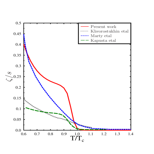
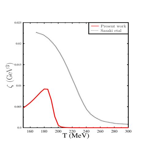
Fig. 8-a	Fig. 8-b

Figure 8: Bulk viscosity to entropy ratio as a function of temperature in units of $T_{c}$ for zero baryon density (8-a). Also shown results from different models, the SHMC model of Khvosthukin etalvoskresensky , Kapusta etal purnendu , the three flavor NJL results of Marty etalmarty . Bulk viscosity in units of GeV³ as a function of temperature is shown in Fig. 8-b. Solid red curve corresponds to the present calculations while dotted curve correspond to the results by Sasaki etal sasakinjl .

Next, with this limitation close to the Mott temperature, we discuss the estimation of averaged relaxation time from all the scatterings in the present approach as a function of temperature. Let us recall that this quantity is inversely related to the transition rate $\bar{W}_{ab}n_{b}$ as in Eq.(73) where $W_{ab}$is the transition rate of all processes with species $a$,$b$ in the the initial states and is related to the corresponding scattering cross section as in Eq.(69). In general, the dominant contribution here comes from quark-antiquark scattering from the $s$ channel through propagation of the resonance states, the pions and the sigma. The mass of the sigma meson decreases with an increase in temperature, becoming a minimum at the Mott transition temperature $T_{M}$ and leading to an enhancement of the cross section. This, in turn, leads to a minimum in the relaxation time. Beyond the transition temperature the resonance masses increase with temperature linearly leading to a smaller cross section and hence an increase in the relaxation time beyond the Mott temperature. This generic feature is observed in Fig.6-a.

Let us note that $\tau^{a}$ depends both on the transition rate and the density of the particles of the initial state other than the species $a$. It turns out that the transition rate is dominant for the process $u\bar{d}\rightarrow u\bar{d}$. At finite chemical potential, for temperatures greater than the transition temperature, quark density is larger compared to the antiquarks. As there are fewer anti quarks to scatter off , the cross section for quark-antiquark scattering decreases leading to $\tau(\mu)>\tau(\mu=0)$. On the other hand, for anti-quarks, there are more quarks to scatter off at nonzero $\mu$ as compared to at $\mu=0$. This leads to a lower value for relaxation time for the antiquark at finite $\mu$ as compared to $\mu=0$ case. On the other hand, for temperatures below the critical temperature, while the quark-antiquark transition rate is dominant, the density of antiquark is suppressed very much by the constituent quark mass for $\mu\neq 0$. The quark number density however is enhanced and the contribution from quark quark scattering becomes more important resulting in a smaller value for the relaxation time at finite $\mu$ compared to the $\mu=0$ case.

At this stage, perhaps it may be relevant to discuss the validity of the Boltzmann kinetic approach that has been used to estimate the transport coefficients within the relaxation time approximation. The same can be a reliable approximation provided the mean free path $\lambda$ is larger than the range $d$. One can define the average mean free path as

$$\lambda_{f}=v_{f}\tau_{f}$$

for a given flavor $f$. . Here the mean velocity $v_{f}$ is given by

$$v_{f}=\frac{2N_{c}}{(2\pi)^{3}n_{f}}\int\frac{d{\bf{p}}}{E_{{\bf{p}}}}|{\bf{p}}|f(E_{{\bf{p}}}).$$ (88)

It turns out that at $T_{Mott}$, $\lambda_{f}=1.2fm$. At the same temperature, the mass of the pion or sigma meson turns out to be about 200 MeV with the corresponding Compton wavelength to be about a Fermi so that the value of the ratio $\lambda/d$ is about 1.2. This ratio is minimal at the Mott temperature and increases rapidly both below and above the Mott temperature. Thus, within the NJL model, it is not too much unreliable to use the Boltzmann equation within the relaxation time approximation except at the Mott transition temperature. Keeping this in mind, we next proceed to estimate the transport coefficients.

In Fig(6-b) we have plotted the shear viscosity to entropy ratio ($\frac{\eta}{s}$) as a function of temperature for $\mu=0$ MeV and $\mu=100$ MeV . As expected from the $\tau$ behavior with temperature, $\eta/s$ has a minimum with $\eta/s|_{min}\sim 0.24$ at the critical temperature beyond which it increases slowly. This behavior of having a minimum around the Mott transition due to the suppression of scattering cross sections at higher temperatures is in contrast to results of Ref.marty where it shows a monotonic decrease with the value of the ratio going below the KSS bound. At finite $\mu$, the ratio $\eta/s$ is larger as compared to vanishing $\mu$. This is due to two reasons. Firstly, $\tau$ at finite $\mu$ is larger and, further, the quark density is also larger as compared to the antiquarks at finite density.

We also compare our results for $\eta/s$ with different existing results for low temperatures below the Mott transition based on different hadronic models for vanishing baryon chemical potential in Fig(7-a). These include results within a interacting pion gas model by Lang etallang , models based on chiral perturbation theory by Fernandez-Fraile and Nicola nicola , linear sigma model within relaxation time approximation purnendu and a hadronic model based on scaling of hadronic masses and couplings (SHMC) by Khvorostukhin etal voskresensky . In general, the behavior of $\eta/s$ seems to be in conformity with these models with the ratio monotonically decreasing with temperature in the range of temperatures considered. In all these models the dominant contributions arise from the pions. The decreasing behavior of the ratio in the present NJL model, on the other hand, arises from the scattering of the constituent quarks exchanging mesons whose mass decreases with temperature leading to a decreasing behavior of the relaxation time. On the other hand, the present estimation of $\eta/s$ overestimates the results of all the models shown in the figure. This could be due to the fact that within the NJL model, the degrees of freedom at these temperatures is a system of constituent quarks rather than pions which should be the dominant physical degrees of freedom. This is also reflected in the behavior of the energy-dependent interaction frequency, which is very different compared to the same due to pion scatteringlangweise ; goity . Apart from this, a somewhat larger value for the ratio within the present model could be due to the small values for the entropy density corresponding to the heavy constituent quarks as compared to the pions.

In Fig. (7-b) we compare our results for $\eta/s$ with those of other models for higher temperatures. In contrast to the results in Ref.s sasakinjl and marty , the ratio does not show a monotonically decreasing behavior. The minimum value value of $\eta/s=0.24$ much above the KSS bound around $T_{Mott}$ and beyond which it increase monotonically. Such a rising behavior with temperature is also seen in two-flavor NJL model using Kubo formalism in Reflangweise .

In Fig. (8-a) we have plotted the specific bulk viscosity normalized to entropy density as a function of temperature. We have also shown here the results of earlier calculations, based on the linear sigma model purnendu , NJL model marty and SHMC model voskresensky . The ratio of bulk viscosity to entropy density increases rapidly near the critical temperature as temperature decrease from high temperature beyond the critical temperature to temperatures below it. However, it is not a maximum at the critical temperature. After the rapid rise near the critical temperature it increases slowly. As may be observed, in all these calculations the ratio $\zeta/s$ decreases monotonically with temperature. We might mention here that, such a behavior of decreasing bulk viscosity to entropy ratio was also observed in estimations based on PHSD transport codes phsdbrat as well as in the linear sigma model in the large N limit dobado . This is in contrast with results in Refs. karschkharzeev ; kharzeevtuchin ; latticemeyer where $\zeta/s$ shows a peak near the critical temperature. On the other hand, we have also plotted the bulk viscosity in units of $GeV^{3}$ in Fig. (8-b) where it shows a maximum around the Mott temperature. Such a feature of a maximum was also seen for the NJL model for two flavors in Ref. sasakinjl . Such a peak in $\zeta$ was also observed in Ref. nicolaprl within a chiral perturbation theory framework with a maximum value of about $\zeta\sim 0.008$ GeV³ as compared to $\zeta\sim 0.01$GeV³ in the NJL model here. However, the ratio $\zeta/s$ does not show such a peak, probably because of the fact that the entropy of the system with massive constituent quarks becomes rather small to mask the peak structure in $\zeta$.

Beyond the Mott transition temperature the ratio $\zeta/s$ vanishes. Let us note that one can rewrite the expression for the bulk viscosity as

$$\zeta = \frac{1}{9T}\sum_{a}\int d\Gamma^{a}\frac{\tau^{a}}{E_{a}^{2}}f_{a}^{0}(1-f_{a}^{0})$$

$$\times \left[{\bf{p}}^{2}(1-3v_{n}^{2})-3v_{n}^{2}\left(M^{2}-TM\frac{dM}{dT}-\mu M\frac{dM}{dT}\right)+3\left(\frac{\partial P}{\partial n}\right)_{\epsilon}\left(M\frac{dM}{\partial\mu}-E_{a}t^{a}\right)\right]^{2}$$

Fig. 9-a	Fig. 9-b

Figure 9: the violation of conformality measure $C_{1}=1-3v_{n}^{2}$ (Fig 9a) and $C_{2}=M^{2}-TM\frac{dM}{dT}$ (Fig 9b) as a function of temperature for $\mu=0$ MeV and for $\mu=100$ MeV

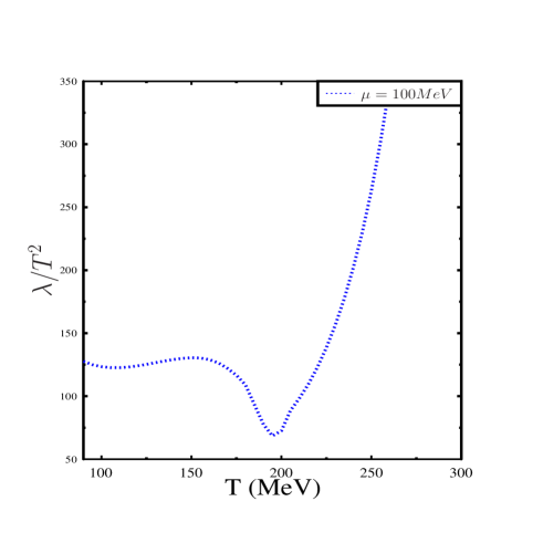
Figure 10: Thermal conductivity($\lambda$) in units of $T^{2}$ for $\mu=100$ MeV.

At zero baryon density, bulk viscosity depends quadratically upon the violation of conformality measures $C_{1}=1-3v_{n}^{2}$ and $C_{2}=M^{2}-TM\frac{dM}{dT}$ purnendu . The behaviors of these two parameters are plotted as a function of temperature in Fig. 9. For comparison, we have also plotted the corresponding quantities at nonzero $\mu$. Both these measures peak where the trace anomaly is maximal as shown in Fig. (2b) As may be observed, $\zeta/s$ is largest when the violation of conformality is large. At finite baryon density, $(1-v_{n}^{2})$ does not vanish, nor does the factor $(\partial P/\partial n)_{\epsilon}$ as a result of which the ratio $\zeta/s$ does not vanish, unlike the $\mu=0$ case. The behavior of bulk viscosity is similar qualitatively to that of linear sigma model of Ref.purnendu . Our results regarding the ratio $\eta/s$ qualitatively look similar as compared to that of Ref.sasakinjl . However, the bulk viscosity to entropy ratio look different as we have implemented the Landau-Lifshitz matching conditions explicitly, leading to a different expression for $\zeta$. Apart from this, while estimating the average relaxation time we have used the transition rate calculated in a covariant manner similar to Ref. klevanskynpa whereas Ref. sasakinjl uses a probability distribution to calculate the thermal-averaged cross section similar to klevansky .

Finally, in Fig. 10 we have plotted thermal conductivity of quark matter at $\mu=100MeV$ in units of $T^{2}$. Let us note that thermal conduction, which involves the relative flow of energy and baryon number, vanishes at zero baryon density. In fact, $\lambda$ diverges as $\lambda\sim 1/n^{2}$ as may be observed in Eq.(65). Such a divergence, however, is inconsequential because, e.g., in the dissipative current as in Eq.(23), it enters as $\lambda n^{2}$ hosoya ; gavin and the heat conduction vanishes for $\mu=0$ daniel . We have therefore shown the results for thermal conductivity for nonvanishing $\mu$ arising from quark scatterings. As may be noted, the ratio $\lambda/T^{2}$ shows a nonmonotonic behavior with a minimum at the critical temperature. The origin of this again is related to the minimum of the relaxation time at the critical temperature. The present behavior is in contrast to the same obtained in Ref. marty , where, the same ratio shows a monotonically decreasing function of temperature. The behavior of $\lambda/T^{2}$ was also studied in Ref.matiello , where, the ratio showed an increasing behavior with temperature with, however, a slower rise with temperature as compared to the results shown in Fig. 6. The reason for a faster rise of $\lambda$ with temperature beyond $T_{mott}$ is two fold. Firstly, the prefactor in Eq.65, $(w/nT)^{2}$, varies at $T^{2}$, because, $w$ rises as $T^{4}$, while $n$ varies as $\mu T^{2}$ in the massless limit for small chemical potential. In addition, at large temperature, the integral itself rises as $T^{3}$ apart from the temperature dependence of relaxation time, which, again is an increasing function of temperature beyond $T_{mott}$. Within the Green-Kubo approach, thermal conductivity was estimated for two flavors using NJL modelfukutome as well as in Ref.nam within the instanton liquid model where however the thermal conductivity saturates beyond T=150 MeV in contrast to the present result.

We may remark here however that, for situations, where, e.g. the pion number is conserved, particularly at low temperatures, heat conductivity can be sustained by pions which themselves have zero baryon number. This is due to the fact that it is possible to have pion scattering in a medium where to number of pions are conserved. This has been the basis of estimating thermal conductivity at zero baryon density nicola ; sourav ; sabyath using chiral perturbation theory. We may note here that, since pions are not the elementary degree of freedom in the NJL model, there is no elementary pion-pion interaction within the model. However, it is possible to construct effective meson-meson interaction using the NJL model considering leading-order diagrams in a $1/N_{c}$ expansion similar to Refs.quack ; heckmann . In such an approach, the pions are coupled through a quark loop as well as exchange of sigma mesons which couple to pions through quark triangles. Such an approach, in principle, can be made to estimate the relaxation time involving pion scattering and hence its contribution to transport coefficients. This is, however, beyond the scope of the present investigation and will be reported elsewhere.

V summary

We have attempted here to compute the transport coefficient in NJL model. The approach uses solving the Boltzmann kinetic equation within relaxation time approximation. To estimate the relaxation time we have considered the quark-antiquark two body scatterrings through exchange of pion and sigma resonances. Since the meson masses are minimal at the transition temperatures beyond which they are degenerate and increase linearly with temperature, the meson propagator occurring in the transition amplitude lead to a large contribution to the cross section for the quark- antiquark scattering. This eventually leads to a smaller relaxation time which, in turn, leads to a minimum in the temperature dependence of the relaxation time. While computing the averaged relaxation time we have performed the procedure in a manifestly covariant manner as in Ref klevanskynpa , rather than multiplying an ad hoc probability function to estimate the thermal-averaged cross section klevansky . We have used the expressions for the transport coefficients that are manifestly positive definite as they should be. The expression for shear viscosity only depends on the relaxation time and the distribution functions. However, the expressions for both the coefficients of bulk viscosity and thermal conductivity involve equation of state. The expressions for the transport coefficients are direct generalization of their counterparts at zero chemical potential albright . All three transport coefficients are minimal at the Mott temperature.

For the estimation of the relaxation time we have only included two-body scatterings. One can generalize this to include decay processes involving the mesons decaying to a pair of quarks and antiquarkslang ; ghoshkrein . We have investigated here the temperature dependence of the transport coefficients in relation to the chiral transition in quark matter. It would be interesting to study the interplay of chiral and deconfinement transition using a Polyakov loop NJL model. Some of these calculations are in progress and will be reported elsewhere.

- (1) U. Heinz and R. Snellings, Annu. Rev. Nucl. Part. Sci. 63, 123-151, 2013
- (2) A. Bstero-Gil, A. Berera and R. Ramos, JCAP1107, 030 (2011).
- (3) H. Heiselberg and C. Pethick,Phys. Rev. D 48, 2916 (1993).
- (4) J. Adams,et al(STAR),Nucl. Phys. A 757, 102 (2005).
- (5) P. Romatschke and U. Romatschke, Phys. Rev. Lett.99,172301, (2007); T. Hirano and M. Gyulassy, Nucl. Phys. A 769, 71, (2006).
- (6) C.Gale, S. Jeon and B. Schenke, International Journal of Modern Physics A 28, 134011,(2013).
- (7) P. Kovtun, D.T. Son and A.O. Starinets, Phys. Rev. Lett.94, 111601, (2005).
- (8) A. Bazavov etal, e-print:arXiv:1407.6387.
- (9) K. Rajagopal and N. Trupuraneni, JHEP1003, 018(2010); J. Bhatt, H. Mishra and V. Sreekanth, JHEP 1011, 106,(2010);ibid Phys. Lett. B704, 486 (2011); ibid Nucl. Phys. A875, 181(2012).
- (10) A. Monnai and T. Hirano, Phys. Rev. C 80, 054906 (2009).
- (11) G. S. Denicol, T. Kodama, T. Koide, and P. Mota, Phys. Rev. C 80, 064901 (2009).
- (12) K. Dusling and T. Schafer, ̵̈ Phys. Rev. C 85, 044909 (2012).
- (13) H. Song and U. Heinz, Phys. Rev. C 81, 024905 (2010).
- (14) J. Noronha-Hostler, G. S. Denicol, J. Noronha, R. P. G. Andrade, and F. Grassi, Phys. Rev. C 88, 044916 (2013); J. Noronha-Hostler, J. Noronha and F. Grassi, Phys. Rev. C 90, 034907 (2014)
- (15) J. B. Rose, J. F. Paquet, G. S. Denicol, M. Luzum, B. Schenke, S. Jeon and C. Gale, Nucl. Phys. A 931, 926 (2014).
- (16) G.S. Denicol, H. Niemi, E. Molnar and D.H. Rischke,Phys. Rev. D 85, 114047 (2012).
- (17) M. Greif, F. Reining, I. Bouras , G.S. Denicol, Z. Xu and C. Greiner, Phys.Rev. E87 ,033019(2013).
- (18) G.S. Denicol, H. Niemi, I. Bouras E. Molnar , Z. Xu , D.H. Rischke, C. Greiner ,Phys. Rev. D 89, 074005 (2014).
- (19) J.I. Kapusta and J.M. Torres-Rincon,Phys. Rev. C 86, 054911 (2012).
- (20) S. Borsonyietal, JHEP1208, 053 (2012).
- (21) R. Kubo,J. Phys. Soc. Jpn. 12,570,(1957).
- (22) C. Sasaki and K.Redlich,Phys. Rev. C 79, 055207 (2009).
- (23) M. Bluhm, B. Kamfer and K. Redlich,Phys. Rev. C 79, 055207 (2009).
- (24) A. Dobado,F.J.Llane-Estrada amd J. Torres Rincon, Phys. Rev. D 79, 055207 (2009).
- (25) P. Chakravarti and J.I. Kapusta Phys. Rev. C 83, 014906 (2011).
- (26) S.Plumari,A. Paglisi,F. Scardina and V. Greco,Phys. Rev. C 83, 054902 (2012)a.
- (27) P. Zhuang,J. Hufner, S.P. Klevansky and L. Neise,Phys. Rev. D 51, 3728 (1995).
- (28) E. Quack, P. Zhuang, Y. Kalinovsky, S.P. Klevansky and J. Hufner,Phys. Lett. B 348, 1 (1995)
- (29) P. Arnold,G.D. Moore and L.G. Yaffe,JHEP, 11, 2000, 001; ibid, JHEP 01 (2003) 030; ibid, JHEP 05 (2003) 051
- (30) M. Bluhm, B. Kamfer and K. Redlich,Phys. Rev. C 84, 025201 (2011).
- (31) Anton Wiranata and Madappa Prakash, Phys. Rev. C 85, , (054908)2012.
- (32) P. Rehberg, S.P. Klevansky and ,J. Hufner,Nucl. Phys. A 608, 356 (1996).
- (33) M. Albright and J.I. Kapusta,Phys. Rev. C 93, 014903 (2016).
- (34) Sabyasachi Ghosh, Phys. Rev. C 90, 025202 (2014); International Journal Of Modern Physics A29, 145005,2014.
- (35) N. Demir and S. A. Bass, Phys. Rev. Lett. 102, 172302 (2009).
- (36) V. Ozvenchuk, O. Linnyk, M. I. Gorenstein, E. L. Bratkovskaya and W. Cassing, Phys. Rev. C 87, 064903 (2013).
- (37) A. Dobado,F.J.Llane-Estrada amd J. Torres Rincon, Phys. Lett. B 702, 43 (2011).
- (38) A.Dobado and J. M. Torres-Rincon Phys. Rev. D 86, 074021 (2012).
- (39) C. Sasaki and K.Redlich,Nucl. Phys. A 832, 62 (2010).
- (40) J.-W. Chen, and E. Nakano, Phys. Lett. B 647, 371 (2007)
- (41) K. Itakura, O. Morimatsu, and H. Otomo, Phys. Rev. D 77, 014014 (2008)
- (42) M.Wang,Y. Jiang, B. Wang, W. Sun and H. Zong, Mod. Phys. lett. A76, 1797,(2011).
- (43) M. Prakash, M. Prakash, , R. Venugopalan and G. Welke,Phys. Rep. 227, 321 (1993).
- (44) D. Fernandiz-Fraile and A. Gomez Nicola, Eur. Phys. J. C 62, 37 (2009).
- (45) S. Matiello, arXiv:1210.1038[hep-ph].
- (46) M. Iwasaki and T. Fukutome, J. Phys. G36, 115012, 2009.
- (47) S. Nam, Mod. Phys. Lett. A 30, 1550054,2015.
- (48) R. Marty, E. Bratkovskaya, W. Cassing, J. Aichelin and H . Berrehrah, Phys. Rev. C 88, 045204 (2013).
- (49) S. Ghosh, Int.J.Mod.Phys. E24 (2015) 07, 1550058
- (50) S. Mitra and S. Sarkar,Phys. Rev. D 89, 054013 (2014).
- (51) A.S. Khvorostukhin, V.D. Toneev and D.N. Voskresensky,Nucl. Phys. A 915, 158 (2013).
- (52) A.S. Khvorostukhin, V.D. Toneev and D.N. Voskresensky, Nucl. Phys. A 845, 106 (2010).
- (53) P. Danielewicz, M. Gyulassy, Phys. Rev. D 31, 53 (1985).
- (54) M. Buballa,Phys. Rep. 407, 205 (2005).
- (55) P. Zhuang,J. Hufner, S.P. Klevansky Nucl. Phys. A 576, 525 (1994).
- (56) Sean Gavin,Nucl. Phys. A 435, 826 (1985).
- (57) A. Hosoya and K. Kajantie ,Nucl. Phys. B 250, 666 (1985).
- (58) S.R. deGroot, W.A. van Leeuwen and Ch. G. van Weert,Relativistic Kinetic Theory: Principles and Applications( North-Holland, Amsterdam, 1980).
- (59) K. Hagiwara et al,Phys. Rev. D 66, 010001 (2002).
- (60) B. Holostein,Phys. Lett. B 244, 83 (1990).
- (61) H.G. Dosch and S. Narrison,Phys. Lett. B 417, 173 (1998).
- (62) L. Giusti,F. Rapuano, M. Talevi and A. Vladikas,Nucl. Phys. B 538, 249 (1999).
- (63) R. Lang, N. Kaiser, W. Weise, Eur. Phys. A48, 109, 2012.
- (64) R. Lang, N. Kaiser, W. Weise, Eur. Phys. A50 , 63, 2014.
- (65) F. Karsch, D. Kharzeev, and K. Tuchin, Phys. Lett. B 663, 217 (2008).
- (66) D. Kharzeev, and K. Tuchin,JHEP 0808,031, (2008).
- (67) H.B. Meyer,Phys. Rev. Lett. 100, 162001 (2008).
- (68) D. Fernandez-Fraile, A. Gomez Nicola, Phys. Rev. Lett. 102, 121601 (2009).
- (69) Sabyasachi Ghosh, Thiago C. Peixoto, Victor Roy, Fernando E. Serna, Gastão Krein e-Print: arXiv:1507.08798 [nucl-th], (2015).
- (70) K. Heckmann, M. Buballa and J. Wambach ,Eur. Phys. J. A 48, 142 (2012)
- (71) J. Edsjo, and P. Gondolo, Phys. Rev. D 56, 1879 (1997).
- (72) J. I. Goity, and H. Leutwyler, Phys. Lett. B 228, 517 (1989).