A Quantum Extended Kalman Filter

Muhammad F. Emzir, Matthew J. Woolley, and Ian R. Petersen School of Engineering and IT , University of New South Wales, ADFA, Canberra, ACT 2600, Australia m.emzir@student.adfa.edu.au
Abstract

A stochastic filter uses a series of measurements over time to produce estimates of unknown variables based on a dynamic model[1]. For a quantum system, such an algorithm is provided by a quantum filter [2], which is also known as a stochastic master equation (SME)[3]. For a linear quantum system subject to linear measurements and Gaussian noise, the quantum filter reduces to a quantum Kalman filter [4, 5].
In this article, we introduce a quantum extended Kalman filter (quantum EKF), which applies a commutative approximation and a time-varying linearization to non-commutative quantum stochastic differential equations (QSDEs). We will show that there are conditions under which a filter similar to the classical EKF can be implemented for quantum systems. The boundedness of estimation errors and the filtering problems with ‘state-dependent’ covariances for process and measurement noises are also discussed.
We demonstrate the effectiveness of the quantum EKF by applying it to systems which involve multiple modes, nonlinear Hamiltonians and simultaneous jump-diffusive measurements.

  • March 2016

1 Introduction

In light of recent advances in quantum engineering, the need to effectively measure and control complex quantum systems has become more crucial. One requirement is to infer unknown observables of a quantum system from noisy measurements based on a dynamic model, a process known as a filtering. The quantum filter was developed in the 1980’s by Belavkin [2, 6, 7, 8]. It has recently been used in experimental systems such as trapped ions [9], cavity QED systems [10], and optomechanical systems [11].
The real-time application of the quantum filter demands an efficient computational algorithm. The quantum filter in the Schrödinger picture, also known as the stochastic master equation, solves the stochastic evolution of the conditional density operator based on the measurement record. In practice, to numerically compute the filter, one has to truncate the Hilbert space basis. The computation time then scales exponentially with the size of the Hilbert space basis which makes the quantum filter difficult to implement in real-time.
In the Heisenberg picture, the quantum filter dynamics reduce to the dynamics of the systems observables 𝐱tsubscript𝐱𝑡\mathbf{x}_{t}. However, for general nonlinear systems, the quantum filter in the Heisenberg picture cannot be interpreted as an explicit solution to the filtering problem [12].
These two facts lead to the need for new approximation techniques. Among these are a Gaussian approximation of the conditional density operator [13, 14]. This work is rather heuristic and lacks an evaluation of the estimation error. Number phase Wigner particle filters have also been suggested[15], but like most particle filter based techniques, they are computationally expensive and not suitable for real-time filtering. Recently a Volterra series approximation [16] was introduced. Although this approach has a tractable error bound [17], estimating the Volterra kernel is complicated in general, and the filter structure is not recursive.
Our approach is to use a commutative operator approximation of the non-commutative nonlinear QSDE. A first order Taylor expansion of the nonlinear quantum Markovian generator is then used to compute the filter gain. We refer to our approach as the quantum extended Kalman filter (quantum EKF), due to the similarity of its structure to the classical extended Kalman filter (EKF). Classical EKF estimation error convergence has been well studied [18, 19, 20, 21, 22], which has resulted in some criteria that guarantee local convergence behavior.
The main difficulty in this approach is that the quantum system, in contrast to a classical system, is governed by a QSDE which involves non-commutative operators. This non-commutativity implies that there is no isomorphism that could map the dynamics into a standard stochastic differential equation (SDE). Due to the non-commutative nature of the QSDE, generally the ordinary partial differentiation with respect to a system observable may not be well defined [23, 24]. Further, the sub-optimality condition of the estimation error has to be defined differently since the system’s observables are operators in Hilbert spaces and not scalar random variables.
In this article, we provide a mathematical description of a quantum EKF. We then establish a sufficient criterion under which the quantum EKF will satisfy a dissipativity condition, which ensures the boundedness of the quadratic estimation error. The cases where the quantum systems and their measurements have a state-dependent covariance, i.e. they are functions of the system observables, are treated as an extension of the quantum EKF. We show that it is sufficient to modify the behavior of the Riccati differential equation to guarantee an equivalent dissipativity condition as the original quantum EKF.
Finally, we demonstrate the application of the quantum EKF to two estimation problems. The first problem is the estimation of quadratures of two cavity modes with Kerr nonlinearities [25] subject to homodyne detection. The second example is the estimation of quadratures of a cavity subject to simultaneous homodyne detection and photon counting measurements.
The readers are referred to [26] for an introduction to quantum probability, quantum stochastic calculus, and quantum non-demolition measurements. We shall use the term ‘classical’ to refer to commutative dynamics and filters. We shall also use the term ‘state-dependent’ covariance to refer to covariance matrices that are functions of the system observables.
The article is organized as follows. The second section will contain some preliminary facts that are used in this article. The main section will describe the main contribution of this work. The first is the mathematical description of the quantum EKF and its existence. The computational complexity of the quantum EKF is analyzed as compared to the SME. Next, we analyze the convergence of the quantum EKF. Lastly, we show an extension of the quantum EKF for state-dependent quantum systems. The third section will be examples of quantum EKF applications, and the last section is the conclusions.

1.1 Notation

Classical probability spaces are denoted by a triple (Ω,,μ)Ω𝜇(\Omega,\mathscr{F},\mu). Plain letters (e.g. P𝑃P) will be used to denote elements of an algebra. \mathbb{P} will be used for a measure from a von Neumann algebra 𝒜𝒜\mathscr{A} to a complex number \mathbb{C}, that is positive and normalized, i.e. (AA)0superscript𝐴𝐴0\mathbb{P}\left(A^{\ast}A\right)\geq 0 and (𝟙)=111\mathbb{P}\left(\mathbb{1}\right)=1. We also use 𝔼(|𝒜)\mathbb{E}_{\mathbb{P}}\left(\cdot|\mathscr{A}\right) to denote a conditional expectation with measure \mathbb{P} with respect to a commutative von Neumann algebra 𝒜𝒜\mathscr{A}. Script face (e.g. \mathscr{H} for Hilbert space) is used to denote a spaces as well as any type of algebra. A class of operators will be denoted by calligraphic face, e.g., for bounded linear operators from a Hilbert space \mathscr{H}, to a Hilbert space 𝒦𝒦\mathscr{K}, we denote (,𝒦)𝒦\mathcal{B}\left(\mathscr{H},\mathscr{K}\right), and also we denote ()(,)\mathcal{B}\left(\mathscr{H}\right)\equiv\mathcal{B}\left(\mathscr{H},\mathscr{H}\right). Bold letters (e.g. 𝐲𝐲\mathbf{y}) will be used to denote a matrix whose elements are operators on a Hilbert space. Hilbert space adjoints, are indicated by , while the complex conjugate transpose will be denoted by \dagger, i.e. (𝐗)=𝐗superscriptsuperscript𝐗topsuperscript𝐗\left(\mathbf{X}^{\ast}\right)^{\top}=\mathbf{X}^{\dagger}. For single-element operators we will use * and \dagger interchangeably. The commutator of 𝐱𝐱\mathbf{x} and 𝐲𝐲\mathbf{y} is given by [𝐱,𝐲]=𝐱𝐲(𝐲𝐱)𝐱𝐲superscript𝐱𝐲topsuperscriptsuperscript𝐲𝐱toptop[\mathbf{x},\mathbf{y}]=\mathbf{x}\mathbf{y}^{\top}-\left(\mathbf{y}\mathbf{x}^{\top}\right)^{\top}, while their anti-commutator is given by {𝐱,𝐲}=𝐱𝐲+(𝐲𝐱)𝐱𝐲superscript𝐱𝐲topsuperscriptsuperscript𝐲𝐱toptop\left\{\mathbf{x},\mathbf{y}\right\}=\mathbf{x}\mathbf{y}^{\top}+\left(\mathbf{y}\mathbf{x}^{\top}\right)^{\top}.

α𝛼\alpha (1)

2 Preliminary

In the classical stochastic case, the optimal nonlinear filter is given by the Kushner-Stratonovich equation [27]. This equation is based on the existence of a sample path, Xtsubscript𝑋𝑡X_{t}, whose dynamics is described by a stochastic differential equation, e.g. dXt=b(Xt)dt+σ(Xt)dWt𝑑subscript𝑋𝑡𝑏subscript𝑋𝑡𝑑𝑡𝜎subscript𝑋𝑡𝑑subscript𝑊𝑡dX_{t}=b(X_{t})dt+\sigma(X_{t})dW_{t}. The nonlinear filter for a function of Xt,f(Xt)subscript𝑋𝑡𝑓subscript𝑋𝑡X_{t},f(X_{t}), is then given via the generator of the Markov process f(Xt)𝑓subscript𝑋𝑡f(X_{t}),

f(Xt)limdt0𝔼[f(Xt+dt)|Xt=x]f(x)dt.𝑓subscript𝑋𝑡subscript𝑑𝑡0𝔼delimited-[]conditional𝑓subscript𝑋𝑡𝑑𝑡subscript𝑋𝑡𝑥𝑓𝑥𝑑𝑡\displaystyle\mathcal{L}f(X_{t})\equiv\lim\limits_{dt\downarrow 0}\dfrac{\mathbb{E}\left[f(X_{t+dt})|X_{t}=x\right]-f(x)}{dt}.

In the nonlinear quantum filter, the sample path of the underlying process Xtsubscript𝑋𝑡X_{t} generally does not exist [26], but instead, we have an equivalent evolution of a unitary operator. By means of the evolution of the unitary operator, for open quantum system with Hamiltonian tsubscript𝑡\mathbb{H}_{t}, and bath coupling operator 𝕃tsubscript𝕃𝑡\mathbb{L}_{t}, the equivalent quantum Markovian generator for a set of observables 𝐱tsubscript𝐱𝑡\mathbf{x}_{t} is given by [28]

(𝐱t)=subscript𝐱𝑡absent\displaystyle\mathcal{L}(\mathbf{x}_{t})= i[𝐱t,t]+12(𝕃t[𝐱t,𝕃t])+12[𝕃t,𝐱t]𝕃t.𝑖Planck-constant-over-2-pisubscript𝐱𝑡subscript𝑡12superscriptsuperscriptsubscript𝕃𝑡superscriptsubscript𝐱𝑡subscript𝕃𝑡toptop12superscriptsuperscriptsubscript𝕃𝑡subscript𝐱𝑡topsubscript𝕃𝑡\displaystyle-\dfrac{i}{\hbar}\left[\mathbf{x}_{t},\mathbb{H}_{t}\right]+\frac{1}{2}\left(\mathbb{L}_{t}^{\dagger}\left[\mathbf{x}_{t},\mathbb{L}_{t}\right]^{\top}\right)^{\top}+\frac{1}{2}\left[\mathbb{L}_{t}^{\ast},\mathbf{x}_{t}\right]^{\top}\mathbb{L}_{t}. (2)

We begin our formulation by considering Hilbert spaces for the system and the environment. First, let the system Hilbert space and the field Boson Fock space, be given by ssubscript𝑠\mathscr{H}_{s} and Γ(𝒽)Γ𝒽\Gamma(\mathscr{h}). The total Hilbert space is given by 𝖳=sΓ(𝒽)subscript𝖳tensor-productsubscript𝑠Γ𝒽\mathscr{H}_{\mathsf{T}}=\mathscr{H}_{s}\otimes\Gamma(\mathscr{h}) and 𝖳[0,t]=sΓ(𝒽)[0,t]subscript𝖳0𝑡tensor-productsubscript𝑠Γsubscript𝒽0𝑡\mathscr{H}_{\mathsf{T}\left[0,t\right]}=\mathscr{H}_{s}\otimes\Gamma(\mathscr{h})_{\left[0,t\right]}. The unitary evolution of the system interaction with the field is described by Ut𝒰(sΓ(𝒽)[0,t])subscript𝑈𝑡𝒰tensor-productsubscript𝑠Γsubscript𝒽0𝑡U_{t}\in\mathcal{U}(\mathscr{H}_{s}\otimes\Gamma(\mathscr{h})_{\left[0,t\right]}), where 𝒰𝒰\mathcal{U} is the class of unitary operators on the associated Hilbert spaces. Let the evolution of a system operator X𝑋X be given by Xt=Ut(X𝟙)Utsubscript𝑋𝑡superscriptsubscript𝑈𝑡tensor-product𝑋1subscript𝑈𝑡X_{t}=U_{t}^{\ast}\left(X\otimes\mathbb{1}\right)U_{t} where 𝟙1\mathbb{1} is identity operator in Γ(𝒽)Γ𝒽\Gamma(\mathscr{h}). Furthermore, without loss of generality, we will assume that the field is initially on the vacuum state. Let the system and field’s initial density operators be given by ρ𝒮(s),ω𝒮(Γ(𝒽))formulae-sequence𝜌𝒮subscript𝑠𝜔𝒮Γ𝒽\rho\in\mathcal{S}(\mathscr{H}_{s})\;,\omega\in\mathcal{S}(\Gamma(\mathscr{h})), where 𝒮𝒮\mathcal{S} is the class of unity trace operator on the associated Hilbert spaces.
The fundamental quantum processes as in [29] are given by d𝐀t,d𝐀t,d𝚲t𝑑superscriptsubscript𝐀𝑡𝑑subscript𝐀𝑡𝑑subscript𝚲𝑡d\mathbf{A}_{t}^{\ast},d\mathbf{A}_{t},d\bm{\Lambda}_{t}, the annihilation, creation and conservation processes. These processes are forward time differential, i.e. d𝐀t,d𝐀t,d𝚲t(𝖳[t,t+δt])𝑑superscriptsubscript𝐀𝑡𝑑subscript𝐀𝑡𝑑subscript𝚲𝑡subscript𝖳𝑡𝑡𝛿𝑡d\mathbf{A}_{t}^{\ast},d\mathbf{A}_{t},d\bm{\Lambda}_{t}\in\mathcal{B}(\mathscr{H}_{\mathsf{T}\left[t,t+\delta t\right]}) and hence commute with 𝐱tsubscript𝐱𝑡\mathbf{x}_{t}. The counting process d𝝀t𝑑subscript𝝀𝑡d\bm{\lambda}_{t} is defined as the diagonal element of d𝚲t𝑑subscript𝚲𝑡d\bm{\Lambda}_{t}. From now on we let (𝖳)subscript𝖳\mathcal{B}\equiv\mathcal{B}\left(\mathscr{H}_{\mathsf{T}}\right) and [t,t+δt](𝖳[t,t+δt])subscript𝑡𝑡𝛿𝑡subscript𝖳𝑡𝑡𝛿𝑡\mathcal{B}_{\left[t,t+\delta t\right]}\equiv\mathcal{B}\left(\mathscr{H}_{\mathsf{T}\left[t,t+\delta t\right]}\right), t](𝖳t])\mathcal{B}_{\left.t\right]}\equiv\mathcal{B}\left(\mathscr{H}_{\mathsf{T}\left.t\right]}\right).
Furthermore, for given system and field initial density operators (ρω)tensor-product𝜌𝜔\left(\rho\otimes\omega\right) there is a corresponding measure \mathbb{P}, called a state, which is positive linear and normalized. For a bounded operator Xt]X\in\mathcal{B}_{t]}, (X)=Tr[Xρω]𝑋Trdelimited-[]tensor-product𝑋𝜌𝜔\mathbb{P}\left(X\right)=\text{Tr}\left[X\rho\otimes\omega\right], see [29, Proposition 9.19].
Let us now fix the von Neumann algebra 𝒩=𝒩\mathscr{N}=\mathcal{B}, and the set of bounded self adjoint operators in total Hilbert space, 𝒪=𝒪(𝖳)𝒩𝒪𝒪subscript𝖳𝒩\mathcal{O}=\mathcal{O}\left(\mathscr{H}_{\mathsf{T}}\right)\subset\mathscr{N}. We denote 𝐱t𝒪tsubscript𝐱𝑡subscript𝒪𝑡\mathbf{x}_{t}\in\mathcal{O}_{t} to be a set of system observables evolved up to time t𝑡t.
In the quantum probability setting, a quantum probability space is defined by specifying a von Neumann algebra 𝒩𝒩\mathscr{N} and a state \mathbb{P}. Let 𝒜𝒩𝒜𝒩\mathscr{A}\subset\mathscr{N} be a commutative von Neumann sub algebra. We call the set 𝒜={B𝒩:AB=BA,A𝒜}superscript𝒜conditional-set𝐵𝒩formulae-sequence𝐴𝐵𝐵𝐴for-all𝐴𝒜\mathscr{A}^{\prime}=\left\{B\in\mathscr{N}:AB=BA,\;\forall A\in\mathscr{A}\right\} the commutant of 𝒜𝒜\mathscr{A} in 𝒩𝒩\mathscr{N}. The conditional expectation in the quantum probability setting is defined as follows.

Definition 2.1.

[26] For a given quantum probability space (𝒩,)𝒩\left(\mathscr{N},\mathbb{P}\right), let 𝒜𝒩𝒜𝒩\mathscr{A}\subset\mathscr{N} be a commutative von Neumann sub-algebra. Then the map 𝔼[|𝒜]:𝒜𝒜\mathbb{E}_{\mathbb{P}}\left[\left.\cdot\right|\mathscr{A}\right]:\mathscr{A}^{\prime}\rightarrow\mathscr{A} is called the conditional expectation from 𝒜superscript𝒜\mathscr{A}^{\prime} onto 𝒜𝒜\mathscr{A} if (𝔼[B|𝒜]A)=(BA),A𝒜,B𝒜formulae-sequencesubscript𝔼delimited-[]conditional𝐵𝒜𝐴𝐵𝐴formulae-sequencefor-all𝐴𝒜𝐵superscript𝒜\mathbb{P}\left(\mathbb{E}_{\mathbb{P}}\left[\left.B\right|\mathscr{A}\right]A\right)=\mathbb{P}\left(BA\right),\;\forall A\in\mathscr{A},\;B\in\mathscr{A}^{\prime}.

The following theorem is fundamental to obtain the relation between quantum probability and the classical Kolmogorov probability axioms. In addition, we will use this theorem to show the implementation of the quantum EKF as a classical EKF in the following section. The proof of the theorem is given in [30, §1.1.8][26].

Theorem 2.1.

Let 𝒜𝒜\mathscr{A} be a commutative von Neumann algebra. Then 𝒜𝒜\mathscr{A} is \ast-isomorphic to (Ω,,μ)superscriptΩ𝜇\mathcal{L}^{\infty}\left(\Omega,\mathscr{F},\mu\right), with \ast-isomorphism τ𝜏\tau. Furthermore, a normal state \mathbb{P} on 𝒜𝒜\mathscr{A} defines a probability measure μPsubscript𝜇𝑃\mu_{P}, which is absolutely continuous with respect to μ𝜇\mu, such that, (A)=𝔼μP(τ(A))𝐴subscript𝔼subscript𝜇𝑃𝜏𝐴\mathbb{P}\left(A\right)=\mathbb{E}_{\mu_{P}}\left(\tau\left(A\right)\right), for all A𝒜𝐴𝒜A\in\mathscr{A}.

We notice here that the commutative von Neumann algebra 𝒜𝒜\mathscr{A} corresponds to a classical field \mathscr{F}, and every projection operator in 𝒜𝒜\mathscr{A} corresponds to a classical event.
In the following discussion, we will use delimited-∥∥\left\lVert\cdot\right\rVert the following semi-norm on \mathcal{B}: if 𝐱n×1𝐱superscript𝑛1\mathbf{x}\in\mathcal{B}^{n\times 1}, then

𝐱(𝐱𝐱)12.delimited-∥∥𝐱superscriptsuperscript𝐱𝐱12\left\lVert\mathbf{x}\right\rVert\equiv{\mathbb{P}\left(\mathbf{x}^{\dagger}\mathbf{x}\right)}^{\frac{1}{2}}. (3)

This quantity is not a norm since, (𝐱𝐱)superscript𝐱𝐱\mathbb{P}\left(\mathbf{x}^{\dagger}\mathbf{x}\right) can be zero for non zero 𝐱𝐱\mathbf{x} that is perpendicular to the density operator. Furthermore, a partial order of two operators, A>B𝐴𝐵A>B is taken in the sense of \mathbb{P}, where A>B𝐴𝐵A>B in \mathbb{P} denotes (AB)>0𝐴𝐵0\mathbb{P}\left(A-B\right)>0. Now suppose we have two operator vectors 𝐱𝒜,𝐱^𝒜formulae-sequence𝐱superscript𝒜^𝐱𝒜\mathbf{x}\in\mathscr{A}^{\prime},\hat{\mathbf{x}}\in\mathscr{A}, where 𝒜𝒜\mathscr{A} is a commutative von Neumann algebra. Under semi-norm(3), by Definition 2.1, we obtain

𝐱𝐱^=((𝐱𝐱^)(𝐱𝐱^))1/2=(𝔼[(𝐱𝐱^)(𝐱𝐱^)|𝒜])1/2.delimited-∥∥𝐱^𝐱superscriptsuperscript𝐱^𝐱𝐱^𝐱12superscriptsubscript𝔼delimited-[]conditionalsuperscript𝐱^𝐱𝐱^𝐱𝒜12\left\lVert\mathbf{x}-\hat{\mathbf{x}}\right\rVert=\mathbb{P}\left(\left(\mathbf{x}-\hat{\mathbf{x}}\right)^{\dagger}\left(\mathbf{x}-\hat{\mathbf{x}}\right)\right)^{1/2}=\mathbb{P}\left(\mathbb{E}_{\mathbb{P}}\left[\left.\left(\mathbf{x}-\hat{\mathbf{x}}\right)^{\dagger}\left(\mathbf{x}-\hat{\mathbf{x}}\right)\right|\mathscr{A}\right]\right)^{1/2}. (4)

The last equation implies that, for any ϵ>0italic-ϵ0\epsilon>0, {ω:𝐱𝐱^<ϵ}𝒜conditional-set𝜔delimited-∥∥𝐱^𝐱italic-ϵ𝒜\left\{\omega:\left\lVert\mathbf{x}-\hat{\mathbf{x}}\right\rVert<\epsilon\right\}\in\mathscr{A}. That is, the event that 𝐱𝐱^<ϵdelimited-∥∥𝐱^𝐱italic-ϵ\left\lVert\mathbf{x}-\hat{\mathbf{x}}\right\rVert<\epsilon is 𝒜limit-from𝒜\mathscr{A}- measurable. Later on we will use this fact to define a Markov time when we are dealing with the stochastic stability of the quantum EKF, see Section 3.3.
For a self adjoint element T𝒩𝑇𝒩T\in\mathscr{N} there is a -isomorphism ff(T)𝑓𝑓𝑇f\rightarrow f(T) from a continuous function in the spectrum of T𝑇T, IT=sp(T)subscript𝐼𝑇𝑠𝑝𝑇I_{T}=sp(T)\in\mathbb{R}, namely 𝒞(IT)𝒞subscript𝐼𝑇\mathcal{C}(I_{T}), onto the 𝒞superscript𝒞\mathcal{C}^{\ast}-subalgebra 𝒞(T)superscript𝒞𝑇\mathcal{C}^{\ast}(T) of 𝒩𝒩\mathscr{N} generated by T𝑇T and the identity element 𝟙1\mathbb{1}.
The following two propositions show how one can define a partial derivative for an operator differentiable mappings which will be used in the filter algorithm. Both have been proved in [31, 32], but we mention the proof here again for the sake of completeness. For the two propositions, we will recall the following definitions,

Definition 2.2.

[33, 31]If 𝒳𝒳\mathscr{X} and 𝒴𝒴\mathscr{Y} are Banach spaces with norm 𝒳subscriptdelimited-∥∥𝒳\left\lVert\cdot\right\rVert_{\mathscr{X}} and 𝒴subscriptdelimited-∥∥𝒴\left\lVert\cdot\right\rVert_{\mathscr{Y}} respectively, a mapping f:𝒟𝒴:𝑓𝒟𝒴f:\mathscr{D}\rightarrow\mathscr{Y} on a subset 𝒟𝒟\mathscr{D} of 𝒳𝒳\mathscr{X} is Fréchet differentiable at T𝒟𝑇𝒟T\in\mathscr{D} if there is a bounded linear operator D(f,T)subscript𝐷𝑓𝑇D_{\left(f,T\right)} in (𝒳,𝒴)𝒳𝒴\mathcal{B}\left(\mathscr{X},\mathscr{Y}\right), the class of linear bounded functions from 𝒳𝒳\mathscr{X} to 𝒴𝒴\mathscr{Y}, such that,

limS0f(T+S)f(T)D(f,T)S𝒴S𝒳=0.subscript𝑆0subscriptdelimited-∥∥𝑓𝑇𝑆𝑓𝑇subscript𝐷𝑓𝑇𝑆𝒴subscriptdelimited-∥∥𝑆𝒳0\lim\limits_{S\rightarrow 0}\dfrac{\left\lVert f(T+S)-f(T)-D_{\left(f,T\right)}S\right\rVert_{\mathscr{Y}}}{\left\lVert S\right\rVert_{\mathscr{X}}}=0. (5)

If D(f,T)subscript𝐷𝑓𝑇D_{\left(f,T\right)} is defined for every T𝒳𝑇𝒳T\in\mathscr{X}, then f𝑓f is Fréchet differentiable on 𝒟𝒟\mathscr{D}.

Definition 2.3.

[31] Let 𝒰𝒰\mathscr{U} be any unitary C-* algebra, and 𝒮𝒮\mathscr{S} is the corresponding self adjoint sub-algebra. For any continuous function f𝑓f on the compact interval I𝐼I, f𝒞(I)𝑓𝒞𝐼f\in\mathcal{C}\left(I\right) is said to be operator differentiable if the operator function

f:𝒮I𝒰,:𝑓superscript𝒮𝐼𝒰\displaystyle f:\mathscr{S}^{I}\rightarrow\mathscr{U},

is Fréchet differentiable on 𝒟=𝒮I𝒟superscript𝒮𝐼\mathscr{D}=\mathscr{S}^{I}, symbolically f𝒞op1(I)𝑓subscriptsuperscript𝒞1𝑜𝑝𝐼f\in\mathcal{C}^{1}_{op}(I).

Proposition 2.1.

[32, 31] If f𝒞op1(I)𝑓subscriptsuperscript𝒞1𝑜𝑝𝐼f\in\mathcal{C}^{1}_{op}(I), then f𝒞1(I)𝑓superscript𝒞1𝐼f\in\mathcal{C}^{1}\left(I\right)

Proof.

Without losing of generality, we may assume that I𝐼I is bounded, i.e I={x:aib}𝐼conditional-set𝑥𝑎𝑖𝑏I=\left\{x\in\mathbb{R}:a\leq i\leq b\right\}, and f:𝒰𝒰:𝑓𝒰𝒰f:\mathscr{U}\rightarrow\mathscr{U}. Set 𝒰=𝒞b(I)𝒰subscript𝒞𝑏𝐼\mathscr{U}=\mathcal{C}_{b}\left(I\right), the set of a bounded continuous functions on I𝐼I. Since f𝒞op1(I)𝑓subscriptsuperscript𝒞1𝑜𝑝𝐼f\in\mathcal{C}^{1}_{op}(I), the differentiability of f𝑓f at a function g𝒰𝑔𝒰g\in\mathscr{U} implies that for every ϵ>0italic-ϵ0\epsilon>0, there exists δ>0𝛿0\delta>0 such that for any function h,h<δdelimited-∥∥𝛿h,\left\lVert h\right\rVert<\delta

f(g+h)f(g)D(f,g)hϵh,delimited-∥∥𝑓𝑔𝑓𝑔subscript𝐷𝑓𝑔italic-ϵdelimited-∥∥\left\lVert f(g+h)-f(g)-D_{\left(f,g\right)}h\right\rVert\leq\epsilon\left\lVert h\right\rVert, (6)

which shows that, D(f,g)h:h(fg)h:subscript𝐷𝑓𝑔superscript𝑓𝑔D_{\left(f,g\right)}h:h\rightarrow\left(f^{\prime}\circ g\right)h. Suppose there exist two arbitrary points x1,x0Isubscript𝑥1subscript𝑥0𝐼x_{1},x_{0}\in I, satisfying |x1x0|<δsubscript𝑥1subscript𝑥0𝛿\left|x_{1}-x_{0}\right|<\delta. Now let g(x)𝑔𝑥g(x) equal the identity function, and h(x)=x0x1𝑥subscript𝑥0subscript𝑥1h(x)=x_{0}-x_{1} constant. We get, h<δdelimited-∥∥𝛿\left\lVert h\right\rVert<\delta, and at x=x1𝑥subscript𝑥1x=x_{1},

f(x1+x0x1)f(x1)f(x1)(x0x1)=f(x0)f(x1)f(x1)(x0x1).𝑓subscript𝑥1subscript𝑥0subscript𝑥1𝑓subscript𝑥1superscript𝑓subscript𝑥1subscript𝑥0subscript𝑥1𝑓subscript𝑥0𝑓subscript𝑥1superscript𝑓subscript𝑥1subscript𝑥0subscript𝑥1f(x_{1}+x_{0}-x_{1})-f(x_{1})-f^{\prime}\left(x_{1}\right)(x_{0}-x_{1})=f(x_{0})-f(x_{1})-f^{\prime}\left(x_{1}\right)(x_{0}-x_{1}).

Next interchanging x0subscript𝑥0x_{0} and x1subscript𝑥1x_{1}, we get,

f(x1)f(x0)f(x0)(x1x0).𝑓subscript𝑥1𝑓subscript𝑥0superscript𝑓subscript𝑥0subscript𝑥1subscript𝑥0f(x_{1})-f(x_{0})-f^{\prime}\left(x_{0}\right)(x_{1}-x_{0}).

Adding this and the previous equation, and dividing by x1x0delimited-∥∥subscript𝑥1subscript𝑥0\left\lVert x_{1}-x_{0}\right\rVert, we get

f(x0)f(x1)<ϵdelimited-∥∥superscript𝑓subscript𝑥0superscript𝑓subscript𝑥1italic-ϵ\left\lVert f^{\prime}\left(x_{0}\right)-f^{\prime}\left(x_{1}\right)\right\rVert<\epsilon

which shows the continuity of fsuperscript𝑓f^{\prime} on I𝐼I. ∎

Proposition 2.2.

[31] If f𝒞op1(I)𝑓subscriptsuperscript𝒞1𝑜𝑝𝐼f\in\mathcal{C}^{1}_{op}(I), for any two elements S,T𝒰𝑆𝑇𝒰S,T\in\mathscr{U}, a unital commutative C- algebra, then

D(f,T)S=f(T)S.subscript𝐷𝑓𝑇𝑆superscript𝑓𝑇𝑆\displaystyle D_{\left(f,T\right)}S=f^{\prime}(T)S.
Proof.

Let S,T𝒰𝑆𝑇𝒰S,T\in\mathscr{U}, a unital commutative C- algebra on the space 𝒳𝒳\mathscr{X}. We write, f(T)(x)=f(T(x)),x𝒳formulae-sequence𝑓𝑇𝑥𝑓𝑇𝑥for-all𝑥𝒳f(T)(x)=f(T(x)),\forall x\in\mathscr{X}, so that, as the previous proposition, f(T)=fT𝑓𝑇𝑓𝑇f(T)=f\circ T. Since f𝒞op1(I)𝑓subscriptsuperscript𝒞1𝑜𝑝𝐼f\in\mathcal{C}^{1}_{op}(I), by definition, there exists a differential DTf(𝒰,𝒰)subscript𝐷𝑇𝑓𝒰𝒰D_{T}f\in\mathcal{B}\left(\mathscr{U},\mathscr{U}\right), such that,

f(T+ϵS)(x)=f(T)(x)+ϵD(f,T)S(x)+ϵRϵ(x),𝑓𝑇italic-ϵ𝑆𝑥𝑓𝑇𝑥italic-ϵsubscript𝐷𝑓𝑇𝑆𝑥italic-ϵsubscript𝑅italic-ϵ𝑥f(T+\epsilon S)(x)=f(T)(x)+\epsilon D_{\left(f,T\right)}S(x)+\epsilon R_{\epsilon}(x), (7)

where limϵ0Rϵ=0subscriptitalic-ϵ0subscript𝑅italic-ϵ0\lim\limits_{\epsilon\rightarrow 0}R_{\epsilon}=0. By Proposition 2.1, it follows that,

D(f,T)S(x)=f(T(x))S(x),subscript𝐷𝑓𝑇𝑆𝑥superscript𝑓𝑇𝑥𝑆𝑥D_{\left(f,T\right)}S(x)=f^{\prime}(T(x))S(x),

as desired. ∎

By definition the last proposition is also true for a commutative von Neumann algebra, since any von Neumann algebra is a C- subalgera of ()\mathcal{B}\left(\mathscr{H}\right) that is strongly closed and contains the identity, for \mathscr{H} is any Hilbert space [34].
The condition that 𝒰𝒰\mathscr{U} is commutative in Proposition 2.2 is essential. In addition, it was proven that one can construct a 𝒞1superscript𝒞1\mathcal{C}^{1} function that is not operator differentiable [35]. Moreover, if f𝒞2𝑓superscript𝒞2f\in\mathcal{C}^{2}, then its extension is operator differentiable, see [36, 37]. Hence 𝒞2𝒞op1𝒞1superscript𝒞2superscriptsubscript𝒞𝑜𝑝1superscript𝒞1\mathcal{C}^{2}\subseteq\mathcal{C}_{op}^{1}\subseteq\mathcal{C}^{1}.

Definition 2.4.

An operator A𝐴A in a Hilbert space \mathscr{H} is single valued, if it can be written as a scalar times an identity,

A=a𝟙,a.formulae-sequence𝐴𝑎1𝑎\displaystyle A=a\mathbb{1},a\in\mathbb{C}. (8)

A matrix 𝐀𝐀\mathbf{A} whose each elements are operators in \mathscr{H} is single valued if each element of 𝐀𝐀\mathbf{A} is single valued.

3 Main Statement

3.1 Extended Kalman filter for a class of open quantum quantum systems with diffusive and Poissonian measurements

Let 𝒢𝒢\mathcal{G} be an m𝑚m channel open quantum system with parameters (𝕊,𝕃,)𝕊𝕃(\mathbb{S},\mathbb{L},\mathbb{H}), 𝕊m×m,𝕃tm×1,𝒪tm×1formulae-sequence𝕊superscript𝑚𝑚formulae-sequence𝕃superscriptsubscript𝑡𝑚1superscriptsubscript𝒪𝑡𝑚1\mathbb{S}\in\mathbb{C}^{m\times m},\mathbb{L}\in\mathcal{B}_{t}^{m\times 1},\mathbb{H}\in\mathcal{O}_{t}^{m\times 1} and 𝕊𝕊=𝕊𝕊=𝐈𝕊superscript𝕊superscript𝕊𝕊𝐈\mathbb{S}\mathbb{S}^{\dagger}=\mathbb{S}^{\dagger}\mathbb{S}=\mathbf{I}. The class of open quantum system that we consider here is the one which has covariance matrices independent of 𝐱tsubscript𝐱𝑡\mathbf{x}_{t}. A more general class of open quantum system with state-dependent covariances will be considered in the following section. The smallest von Neumann algebra generated from the measurement up to time t𝑡t is given by 𝒴tsubscript𝒴𝑡\mathscr{Y}_{t}. As in the classical setting, we can always assume that the von Neumann algebra 𝒴tsubscript𝒴𝑡\mathscr{Y}_{t} is right continuous, by taking 𝒴t=𝒴t+=s>t𝒴tsubscript𝒴𝑡subscript𝒴subscript𝑡subscript𝑠𝑡subscript𝒴𝑡\mathscr{Y}_{t}=\mathscr{Y}_{t_{+}}=\bigcap_{s>t}\mathscr{Y}_{t} [38].
We assume that the scattering matrix 𝕊𝕊\mathbb{S} is single valued. This implies that for any Xt=UtXUtsubscript𝑋𝑡superscriptsubscript𝑈𝑡𝑋subscript𝑈𝑡X_{t}=U_{t}^{\dagger}XU_{t}, Tr[((𝕊Xt𝕊)Xt)d𝚲t]=0Trdelimited-[]superscript𝕊subscript𝑋𝑡𝕊subscript𝑋𝑡𝑑superscriptsubscript𝚲𝑡top0\text{Tr}\left[((\mathbb{S}^{\dagger}X_{t}\mathbb{S})-X_{t})d\bm{\Lambda}_{t}^{\top}\right]=0. This ensures that the open quantum system evolution can be described by a diffusive QSDE as follows[39]: {dgroup}

d𝐱t=𝐟(𝐱t)dt+𝐆(𝐱t)d𝐀t+𝐆(𝐱t)d𝐀t,𝑑subscript𝐱𝑡𝐟subscript𝐱𝑡𝑑𝑡𝐆subscript𝐱𝑡𝑑superscriptsubscript𝐀𝑡𝐆superscriptsubscript𝐱𝑡𝑑subscript𝐀𝑡d\mathbf{x}_{t}=\mathbf{f}(\mathbf{x}_{t})dt+\mathbf{G}(\mathbf{x}_{t})d\mathbf{A}_{t}^{\ast}+\mathbf{G}(\mathbf{x}_{t})^{\ast}d\mathbf{A}_{t}, (9)
{dsuspend}

with,

𝐟(𝐱t)=(𝐱t),𝐟subscript𝐱𝑡subscript𝐱𝑡\mathbf{f}(\mathbf{x}_{t})=\mathcal{L}(\mathbf{x}_{t}),
𝐆(𝐱t)=[𝐱t,𝕃t]𝕊t.𝐆subscript𝐱𝑡subscript𝐱𝑡subscript𝕃𝑡superscriptsubscript𝕊𝑡\mathbf{G}(\mathbf{x}_{t})=\left[\mathbf{x}_{t},\mathbb{L}_{t}\right]\mathbb{S}_{t}^{\ast}.

We shall assume that the number of measurements subject to the open quantum system 𝒢𝒢\mathcal{G} also equal to m𝑚m. The class of measurements of the quantum system above are assumed to be a collection of m𝑚m functions of output field creation, annihilation, and conservation processes, as below {dgroup}

d𝐲t=𝐄td𝐀~t+𝐄td𝐀~t+𝐍td𝝀~t,𝑑subscript𝐲𝑡subscript𝐄𝑡𝑑superscriptsubscript~𝐀𝑡subscriptsuperscript𝐄𝑡𝑑subscript~𝐀𝑡subscript𝐍𝑡𝑑subscript~𝝀𝑡d\mathbf{y}_{t}=\mathbf{E}_{t}d\tilde{\mathbf{A}}_{t}^{\ast}+\mathbf{E}^{\ast}_{t}d\tilde{\mathbf{A}}_{t}+\mathbf{N}_{t}d\tilde{\bm{\lambda}}_{t}, (10)
{dsuspend}

where,

d𝝀~t=diag(d𝚲~t),𝑑subscript~𝝀𝑡diag𝑑subscript~𝚲𝑡d\tilde{\bm{\lambda}}_{t}=\text{diag}\left(d\tilde{\bm{\Lambda}}_{t}\right),
d𝐀~t=𝕊td𝐀t+𝕃tdt,𝑑subscript~𝐀𝑡subscript𝕊𝑡𝑑subscript𝐀𝑡subscript𝕃𝑡𝑑𝑡d\tilde{\mathbf{A}}_{t}=\mathbb{S}_{t}d\mathbf{A}_{t}+\mathbb{L}_{t}dt,
d𝚲~t=𝕊td𝚲𝕊t+𝕊td𝐀t𝕃t+𝕃td𝐀t𝕊t+𝕃𝕃dt.𝑑subscript~𝚲𝑡superscriptsubscript𝕊𝑡𝑑𝚲superscriptsubscript𝕊𝑡topsuperscriptsubscript𝕊𝑡𝑑superscriptsubscript𝐀𝑡superscriptsubscript𝕃𝑡topsuperscriptsubscript𝕃𝑡𝑑superscriptsubscript𝐀𝑡topsuperscriptsubscript𝕊𝑡topsuperscript𝕃superscript𝕃top𝑑𝑡d\tilde{\bm{\Lambda}}_{t}=\mathbb{S}_{t}^{*}d\bm{\Lambda}\mathbb{S}_{t}^{\top}+\mathbb{S}_{t}^{*}d\mathbf{A}_{t}^{\ast}\mathbb{L}_{t}^{\top}+\mathbb{L}_{t}^{\ast}d\mathbf{A}_{t}^{\top}\mathbb{S}_{t}^{\top}+\mathbb{L}^{\ast}\mathbb{L}^{\top}dt.

To satisfy the non-demolition and self-nondemolition properties, 𝐄tsubscript𝐄𝑡\mathbf{E}_{t} and 𝐍tsubscript𝐍𝑡\mathbf{N}_{t} have to satisfy the algebraic condition in Theorem 3.1 of [12]. We could then simplify (10) to

d𝐲t=𝑑subscript𝐲𝑡absent\displaystyle d\mathbf{y}_{t}= 𝐡(𝐱t)dt+𝐋(𝐱t)d𝐀t+𝐋(𝐱t)d𝐀t+𝐍td𝜶t,𝐡subscript𝐱𝑡𝑑𝑡𝐋subscript𝐱𝑡𝑑superscriptsubscript𝐀𝑡𝐋superscriptsubscript𝐱𝑡𝑑subscript𝐀𝑡subscript𝐍𝑡𝑑subscript𝜶𝑡\displaystyle\mathbf{h}(\mathbf{x}_{t})dt+\mathbf{L}(\mathbf{x}_{t})d\mathbf{A}_{t}^{\ast}+\mathbf{L}(\mathbf{x}_{t})^{\ast}d\mathbf{A}_{t}+\mathbf{N}_{t}d\bm{\alpha}_{t}, (11a)
𝐡(𝐱t)=𝐡subscript𝐱𝑡absent\displaystyle\mathbf{h}(\mathbf{x}_{t})= 𝐄t𝕃t+𝐄t𝕃t+𝐍t𝐥t,subscriptsuperscript𝐄𝑡subscript𝕃𝑡subscript𝐄𝑡superscriptsubscript𝕃𝑡subscript𝐍𝑡subscript𝐥𝑡\displaystyle\mathbf{E}^{\ast}_{t}\mathbb{L}_{t}+\mathbf{E}_{t}\mathbb{L}_{t}^{\ast}+\mathbf{N}_{t}\mathbf{l}_{t}, (11b)
𝐋(𝐱t)=𝐋subscript𝐱𝑡absent\displaystyle\mathbf{L}(\mathbf{x}_{t})= (𝐄t+𝐍t𝕃¯)𝕊t,subscript𝐄𝑡subscript𝐍𝑡¯𝕃superscriptsubscript𝕊𝑡\displaystyle\left(\mathbf{E}_{t}+\mathbf{N}_{t}\bar{\mathbb{L}}\right)\mathbb{S}_{t}^{*}, (11c)

where 𝐍t𝒪m×msubscript𝐍𝑡superscript𝒪𝑚𝑚\mathbf{N}_{t}\in\mathcal{O}^{m\times m}, and {dgroup*}

𝕃¯=[𝕃1,t00𝕃i,t00𝕃m,t],𝐥t=[𝕃1,t𝕃1,t𝕃m,t𝕃m,t],d𝜶t=diag(𝕊td𝚲𝕊t).formulae-sequence¯𝕃matrixsubscript𝕃1𝑡missing-subexpressionmissing-subexpression00missing-subexpressionsubscript𝕃𝑖𝑡missing-subexpression00missing-subexpressionmissing-subexpressionsubscript𝕃𝑚𝑡formulae-sequencesubscript𝐥𝑡matrixsuperscriptsubscript𝕃1𝑡subscript𝕃1𝑡superscriptsubscript𝕃𝑚𝑡subscript𝕃𝑚𝑡𝑑subscript𝜶𝑡diagsuperscriptsubscript𝕊𝑡𝑑𝚲superscriptsubscript𝕊𝑡top{\bar{\mathbb{L}}=\begin{bmatrix}\mathbb{L}_{1,t}&&\cdots&&0\\ 0&&\mathbb{L}_{i,t}&&0\\ 0&&\cdots&&\mathbb{L}_{m,t}\\ \end{bmatrix}},{\mathbf{l}_{t}=\begin{bmatrix}\mathbb{L}_{1,t}^{\ast}\mathbb{L}_{1,t}\\ \vdots\\ \mathbb{L}_{m,t}^{\ast}\mathbb{L}_{m,t}\\ \end{bmatrix}},\\ {d\bm{\alpha}_{t}=\text{diag}\left(\mathbb{S}_{t}^{*}d\bm{\Lambda}\mathbb{S}_{t}^{\top}\right).}

Now, we define the variance and covariance of the system’s observables and measurements as follows, {dgroup}

𝐐t=12dt𝔼[{d𝐱t,d𝐱t}|𝒴t],subscript𝐐𝑡12𝑑𝑡subscript𝔼delimited-[]conditional𝑑subscript𝐱𝑡𝑑subscript𝐱𝑡subscript𝒴𝑡\mathbf{Q}_{t}=\frac{1}{2dt}\mathbb{E}_{\mathbb{P}}\left[\left.\left\{d\mathbf{x}_{t},d\mathbf{x}_{t}\right\}\right|\mathscr{Y}_{t}\right], (12)
𝐑t=12dt𝔼[{d𝐲t,d𝐲t}|𝒴t],subscript𝐑𝑡12𝑑𝑡subscript𝔼delimited-[]conditional𝑑subscript𝐲𝑡𝑑subscript𝐲𝑡subscript𝒴𝑡\mathbf{R}_{t}=\frac{1}{2dt}\mathbb{E}_{\mathbb{P}}\left[\left.\left\{d\mathbf{y}_{t},d\mathbf{y}_{t}\right\}\right|\mathscr{Y}_{t}\right], (13)
𝐒t=12dt𝔼[{d𝐱t,d𝐲t}|𝒴t].subscript𝐒𝑡12𝑑𝑡subscript𝔼delimited-[]conditional𝑑subscript𝐱𝑡𝑑subscript𝐲𝑡subscript𝒴𝑡\mathbf{S}_{t}=\frac{1}{2dt}\mathbb{E}_{\mathbb{P}}\left[\left.\left\{d\mathbf{x}_{t},d\mathbf{y}_{t}\right\}\right|\mathscr{Y}_{t}\right]. (14)

The use of anti-commutator in (14) above ensures that each element of the variance matrices is a self adjoint operator. In the remainder of the article, we require that 𝐑tsubscript𝐑𝑡\mathbf{R}_{t} is a positive definite matrix of operators in 𝒴tsubscript𝒴𝑡\mathscr{Y}_{t}, i.e τ(𝐑)t,ω>0,t0,ωΩformulae-sequence𝜏subscript𝐑𝑡𝜔0formulae-sequencefor-all𝑡0𝜔Ω\tau\left(\mathbf{R}\right)_{t,\omega}>0,\;\forall t\geq 0,\omega\in\Omega, where τ𝜏\tau is the \ast--isomporhism from 𝒴tsubscript𝒴𝑡\mathscr{Y}_{t} to (Ω,,μ)superscriptΩ𝜇\mathcal{L}^{\infty}\left(\Omega,\mathscr{F},\mu\right).
We will use Proposition 2.2 to calculate the partial derivative of the nonlinear quantum Markovian process generator f(𝐱)𝑓𝐱f(\mathbf{x}). As we will show shortly, we could establish a mild condition on the quantum systems parameters 𝕊,𝕃,𝕊𝕃\mathbb{S},\mathbb{L},\mathbb{H} so that fi,hj𝒞op1()in,jmformulae-sequencesubscript𝑓𝑖subscript𝑗subscriptsuperscript𝒞1𝑜𝑝for-all𝑖𝑛𝑗𝑚f_{i},h_{j}\in\mathcal{C}^{1}_{op}(\mathbb{R})\forall i\leq n,j\leq m. The following proposition gives a sufficient condition under which fi,hj𝒞op1()in,jmformulae-sequencesubscript𝑓𝑖subscript𝑗subscriptsuperscript𝒞1𝑜𝑝for-all𝑖𝑛𝑗𝑚f_{i},h_{j}\in\mathcal{C}^{1}_{op}(\mathbb{R})\forall i\leq n,j\leq m belongs to 𝒞op1()subscriptsuperscript𝒞1𝑜𝑝\mathcal{C}^{1}_{op}(\mathbb{R}).

Proposition 3.1.

In order to have fi,hj𝒞op1()in,jmformulae-sequencesubscript𝑓𝑖subscript𝑗subscriptsuperscript𝒞1𝑜𝑝for-all𝑖𝑛𝑗𝑚f_{i},h_{j}\in\mathcal{C}^{1}_{op}(\mathbb{R})\forall i\leq n,j\leq m, it is sufficient to require that ,𝕃𝒞op1()𝕃subscriptsuperscript𝒞1𝑜𝑝\mathbb{H},\mathbb{L}\in\mathcal{C}^{1}_{op}(\mathbb{R}) and 𝐄t,𝐍t𝒞op1()subscript𝐄𝑡subscript𝐍𝑡subscriptsuperscript𝒞1𝑜𝑝\mathbf{E}_{t},\mathbf{N}_{t}\in\mathcal{C}^{1}_{op}(\mathbb{R})

Proof.

To prove this, we will first claim that for any two function, g1,g2𝒞op1(I)subscript𝑔1subscript𝑔2subscriptsuperscript𝒞1𝑜𝑝𝐼g_{1},g_{2}\in\mathcal{C}^{1}_{op}(I), with I𝐼I\subseteq\mathbb{R} , then g1g2𝒞op1(I)subscript𝑔1subscript𝑔2subscriptsuperscript𝒞1𝑜𝑝𝐼g_{1}g_{2}\in\mathcal{C}^{1}_{op}(I). Without loss of the generality, we can fix any S𝒰𝑆𝒰S\in\mathscr{U}, where S𝒰=1subscriptdelimited-∥∥𝑆𝒰1\left\lVert S\right\rVert_{\mathscr{U}}=1. Letting ε0𝜀0\varepsilon\rightarrow 0, the linear operator Dgi,Tsubscript𝐷subscript𝑔𝑖𝑇D_{g_{i},T} as in (5) is given by

Dgi,T=subscript𝐷subscript𝑔𝑖𝑇absent\displaystyle D_{g_{i},T}= limε0gi(T+εS)gi(T)ε.subscript𝜀0subscript𝑔𝑖𝑇𝜀𝑆subscript𝑔𝑖𝑇𝜀\displaystyle\lim\limits_{\varepsilon\rightarrow 0}\dfrac{g_{i}\left(T+\varepsilon S\right)-g_{i}\left(T\right)}{\varepsilon}.

Therefore, we can write for g1g2subscript𝑔1subscript𝑔2g_{1}g_{2}, {dgroup*}

Dg1g2,T=limε0g1g2(T+εS)g1g2(T)εsubscript𝐷subscript𝑔1subscript𝑔2𝑇subscript𝜀0subscript𝑔1subscript𝑔2𝑇𝜀𝑆subscript𝑔1subscript𝑔2𝑇𝜀D_{g_{1}g_{2},T}=\lim\limits_{\varepsilon\rightarrow 0}\dfrac{g_{1}g_{2}\left(T+\varepsilon S\right)-g_{1}g_{2}\left(T\right)}{\varepsilon}
=limε0(g1(T+εS)g1(T))g2(T+εS)ε+limε0g1(T)(g2(T+εS)g2(T))εabsentsubscript𝜀0subscript𝑔1𝑇𝜀𝑆subscript𝑔1𝑇subscript𝑔2𝑇𝜀𝑆𝜀subscript𝜀0subscript𝑔1𝑇subscript𝑔2𝑇𝜀𝑆subscript𝑔2𝑇𝜀=\lim\limits_{\varepsilon\rightarrow 0}\dfrac{\left(g_{1}\left(T+\varepsilon S\right)-g_{1}\left(T\right)\right)g_{2}\left(T+\varepsilon S\right)}{\varepsilon}+\lim\limits_{\varepsilon\rightarrow 0}\dfrac{g_{1}\left(T\right)\left(g_{2}\left(T+\varepsilon S\right)-g_{2}\left(T\right)\right)}{\varepsilon}
=Dg1,Tg2+g1Dg2,T,absentsubscript𝐷subscript𝑔1𝑇subscript𝑔2subscript𝑔1subscript𝐷subscript𝑔2𝑇=D_{g_{1},T}g_{2}+g_{1}D_{g_{2},T},

which shows that g1g2𝒞op1(I)subscript𝑔1subscript𝑔2subscriptsuperscript𝒞1𝑜𝑝𝐼g_{1}g_{2}\in\mathcal{C}^{1}_{op}(I). Since I𝐼I is arbitrary, the desired result follows immediately by applying the claim to 𝐟𝐟\mathbf{f} and 𝐡𝐡\mathbf{h}. ∎

Since the system’s observables belong to the commutant of the commutative von Neuman algebra 𝒴tsubscript𝒴𝑡\mathscr{Y}_{t}, 𝒴tsuperscriptsubscript𝒴𝑡\mathscr{Y}_{t}^{\prime}, it is reasonable to approximate each element of 𝐱tsubscript𝐱𝑡\mathbf{x}_{t}, xi,tsubscript𝑥𝑖𝑡x_{i,t}, with a set of commutative estimates x^i,t𝒴tsubscript^𝑥𝑖𝑡subscript𝒴𝑡\hat{x}_{i,t}\in\mathscr{Y}_{t}. The difference x~i,t=xi,tx^i,tsubscript~𝑥𝑖𝑡subscript𝑥𝑖𝑡subscript^𝑥𝑖𝑡\tilde{x}_{i,t}={x}_{i,t}-\hat{x}_{i,t} also belongs to the commutant algebra 𝒴tsuperscriptsubscript𝒴𝑡\mathscr{Y}_{t}^{\prime}. Then for each x~i,tsubscript~𝑥𝑖𝑡\tilde{x}_{i,t}, both x~i,tsubscript~𝑥𝑖𝑡\tilde{x}_{i,t} and 𝒴tsubscript𝒴𝑡\mathscr{Y}_{t} generate a larger commutative algebra 𝒵i,tsubscript𝒵𝑖𝑡\mathscr{Z}_{i,t} for which the Proposition 2.2 can be invoked to infer the partial derivative of 𝐟(𝐱t)𝐟subscript𝐱𝑡\mathbf{f}\left(\mathbf{x}_{t}\right) with respect to 𝐱tsubscript𝐱𝑡\mathbf{x}_{t} at 𝐱^tsubscript^𝐱𝑡\hat{\mathbf{x}}_{t}. We could not go further beyond the first order term of the Taylor series as in the classical nonlinear filter since the second order partial derivative of 𝐟(𝐱t)𝐟subscript𝐱𝑡\mathbf{f}\left(\mathbf{x}_{t}\right) will generally involve multiplication of two elements of x~i,tx~j,t𝒴tsubscript~𝑥𝑖𝑡subscript~𝑥𝑗𝑡superscriptsubscript𝒴𝑡\tilde{x}_{i,t}\tilde{x}_{j,t}\in\mathscr{Y}_{t}^{\prime} which generally do not commute with each other, and consequently a larger commutative algebra 𝒵ij,tsubscript𝒵𝑖𝑗𝑡\mathscr{Z}_{ij,t} generally does not exist.
Our approximation begins by conjecturing that it is possible to construct a filter algorithm such that if the estimate 𝐱^tsubscript^𝐱𝑡\hat{\mathbf{x}}_{t} is initially in the measurement algebra, it will always be inside it in the future, 𝐱^0𝒴0𝐱^t𝒴tsubscript^𝐱0subscript𝒴0subscript^𝐱𝑡subscript𝒴𝑡\hat{\mathbf{x}}_{0}\in\mathscr{Y}_{0}\Rightarrow\hat{\mathbf{x}}_{t}\in\mathscr{Y}_{t} t0for-all𝑡0\forall t\geq 0. In contrast to the formulation of quantum Kalman filter in[40, 5], since we will neglect the residual terms of Taylor series in our filter structure, 𝐱^tsubscript^𝐱𝑡\hat{\mathbf{x}}_{t} is no longer optimal in the sense of the distance from 𝐱tsubscript𝐱𝑡\mathbf{x}_{t} to a projection on 𝒴tsubscript𝒴𝑡\mathscr{Y}_{t}, i.e 𝐱^t𝔼[𝐱t|𝒴t]subscript^𝐱𝑡subscript𝔼delimited-[]conditionalsubscript𝐱𝑡subscript𝒴𝑡\hat{\mathbf{x}}_{t}\neq\mathbb{E}_{\mathbb{P}}\left[\left.\mathbf{x}_{t}\right|\mathscr{Y}_{t}\right]. Nonetheless, each element of 𝐱^tsubscript^𝐱𝑡\hat{\mathbf{x}}_{t} is commutative with respect to the other elements, as they are belong to the same commutative von Neumann algebra 𝒴tsubscript𝒴𝑡\mathscr{Y}_{t}.
Since we require that fi𝒞op1()subscript𝑓𝑖subscriptsuperscript𝒞1𝑜𝑝f_{i}\in\mathcal{C}^{1}_{op}(\mathbb{R}) and 𝐱^t𝒴tsubscript^𝐱𝑡subscript𝒴𝑡\hat{\mathbf{x}}_{t}\in\mathscr{Y}_{t}, 𝐱~t𝒴tsubscript~𝐱𝑡superscriptsubscript𝒴𝑡\tilde{\mathbf{x}}_{t}\in\mathscr{Y}_{t}^{\prime}, the condition in Proposition 2.2 is satisfied. Consequently, we can write {dgroup}

𝐟(𝐱t)=𝐟(𝐱^t)+𝐟(𝐱^t)𝐱t|𝐱t=𝐱^t𝐱~t+𝐫f(𝐱t^,𝐱~t),𝐟subscript𝐱𝑡𝐟subscript^𝐱𝑡evaluated-at𝐟subscript^𝐱𝑡subscript𝐱𝑡subscript𝐱𝑡subscript^𝐱𝑡subscript~𝐱𝑡subscript𝐫𝑓^subscript𝐱𝑡subscript~𝐱𝑡\mathbf{f}(\mathbf{x}_{t})=\mathbf{f}(\hat{\mathbf{x}}_{t})+\left.\dfrac{\partial\mathbf{f}(\hat{\mathbf{x}}_{t})}{\partial\mathbf{x}_{t}}\right|_{\mathbf{x}_{t}=\hat{\mathbf{x}}_{t}}\tilde{\mathbf{x}}_{t}+\mathbf{r}_{f}\left(\hat{\mathbf{x}_{t}},\tilde{\mathbf{x}}_{t}\right), (15)
{dsuspend}

with

𝐅(𝐱^t)𝐟(𝐱t)𝐱t|𝐱t=𝐱^t,𝐅subscript^𝐱𝑡evaluated-at𝐟subscript𝐱𝑡subscript𝐱𝑡subscript𝐱𝑡subscript^𝐱𝑡\mathbf{F}(\hat{\mathbf{x}}_{t})\equiv\left.\dfrac{\partial\mathbf{f}(\mathbf{x}_{t})}{\partial\mathbf{x}_{t}}\right|_{\mathbf{x}_{t}=\hat{\mathbf{x}}_{t}}, (16)
{dsuspend}

and

𝐡(𝐱t)=𝐡(𝐱^t)+𝐡(𝐱t)𝐱t|𝐱t=𝐱^t𝐱~t+𝐫h(𝐱^t,𝐱~t),𝐡subscript𝐱𝑡𝐡subscript^𝐱𝑡evaluated-at𝐡subscript𝐱𝑡subscript𝐱𝑡subscript𝐱𝑡subscript^𝐱𝑡subscript~𝐱𝑡subscript𝐫subscript^𝐱𝑡subscript~𝐱𝑡\mathbf{h}(\mathbf{x}_{t})=\mathbf{h}(\hat{\mathbf{x}}_{t})+\left.\dfrac{\partial\mathbf{h}(\mathbf{x}_{t})}{\partial\mathbf{x}_{t}}\right|_{\mathbf{x}_{t}=\hat{\mathbf{x}}_{t}}\tilde{\mathbf{x}}_{t}+\mathbf{r}_{h}\left(\hat{\mathbf{x}}_{t},\tilde{\mathbf{x}}_{t}\right), (17)
𝐇(𝐱^t)𝐡(𝐱t)𝐱t|𝐱t=𝐱^t,𝐇subscript^𝐱𝑡evaluated-at𝐡subscript𝐱𝑡subscript𝐱𝑡subscript𝐱𝑡subscript^𝐱𝑡\mathbf{H}(\hat{\mathbf{x}}_{t})\equiv\left.\dfrac{\partial\mathbf{h}(\mathbf{x}_{t})}{\partial\mathbf{x}_{t}}\right|_{\mathbf{x}_{t}=\hat{\mathbf{x}}_{t}}, (18)

where 𝐫()subscript𝐫\mathbf{r}_{(\cdot)} is the residual term of the Taylor expansion. The measurement error operator is given by

d𝐲td𝐲^t=(𝐇(𝐱^t)𝐱~t+𝐫h(𝐱^t,𝐱~t))dt+𝐋(𝐱t)d𝐀t+𝐋(𝐱t)d𝐀t+𝐍td𝜶t.𝑑subscript𝐲𝑡𝑑subscript^𝐲𝑡𝐇subscript^𝐱𝑡subscript~𝐱𝑡subscript𝐫subscript^𝐱𝑡subscript~𝐱𝑡𝑑𝑡𝐋subscript𝐱𝑡𝑑superscriptsubscript𝐀𝑡𝐋superscriptsubscript𝐱𝑡𝑑subscript𝐀𝑡subscript𝐍𝑡𝑑subscript𝜶𝑡d\mathbf{y}_{t}-d\hat{\mathbf{y}}_{t}=\left(\mathbf{H}(\hat{\mathbf{x}}_{t})\tilde{\mathbf{x}}_{t}+\mathbf{r}_{h}\left(\hat{\mathbf{x}}_{t},\tilde{\mathbf{x}}_{t}\right)\right)dt+\mathbf{L}(\mathbf{x}_{t})d\mathbf{A}_{t}^{\ast}+\mathbf{L}(\mathbf{x}_{t})^{\ast}d\mathbf{A}_{t}+\mathbf{N}_{t}d\bm{\alpha}_{t}. (19)

To construct a quantum EKF, we define a matrix of operators 𝐏t12𝔼[{𝐱~t,𝐱~t}|𝒴t]subscript𝐏𝑡12subscript𝔼delimited-[]conditionalsubscript~𝐱𝑡subscript~𝐱𝑡subscript𝒴𝑡\mathbf{P}_{t}\equiv\frac{1}{2}\mathbb{E}_{\mathbb{P}}\left[\left.\left\{\tilde{\mathbf{x}}_{t},\tilde{\mathbf{x}}_{t}\right\}\right|\mathscr{Y}_{t}\right], that is the Hermitian variance of the estimation error.
The quantum EKF problem is then given as follows. For a given open quantum system subjected to measurements with corresponding QSDEs given in (9) and (11) respectively, the following conditions are assumed :

  1. 1.

    Variances and cross correlation matrices 𝐐t,𝐑t,𝐒tsubscript𝐐𝑡subscript𝐑𝑡subscript𝐒𝑡\mathbf{Q}_{t},\mathbf{R}_{t},\mathbf{S}_{t} are single valued.

  2. 2.

    𝐑tsubscript𝐑𝑡\mathbf{R}_{t} is invertible.

  3. 3.

    Initially 𝐱^0𝒴0subscript^𝐱0subscript𝒴0\hat{\mathbf{x}}_{0}\in\mathscr{Y}_{0}.

We find a matrix 𝐊t𝒴tsubscript𝐊𝑡subscript𝒴𝑡\mathbf{K}_{t}\in\mathscr{Y}_{t} corresponding to (20) below, such that 𝐱^t𝒴t,t0formulae-sequencesubscript^𝐱𝑡subscript𝒴𝑡for-all𝑡0\hat{\mathbf{x}}_{t}\in\mathscr{Y}_{t},\forall t\geq 0 and 𝐏tsubscript𝐏𝑡\mathbf{P}_{t} evolves according to the following Riccati differential equation upon neglecting the residual term of the Taylor series,

d𝐱^t=𝐟(𝐱^t)dt+𝐊t(d𝐲td𝐲^t),𝑑subscript^𝐱𝑡𝐟subscript^𝐱𝑡𝑑𝑡subscript𝐊𝑡𝑑subscript𝐲𝑡𝑑subscript^𝐲𝑡d\hat{\mathbf{x}}_{t}=\mathbf{f}(\hat{\mathbf{x}}_{t})dt+\mathbf{K}_{t}\left(d\mathbf{y}_{t}-d\hat{\mathbf{y}}_{t}\right), (20)
d𝐏tdt=𝐅(𝐱^t)𝐏t+𝐏t𝐅(𝐱^t)+𝐐t[𝐏t𝐇(𝐱^t)+𝐒t]𝐑t1[𝐏t𝐇(𝐱^t)+𝐒t].𝑑subscript𝐏𝑡𝑑𝑡𝐅subscript^𝐱𝑡subscript𝐏𝑡subscript𝐏𝑡𝐅superscriptsubscript^𝐱𝑡topsubscript𝐐𝑡delimited-[]subscript𝐏𝑡𝐇superscriptsubscript^𝐱𝑡topsubscript𝐒𝑡superscriptsubscript𝐑𝑡1superscriptdelimited-[]subscript𝐏𝑡𝐇superscriptsubscript^𝐱𝑡topsubscript𝐒𝑡top\dfrac{d\mathbf{P}_{t}}{dt}=\mathbf{F}(\hat{\mathbf{x}}_{t})\mathbf{P}_{t}+\mathbf{P}_{t}\mathbf{F}(\hat{\mathbf{x}}_{t})^{\top}+\mathbf{Q}_{t}-\left[\mathbf{P}_{t}\mathbf{H}(\hat{\mathbf{x}}_{t})^{\top}+\mathbf{S}_{t}\right]\mathbf{R}_{t}^{-1}\left[\mathbf{P}_{t}\mathbf{H}(\hat{\mathbf{x}}_{t})^{\top}+\mathbf{S}_{t}\right]^{\top}. (21)

We notice that since we neglect the non linear residual term in (21), 𝐏tsubscript𝐏𝑡\mathbf{P}_{t} is no longer interpreted as the variance of the estimation error, but rather a general positive definite matrix of operators which will be involved in the dynamics of the filter. Without loss of the generality, we can assume that 𝐏0𝒴0subscript𝐏0subscript𝒴0\mathbf{P}_{0}\in\mathscr{Y}_{0}. The following theorem shows the existence of a quantum EKF satisfying the condition above.

Theorem 3.1.

Consider an open quantum system described by the QSDEs given in (9) subjects to the measurements given in (10). Then, there exists a Kalman gain 𝐊t𝒴tsubscript𝐊𝑡subscript𝒴𝑡\mathbf{K}_{t}\in\mathscr{Y}_{t},

𝐊t=subscript𝐊𝑡absent\displaystyle\mathbf{K}_{t}= [𝐏t𝐇(𝐱^t)+𝐒t]𝐑t1,delimited-[]subscript𝐏𝑡𝐇superscriptsubscript^𝐱𝑡topsubscript𝐒𝑡superscriptsubscript𝐑𝑡1\displaystyle\left[\mathbf{P}_{t}\mathbf{H}(\hat{\mathbf{x}}_{t})^{\top}+\mathbf{S}_{t}\right]\mathbf{R}_{t}^{-1}, (22)

such that if the quantum extended Kalman filter is given by (20), then 𝐱^t𝒴t,t0formulae-sequencesubscript^𝐱𝑡subscript𝒴𝑡for-all𝑡0\hat{\mathbf{x}}_{t}\in\mathscr{Y}_{t},\forall t\geq 0 and 𝐏tsubscript𝐏𝑡\mathbf{P}_{t} evolves according to (21) upon neglecting the residual term of the Taylor series in (18).

Proof.

To establish the first part of the theorem, we need to show that there exists 𝐊t𝒴tsubscript𝐊𝑡subscript𝒴𝑡\mathbf{K}_{t}\in\mathscr{Y}_{t}, such that 𝐱^t𝒴t,t0formulae-sequencesubscript^𝐱𝑡subscript𝒴𝑡for-all𝑡0\hat{\mathbf{x}}_{t}\in\mathscr{Y}_{t},\forall t\geq 0. The condition that 𝐱^t𝒴t,t0formulae-sequencesubscript^𝐱𝑡subscript𝒴𝑡for-all𝑡0\hat{\mathbf{x}}_{t}\in\mathscr{Y}_{t},\forall t\geq 0 follows from the causality of the quantum EKF given in (20). But to make it clear, let 𝐊t𝒴tsubscript𝐊𝑡subscript𝒴𝑡\mathbf{K}_{t}\in\mathscr{Y}_{t}. We observe that the differential equation of the quantum EKF can be written in integral form as below {dgroup*}

0t𝑑𝐱^s=0t[𝐟(𝐱^s)𝐊s𝐡(𝐱^s)]𝑑s+0t𝐊s𝑑𝐲s,superscriptsubscript0𝑡differential-dsubscript^𝐱𝑠superscriptsubscript0𝑡delimited-[]𝐟subscript^𝐱𝑠subscript𝐊𝑠𝐡subscript^𝐱𝑠differential-d𝑠superscriptsubscript0𝑡subscript𝐊𝑠differential-dsubscript𝐲𝑠\int_{0}^{t}d\hat{\mathbf{x}}_{s}=\int_{0}^{t}\left[\mathbf{f}(\hat{\mathbf{x}}_{s})-\mathbf{K}_{s}\mathbf{h}\left(\hat{\mathbf{x}}_{s}\right)\right]ds+\int_{0}^{t}\mathbf{K}_{s}d\mathbf{y}_{s},

where the first term of the right hand side involves Reimann-Stieltjes integration. Since the integral above is defined then, there exists a partition of times 0=t0t1tN=t0subscript𝑡0subscript𝑡1subscript𝑡𝑁𝑡0=t_{0}\leq t_{1}\leq\dots t_{N}=t, Δtititi1Δsubscript𝑡𝑖subscript𝑡𝑖subscript𝑡𝑖1\Delta t_{i}\equiv t_{i}-t_{i-1}, such that we can define an infinite sum, by taking limNsupiΔti=0subscript𝑁subscriptsupremum𝑖Δsubscript𝑡𝑖0\lim\limits_{N\rightarrow\infty}\sup_{i}\Delta t_{i}=0, regarding the second integration in d𝐲s𝑑subscript𝐲𝑠d\mathbf{y}_{s} in the Itô sense, {dgroup*}

𝐱^t=𝐱^0+limNi=0N1[𝐟(𝐱^ti)𝐊ti𝐡(𝐱^ti)]Δti+1+limNi=0N1𝐊ti(𝐲ti+1𝐲ti).subscript^𝐱𝑡subscript^𝐱0subscript𝑁superscriptsubscript𝑖0𝑁1delimited-[]𝐟subscript^𝐱subscript𝑡𝑖subscript𝐊subscript𝑡𝑖𝐡subscript^𝐱subscript𝑡𝑖Δsubscript𝑡𝑖1subscript𝑁superscriptsubscript𝑖0𝑁1subscript𝐊subscript𝑡𝑖subscript𝐲subscript𝑡𝑖1subscript𝐲subscript𝑡𝑖\hat{\mathbf{x}}_{t}=\hat{\mathbf{x}}_{0}+\lim\limits_{N\rightarrow\infty}\sum_{i=0}^{N-1}\left[\mathbf{f}(\hat{\mathbf{x}}_{t_{i}})-\mathbf{K}_{t_{i}}\mathbf{h}\left(\hat{\mathbf{x}}_{t_{i}}\right)\right]\Delta t_{i+1}+\lim\limits_{N\rightarrow\infty}\sum_{i=0}^{N-1}\mathbf{K}_{t_{i}}\left(\mathbf{y}_{t_{i+1}}-\mathbf{y}_{t_{i}}\right).

Hence, it is clear that if 𝐱^0,𝒴0\hat{\mathbf{x}}_{0},\in\mathscr{Y}_{0}, then 𝐱^t𝒴t,t0formulae-sequencesubscript^𝐱𝑡subscript𝒴𝑡for-all𝑡0\hat{\mathbf{x}}_{t}\in\mathscr{Y}_{t},\forall t\geq 0 , since it is in the span of 𝐲tisubscript𝐲subscript𝑡𝑖\mathbf{y}_{t_{i}} and 𝐱^tisubscript^𝐱subscript𝑡𝑖\hat{\mathbf{x}}_{t_{i}} ti<tfor-allsubscript𝑡𝑖𝑡\forall t_{i}<t.
For the second part of the theorem, let us now expand d𝐱^t𝑑subscript^𝐱𝑡d\hat{\mathbf{x}}_{t} according to the Taylor expansion in (15) and (17). Doing that leads us to the following equation,

d𝐱^t=𝐟(𝐱^t)dt+𝐊t((𝐇(𝐱^t)𝐱~t+𝐫h(𝐱^t,𝐱~t))dt+𝐋(𝐱t)d𝐀t+𝐋(𝐱t)d𝐀t+𝐍td𝜶t).𝑑subscript^𝐱𝑡𝐟subscript^𝐱𝑡𝑑𝑡subscript𝐊𝑡𝐇subscript^𝐱𝑡subscript~𝐱𝑡subscript𝐫subscript^𝐱𝑡subscript~𝐱𝑡𝑑𝑡𝐋subscript𝐱𝑡𝑑superscriptsubscript𝐀𝑡𝐋superscriptsubscript𝐱𝑡𝑑subscript𝐀𝑡subscript𝐍𝑡𝑑subscript𝜶𝑡d\hat{\mathbf{x}}_{t}=\mathbf{f}(\hat{\mathbf{x}}_{t})dt+\mathbf{K}_{t}\left(\left(\mathbf{H}(\hat{\mathbf{x}}_{t})\tilde{\mathbf{x}}_{t}+\mathbf{r}_{h}\left(\hat{\mathbf{x}}_{t},\tilde{\mathbf{x}}_{t}\right)\right)dt+\mathbf{L}(\mathbf{x}_{t})d\mathbf{A}_{t}^{\ast}+\mathbf{L}(\mathbf{x}_{t})^{\ast}d\mathbf{A}_{t}+\mathbf{N}_{t}d\bm{\alpha}_{t}\right).

From the equation above, the estimation error can be given by the following equations, {dgroup}

d𝐱~t=(𝐅(𝐱^t)𝐊t𝐇(𝐱^t))𝐱~tdt+𝐫dt+(𝐆(𝐱t)𝐊t𝐋(𝐱t))d𝐀t+(𝐆(𝐱t)𝐊t𝐋(𝐱t))d𝐀t𝐊t𝐍td𝜶t,𝑑subscript~𝐱𝑡𝐅subscript^𝐱𝑡subscript𝐊𝑡𝐇subscript^𝐱𝑡subscript~𝐱𝑡𝑑𝑡𝐫𝑑𝑡𝐆superscriptsubscript𝐱𝑡subscript𝐊𝑡𝐋superscriptsubscript𝐱𝑡𝑑subscript𝐀𝑡𝐆subscript𝐱𝑡subscript𝐊𝑡𝐋subscript𝐱𝑡𝑑superscriptsubscript𝐀𝑡subscript𝐊𝑡subscript𝐍𝑡𝑑subscript𝜶𝑡d\tilde{\mathbf{x}}_{t}=\left(\mathbf{F}(\hat{\mathbf{x}}_{t})-\mathbf{K}_{t}\mathbf{H}(\hat{\mathbf{x}}_{t})\right)\tilde{\mathbf{x}}_{t}dt+\mathbf{r}dt+\left(\mathbf{G}(\mathbf{x}_{t})^{\ast}-\mathbf{K}_{t}\mathbf{L}(\mathbf{x}_{t})^{\ast}\right)d\mathbf{A}_{t}+\left(\mathbf{G}(\mathbf{x}_{t})-\mathbf{K}_{t}\mathbf{L}(\mathbf{x}_{t})\right)d\mathbf{A}_{t}^{\ast}-\mathbf{K}_{t}\mathbf{N}_{t}d\bm{\alpha}_{t}, (23)
𝐫t(𝐱^t,𝐱~t)=𝐫f(𝐱t^,𝐱~t)𝐊t𝐫h(𝐱t^,𝐱~t).subscript𝐫𝑡subscript^𝐱𝑡subscript~𝐱𝑡subscript𝐫𝑓^subscript𝐱𝑡subscript~𝐱𝑡subscript𝐊𝑡subscript𝐫^subscript𝐱𝑡subscript~𝐱𝑡\mathbf{r}_{t}\left(\hat{\mathbf{x}}_{t},\tilde{\mathbf{x}}_{t}\right)=\mathbf{r}_{f}\left(\hat{\mathbf{x}_{t}},\tilde{\mathbf{x}}_{t}\right)-\mathbf{K}_{t}\mathbf{r}_{h}\left(\hat{\mathbf{x}_{t}},\tilde{\mathbf{x}}_{t}\right). (24)

Using the quantum Itô multiplication rule[29], we can obtain the estimation variance dynamics as follow {dgroup}

d𝐏tdt=(𝐅(𝐱^t)𝐊t𝐇(𝐱^t))𝐏t+𝐏t(𝐅(𝐱^t)𝐊t𝐇(𝐱^t))+𝚯(𝐱^t,𝐱~t)+2𝔼[{d𝐱~t,d𝐱~t}|𝒴t],𝑑subscript𝐏𝑡𝑑𝑡𝐅subscript^𝐱𝑡subscript𝐊𝑡𝐇subscript^𝐱𝑡subscript𝐏𝑡subscript𝐏𝑡superscript𝐅subscript^𝐱𝑡subscript𝐊𝑡𝐇subscript^𝐱𝑡top𝚯subscript^𝐱𝑡subscript~𝐱𝑡Planck-constant-over-2-pi2subscript𝔼delimited-[]conditional𝑑subscript~𝐱𝑡𝑑subscript~𝐱𝑡subscript𝒴𝑡\dfrac{d\mathbf{P}_{t}}{dt}=\left(\mathbf{F}(\hat{\mathbf{x}}_{t})-\mathbf{K}_{t}\mathbf{H}(\hat{\mathbf{x}}_{t})\right)\mathbf{P}_{t}+\mathbf{P}_{t}\left(\mathbf{F}(\hat{\mathbf{x}}_{t})-\mathbf{K}_{t}\mathbf{H}(\hat{\mathbf{x}}_{t})\right)^{\top}+\bm{\Theta}(\hat{\mathbf{x}}_{t},\tilde{\mathbf{x}}_{t})+\dfrac{\hbar}{2}\mathbb{E}_{\mathbb{P}}\left[\left.\left\{d\tilde{\mathbf{x}}_{t},d\tilde{\mathbf{x}}_{t}\right\}\right|\mathscr{Y}_{t}\right], (25)
{dsuspend}

with,

𝚯(𝐱^t,𝐱~t)12𝔼[{𝐫t(𝐱^t,𝐱~t),𝐱~t}|𝒴t].𝚯subscript^𝐱𝑡subscript~𝐱𝑡12subscript𝔼delimited-[]conditionalsubscript𝐫𝑡subscript^𝐱𝑡subscript~𝐱𝑡subscript~𝐱𝑡subscript𝒴𝑡\bm{\Theta}(\hat{\mathbf{x}}_{t},\tilde{\mathbf{x}}_{t})\equiv\dfrac{1}{2}\mathbb{E}_{\mathbb{P}}\left[\left.\left\{\mathbf{r}_{t}\left(\hat{\mathbf{x}}_{t},\tilde{\mathbf{x}}_{t}\right),\tilde{\mathbf{x}}_{t}\right\}\right|\mathscr{Y}_{t}\right]. (26)

Now, from (25), by the definition of variances given in (12),(13) and (14), and that 𝐊t𝒴tsubscript𝐊𝑡subscript𝒴𝑡\mathbf{K}_{t}\in\mathscr{Y}_{t}, we obtain

d𝐏tdt=𝐅(𝐱^t)𝐏t+𝐏t𝐅(𝐱^t)+𝐐t+𝐊t𝐑t𝐊t(𝐊t(𝐇(𝐱^t)𝐏t+𝐒t)+(𝐇(𝐱^t)𝐏t+𝐒t)𝐊t)+𝚯(𝐱^t,𝐱~t).𝑑subscript𝐏𝑡𝑑𝑡𝐅subscript^𝐱𝑡subscript𝐏𝑡subscript𝐏𝑡𝐅superscriptsubscript^𝐱𝑡topsubscript𝐐𝑡subscript𝐊𝑡subscript𝐑𝑡superscriptsubscript𝐊𝑡topsubscript𝐊𝑡𝐇subscript^𝐱𝑡subscript𝐏𝑡superscriptsubscript𝐒𝑡topsuperscript𝐇subscript^𝐱𝑡subscript𝐏𝑡superscriptsubscript𝐒𝑡toptopsuperscriptsubscript𝐊𝑡top𝚯subscript^𝐱𝑡subscript~𝐱𝑡\dfrac{d\mathbf{P}_{t}}{dt}=\mathbf{F}(\hat{\mathbf{x}}_{t})\mathbf{P}_{t}+\mathbf{P}_{t}\mathbf{F}(\hat{\mathbf{x}}_{t})^{\top}+\mathbf{Q}_{t}+\mathbf{K}_{t}\mathbf{R}_{t}{\mathbf{K}_{t}}^{\top}-\left(\mathbf{K}_{t}\left(\mathbf{H}(\hat{\mathbf{x}}_{t})\mathbf{P}_{t}+\mathbf{S}_{t}^{\top}\right)+{\left(\mathbf{H}(\hat{\mathbf{x}}_{t})\mathbf{P}_{t}+\mathbf{S}_{t}^{\top}\right)}^{\top}\mathbf{K}_{t}^{\top}\right)+\bm{\Theta}(\hat{\mathbf{x}}_{t},\tilde{\mathbf{x}}_{t}). (27)

Since 𝐏tsubscript𝐏𝑡\mathbf{P}_{t},𝐑tsubscript𝐑𝑡\mathbf{R}_{t},𝐒tsubscript𝐒𝑡\mathbf{S}_{t}, and 𝐱^tsubscript^𝐱𝑡\hat{\mathbf{x}}_{t} belong to 𝒴tsubscript𝒴𝑡\mathscr{Y}_{t}, then the Kalman gain given in (22) also belongs to 𝒴tsubscript𝒴𝑡\mathscr{Y}_{t}. Substituting (22) to (27), and ignoring the nonlinearity 𝚯𝚯\bm{\Theta} we obtain the desired result as in (21). ∎

Before we go further, we would like to address the implementability of the quantum EKF in (20). In practical applications, we would often be given initial values of 𝐱^tsubscript^𝐱𝑡\hat{\mathbf{x}}_{t} and 𝐏tsubscript𝐏𝑡\mathbf{P}_{t}, rather than a complete description of a set of operators in an underlying Hilbert space. Furthermore, in many cases, the interest is only to estimate the mean value and covariance of 𝐱tsubscript𝐱𝑡\mathbf{x}_{t}.
Given such conditions, we would like to see the relation between the quantum EKF and the classical EKF. From (20), we have the evolution of 𝐱^t𝒴tsubscript^𝐱𝑡subscript𝒴𝑡\hat{\mathbf{x}}_{t}\in\mathscr{Y}_{t}, which can be written as

d𝐱^t=𝑑subscript^𝐱𝑡absent\displaystyle d\hat{\mathbf{x}}_{t}= [𝐟(𝐱^t)𝐊t𝐡(𝐱^t)]dt+𝐊td𝐲t.delimited-[]𝐟subscript^𝐱𝑡subscript𝐊𝑡𝐡subscript^𝐱𝑡𝑑𝑡subscript𝐊𝑡𝑑subscript𝐲𝑡\displaystyle\left[\mathbf{f}(\hat{\mathbf{x}}_{t})-\mathbf{K}_{t}\mathbf{h}\left(\hat{\mathbf{x}}_{t}\right)\right]dt+\mathbf{K}_{t}d\mathbf{y}_{t}. (28)

By definition d𝐲t𝒴t𝑑subscript𝐲𝑡subscript𝒴𝑡d\mathbf{y}_{t}\in\mathscr{Y}_{t} and hence by Theorem 2.1 there exist a \ast- isomorphism τ𝜏\tau from 𝒴tsubscript𝒴𝑡\mathscr{Y}_{t} to (Ω,,μ)superscriptΩ𝜇\mathcal{L}^{\infty}\left(\Omega,\mathscr{F},\mu\right). From now on, we write τ()t,ω𝜏subscript𝑡𝜔\tau\left(\cdot\right)_{t,\omega}\in\mathbb{C} as ()t,ωsubscript𝑡𝜔(\cdot)_{t,\omega}. Then we write ωΩ,t0formulae-sequencefor-all𝜔Ωfor-all𝑡0\forall\omega\in\Omega,\forall t\geq 0,

d𝐱^t,ω=[𝐟(𝐱^t,ω)𝐊t,ω𝐡(𝐱^t,ω)]dt+𝐊t,ωd𝐲t,ω,𝑑subscript^𝐱𝑡𝜔delimited-[]𝐟subscript^𝐱𝑡𝜔subscript𝐊𝑡𝜔𝐡subscript^𝐱𝑡𝜔𝑑𝑡subscript𝐊𝑡𝜔𝑑subscript𝐲𝑡𝜔d\hat{\mathbf{x}}_{t,\omega}=\left[\mathbf{f}(\hat{\mathbf{x}}_{t,\omega})-\mathbf{K}_{t,\omega}\mathbf{h}\left(\hat{\mathbf{x}}_{t,\omega}\right)\right]dt+\mathbf{K}_{t,\omega}d\mathbf{y}_{t,\omega}\;\;, (29)

which is an ordinary stochastic differential equation. Using the same \ast- isomorphism τ𝜏\tau, the dynamics of the estimation error variance, (see the Riccati equations in (21)) can also be transformed into classical Riccati differential equations. This transformation in turn makes the quantum EKF implementable as a recursive filter in a digital signal processor.

Remark 3.1.

It is worth emphasizing that the essential difference between the quantum EKF and the classical EKF is the fact that the set of the system’s observables 𝐱tsubscript𝐱𝑡\mathbf{x}_{t} do not belong to a commutative von Neumann algebra. In addition, the dynamics of 𝐱tsubscript𝐱𝑡\mathbf{x}_{t} generally consist of non-commutating operators and hence there is no *- isomorphism that can transform 𝐱tsubscript𝐱𝑡\mathbf{x}_{t} and its dynamics into a measurable function on a classical probability space (Ω,,μ)Ω𝜇\left(\Omega,\mathscr{F},\mu\right). Otherwise, if this is the case, then the quantum EKF problem is reduced to the classical EKF problem.

For photon counting measurements, a Poisson processes can be written as a sum of two independent quantum Gaussian noises as in (3.1). This enables us to treat a filtering problem for both diffusive and jump measurements simultaneously. This is unique to quantum stochastic filtering, since in a classical settings, one can never have a transformation from a jump random process into a continuous processes, [26].

3.2 One Step Computational Complexity of the SME and the quantum EKF

Here we present a comparison of the computational complexity of the SME and the quantum EKF. The SME for m𝑚m output measurement channels is given by [12],

dρt=[i[,ρt]+𝕃ρt𝕃12𝕃𝕃ρt12ρt𝕃𝕃]dt+ζρ𝚪d𝐖.𝑑subscript𝜌𝑡delimited-[]𝑖subscript𝜌𝑡superscript𝕃topsubscript𝜌𝑡superscript𝕃12superscript𝕃𝕃subscript𝜌𝑡12subscript𝜌𝑡superscript𝕃𝕃𝑑𝑡superscriptsubscript𝜁𝜌topsuperscript𝚪absenttop𝑑𝐖d\rho_{t}=\left[-i\left[\mathbb{H},\rho_{t}\right]+\mathbb{L}^{\top}\rho_{t}\mathbb{L}^{\ast}-\frac{1}{2}\mathbb{L}^{\dagger}\mathbb{L}\rho_{t}-\frac{1}{2}\rho_{t}\mathbb{L}^{\dagger}\mathbb{L}\right]dt+\zeta_{\rho}^{\top}\bm{\Gamma}^{-\top}d\mathbf{W}. (30)

In this equation, ρtsubscript𝜌𝑡\rho_{t} is the system’s conditional density operator and d𝐖𝑑𝐖d\mathbf{W} is the error vector between the expected value and the measurement. The weighting function ζρ𝚪superscriptsubscript𝜁𝜌topsuperscript𝚪absenttop\zeta_{\rho}^{\top}\bm{\Gamma}^{-\top} relates the contribution of each measurement to the total increment of the conditional density operator. Now, suppose we have Nmsubscript𝑁𝑚N_{m} subsystems, and under truncation let each system’s Hilbert space dimension be Nssubscript𝑁𝑠N_{s}. The computational complexity of (30), will be of order O(Nm(NsNm)3)=O(NmNs3Nm)𝑂subscript𝑁𝑚superscriptsuperscriptsubscript𝑁𝑠subscript𝑁𝑚3𝑂subscript𝑁𝑚superscriptsubscript𝑁𝑠3subscript𝑁𝑚O\left(N_{m}(N_{s}^{N_{m}})^{3}\right)=O\left(N_{m}N_{s}^{3N_{m}}\right). Now, suppose we want to estimate n𝑛n observables of the system. Then after propagating the SME, we need to calculate Tr[ρtxi],inTrdelimited-[]subscript𝜌𝑡subscript𝑥𝑖𝑖𝑛\text{Tr}\left[\rho_{t}x_{i}\right],i\leq n, which is on the order of O(n(NsNm)3)𝑂𝑛superscriptsuperscriptsubscript𝑁𝑠subscript𝑁𝑚3O\left(n(N_{s}^{N_{m}})^{3}\right). Consequently to propagate n𝑛n observables from each subsystem from SME, we will need a calculation effort ((ζ1n+ζ2Nm)Ns3Nm)similar-toabsentsubscript𝜁1𝑛subscript𝜁2subscript𝑁𝑚superscriptsubscript𝑁𝑠3subscript𝑁𝑚\sim\left(\left(\zeta_{1}n+\zeta_{2}N_{m}\right)N_{s}^{3N_{m}}\right), for some ζ1,ζ2>1subscript𝜁1subscript𝜁21\zeta_{1},\zeta_{2}>1.
In contrast, after transforming the Riccati and quantum EKF equations to the standard SDE, the computational complexity of the quantum EKF is the same as that of the classical EKF. The EKF computational effort only depends on n,m𝑛𝑚n,m and Nmsubscript𝑁𝑚N_{m}, and the complexity of evaluating 𝐟𝐟\mathbf{f}, and the Jacobian matrices 𝐅𝐅\mathbf{F} and 𝐇𝐇\mathbf{H} . In a single time step, one has to propagate the Riccati equation in (21), which has the complexity O(n3Nm)𝑂superscript𝑛3subscript𝑁𝑚O\left(n^{3N_{m}}\right), calculation of the Jacobian matrices 𝐅𝐅\mathbf{F} and 𝐇𝐇\mathbf{H} which could vary depend on the type of the function involved, plus solving the quantum EKF (20). Evaluating (20) involves the calculation of 𝐟𝐟\mathbf{f} which also can vary, and matrix-vector calculation in 𝐊t(d𝐲d𝐲^)subscript𝐊𝑡𝑑𝐲^𝑑𝐲\mathbf{K}_{t}\left(d\mathbf{y}-\hat{d\mathbf{y}}\right), which is O(m2(nNm))𝑂superscript𝑚2superscript𝑛subscript𝑁𝑚O(m^{2}(n^{N_{m}})).

3.3 Convergence analysis

Here we will establish a stochastic convergence condition for the quantum EKF. The approach we pursue here is closely related to the stochastic convergence analysis of the classical extended Kalman filter and deterministic nonlinear observer design [22, 41, 42]. In essence, the main difference between the classical EKF stochastic convergence proof and what we present here is the use of the semi-norm in (3) in the place of Euclidean norm, and the quantum Markovian process generator. Moreover, due to the coupling nature of the measurement and process noise in every open quantum system, we need to assume the positive definiteness of 𝐐t𝐒t𝐑t1𝐒tsubscript𝐐𝑡subscript𝐒𝑡superscriptsubscript𝐑𝑡1superscriptsubscript𝐒𝑡top\mathbf{Q}_{t}-\mathbf{S}_{t}\mathbf{R}_{t}^{-1}\mathbf{S}_{t}^{\top}. The following assumptions, definitions, and lemmas will serve as a foundation for the local convergence condition of the quantum EKF estimation errors.

Assumption 3.1.

With the definition of semi-norm given in (3), together with our previous assumption that 𝐑tsubscript𝐑𝑡\mathbf{R}_{t} is positive definite matrix of operators in 𝒴tsubscript𝒴𝑡\mathscr{Y}_{t}, we also need the following assumptions in our analysis.

  1. AI

    Let f,h𝒴tsubscript𝑓subscriptsubscript𝒴𝑡\mathscr{E}_{f},\mathscr{E}_{h}\subset\mathscr{Y}_{t}. For f={𝐱^t:𝐱t𝐱^tϵf}subscript𝑓conditional-setsubscript^𝐱𝑡delimited-∥∥subscript𝐱𝑡subscript^𝐱𝑡subscriptitalic-ϵ𝑓\mathscr{E}_{f}=\left\{\hat{\mathbf{x}}_{t}:\left\lVert\mathbf{x}_{t}-\hat{\mathbf{x}}_{t}\right\rVert\leq\epsilon_{f}\right\}, h={𝐱^t:𝐱t𝐱^tϵh}subscriptconditional-setsubscript^𝐱𝑡delimited-∥∥subscript𝐱𝑡subscript^𝐱𝑡subscriptitalic-ϵ\mathscr{E}_{h}=\left\{\hat{\mathbf{x}}_{t}:\left\lVert\mathbf{x}_{t}-\hat{\mathbf{x}}_{t}\right\rVert\leq\epsilon_{h}\right\}, ϵf,ϵh>0subscriptitalic-ϵ𝑓subscriptitalic-ϵ0\epsilon_{f},\epsilon_{h}>0, rh,rf>0subscript𝑟subscript𝑟𝑓0\exists r_{h},r_{f}>0, such that the residual term of 𝐫fsubscript𝐫𝑓\mathbf{r}_{f} and 𝐫hsubscript𝐫\mathbf{r}_{h} satisfy the following rate constraint

    𝐫f<rf𝐱~t2,𝐱^tf,formulae-sequencedelimited-∥∥subscript𝐫𝑓subscript𝑟𝑓superscriptdelimited-∥∥subscript~𝐱𝑡2for-allsubscript^𝐱𝑡subscript𝑓\displaystyle\left\lVert\mathbf{r}_{f}\right\rVert<r_{f}\left\lVert\tilde{\mathbf{x}}_{t}\right\rVert^{2},\forall\hat{\mathbf{x}}_{t}\in\mathscr{E}_{f},
    𝐫h<rh𝐱~t2,𝐱^th,formulae-sequencedelimited-∥∥subscript𝐫subscript𝑟superscriptdelimited-∥∥subscript~𝐱𝑡2for-allsubscript^𝐱𝑡subscript\displaystyle\left\lVert\mathbf{r}_{h}\right\rVert<r_{h}\left\lVert\tilde{\mathbf{x}}_{t}\right\rVert^{2},\forall\hat{\mathbf{x}}_{t}\in\mathscr{E}_{h},
  2. AII

    The operator valued matrix 𝐇𝐇\mathbf{H}, and the cross correlation 𝐒𝐒\mathbf{S} are bounded from above,

    𝐇(𝐱)h¯,delimited-∥∥𝐇𝐱¯\displaystyle\left\lVert\mathbf{H}\left(\mathbf{x}\right)\right\rVert\leq\bar{h}, (31)
    𝐒s¯.delimited-∥∥𝐒¯𝑠\displaystyle\left\lVert\mathbf{S}\right\rVert\leq\bar{s}. (32)

    This assumption follows from the fact that we restrict our observable to the von Neumann algebra 𝒩=𝒩\mathscr{N}=\mathcal{B}. Moreover, since 𝐡𝒞op1𝒞1𝐡subscriptsuperscript𝒞1𝑜𝑝superscript𝒞1\mathbf{h}\in\mathcal{C}^{1}_{op}\subset\mathcal{C}^{1}, 𝐇𝐇\mathbf{H} is bounded.

  3. AIII

    𝐏tsubscript𝐏𝑡\mathbf{P}_{t} is always greater than zero and bounded, i.e,

    0<p¯𝐈𝐏tp¯𝐈,t0.formulae-sequence0¯𝑝𝐈subscript𝐏𝑡¯𝑝𝐈for-all𝑡0\displaystyle 0<\underline{p}\mathbf{I}\leq\mathbf{P}_{t}\leq\bar{p}\mathbf{I}\;,\forall t\geq 0. (33)

    If we consider 𝐏tsubscript𝐏𝑡\mathbf{P}_{t} as an estimation error covariance, this condition will generally be valid in quantum mechanical system estimation since the Heisenberg inequality dictates that 0<p¯𝐈0¯𝑝𝐈0<\underline{p}\mathbf{I}. Furthermore, it seems also natural to consider 𝐏tsubscript𝐏𝑡\mathbf{P}_{t} to be bounded from above.

  4. AIV
    𝐐t𝐒t𝐑t1𝐒t0,t0.formulae-sequencesubscript𝐐𝑡subscript𝐒𝑡superscriptsubscript𝐑𝑡1superscriptsubscript𝐒𝑡top0for-all𝑡0\displaystyle\mathbf{Q}_{t}-\mathbf{S}_{t}\mathbf{R}_{t}^{-1}\mathbf{S}_{t}^{\top}\geq 0,\;\forall t\geq 0. (34)

    As we will encounter later on in Lemma 3.3, to satisfy the dissipative inequality, we require that 𝐐t𝐒t𝐑t1𝐒t>0subscript𝐐𝑡subscript𝐒𝑡superscriptsubscript𝐑𝑡1superscriptsubscript𝐒𝑡top0\mathbf{Q}_{t}-\mathbf{S}_{t}\mathbf{R}_{t}^{-1}\mathbf{S}_{t}^{\top}>0 is always satisfied. However, as we will show in the Proposition 3.2, we can only obtain a sufficient condition that m𝐐t𝐒t𝐑t1𝐒t0𝑚subscript𝐐𝑡subscript𝐒𝑡superscriptsubscript𝐑𝑡1superscriptsubscript𝐒𝑡top0m\mathbf{Q}_{t}-\mathbf{S}_{t}\mathbf{R}_{t}^{-1}\mathbf{S}_{t}^{\top}\geq 0. In the next section, we will show how to deal with this restriction.

We will now show the inequality, m𝐐t𝐒t𝐑t1𝐒t0𝑚subscript𝐐𝑡subscript𝐒𝑡superscriptsubscript𝐑𝑡1superscriptsubscript𝐒𝑡top0m\mathbf{Q}_{t}-\mathbf{S}_{t}\mathbf{R}_{t}^{-1}\mathbf{S}_{t}^{\top}\geq 0, by using the following Lemma,

Lemma 3.1.

If a set of m𝑚m measurement 𝐲tsubscript𝐲𝑡\mathbf{y}_{t} satisfying self-non demolition property, then [dyi,t,dyj,t]=0𝑑subscript𝑦𝑖𝑡𝑑subscript𝑦𝑗𝑡0\left[dy_{i,t},dy_{j,t}\right]=0 i,jm,t0formulae-sequencefor-all𝑖𝑗𝑚𝑡0\forall i,j\leq m,t\geq 0.

Proof.

To see this, we first examine that if 𝐲tsubscript𝐲𝑡\mathbf{y}_{t} satisfying self-non demolition property, we could write for i,jm𝑖𝑗𝑚i,j\leq m {dgroup*}

d[yi,t,yj,t]=0=[dyi,t,yj,t]+[yi,t,dyj,t]+[dyi,t,dyj,t]𝑑subscript𝑦𝑖𝑡subscript𝑦𝑗𝑡0𝑑subscript𝑦𝑖𝑡subscript𝑦𝑗𝑡subscript𝑦𝑖𝑡𝑑subscript𝑦𝑗𝑡𝑑subscript𝑦𝑖𝑡𝑑subscript𝑦𝑗𝑡d\left[y_{i,t},y_{j,t}\right]=0=\left[dy_{i,t},y_{j,t}\right]+\left[y_{i,t},dy_{j,t}\right]+\left[dy_{i,t},dy_{j,t}\right]

, but [dyi,t,yj,t]=[yi,t,dyj,t]=0𝑑subscript𝑦𝑖𝑡subscript𝑦𝑗𝑡subscript𝑦𝑖𝑡𝑑subscript𝑦𝑗𝑡0\left[dy_{i,t},y_{j,t}\right]=\left[y_{i,t},dy_{j,t}\right]=0. This can be seen from dyi,t=kUt(zk𝟙)Utdbk𝑑subscript𝑦𝑖𝑡subscript𝑘superscriptsubscript𝑈𝑡tensor-productsubscript𝑧𝑘1subscript𝑈𝑡𝑑subscript𝑏𝑘dy_{i,t}=\sum_{k}U_{t}^{\ast}\left(z_{k}\otimes\mathbb{1}\right)U_{t}db_{k}, where dbk{d𝐀i,d𝐀i,d𝜶i,dt},imformulae-sequence𝑑subscript𝑏𝑘𝑑subscript𝐀𝑖𝑑subscriptsuperscript𝐀𝑖𝑑subscript𝜶𝑖𝑑𝑡𝑖𝑚db_{k}\in\left\{d\mathbf{A}_{i},d\mathbf{A}^{\ast}_{i},d\bm{\alpha}_{i},dt\right\},i\leq m, and z(s)𝑧subscript𝑠z\in\mathcal{B}\left(\mathscr{H}_{s}\right), whilst yj,t=Ut(𝟙y)Utsubscript𝑦𝑗𝑡superscriptsubscript𝑈𝑡tensor-product1𝑦subscript𝑈𝑡y_{j,t}=U_{t}^{\ast}\left(\mathbb{1}\otimes y\right)U_{t}, where y(Γ(𝒽)t})y\in\mathcal{B}\left(\Gamma(\mathscr{h})_{t}\}\right). Hence [dyi,t,dyj,t]=0𝑑subscript𝑦𝑖𝑡𝑑subscript𝑦𝑗𝑡0\left[dy_{i,t},dy_{j,t}\right]=0. ∎

Proposition 3.2.

For an open quantum system with QSDEs and measurement given in (9) and (10) respectively, the covariance matrices 𝐐t,𝐑t,𝐒tsubscript𝐐𝑡subscript𝐑𝑡subscript𝐒𝑡\mathbf{Q}_{t},\mathbf{R}_{t},\mathbf{S}_{t} satisfy the following inequality

m𝐐t𝐒t𝐑t1𝐒t0,t0.formulae-sequence𝑚subscript𝐐𝑡subscript𝐒𝑡superscriptsubscript𝐑𝑡1superscriptsubscript𝐒𝑡top0for-all𝑡0\displaystyle m\mathbf{Q}_{t}-\mathbf{S}_{t}\mathbf{R}_{t}^{-1}\mathbf{S}_{t}^{\top}\geq 0,\;\forall t\geq 0. (35)
Proof.

Let xi,tsubscript𝑥𝑖𝑡x_{i,t} and yj,tsubscript𝑦𝑗𝑡y_{j,t} denote the i𝑖i and j𝑗j th elements of 𝐱tsubscript𝐱𝑡\mathbf{x}_{t} and 𝐲tsubscript𝐲𝑡\mathbf{y}_{t} respectively. From Lemma 3.1, we have [dyi,t,dyj,t]=0𝑑subscript𝑦𝑖𝑡𝑑subscript𝑦𝑗𝑡0\left[dy_{i,t},dy_{j,t}\right]=0 i,jm,t0formulae-sequencefor-all𝑖𝑗𝑚𝑡0\forall i,j\leq m,t\geq 0.
Let 𝐒¯t=d𝐱td𝐲tsubscript¯𝐒𝑡𝑑subscript𝐱𝑡𝑑superscriptsubscript𝐲𝑡top\bar{\mathbf{S}}_{t}=d\mathbf{x}_{t}d\mathbf{y}_{t}^{\top}, 𝐒¯t=d𝐲td𝐱tsubscript¯𝐒𝑡𝑑subscript𝐲𝑡𝑑superscriptsubscript𝐱𝑡top\underline{\mathbf{S}}_{t}=d\mathbf{y}_{t}d\mathbf{x}_{t}^{\top}, 𝐐¯t=𝐐¯t=d𝐱td𝐱tsubscript¯𝐐𝑡subscript¯𝐐𝑡𝑑subscript𝐱𝑡𝑑superscriptsubscript𝐱𝑡top\bar{\mathbf{Q}}_{t}=\underline{\mathbf{Q}}_{t}=d\mathbf{x}_{t}d\mathbf{x}_{t}^{\top} , and 𝐑¯t=𝐑¯t=d𝐲td𝐲tsubscript¯𝐑𝑡superscriptsubscript¯𝐑𝑡top𝑑subscript𝐲𝑡𝑑superscriptsubscript𝐲𝑡top\bar{\mathbf{R}}_{t}=\underline{\mathbf{R}}_{t}^{\top}=d\mathbf{y}_{t}d\mathbf{y}_{t}^{\top}.
We first claim that there exists a symmetric matrix of operators 𝐌t𝒴tsubscript𝐌𝑡superscriptsubscript𝒴𝑡\mathbf{M}_{t}\in\mathscr{Y}_{t}^{\prime} such that {d𝐱t,d𝐱t}𝑑subscript𝐱𝑡𝑑subscript𝐱𝑡\left\{d\mathbf{x}_{t},d\mathbf{x}_{t}\right\} as below,

{d𝐱t,d𝐱t}=𝐒¯t𝐌t𝐒¯t+(𝐒¯t𝐌t𝐒¯t).𝑑subscript𝐱𝑡𝑑subscript𝐱𝑡subscript¯𝐒𝑡subscript𝐌𝑡subscript¯𝐒𝑡superscriptsubscript¯𝐒𝑡subscript𝐌𝑡subscript¯𝐒𝑡top\left\{d\mathbf{x}_{t},d\mathbf{x}_{t}\right\}=\bar{\mathbf{S}}_{t}\mathbf{M}_{t}\underline{\mathbf{S}}_{t}+\left(\bar{\mathbf{S}}_{t}\mathbf{M}_{t}\underline{\mathbf{S}}_{t}\right)^{\top}. (36)

To see this, we can write

{d𝐱t,d𝐱t}i,j=dxi,t[k,k=1m,mdyk,t𝐌k,kdyk,t]dxj,t+dxj,t[k,k=1m,mdyk,t𝐌k,kdyk,t]dxi,t,subscript𝑑subscript𝐱𝑡𝑑subscript𝐱𝑡𝑖𝑗𝑑subscript𝑥𝑖𝑡delimited-[]superscriptsubscript𝑘superscript𝑘1𝑚𝑚𝑑subscript𝑦𝑘𝑡subscript𝐌𝑘superscript𝑘𝑑subscript𝑦superscript𝑘𝑡𝑑subscript𝑥𝑗𝑡𝑑subscript𝑥𝑗𝑡delimited-[]superscriptsubscript𝑘superscript𝑘1𝑚𝑚𝑑subscript𝑦superscript𝑘𝑡subscript𝐌𝑘superscript𝑘𝑑subscript𝑦𝑘𝑡𝑑subscript𝑥𝑖𝑡\left\{d\mathbf{x}_{t},d\mathbf{x}_{t}\right\}_{i,j}=dx_{i,t}\left[\sum_{k,k^{\prime}=1}^{m,m}dy_{k,t}\mathbf{M}_{k,k^{\prime}}dy_{k^{\prime},t}\right]dx_{j,t}+dx_{j,t}\left[\sum_{k,k^{\prime}=1}^{m,m}dy_{k^{\prime},t}\mathbf{M}_{k,k^{\prime}}dy_{k,t}\right]dx_{i,t},

by requiring,

i,j=1m,mdyi,tMi,jdyj,t=𝟙.superscriptsubscript𝑖𝑗1𝑚𝑚𝑑subscript𝑦𝑖𝑡subscript𝑀𝑖𝑗𝑑subscript𝑦𝑗𝑡1\sum\limits_{i,j=1}^{m,m}dy_{i,t}M_{i,j}dy_{j,t}=\mathbb{1}. (37)

From (37), since 𝐌t𝒴tsubscript𝐌𝑡superscriptsubscript𝒴𝑡\mathbf{M}_{t}\in\mathscr{Y}_{t}^{\prime}, we have,

i,j=1m,mdyi,tMi,jdyj,t=𝟙=i,j=1m,mdyi,tdyj,tMi,j=i,j=1m,mdyi,tdyj,tMj,i=Tr[𝐑¯t𝐌t].superscriptsubscript𝑖𝑗1𝑚𝑚𝑑subscript𝑦𝑖𝑡subscript𝑀𝑖𝑗𝑑subscript𝑦𝑗𝑡1superscriptsubscript𝑖𝑗1𝑚𝑚𝑑subscript𝑦𝑖𝑡𝑑subscript𝑦𝑗𝑡subscript𝑀𝑖𝑗superscriptsubscript𝑖𝑗1𝑚𝑚𝑑subscript𝑦𝑖𝑡𝑑subscript𝑦𝑗𝑡subscript𝑀𝑗𝑖Trdelimited-[]subscript¯𝐑𝑡subscript𝐌𝑡{\sum\limits_{i,j=1}^{m,m}dy_{i,t}M_{i,j}dy_{j,t}=\mathbb{1}=\sum\limits_{i,j=1}^{m,m}dy_{i,t}dy_{j,t}M_{i,j}}={\sum\limits_{i,j=1}^{m,m}dy_{i,t}dy_{j,t}M_{j,i}=\text{Tr}\left[\bar{\mathbf{R}}_{t}\mathbf{M}_{t}\right]}.

Hence, selecting 𝐌t=1m𝐑¯t1𝒴t𝒴tsubscript𝐌𝑡1𝑚superscriptsubscript¯𝐑𝑡1subscript𝒴𝑡superscriptsubscript𝒴𝑡\mathbf{M}_{t}=\frac{1}{m}\bar{\mathbf{R}}_{t}^{-1}\in\mathscr{Y}_{t}\subset\mathscr{Y}_{t}^{\prime} the assertion is verified. Now since 𝐒t𝐑t1𝐒tsubscript𝐒𝑡superscriptsubscript𝐑𝑡1superscriptsubscript𝐒𝑡top\mathbf{S}_{t}\mathbf{R}_{t}^{-1}\mathbf{S}_{t}^{\top} is a convex function with respect to both 𝐒tsubscript𝐒𝑡\mathbf{S}_{t} and 𝐑tsubscript𝐑𝑡\mathbf{R}_{t} (see [43, Proposition 8.6.17 (xiv)]), by the Jensen inequality

𝐒t𝐑t1𝐒t=1dt𝔼[12(𝐒¯t+𝐒¯t)|𝒴t]𝔼[𝐑¯t|𝒴t]1𝔼[12(𝐒¯t+𝐒¯t)|𝒴t]1dt14𝔼[(𝐒¯t+𝐒¯t)𝐑¯t1(𝐒¯t+𝐒¯t)|𝒴t]1dt12𝔼[𝐒¯t𝐑¯t1𝐒¯t+(𝐒¯t𝐑¯t1𝐒¯t)|𝒴t]=mdt12𝔼[𝐒¯t𝐌t𝐒¯t+(𝐒¯t𝐌t𝐒¯t)|𝒴t]=mdt𝔼[12(𝐐¯t+𝐐¯t)|𝒴t]=m𝐐,subscript𝐒𝑡superscriptsubscript𝐑𝑡1superscriptsubscript𝐒𝑡top1𝑑𝑡subscript𝔼delimited-[]conditional12subscript¯𝐒𝑡superscriptsubscript¯𝐒𝑡topsubscript𝒴𝑡subscript𝔼superscriptdelimited-[]conditionalsubscript¯𝐑𝑡subscript𝒴𝑡1subscript𝔼delimited-[]conditional12superscriptsubscript¯𝐒𝑡topsubscript¯𝐒𝑡subscript𝒴𝑡1𝑑𝑡14subscript𝔼delimited-[]conditionalsubscript¯𝐒𝑡superscriptsubscript¯𝐒𝑡topsuperscriptsubscript¯𝐑𝑡1superscriptsubscript¯𝐒𝑡topsubscript¯𝐒𝑡subscript𝒴𝑡1𝑑𝑡12subscript𝔼delimited-[]subscript¯𝐒𝑡superscriptsubscript¯𝐑𝑡1subscript¯𝐒𝑡conditionalsuperscriptsubscript¯𝐒𝑡superscriptsubscript¯𝐑𝑡1subscript¯𝐒𝑡topsubscript𝒴𝑡𝑚𝑑𝑡12subscript𝔼delimited-[]subscript¯𝐒𝑡subscript𝐌𝑡subscript¯𝐒𝑡conditionalsuperscriptsubscript¯𝐒𝑡subscript𝐌𝑡subscript¯𝐒𝑡topsubscript𝒴𝑡𝑚𝑑𝑡subscript𝔼delimited-[]conditional12subscript¯𝐐𝑡superscriptsubscript¯𝐐𝑡topsubscript𝒴𝑡𝑚𝐐\mathbf{S}_{t}\mathbf{R}_{t}^{-1}\mathbf{S}_{t}^{\top}=\frac{1}{dt}\mathbb{E}_{\mathbb{P}}\left[\left.\frac{1}{2}\left(\bar{\mathbf{S}}_{t}+\underline{\mathbf{S}}_{t}^{\top}\right)\right|\mathscr{Y}_{t}\right]\mathbb{E}_{\mathbb{P}}\left[\left.\bar{\mathbf{R}}_{t}\right|\mathscr{Y}_{t}\right]^{-1}\mathbb{E}_{\mathbb{P}}\left[\left.\frac{1}{2}\left(\bar{\mathbf{S}}_{t}^{\top}+\underline{\mathbf{S}}_{t}\right)\right|\mathscr{Y}_{t}\right]\leq\frac{1}{dt}\frac{1}{4}\mathbb{E}_{\mathbb{P}}\left[\left.\left(\bar{\mathbf{S}}_{t}+\underline{\mathbf{S}}_{t}^{\top}\right)\bar{\mathbf{R}}_{t}^{-1}\left(\bar{\mathbf{S}}_{t}^{\top}+\underline{\mathbf{S}}_{t}\right)\right|\mathscr{Y}_{t}\right]\leq\frac{1}{dt}\frac{1}{2}\mathbb{E}_{\mathbb{P}}\left[\left.\bar{\mathbf{S}}_{t}\bar{\mathbf{R}}_{t}^{-1}\underline{\mathbf{S}}_{t}+\left(\bar{\mathbf{S}}_{t}\bar{\mathbf{R}}_{t}^{-1}\underline{\mathbf{S}}_{t}\right)^{\top}\right|\mathscr{Y}_{t}\right]=\frac{m}{dt}\frac{1}{2}\mathbb{E}_{\mathbb{P}}\left[\left.\bar{\mathbf{S}}_{t}\mathbf{M}_{t}\underline{\mathbf{S}}_{t}+\left(\bar{\mathbf{S}}_{t}\mathbf{M}_{t}\underline{\mathbf{S}}_{t}\right)^{\top}\right|\mathscr{Y}_{t}\right]=\frac{m}{dt}\mathbb{E}_{\mathbb{P}}\left[\left.\frac{1}{2}\left(\bar{\mathbf{Q}}_{t}+\underline{\mathbf{Q}}_{t}^{\top}\right)\right|\mathscr{Y}_{t}\right]=m\mathbf{Q},

which completes the proof. ∎

The following Lemma gives a bound on the nonlinear residual rate based on Assumption 3.1, see also [22, Lemma 3.3] for an analogous of result for the classical EKF.

Lemma 3.2.

Consider a functional ϕitalic-ϕ\phi that is a function of the residual 𝐫tsubscript𝐫𝑡\mathbf{r}_{t} and the estimation error 𝐱~tsubscript~𝐱𝑡\tilde{\mathbf{x}}_{t} given below,

ϕ(𝐫t,𝐱~t)italic-ϕsubscript𝐫𝑡subscript~𝐱𝑡absent\displaystyle\phi(\mathbf{r}_{t},\tilde{\mathbf{x}}_{t})\equiv 𝐫t𝐏t1𝐱~t+𝐱~t𝐏t1𝐫t.superscriptsubscript𝐫𝑡topsuperscriptsubscript𝐏𝑡1subscript~𝐱𝑡superscriptsubscript~𝐱𝑡topsuperscriptsubscript𝐏𝑡1subscript𝐫𝑡\displaystyle\mathbf{r}_{t}^{\top}\mathbf{P}_{t}^{-1}\tilde{\mathbf{x}}_{t}+\tilde{\mathbf{x}}_{t}^{\top}\mathbf{P}_{t}^{-1}\mathbf{r}_{t}. (38)

Then under Assumptions 3.1, there exists positive ϵitalic-ϵ\epsilon and κ𝜅\kappa such that for every 𝐱~tϵdelimited-∥∥subscript~𝐱𝑡italic-ϵ\left\lVert\tilde{\mathbf{x}}_{t}\right\rVert\leq\epsilon, then

ϕ(𝐫t,𝐱~t)κ𝐱~t3.delimited-∥∥italic-ϕsubscript𝐫𝑡subscript~𝐱𝑡𝜅superscriptdelimited-∥∥subscript~𝐱𝑡3\left\lVert\phi(\mathbf{r}_{t},\tilde{\mathbf{x}}_{t})\right\rVert\leq\kappa\left\lVert\tilde{\mathbf{x}}_{t}\right\rVert^{3}. (39)
Proof.

From (24), we have

ϕ(𝐫t,𝐱~t)=𝐫f𝐏t1𝐱~t+𝐱~t𝐏t1𝐫f[𝐫h𝐊t𝐏t1𝐱~t+𝐱~t𝐏t1𝐊t𝐫h].italic-ϕsubscript𝐫𝑡subscript~𝐱𝑡superscriptsubscript𝐫𝑓topsuperscriptsubscript𝐏𝑡1subscript~𝐱𝑡superscriptsubscript~𝐱𝑡topsuperscriptsubscript𝐏𝑡1subscript𝐫𝑓delimited-[]superscriptsubscript𝐫topsuperscriptsubscript𝐊𝑡topsuperscriptsubscript𝐏𝑡1subscript~𝐱𝑡superscriptsubscript~𝐱𝑡topsuperscriptsubscript𝐏𝑡1subscript𝐊𝑡subscript𝐫\phi(\mathbf{r}_{t},\tilde{\mathbf{x}}_{t})=\mathbf{r}_{f}^{\top}\mathbf{P}_{t}^{-1}\tilde{\mathbf{x}}_{t}+\tilde{\mathbf{x}}_{t}^{\top}\mathbf{P}_{t}^{-1}\mathbf{r}_{f}-\left[\mathbf{r}_{h}^{\top}\mathbf{K}_{t}^{\top}\mathbf{P}_{t}^{-1}\tilde{\mathbf{x}}_{t}+\tilde{\mathbf{x}}_{t}^{\top}\mathbf{P}_{t}^{-1}\mathbf{K}_{t}\mathbf{r}_{h}\right].

Furthermore using AIII and AII,

k¯𝐊t(p¯h¯+s¯)r¯.¯𝑘delimited-∥∥subscript𝐊𝑡¯𝑝¯¯𝑠¯𝑟\displaystyle\bar{k}\equiv\left\lVert\mathbf{K}_{t}\right\rVert\leq\dfrac{\left(\bar{p}\bar{h}+\bar{s}\right)}{\underline{r}}.

From AI, taking ϵ=min(ϵf,ϵh)italic-ϵsubscriptitalic-ϵ𝑓subscriptitalic-ϵ\epsilon=\min({\epsilon_{f}},{\epsilon_{h}})

ϕ(𝐫t,𝐱~t)delimited-∥∥italic-ϕsubscript𝐫𝑡subscript~𝐱𝑡absent\displaystyle\left\lVert\phi(\mathbf{r}_{t},\tilde{\mathbf{x}}_{t})\right\rVert\leq 2[rhk¯+rfp¯]𝐱~t3κ𝐱~t3.2delimited-[]subscript𝑟¯𝑘subscript𝑟𝑓¯𝑝superscriptdelimited-∥∥subscript~𝐱𝑡3𝜅superscriptdelimited-∥∥subscript~𝐱𝑡3\displaystyle 2\left[\dfrac{r_{h}\bar{k}+r_{f}}{\underline{p}}\right]\left\lVert\tilde{\mathbf{x}}_{t}\right\rVert^{3}\equiv\kappa\left\lVert\tilde{\mathbf{x}}_{t}\right\rVert^{3}.

To examine the convergence behavior of the coupling dynamics between the estimation error and the covariance, we consider a Lyapunov positive operator V𝒪+(𝖳)𝑉subscript𝒪subscript𝖳V\in\mathcal{O}_{+}\left(\mathscr{H}_{\mathsf{T}}\right) given by

V(𝐱~t)=𝐱~t𝐏t1𝐱~t.𝑉subscript~𝐱𝑡superscriptsubscript~𝐱𝑡topsuperscriptsubscript𝐏𝑡1subscript~𝐱𝑡\displaystyle V\left(\tilde{\mathbf{x}}_{t}\right)=\tilde{\mathbf{x}}_{t}^{\top}\mathbf{P}_{t}^{-1}\tilde{\mathbf{x}}_{t}. (40)
Definition 3.1 (Class 𝒦𝒦\mathcal{K}, and class 𝒦𝒦\mathcal{KR} function).

[44] A function α():++:𝛼subscriptsubscript\alpha(\cdot):\mathbb{R}_{+}\rightarrow\mathbb{R}_{+} belongs to class 𝒦𝒦\mathcal{K} if it is continuous and strictly increasing, where α(0)=0𝛼00\alpha(0)=0. A function α()𝛼\alpha(\cdot) is said to belong class 𝒦𝒦\mathcal{KR} if α𝛼\alpha is of class 𝒦𝒦\mathcal{K} and in addition, limzα(z)=subscript𝑧𝛼𝑧\lim\limits_{z\rightarrow\infty}\alpha(z)=\infty.

Notice that, under AIII, the Lyapunov candidate functional V𝑉V is positive definite and decresent. That is we can find α(𝐱),β(𝐱)𝛼delimited-∥∥𝐱𝛽delimited-∥∥𝐱\alpha(\left\lVert\mathbf{x}\right\rVert),\beta(\left\lVert\mathbf{x}\right\rVert) of class 𝒦𝒦\mathcal{K}, such that

α(𝐱~t)(V(𝐱~t))β(𝐱~t).𝛼delimited-∥∥subscript~𝐱𝑡𝑉subscript~𝐱𝑡𝛽delimited-∥∥subscript~𝐱𝑡\displaystyle\alpha(\left\lVert\tilde{\mathbf{x}}_{t}\right\rVert)\leq\mathbb{P}\left(V(\tilde{\mathbf{x}}_{t})\right)\leq\beta(\left\lVert\tilde{\mathbf{x}}_{t}\right\rVert).

The following Lemma shows the dissipativity of the quantum EKF estimation error.

Lemma 3.3.

Consider an open quantum system QSDE given in (9), and measurement given in (10). With the quantum EKF given in (20), and κ,ϵ0𝜅italic-ϵ0\kappa,\epsilon\geq 0 in Lemma 3.2. Under Assumptions 3.1, there exist ϵ>0superscriptitalic-ϵ0\epsilon^{\prime}>0 such that if 𝐱~tϵ,t0formulae-sequencedelimited-∥∥subscript~𝐱𝑡superscriptitalic-ϵfor-all𝑡0\left\lVert\tilde{\mathbf{x}}_{t}\right\rVert\leq\epsilon^{\prime},\forall t\geq 0, there exist γ,δ>0𝛾𝛿0\gamma,\delta>0 such that the Lyapunov positive operator (40) satisfies the dissipation inequality below

(V)𝑉absent\displaystyle\mathcal{L}\left(V\right)\leq γV(𝐱~t)+δ.𝛾𝑉subscript~𝐱𝑡𝛿\displaystyle-\gamma V(\tilde{\mathbf{x}}_{t})+\delta. (41)
Proof.

We could write the time derivative of 𝐏t1superscriptsubscript𝐏𝑡1\mathbf{P}_{t}^{-1} as below.

𝐏t1t=superscriptsubscript𝐏𝑡1𝑡absent\displaystyle\dfrac{\partial\mathbf{P}_{t}^{-1}}{\partial t}= 𝐏t1𝐏tt𝐏t1.superscriptsubscript𝐏𝑡1subscript𝐏𝑡𝑡superscriptsubscript𝐏𝑡1\displaystyle-\mathbf{P}_{t}^{-1}\dfrac{\partial\mathbf{P}_{t}}{\partial t}\mathbf{P}_{t}^{-1}.

Then by Itô expansion, we have

dV=𝐱~t𝐏t1d𝐱~t+d𝐱~t𝐏t1𝐱~t+d𝐱~t𝐏t1d𝐱~t𝐱~t𝐏t1𝐏tt𝐏t1𝐱~tdt.𝑑𝑉superscriptsubscript~𝐱𝑡topsuperscriptsubscript𝐏𝑡1𝑑subscript~𝐱𝑡𝑑superscriptsubscript~𝐱𝑡topsuperscriptsubscript𝐏𝑡1subscript~𝐱𝑡𝑑superscriptsubscript~𝐱𝑡topsuperscriptsubscript𝐏𝑡1𝑑subscript~𝐱𝑡superscriptsubscript~𝐱𝑡topsuperscriptsubscript𝐏𝑡1subscript𝐏𝑡𝑡superscriptsubscript𝐏𝑡1subscript~𝐱𝑡𝑑𝑡dV=\tilde{\mathbf{x}}_{t}^{\top}\mathbf{P}_{t}^{-1}d\tilde{\mathbf{x}}_{t}+d\tilde{\mathbf{x}}_{t}^{\top}\mathbf{P}_{t}^{-1}\tilde{\mathbf{x}}_{t}+d\tilde{\mathbf{x}}_{t}^{\top}\mathbf{P}_{t}^{-1}d\tilde{\mathbf{x}}_{t}-\tilde{\mathbf{x}}_{t}^{\top}\mathbf{P}_{t}^{-1}\dfrac{\partial\mathbf{P}_{t}}{\partial t}\mathbf{P}_{t}^{-1}\tilde{\mathbf{x}}_{t}dt.

The quantum Markov generator for the Lyapunov positive operator V𝑉V is then given by

(V)=𝐱~t𝐏t1[(𝐅(𝐱^t)𝐊t𝐇(𝐱^t))𝐱~t+𝐫]+[(𝐅(𝐱^t)𝐊t𝐇(𝐱^t))𝐱~t+𝐫]𝐏t1𝐱~t+Tr[(𝐆(𝐱t)𝐊t𝐋(𝐱t))𝐏t1(𝐆(𝐱t)𝐊t𝐋(𝐱t))]𝐱~t𝐏t1𝐏tt𝐏t1𝐱~t.𝑉superscriptsubscript~𝐱𝑡topsuperscriptsubscript𝐏𝑡1delimited-[]𝐅subscript^𝐱𝑡subscript𝐊𝑡𝐇subscript^𝐱𝑡subscript~𝐱𝑡𝐫superscriptdelimited-[]𝐅subscript^𝐱𝑡subscript𝐊𝑡𝐇subscript^𝐱𝑡subscript~𝐱𝑡𝐫topsuperscriptsubscript𝐏𝑡1subscript~𝐱𝑡Trdelimited-[]superscript𝐆superscriptsubscript𝐱𝑡subscript𝐊𝑡𝐋superscriptsubscript𝐱𝑡topsuperscriptsubscript𝐏𝑡1𝐆subscript𝐱𝑡subscript𝐊𝑡𝐋subscript𝐱𝑡superscriptsubscript~𝐱𝑡topsuperscriptsubscript𝐏𝑡1subscript𝐏𝑡𝑡superscriptsubscript𝐏𝑡1subscript~𝐱𝑡\mathcal{L}\left(V\right)=\tilde{\mathbf{x}}_{t}^{\top}\mathbf{P}_{t}^{-1}\left[\left(\mathbf{F}(\hat{\mathbf{x}}_{t})-\mathbf{K}_{t}\mathbf{H}(\hat{\mathbf{x}}_{t})\right)\tilde{\mathbf{x}}_{t}+\mathbf{r}\right]+\left[\left(\mathbf{F}(\hat{\mathbf{x}}_{t})-\mathbf{K}_{t}\mathbf{H}(\hat{\mathbf{x}}_{t})\right)\tilde{\mathbf{x}}_{t}+\mathbf{r}\right]^{\top}\mathbf{P}_{t}^{-1}\tilde{\mathbf{x}}_{t}+\text{Tr}\left[\left(\mathbf{G}(\mathbf{x}_{t})^{\ast}-\mathbf{K}_{t}\mathbf{L}(\mathbf{x}_{t})^{\ast}\right)^{\top}\mathbf{P}_{t}^{-1}\left(\mathbf{G}(\mathbf{x}_{t})-\mathbf{K}_{t}\mathbf{L}(\mathbf{x}_{t})\right)\right]-\tilde{\mathbf{x}}_{t}^{\top}\mathbf{P}_{t}^{-1}\dfrac{\partial\mathbf{P}_{t}}{\partial t}\mathbf{P}_{t}^{-1}\tilde{\mathbf{x}}_{t}.

From Lemma 3.2, (23), (22), and (21), there exists ϵ>0italic-ϵ0\epsilon>0 such that,

(V)𝐱~t[𝐏t1[𝐐t+𝐏𝐇t𝐑t1𝐇t𝐏[𝐒t𝐑t1𝐒t+κ𝐱~t𝐏t2]]𝐏t1]𝐱~t+δ𝐱~t[𝐏t1[(𝐐t𝐒t𝐑t1𝐒t)+𝐏t[𝐇t𝐑t1𝐇tκ𝐱~t]𝐏t]𝐏t1]𝐱~t+δ.𝑉superscriptsubscript~𝐱𝑡topdelimited-[]superscriptsubscript𝐏𝑡1delimited-[]subscript𝐐𝑡superscriptsubscript𝐏𝐇𝑡topsuperscriptsubscript𝐑𝑡1subscript𝐇𝑡𝐏delimited-[]subscript𝐒𝑡superscriptsubscript𝐑𝑡1superscriptsubscript𝐒𝑡top𝜅delimited-∥∥subscript~𝐱𝑡subscriptsuperscript𝐏2𝑡superscriptsubscript𝐏𝑡1subscript~𝐱𝑡𝛿superscriptsubscript~𝐱𝑡topdelimited-[]superscriptsubscript𝐏𝑡1delimited-[]subscript𝐐𝑡subscript𝐒𝑡superscriptsubscript𝐑𝑡1superscriptsubscript𝐒𝑡topsubscript𝐏𝑡delimited-[]superscriptsubscript𝐇𝑡topsuperscriptsubscript𝐑𝑡1subscript𝐇𝑡𝜅delimited-∥∥subscript~𝐱𝑡subscript𝐏𝑡superscriptsubscript𝐏𝑡1subscript~𝐱𝑡𝛿\mathcal{L}\left(V\right)\leq-\tilde{\mathbf{x}}_{t}^{\top}\left[\mathbf{P}_{t}^{-1}\left[\mathbf{Q}_{t}+\mathbf{P}\mathbf{H}_{t}^{\top}\mathbf{R}_{t}^{-1}\mathbf{H}_{t}\mathbf{P}-\left[\mathbf{S}_{t}\mathbf{R}_{t}^{-1}\mathbf{S}_{t}^{\top}+\kappa\left\lVert\tilde{\mathbf{x}}_{t}\right\rVert\mathbf{P}^{2}_{t}\right]\right]\mathbf{P}_{t}^{-1}\right]\tilde{\mathbf{x}}_{t}+\delta\leq-\tilde{\mathbf{x}}_{t}^{\top}\left[\mathbf{P}_{t}^{-1}\left[\left(\mathbf{Q}_{t}-\mathbf{S}_{t}\mathbf{R}_{t}^{-1}\mathbf{S}_{t}^{\top}\right)+\mathbf{P}_{t}\left[\mathbf{H}_{t}^{\top}\mathbf{R}_{t}^{-1}\mathbf{H}_{t}-\kappa\left\lVert\tilde{\mathbf{x}}_{t}\right\rVert\right]\mathbf{P}_{t}\right]\mathbf{P}_{t}^{-1}\right]\tilde{\mathbf{x}}_{t}+\delta.

By assumption AIV, 𝐐t𝐒t𝐑t1𝐒t>0subscript𝐐𝑡subscript𝐒𝑡superscriptsubscript𝐑𝑡1superscriptsubscript𝐒𝑡top0\mathbf{Q}_{t}-\mathbf{S}_{t}\mathbf{R}_{t}^{-1}\mathbf{S}_{t}^{\top}>0. Now select ϵsuperscriptitalic-ϵ\epsilon^{\prime}, such that, 𝐱~tϵfor-alldelimited-∥∥subscript~𝐱𝑡superscriptitalic-ϵ\forall\left\lVert\tilde{\mathbf{x}}_{t}\right\rVert\leq\epsilon^{\prime}

(𝐐t𝐒t𝐑t1𝐒t)+𝐏t[𝐇t𝐑t1𝐇tκ𝐱~t]𝐏t0.delimited-∥∥subscript𝐐𝑡subscript𝐒𝑡superscriptsubscript𝐑𝑡1superscriptsubscript𝐒𝑡topsubscript𝐏𝑡delimited-[]superscriptsubscript𝐇𝑡topsuperscriptsubscript𝐑𝑡1subscript𝐇𝑡𝜅delimited-∥∥subscript~𝐱𝑡subscript𝐏𝑡0\left\lVert\left(\mathbf{Q}_{t}-\mathbf{S}_{t}\mathbf{R}_{t}^{-1}\mathbf{S}_{t}^{\top}\right)+\mathbf{P}_{t}\left[\mathbf{H}_{t}^{\top}\mathbf{R}_{t}^{-1}\mathbf{H}_{t}-\kappa\left\lVert\tilde{\mathbf{x}}_{t}\right\rVert\right]\mathbf{P}_{t}\right\rVert\geq 0.

This fulfilled by taking,

ϵ=min(qep¯2κ,ϵ),superscriptitalic-ϵsubscript𝑞𝑒superscript¯𝑝2𝜅italic-ϵ{\epsilon^{\prime}=\min\left(\dfrac{q_{e}}{\bar{p}^{2}\kappa},\epsilon\right)},

where qe=inf𝐐t𝐒t𝐑t1𝐒tsubscript𝑞𝑒infimumdelimited-∥∥subscript𝐐𝑡subscript𝐒𝑡superscriptsubscript𝐑𝑡1superscriptsubscript𝐒𝑡topq_{e}=\inf{\left\lVert\mathbf{Q}_{t}-\mathbf{S}_{t}\mathbf{R}_{t}^{-1}\mathbf{S}_{t}^{\top}\right\rVert}. Taking 𝐱~tϵdelimited-∥∥subscript~𝐱𝑡superscriptitalic-ϵ\left\lVert\tilde{\mathbf{x}}_{t}\right\rVert\leq\epsilon^{\prime}, there exists {dgroup*}

γ=inf𝐱𝐱t(𝐏t1(𝐐t𝐒t𝐑t1𝐒t)𝐏t1+𝐇t𝐑t1𝐇tκϵ)𝐱~t𝐱~t𝐏t1𝐱~t.𝛾subscriptinfimum𝐱delimited-∥∥superscriptsubscript𝐱𝑡topsuperscriptsubscript𝐏𝑡1subscript𝐐𝑡subscript𝐒𝑡superscriptsubscript𝐑𝑡1superscriptsubscript𝐒𝑡topsuperscriptsubscript𝐏𝑡1superscriptsubscript𝐇𝑡topsuperscriptsubscript𝐑𝑡1subscript𝐇𝑡𝜅superscriptitalic-ϵsubscript~𝐱𝑡delimited-∥∥superscriptsubscript~𝐱𝑡topsuperscriptsubscript𝐏𝑡1subscript~𝐱𝑡\gamma=\inf_{\mathbf{x}}\dfrac{\left\lVert\mathbf{x}_{t}^{\top}\left(\mathbf{P}_{t}^{-1}\left(\mathbf{Q}_{t}-\mathbf{S}_{t}\mathbf{R}_{t}^{-1}\mathbf{S}_{t}^{\top}\right)\mathbf{P}_{t}^{-1}+\mathbf{H}_{t}^{\top}\mathbf{R}_{t}^{-1}\mathbf{H}_{t}-\kappa\epsilon^{\prime}\right)\tilde{\mathbf{x}}_{t}\right\rVert}{\left\lVert\tilde{\mathbf{x}}_{t}^{\top}\mathbf{P}_{t}^{-1}\tilde{\mathbf{x}}_{t}\right\rVert}.

Moreover, since 𝐱tsubscript𝐱𝑡\mathbf{x}_{t} is bounded, then there exists δ𝛿\delta which is given by,

δ=sup𝐱tTr[(𝐆(𝐱t)𝐊t𝐋(𝐱t))𝐏t1(𝐆(𝐱t)𝐊t𝐋(𝐱t))].𝛿subscriptsupremumsubscript𝐱𝑡Trdelimited-[]superscript𝐆superscriptsubscript𝐱𝑡subscript𝐊𝑡𝐋superscriptsubscript𝐱𝑡topsuperscriptsubscript𝐏𝑡1𝐆subscript𝐱𝑡subscript𝐊𝑡𝐋subscript𝐱𝑡\delta=\sup_{\mathbf{x}_{t}}\text{Tr}\left[\left(\mathbf{G}(\mathbf{x}_{t})^{\ast}-\mathbf{K}_{t}\mathbf{L}(\mathbf{x}_{t})^{\ast}\right)^{\top}\mathbf{P}_{t}^{-1}\left(\mathbf{G}(\mathbf{x}_{t})-\mathbf{K}_{t}\mathbf{L}(\mathbf{x}_{t})\right)\right].

The result then follows immediately. ∎

In contrast to the proof of the stochastic convergence of a classical EKF given in [22, Theorem 3.2], having 𝐱~0ϵdelimited-∥∥subscript~𝐱0superscriptitalic-ϵ\left\lVert\tilde{\mathbf{x}}_{0}\right\rVert\leq\epsilon^{\prime} does not guarantee that in the future the estimation error will always remain in the region 𝐱~tϵdelimited-∥∥subscript~𝐱𝑡superscriptitalic-ϵ\left\lVert\tilde{\mathbf{x}}_{t}\right\rVert\leq\epsilon^{\prime}. Consequently, since the last dissipative inequality is only valid in the region 𝐱~tϵdelimited-∥∥subscript~𝐱𝑡superscriptitalic-ϵ\left\lVert\tilde{\mathbf{x}}_{t}\right\rVert\leq\epsilon^{\prime} then we can only state the quadratic bound of the estimation error before it leaves the region 𝐱~tϵdelimited-∥∥subscript~𝐱𝑡superscriptitalic-ϵ\left\lVert\tilde{\mathbf{x}}_{t}\right\rVert\leq\epsilon^{\prime}. From the definition of the semi-norm in (3), by (4) we obtain,

𝐱t𝐱^t=(𝔼[(𝐱t𝐱^t)(𝐱t𝐱^t)|𝒴t])1/2.delimited-∥∥subscript𝐱𝑡subscript^𝐱𝑡superscriptsubscript𝔼delimited-[]conditionalsuperscriptsubscript𝐱𝑡subscript^𝐱𝑡subscript𝐱𝑡subscript^𝐱𝑡subscript𝒴𝑡12\left\lVert\mathbf{x}_{t}-\hat{\mathbf{x}}_{t}\right\rVert=\mathbb{P}\left(\mathbb{E}_{\mathbb{P}}\left[\left.\left(\mathbf{x}_{t}-\hat{\mathbf{x}}_{t}\right)^{\dagger}\left(\mathbf{x}_{t}-\hat{\mathbf{x}}_{t}\right)\right|\mathscr{Y}_{t}\right]\right)^{1/2}. (42)

Consequently, the set all events such that the estimation error is greater than ϵsuperscriptitalic-ϵ\epsilon^{\prime} is 𝒴tsubscript𝒴𝑡\mathscr{Y}_{t} measurable, i.e. {𝐱t𝐱^t>ϵ}𝒴tdelimited-∥∥subscript𝐱𝑡subscript^𝐱𝑡superscriptitalic-ϵsubscript𝒴𝑡\left\{\left\lVert\mathbf{x}_{t}-\hat{\mathbf{x}}_{t}\right\rVert>\epsilon^{\prime}\right\}\in\mathscr{Y}_{t}. Let ϵ={𝐱^t:𝐱t𝐱^tϵ}𝒴tsubscriptsuperscriptitalic-ϵconditional-setsubscript^𝐱𝑡delimited-∥∥subscript𝐱𝑡subscript^𝐱𝑡superscriptitalic-ϵsubscript𝒴𝑡\mathscr{E}_{\epsilon^{\prime}}=\left\{\hat{\mathbf{x}}_{t}:\left\lVert\mathbf{x}_{t}-\hat{\mathbf{x}}_{t}\right\rVert\leq\epsilon^{\prime}\right\}\subset\mathscr{Y}_{t}. Now, define the Markov time τϵ(𝐱^0):{τϵ(𝐱^0)t}𝒴t:subscript𝜏superscriptitalic-ϵsubscript^𝐱0subscript𝜏superscriptitalic-ϵsubscript^𝐱0𝑡subscript𝒴𝑡\tau_{\epsilon^{\prime}}\left(\hat{\mathbf{x}}_{0}\right):\left\{\tau_{\epsilon^{\prime}}\left(\hat{\mathbf{x}}_{0}\right)\leq t\right\}\in\mathscr{Y}_{t} to be the first time that the trajectory 𝐱^tsubscript^𝐱𝑡\hat{\mathbf{x}}_{t} leaves ϵsubscriptsuperscriptitalic-ϵ\mathscr{E}_{\epsilon^{\prime}} given that it begins inside it. The following theorem describes the quantum EKF’s estimation error quadratic bound.

Theorem 3.2.

If the set of system observables 𝐱tsubscript𝐱𝑡\mathbf{x}_{t} has an evolution given by the QSDE in (9) that satisfies Assumption 3.1 and if initially 𝐱~0ϵdelimited-∥∥subscript~𝐱0superscriptitalic-ϵ\left\lVert\tilde{\mathbf{x}}_{0}\right\rVert\leq\epsilon^{\prime}, where ϵsuperscriptitalic-ϵ\epsilon^{\prime} is given in Lemma 3.3, then for all t=min(τϵ(𝐱^0),t)0superscript𝑡subscript𝜏superscriptitalic-ϵsubscript^𝐱0𝑡0t^{\prime}=\min\left(\tau_{\epsilon^{\prime}}\left(\hat{\mathbf{x}}_{0}\right),t\right)\geq 0

𝔼[𝐱~t𝐱~t|𝒴t]p¯p¯𝔼[𝐱~0𝐱~0|𝒴t]eγt+δγp¯(1eγt).subscript𝔼delimited-[]conditionalsuperscriptsubscript~𝐱superscript𝑡topsubscript~𝐱superscript𝑡subscript𝒴superscript𝑡¯𝑝¯𝑝subscript𝔼delimited-[]conditionalsuperscriptsubscript~𝐱0topsubscript~𝐱0subscript𝒴superscript𝑡superscript𝑒𝛾superscript𝑡𝛿𝛾¯𝑝1superscript𝑒𝛾superscript𝑡\mathbb{E}_{\mathbb{P}}\left[\left.\tilde{\mathbf{x}}_{t^{\prime}}^{\top}\tilde{\mathbf{x}}_{t^{\prime}}\right|\mathscr{Y}_{t^{\prime}}\right]\leq\dfrac{\bar{p}}{\underline{p}}\mathbb{E}_{\mathbb{P}}\left[\left.\tilde{\mathbf{x}}_{0}^{\top}\tilde{\mathbf{x}}_{0}\right|\mathscr{Y}_{t^{\prime}}\right]e^{-\gamma{t^{\prime}}}+\dfrac{\delta}{\gamma\underline{p}}\left(1-e^{-\gamma t^{\prime}}\right). (43)
Proof.

The proof of this theorem makes use of the proof of the classical ultimate bound of quadratic moments given in [45], except that in this theorem, we replace the generator of the classical Markov process with the quantum Markov process generator (Lindblad generator) in (2). We also use the operator inequality with respect to the state \mathbb{P} in 𝒴tsubscript𝒴𝑡\mathscr{Y}_{t}. First, we observe that tsuperscript𝑡t^{\prime} is a 𝒴tsubscript𝒴superscript𝑡\mathscr{Y}_{t^{\prime}} measurable random variable [27, Lemma 1.5]. By our definition of a Lyapunov positive operator in (40), we may apply the Itô formula, and therefore we obtain,

𝔼[V(𝐱~t)|𝒴t]=V(𝐱~0)+0t𝔼[(V(𝐱~s))|𝒴t]𝑑s.subscript𝔼delimited-[]conditional𝑉subscript~𝐱superscript𝑡subscript𝒴superscript𝑡𝑉subscript~𝐱0superscriptsubscript0superscript𝑡subscript𝔼delimited-[]conditional𝑉subscript~𝐱𝑠subscript𝒴superscript𝑡differential-d𝑠\mathbb{E}_{\mathbb{P}}\left[\left.V\left(\tilde{\mathbf{x}}_{t^{\prime}}\right)\right|\mathscr{Y}_{t^{\prime}}\right]=V\left(\tilde{\mathbf{x}}_{0}\right)+\int_{0}^{t^{\prime}}\mathbb{E}_{\mathbb{P}}\left[\left.\mathcal{L}\left(V\left(\tilde{\mathbf{x}}_{s}\right)\right)\right|\mathscr{Y}_{t^{\prime}}\right]ds. (44)

The equation above indicates that the expectation 𝔼[V(𝐱~t)|𝒴t]subscript𝔼delimited-[]conditional𝑉subscript~𝐱superscript𝑡subscript𝒴superscript𝑡\mathbb{E}_{\mathbb{P}}\left[\left.V\left(\tilde{\mathbf{x}}_{t^{\prime}}\right)\right|\mathscr{Y}_{t^{\prime}}\right] is absolutely continuous in tsuperscript𝑡t^{\prime} since (V(𝐱~s))𝑉subscript~𝐱𝑠\mathcal{L}\left(V\left(\tilde{\mathbf{x}}_{s}\right)\right) is Lebesgue integrable, and hence for almost all s0𝑠0s\geq 0

d𝔼[V(𝐱~s)|𝒴t]dsγ𝔼[V(𝐱~s)|𝒴t]+δ.𝑑subscript𝔼delimited-[]conditional𝑉subscript~𝐱𝑠subscript𝒴superscript𝑡𝑑𝑠𝛾subscript𝔼delimited-[]conditional𝑉subscript~𝐱𝑠subscript𝒴superscript𝑡𝛿\dfrac{d\mathbb{E}_{\mathbb{P}}\left[\left.V\left(\tilde{\mathbf{x}}_{s}\right)\right|\mathscr{Y}_{t^{\prime}}\right]}{ds}\leq-\gamma\mathbb{E}_{\mathbb{P}}\left[\left.V\left(\tilde{\mathbf{x}}_{s}\right)\right|\mathscr{Y}_{t^{\prime}}\right]+\delta.

Multiplying by the factor eγssuperscript𝑒𝛾𝑠e^{\gamma s}, we have

d(eγs𝔼[V(𝐱~s)|𝒴t])dsδeγs.𝑑superscript𝑒𝛾𝑠subscript𝔼delimited-[]conditional𝑉subscript~𝐱𝑠subscript𝒴superscript𝑡𝑑𝑠𝛿superscript𝑒𝛾𝑠\dfrac{d\left(e^{\gamma s}\mathbb{E}_{\mathbb{P}}\left[\left.V\left(\tilde{\mathbf{x}}_{s}\right)\right|\mathscr{Y}_{t^{\prime}}\right]\right)}{ds}\leq\delta e^{\gamma s}.

By (44), eγs𝔼[V(𝐱~s)|𝒴t]superscript𝑒𝛾𝑠subscript𝔼delimited-[]conditional𝑉subscript~𝐱𝑠subscript𝒴superscript𝑡e^{\gamma s}\mathbb{E}_{\mathbb{P}}\left[\left.V\left(\tilde{\mathbf{x}}_{s}\right)\right|\mathscr{Y}_{t^{\prime}}\right] is also absolutely continuous, and hence by integrating the last inequality, we obtain,

𝔼[V(𝐱~t)|𝒴t]𝔼[V(𝐱~0)|𝒴t]eγt+δγ(1eγt).subscript𝔼delimited-[]conditional𝑉subscript~𝐱superscript𝑡subscript𝒴superscript𝑡subscript𝔼delimited-[]conditional𝑉subscript~𝐱0subscript𝒴superscript𝑡superscript𝑒𝛾superscript𝑡𝛿𝛾1superscript𝑒𝛾superscript𝑡\mathbb{E}_{\mathbb{P}}\left[\left.V\left(\tilde{\mathbf{x}}_{t^{\prime}}\right)\right|\mathscr{Y}_{t^{\prime}}\right]\leq\mathbb{E}_{\mathbb{P}}\left[\left.V\left(\tilde{\mathbf{x}}_{0}\right)\right|\mathscr{Y}_{t^{\prime}}\right]e^{-\gamma t^{\prime}}+\dfrac{\delta}{\gamma}\left(1-e^{-\gamma t^{\prime}}\right).

From AIII, we obtain

p¯𝔼[𝐱~t𝐱~t|𝒴t]𝔼[V(𝐱~t)|𝒴t]𝔼[V(𝐱~0)|𝒴t]eγt+δγ(1eγt)p¯𝔼[𝐱~0𝐱~0|𝒴t]eγt+δγ(1eγt).¯𝑝subscript𝔼delimited-[]conditionalsuperscriptsubscript~𝐱superscript𝑡topsubscript~𝐱superscript𝑡subscript𝒴superscript𝑡subscript𝔼delimited-[]conditional𝑉subscript~𝐱superscript𝑡subscript𝒴superscript𝑡subscript𝔼delimited-[]conditional𝑉subscript~𝐱0subscript𝒴superscript𝑡superscript𝑒𝛾superscript𝑡𝛿𝛾1superscript𝑒𝛾superscript𝑡¯𝑝subscript𝔼delimited-[]conditionalsuperscriptsubscript~𝐱0topsubscript~𝐱0subscript𝒴superscript𝑡superscript𝑒𝛾superscript𝑡𝛿𝛾1superscript𝑒𝛾superscript𝑡\underline{p}\mathbb{E}_{\mathbb{P}}\left[\left.\tilde{\mathbf{x}}_{t^{\prime}}^{\top}\tilde{\mathbf{x}}_{t^{\prime}}\right|\mathscr{Y}_{t^{\prime}}\right]\leq\mathbb{E}_{\mathbb{P}}\left[\left.V\left(\tilde{\mathbf{x}}_{t^{\prime}}\right)\right|\mathscr{Y}_{t^{\prime}}\right]\leq\mathbb{E}_{\mathbb{P}}\left[\left.V\left(\tilde{\mathbf{x}}_{0}\right)\right|\mathscr{Y}_{t^{\prime}}\right]e^{-\gamma t^{\prime}}+\dfrac{\delta}{\gamma}\left(1-e^{-\gamma t^{\prime}}\right)\leq\bar{p}\mathbb{E}_{\mathbb{P}}\left[\left.\tilde{\mathbf{x}}_{0}^{\top}\tilde{\mathbf{x}}_{0}\right|\mathscr{Y}_{t^{\prime}}\right]e^{-\gamma t^{\prime}}+\dfrac{\delta}{\gamma}\left(1-e^{-\gamma t^{\prime}}\right).

Dividing the last result by p¯¯𝑝\underline{p} gives the desired result. ∎

Remark 3.2.

Using a treatment similar to [22, Theorem 4.2], it can be shown that the condition in AIII can be replaced with the uniform detectability of the pair 𝐅(𝐱^),𝐇(𝐱^),𝐱𝒴t𝐅^𝐱𝐇^𝐱for-all𝐱subscript𝒴𝑡\mathbf{F}\left(\hat{\mathbf{x}}\right),\mathbf{H}\left(\hat{\mathbf{x}}\right),\forall\mathbf{x}\in\mathscr{Y}_{t} to obtain the same result in the Theorem 43, see [46, Theorem 7].

3.4 Robust quantum nonlinear filter for a class of open quantum system with state-dependent noise

In the previous subsection, the quantum EKF is developed for a class of an open quantum systems where the noise variances are known. We also notice that the dissipation inequality given in Lemma 3.3 is a very conservative condition and often rather difficult to validate. Moreover, for many open quantum systems, the variances of the system observables and the measurements are state-dependent. As an example, the covariance of photon counting is indeed a stochastic process, for which is a ’doubly stochastic Poisson’ or Cox process [47, 48]. In classical systems, doubly stochastic Poisson processes have been treated in a variety of ways, e.g. by solving a conditional probability density evolution, or a filtered martingale problem approach [47, 49, 50, 51].
In this subsection, we will show how to modify the quantum EKF to include open quantum systems and measurements with state-dependent noise variance and cross correlation, while at the same obtain a stronger condition of convergence than Lemma 3.3. The treatment we present here uses Riccati differential equation shaping, which is to some extent similar to the treatment of the deterministic nonlinear observer in [41, 42].
We will still use the same filter dynamics as in (20). We will also use the same notation 𝐏tsubscript𝐏𝑡\mathbf{P}_{t} to denote a positive definite matrix of operators, whose dynamics is shaped to achieve robustness of the estimation error dynamics.
Since the variance and covariance are functions of 𝐱tsubscript𝐱𝑡\mathbf{x}_{t}, we will use the estimates of 𝐑tsubscript𝐑𝑡\mathbf{R}_{t} and 𝐒tsubscript𝐒𝑡\mathbf{S}_{t} in the Kalman filter, and therefore we have

𝐊t=subscript𝐊𝑡absent\displaystyle\mathbf{K}_{t}= [𝐏t𝐇(𝐱^t)+𝐒(𝐱^t)]𝐑(𝐱^t)1.delimited-[]subscript𝐏𝑡𝐇superscriptsubscript^𝐱𝑡top𝐒subscript^𝐱𝑡𝐑superscriptsubscript^𝐱𝑡1\displaystyle\left[\mathbf{P}_{t}{\mathbf{H}(\hat{\mathbf{x}}_{t})}^{\top}+\mathbf{S}(\hat{\mathbf{x}}_{t})\right]{\mathbf{R}(\hat{\mathbf{x}}_{t})}^{-1}. (45)

Furthermore, we shape the Riccati differential equation, where for given μ,λ>0𝜇𝜆0\mu,\lambda>0, with 𝐐^>μ𝐈^𝐐𝜇𝐈\hat{\mathbf{Q}}>\mu\mathbf{I},

d𝐏tdt=𝑑subscript𝐏𝑡𝑑𝑡absent\displaystyle\dfrac{d\mathbf{P}_{t}}{dt}= 𝐅(𝐱^t)𝐏t+𝐏t𝐅(𝐱^t)+𝐐^+λ𝐏t2𝐊t𝐑(𝐱^t)𝐊t.𝐅subscript^𝐱𝑡subscript𝐏𝑡subscript𝐏𝑡𝐅superscriptsubscript^𝐱𝑡top^𝐐𝜆superscriptsubscript𝐏𝑡2subscript𝐊𝑡𝐑subscript^𝐱𝑡superscriptsubscript𝐊𝑡top\displaystyle\mathbf{F}(\hat{\mathbf{x}}_{t})\mathbf{P}_{t}+\mathbf{P}_{t}\mathbf{F}(\hat{\mathbf{x}}_{t})^{\top}+\hat{\mathbf{Q}}+\lambda{\mathbf{P}_{t}}^{2}-\mathbf{K}_{t}{\mathbf{R}(\hat{\mathbf{x}}_{t})}\mathbf{K}_{t}^{\top}. (46)

We state our result in the following theorem,

Theorem 3.3.

Consider an open quantum system QSDE given in (9), the measurement given in (10), and the quantum EKF given in (20). Also assume Assumptions AI, AII, and AIII, and 𝐱~tϵ,t0formulae-sequencedelimited-∥∥subscript~𝐱𝑡italic-ϵfor-all𝑡0\left\lVert\tilde{\mathbf{x}}_{t}\right\rVert\leq\epsilon,\forall t\geq 0, where ϵ=min(ϵf,ϵh)italic-ϵsubscriptitalic-ϵ𝑓subscriptitalic-ϵ\epsilon=\min\left(\epsilon_{f},\epsilon_{h}\right) in AI. Then there exist μ,λ>0𝜇𝜆0\mu,\lambda>0 in (46) and γ,δ>0𝛾𝛿0\gamma,\delta>0 such that the Lyapunov positive operator given in (40), satisfies the dissipation inequality below

(V)𝑉absent\displaystyle\mathcal{L}\left(V\right)\leq γV(𝐱~t)+δ.𝛾𝑉subscript~𝐱𝑡𝛿\displaystyle-\gamma V(\tilde{\mathbf{x}}_{t})+\delta. (47)
Proof.

Using the same argument as in Lemma 3.3,

(V)=𝐱~t𝐏t1[(𝐅(𝐱^t)𝐊t𝐇(𝐱^t))𝐱~t+𝐫]+[(𝐅(𝐱^t)𝐊t𝐇(𝐱^t))𝐱~t+𝐫]𝐏t1𝐱~t+Tr[(𝐆(𝐱t)𝐊t𝐋(𝐱t))𝐏t1(𝐆(𝐱t)𝐊t𝐋(𝐱t))]𝐱~t𝐏t1𝐏tt𝐏t1𝐱~t.𝑉superscriptsubscript~𝐱𝑡topsuperscriptsubscript𝐏𝑡1delimited-[]𝐅subscript^𝐱𝑡subscript𝐊𝑡𝐇subscript^𝐱𝑡subscript~𝐱𝑡𝐫superscriptdelimited-[]𝐅subscript^𝐱𝑡subscript𝐊𝑡𝐇subscript^𝐱𝑡subscript~𝐱𝑡𝐫topsuperscriptsubscript𝐏𝑡1subscript~𝐱𝑡Trdelimited-[]superscript𝐆superscriptsubscript𝐱𝑡subscript𝐊𝑡𝐋superscriptsubscript𝐱𝑡topsuperscriptsubscript𝐏𝑡1𝐆subscript𝐱𝑡subscript𝐊𝑡𝐋subscript𝐱𝑡superscriptsubscript~𝐱𝑡topsuperscriptsubscript𝐏𝑡1subscript𝐏𝑡𝑡superscriptsubscript𝐏𝑡1subscript~𝐱𝑡\mathcal{L}\left(V\right)=\tilde{\mathbf{x}}_{t}^{\top}\mathbf{P}_{t}^{-1}\left[\left(\mathbf{F}(\hat{\mathbf{x}}_{t})-\mathbf{K}_{t}\mathbf{H}(\hat{\mathbf{x}}_{t})\right)\tilde{\mathbf{x}}_{t}+\mathbf{r}\right]+\left[\left(\mathbf{F}(\hat{\mathbf{x}}_{t})-\mathbf{K}_{t}\mathbf{H}(\hat{\mathbf{x}}_{t})\right)\tilde{\mathbf{x}}_{t}+\mathbf{r}\right]^{\top}\mathbf{P}_{t}^{-1}\tilde{\mathbf{x}}_{t}+\text{Tr}\left[\left(\mathbf{G}(\mathbf{x}_{t})^{\ast}-\mathbf{K}_{t}\mathbf{L}(\mathbf{x}_{t})^{\ast}\right)^{\top}\mathbf{P}_{t}^{-1}\left(\mathbf{G}(\mathbf{x}_{t})-\mathbf{K}_{t}\mathbf{L}(\mathbf{x}_{t})\right)\right]-\tilde{\mathbf{x}}_{t}^{\top}\mathbf{P}_{t}^{-1}\dfrac{\partial\mathbf{P}_{t}}{\partial t}\mathbf{P}_{t}^{-1}\tilde{\mathbf{x}}_{t}.

With the same δ𝛿\delta as in the Lemma 3.3, then from Lemma 3.2, we can select sufficiently large ϵ=min(ϵf,ϵh)italic-ϵsubscriptitalic-ϵ𝑓subscriptitalic-ϵ\epsilon=\min\left(\epsilon_{f},\epsilon_{h}\right), and use (23), (45), and (46) to obtain

(V)𝐱~t𝐏t1𝐔𝐏t1𝐱~t+δt,𝑉superscriptsubscript~𝐱𝑡topsuperscriptsubscript𝐏𝑡1superscriptsubscript𝐔𝐏𝑡1subscript~𝐱𝑡subscript𝛿𝑡\mathcal{L}\left(V\right)\leq-\tilde{\mathbf{x}}_{t}^{\top}\mathbf{P}_{t}^{-1}\mathbf{U}\mathbf{P}_{t}^{-1}\tilde{\mathbf{x}}_{t}+\delta_{t},

with

𝐔=𝐏t[𝐇(𝐱^)𝐑(𝐱^t)1𝐇(𝐱^)+(λκϵ)𝐈]𝐏t+[𝐐^𝐒(𝐱^t)𝐑(𝐱^t)1𝐒(𝐱^t)],𝐔subscript𝐏𝑡delimited-[]𝐇^𝐱𝐑superscriptsubscript^𝐱𝑡1𝐇superscript^𝐱top𝜆𝜅italic-ϵ𝐈subscript𝐏𝑡delimited-[]^𝐐𝐒subscript^𝐱𝑡𝐑superscriptsubscript^𝐱𝑡1𝐒superscriptsubscript^𝐱𝑡top\mathbf{U}=\mathbf{P}_{t}\left[\mathbf{H}\left(\hat{\mathbf{x}}\right){\mathbf{R}(\hat{\mathbf{x}}_{t})}^{-1}{\mathbf{H}\left(\hat{\mathbf{x}}\right)}^{\top}+\left(\lambda-\kappa\epsilon\right)\mathbf{I}\right]\mathbf{P}_{t}+\left[\hat{\mathbf{Q}}-\mathbf{S}(\hat{\mathbf{x}}_{t}){\mathbf{R}(\hat{\mathbf{x}}_{t})}^{-1}{\mathbf{S}(\hat{\mathbf{x}}_{t})}^{\top}\right],

where 𝐈𝐈\mathbf{I} is the identity matrix. Furthermore, selecting

𝐐^=μ𝐈+𝐒(𝐱^t)𝐑(𝐱^t)1𝐒(𝐱^t),^𝐐𝜇𝐈𝐒subscript^𝐱𝑡𝐑superscriptsubscript^𝐱𝑡1𝐒superscriptsubscript^𝐱𝑡top\hat{\mathbf{Q}}=\mu\mathbf{I}+\mathbf{S}(\hat{\mathbf{x}}_{t}){\mathbf{R}(\hat{\mathbf{x}}_{t})}^{-1}{\mathbf{S}(\hat{\mathbf{x}}_{t})}^{\top},

and λ>κϵ𝜆𝜅italic-ϵ\lambda>\kappa\epsilon, from the fact that 𝐑(𝐱^t)1>0𝐑superscriptsubscript^𝐱𝑡10{\mathbf{R}(\hat{\mathbf{x}}_{t})}^{-1}>0, we infer that 𝐔>0𝐔0\mathbf{U}>0. Furthermore, with 𝐔¯=inf𝐱𝐔¯𝐔subscriptinfimum𝐱𝐔\underline{\mathbf{U}}=\inf_{\mathbf{x}}\mathbf{U}, γ𝛾\gamma is given by γ=𝐔¯p¯𝛾delimited-∥∥¯𝐔¯𝑝\gamma=\frac{\left\lVert\underline{\mathbf{U}}\right\rVert}{\bar{p}}, which completes the proof.

The quadratic bound on the estimation error follows immediately by similar assertions in the Theorem 43, by replacing ϵsuperscriptitalic-ϵ\epsilon^{\prime} with ϵitalic-ϵ\epsilon.
We notice that we could independently select ϵitalic-ϵ\epsilon sufficiently large due to extra freedom introduced by μ𝜇\mu and λ𝜆\lambda. These two parameters remove the positive definiteness restriction of 𝐐t𝐒t𝐑t1𝐒tsubscript𝐐𝑡subscript𝐒𝑡superscriptsubscript𝐑𝑡1superscriptsubscript𝐒𝑡top\mathbf{Q}_{t}-\mathbf{S}_{t}\mathbf{R}_{t}^{-1}\mathbf{S}_{t}^{\top}, as in Assumption AIV. λ𝜆\lambda is selected to directly dominate the nonlinearity effect κ𝜅\kappa in the filter that can lead to the divergence of the estimation errors. On the other hand, μ𝜇\mu increases the convergence, ensuring the inequality in 𝐏tsubscript𝐏𝑡\mathbf{P}_{t} AIII, while at the same time increases the noise level of the estimation.

4 Application Examples

In this section, we consider some examples of the application of the quantum EKF. We begin with the estimation of position and momentum quadratures of two optical cavity modes with Kerr nonlinearities and subject to homodyne detection. In this example the variance matrices 𝐐,𝐑𝐐𝐑\mathbf{Q},\mathbf{R} and 𝐒𝐒\mathbf{S} are constant matrices. Next, we show the estimation of the position and momentum quadratures in an optical cavity subjected to simultaneous homodyne and photon counting detections, which corresponds to the case where the variance matrices 𝐑𝐑\mathbf{R} and 𝐒𝐒\mathbf{S} are a state-dependent matrices. The constant Planck-constant-over-2-pi\hbar is assumed to be one. As before, we will denote the isomorphically transformed operator in 𝒴tsubscript𝒴𝑡\mathscr{Y}_{t}, τ()t,ω𝜏subscript𝑡𝜔\tau\left(\cdot\right)_{t,\omega}\in\mathbb{C} as ()t,ωsubscript𝑡𝜔(\cdot)_{t,\omega}.

4.1 Estimating the quadratures of multiple optical modes with a Kerr Hamiltonian
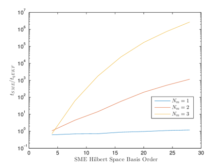
Refer to caption
(a) tSME/tqEKFsubscript𝑡𝑆𝑀𝐸subscript𝑡𝑞𝐸𝐾𝐹t_{SME}/t_{qEKF}
Refer to caption
(b) MISE comparison
Refer to caption
(c) q1subscript𝑞1q_{1} Error
Figure 1: (color online) Application of the quantum EKF to estimate quadratures of two cavity modes with Kerr Hamiltonians. Here, we use a cavity with damping constant γi=32subscript𝛾𝑖32\gamma_{i}=32 and Kerr nonlinearity constant χi=0.3πsubscript𝜒𝑖0.3𝜋\chi_{i}=0.3\pi. The Hilbert space basis for each modes is of order to 32. Figure 1a shows the ratio of one time-step computational time between the SME and the quantum EKF for various number of modes, and order of the Hilbert space basis used for solving the SME. The ratio increases dramatically when the number of modes increases. Figure 1b shows a comparison of the mean integral of squared quadratic error, 1T(0T𝐱~t,ω𝐱~t,ω𝑑t)1/21𝑇superscriptsuperscriptsubscript0𝑇superscriptsubscript~𝐱𝑡𝜔topsubscript~𝐱𝑡𝜔differential-d𝑡12\frac{1}{T}(\int_{0}^{T}\tilde{\mathbf{x}}_{t,\omega}^{\top}\tilde{\mathbf{x}}_{t,\omega}dt)^{1/2}, for the quantum EKF and SME estimation, with various different orders of the Hilbert space basis, against different initial coherent amplitudes α𝛼\alpha. The error 𝐱~t,ωsubscript~𝐱𝑡𝜔\tilde{\mathbf{x}}_{t,\omega} is approximated by subtracting the estimate of the quantum EKF and the SME against the estimate of the SME with the largest Hilbert space basis (32)32(32). Figure 1c shows the estimation of the first mode quadrature with different initial errors. The initial value of the quantum EKF is given by 𝐱^0,ω=𝐱^SME(0,ω)+ζ[111 1]subscript^𝐱0𝜔subscript^𝐱𝑆𝑀𝐸0𝜔𝜁superscriptdelimited-[]1111top\hat{\mathbf{x}}_{0,\omega}=\hat{\mathbf{x}}_{SME(0,\omega)}+\zeta[1\;-1\;-1\;1]^{\top}. ζ𝜁\zeta corresponds to the magnitude of the initial estimation error. In this simulation, the trajectories of the SME and the quantum EKF estimation are generated from identical measurement records.

In this example, we would like to estimate the quadratures of two cavity modes 𝐱i,t=[qipi],i=1,2formulae-sequencesubscript𝐱𝑖𝑡superscriptdelimited-[]subscript𝑞𝑖subscript𝑝𝑖top𝑖12\mathbf{x}_{i,t}=\left[q_{i}\;p_{i}\right]^{\top},i=1,2. Each mode has an identical Kerr Hamiltonian and a direct coupling Hamiltonian. For n𝑛n cavity modes, the direct coupling Hamiltonian is given by [52], int=i,j=1ijniγij(ajaiaiaj)=i=1j=i+1n𝐱i,t𝐒˘ij𝐱j,tsubscript𝑖𝑛𝑡superscriptsubscript𝑖𝑗1𝑖𝑗𝑛𝑖subscript𝛾𝑖𝑗subscript𝑎𝑗subscriptsuperscript𝑎𝑖subscript𝑎𝑖subscriptsuperscript𝑎𝑗superscriptsubscript𝑖1𝑗𝑖1𝑛superscriptsubscript𝐱𝑖𝑡topsubscript˘𝐒𝑖𝑗subscript𝐱𝑗𝑡\mathbb{H}_{int}=\sum\limits_{\begin{subarray}{c}i,j=1\\ i\neq j\end{subarray}}^{n}i\sqrt{\gamma_{ij}}\left(a_{j}a^{\dagger}_{i}-a_{i}a^{\dagger}_{j}\right)=\sum\limits_{\begin{subarray}{c}i=1\\ j=i+1\end{subarray}}^{n}\mathbf{x}_{i,t}^{\top}\breve{\mathbf{S}}_{ij}\mathbf{x}_{j,t}. The parameters for the optical cavity, are given by 𝕊=𝐈,𝕃i=γai=𝐂i𝐱i,tformulae-sequence𝕊𝐈subscript𝕃𝑖𝛾subscript𝑎𝑖superscriptsubscript𝐂𝑖topsubscript𝐱𝑖𝑡\mathbb{S}=\mathbf{I},\mathbb{L}_{i}=\sqrt{\gamma}a_{i}=\mathbf{C}_{i}^{\top}\mathbf{x}_{i,t}, and

=i=1nχiai2ai2+i=1j=i+1n𝐱i,t𝐒˘ij𝐱j,t.superscriptsubscript𝑖1𝑛subscript𝜒𝑖superscriptsuperscriptsubscript𝑎𝑖2superscriptsubscript𝑎𝑖2superscriptsubscript𝑖1𝑗𝑖1𝑛superscriptsubscript𝐱𝑖𝑡topsubscript˘𝐒𝑖𝑗subscript𝐱𝑗𝑡\mathbb{H}=\sum\limits_{i=1}^{n}\chi_{i}{a_{i}^{\dagger}}^{2}a_{i}^{2}+\sum\limits_{\begin{subarray}{c}i=1\\ j=i+1\end{subarray}}^{n}\mathbf{x}_{i,t}^{\top}\breve{\mathbf{S}}_{ij}\mathbf{x}_{j,t}.

Let 𝚺=[0110]𝚺matrix0missing-subexpression11missing-subexpression0\bm{\Sigma}=\begin{bmatrix}0&&1\\ -1&&0\end{bmatrix}. The quantum Markovian generator for 𝐱tsubscript𝐱𝑡\mathbf{x}_{t}, is given by 𝐟i(𝐱t)=j=0n𝐀ij𝐱j,t+𝐟i,Kerr(𝐱i,t)subscript𝐟𝑖subscript𝐱𝑡superscriptsubscript𝑗0𝑛subscript𝐀𝑖𝑗subscript𝐱𝑗𝑡subscript𝐟𝑖𝐾𝑒𝑟𝑟subscript𝐱𝑖𝑡\mathbf{f}_{i}(\mathbf{x}_{t})=\sum\limits_{j=0}^{n}\mathbf{A}_{ij}\mathbf{x}_{j,t}+\mathbf{f}_{i,Kerr}(\mathbf{x}_{i,t}), while 𝐆i=i𝚺𝐂isubscript𝐆𝑖𝑖𝚺subscript𝐂𝑖\mathbf{G}_{i}=i\bm{\Sigma}\mathbf{C}_{i}. Now 𝐀ijsubscript𝐀𝑖𝑗\mathbf{A}_{ij} is given by the following matrices

𝐀ij={𝚺(𝐂i𝐂i),i=j𝚺𝐒˘ij,ij.\mathbf{A}_{ij}=\begin{cases}-\bm{\Sigma}\Im\left(\mathbf{C}_{i}\mathbf{C}_{i}^{\dagger}\right)&,i=j\\ \bm{\Sigma}\breve{\mathbf{S}}_{ij}&,i\neq j\end{cases}.

𝐟i,Kerr(𝐱t)subscript𝐟𝑖𝐾𝑒𝑟𝑟subscript𝐱𝑡\mathbf{f}_{i,Kerr}(\mathbf{x}_{t}) is the nonlinearity from the Kerr Hamiltonian, we have {dgroup*}

𝐟i,Kerr=χ4[4pi,t3+pi,tqi,t2+qi,t2pi,t+2qi,tpi,tqi,t8pi,t(4qi,t3+qi,tpi,t2+pi,t2qi,t+2pi,tqi,tpi,t8qi,t)]subscript𝐟𝑖𝐾𝑒𝑟𝑟𝜒4matrix4superscriptsubscript𝑝𝑖𝑡3subscript𝑝𝑖𝑡superscriptsubscript𝑞𝑖𝑡2superscriptsubscript𝑞𝑖𝑡2subscript𝑝𝑖𝑡2subscript𝑞𝑖𝑡subscript𝑝𝑖𝑡subscript𝑞𝑖𝑡8subscript𝑝𝑖𝑡4superscriptsubscript𝑞𝑖𝑡3subscript𝑞𝑖𝑡superscriptsubscript𝑝𝑖𝑡2superscriptsubscript𝑝𝑖𝑡2subscript𝑞𝑖𝑡2subscript𝑝𝑖𝑡subscript𝑞𝑖𝑡subscript𝑝𝑖𝑡8subscript𝑞𝑖𝑡\mathbf{f}_{i,Kerr}=\frac{\chi}{4}\begin{bmatrix}4p_{i,t}^{3}+p_{i,t}q_{i,t}^{2}+q_{i,t}^{2}p_{i,t}+2q_{i,t}p_{i,t}q_{i,t}-8p_{i,t}\\ -\left(4q_{i,t}^{3}+q_{i,t}p_{i,t}^{2}+p_{i,t}^{2}q_{i,t}+2p_{i,t}q_{i,t}p_{i,t}-8q_{i,t}\right)\end{bmatrix}

,

𝐅i(𝐱)=χ[qi,tpi,t+pi,tqi,t3pi,t2+0.5(qi,t2+pi,t2)2(3qi,t2+0.5(qi,t2+pi,t2)2)(qi,tpi,t+pi,tqi,t)].subscript𝐅𝑖𝐱𝜒matrixsubscript𝑞𝑖𝑡subscript𝑝𝑖𝑡subscript𝑝𝑖𝑡subscript𝑞𝑖𝑡missing-subexpression3superscriptsubscript𝑝𝑖𝑡20.5superscriptsubscript𝑞𝑖𝑡2superscriptsubscript𝑝𝑖𝑡223superscriptsubscript𝑞𝑖𝑡20.5superscriptsubscript𝑞𝑖𝑡2superscriptsubscript𝑝𝑖𝑡22missing-subexpressionsubscript𝑞𝑖𝑡subscript𝑝𝑖𝑡subscript𝑝𝑖𝑡subscript𝑞𝑖𝑡\mathbf{F}_{i}\left(\mathbf{x}\right)=\chi\begin{bmatrix}q_{i,t}p_{i,t}+p_{i,t}q_{i,t}&&3p_{i,t}^{2}+0.5\left(q_{i,t}^{2}+p_{i,t}^{2}\right)-2\\ -(3q_{i,t}^{2}+0.5\left(q_{i,t}^{2}+p_{i,t}^{2}\right)-2)&&-(q_{i,t}p_{i,t}+p_{i,t}q_{i,t})\end{bmatrix}.

We consider homodyne detection on each cavity mode as measurement such that 𝐄=𝐈,𝐍=0formulae-sequence𝐄𝐈𝐍0\mathbf{E}=\mathbf{I},\mathbf{N}=0. From Figure 1c, it can be seen that under a small error at time zero, the quantum EKF still maintains the estimation error to be bounded, which shows the convergence of the quantum EKF.
We can observe from Figure 2 that the area of mean and one standard deviation of the quantum EKF on the q1subscript𝑞1q_{1},p1subscript𝑝1p_{1},q2subscript𝑞2q_{2} and p2subscript𝑝2p_{2} are quite narrow and contained in the estimation of SME. In contrast, the quantum KF estimation has a substantially larger deviation from the truncated SME mean although it has a narrower standard deviation range.
Regarding the computational time, with a Hilbert space basis of order 20 on each mode, the SME requires nearly 200 times that of the quantum EKF. The SME will require 170,000 times that of the quantum EKF if the number of modes equals to three, see also Figure 1a. From Section 3.2, generally for every single mode increase in the quantum systems, the required time of the SME single step computation will be increased to by a factor of Ns3superscriptsubscript𝑁𝑠3N_{s}^{3}.
In terms of estimation error, the quantum EKF can mantain a fairly low slope of the mean integral of squared quadratic error, 1T(0T𝐱~t,ω𝐱~t,ω𝑑t)1/21𝑇superscriptsuperscriptsubscript0𝑇superscriptsubscript~𝐱𝑡𝜔topsubscript~𝐱𝑡𝜔differential-d𝑡12\frac{1}{T}(\int_{0}^{T}\tilde{\mathbf{x}}_{t,\omega}^{\top}\tilde{\mathbf{x}}_{t,\omega}dt)^{1/2} regardless of the initial state of the estimated quantum system. This is another benefit, since for the SME, the MISE could make a huge difference if the initial state needs a higher order Hilbert space basis, see Figure 1b.
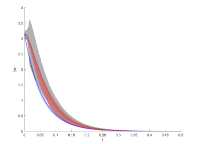
Refer to caption
(a) q1subscript𝑞1q_{1} averaged
Refer to caption
(b) p1subscript𝑝1p_{1} averaged
Refer to caption
(c) Phase space
Refer to caption
(d) q2subscript𝑞2q_{2} averaged
Refer to caption
(e) p2subscript𝑝2p_{2} averaged
Refer to caption
(f) Phase space
Figure 2: (color online) As in Figure 1, this simulation shows a comparison of the quantum EKF, the SME, and the quantum Kalman Filter (KF) estimation results. The black line with a shaded area corresponds to the mean with one standard deviation range from 100 Monte Carlo trials of the SME’s estimation (Hilbert space basis of order 20 for each mode). The red line with a shaded area is the quantum EKF and the blue line is the estimation of the quantum KF where we simply ignore the nonlinearity. Initial errors are set to zero for these simulations.

4.2 Estimating the quadratures of an optical cavity subject to simultaneous homodyne detection and photon counting

Refer to caption
Figure 3: Simultaneous photon counting and homodyne detection at either output port of a beam splitter in a quantum optics experiment, and the corresponding quantum network depiction of the quantum optics setup, [12].

Figure 3 shows an optical cavity with the simultaneous homodyne detection and photon counting setup as considered in [12]. The involvement of photon counting in this optical setup makes the covariance matrix of the measurement 𝐑𝐑\mathbf{R} state-dependent.
Let 𝒢1subscript𝒢1\mathcal{G}_{1} be our system of interest, with parameters (𝟙,γa,)1𝛾𝑎(\mathbb{1},\sqrt{\gamma}a,\mathbb{H}). The vacuum noise is concatenated into our system by 𝒢2subscript𝒢2\mathcal{G}_{2}, whose parameters are (𝟙,0,0)100(\mathbb{1},0,0). The beam splitter is given by 𝒢3subscript𝒢3\mathcal{G}_{3}, with parameters (𝕊,0,0)𝕊00(\mathbb{S},0,0). By taking the series and the concatenation products [39], the parameters of the composite quantum system in Figure 3 are given by 𝒢=(𝒢1𝒢2)𝒢3𝒢contains-as-subgroupsubscript𝒢1subscript𝒢2subscript𝒢3\mathcal{G}=\left(\mathcal{G}_{1}\boxplus\mathcal{G}_{2}\right)\rhd\mathcal{G}_{3}, with (𝕊,𝕊(γa0),)𝕊𝕊matrix𝛾𝑎0\left(\mathbb{S},\mathbb{S}\begin{pmatrix}\sqrt{\gamma}a\\ 0\end{pmatrix},\mathbb{H}\right).
The beam splitter matrix 𝕊𝕊\mathbb{S}, bath coupling 𝕃𝕃\mathbb{L} and Hamiltonian \mathbb{H} are given by the following {dgroup*}

𝕊=[1r2irir1r2],r0,𝕃=𝕊𝐂𝐱t,formulae-sequence𝕊matrix1superscript𝑟2𝑖𝑟𝑖𝑟1superscript𝑟2formulae-sequence𝑟0𝕃𝕊superscript𝐂topsubscript𝐱𝑡{\mathbb{S}=\begin{bmatrix}\sqrt{1-r^{2}}&ir\\ ir&\sqrt{1-r^{2}}\end{bmatrix},\;r\geq 0,\;\mathbb{L}=\mathbb{S}\mathbf{C}^{\top}\mathbf{x}_{t}},
=i(ηa2ηa2),η.formulae-sequence𝑖superscript𝜂superscript𝑎2𝜂superscriptsuperscript𝑎2𝜂\mathbb{H}=i\left(\eta^{\ast}a^{2}-\eta{a^{\dagger}}^{2}\right),{\eta\in\mathbb{C}}.

Figures 4c-4d show a sample of Monte Carlo simulation of the SME (black), and the extension of the quantum EKF developed in Section 3.4 (rqEKF) (blue). In this trial, the system’s density operator is a superposition between a coherent and a Fock state. It is clear from Figs. 4c-4d that rqEKF estimation gives a good approximation to the solution of the SME after a transient period. In the event of photon detection however, the rqEKF tends to have a slightly higher instantaneous jumps compared to the SME.
Figures 4a-4b shows how the rqEKF performs against the truncated SME in terms of the average estimate of 100 Monte Carlo trials and their one standard average region. We first observe that the area of mean and one stdev of the rqEKF for qtsubscript𝑞𝑡q_{t} and ptsubscript𝑝𝑡p_{t} gives a qualitatively good approximation after a small transient time similar to those of the SME.
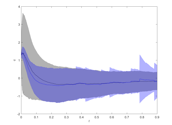
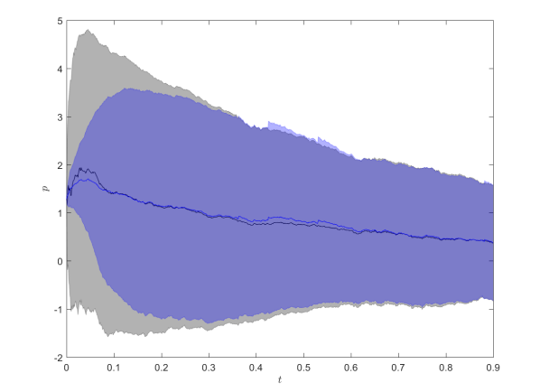
Refer to caption
(a) q𝑞q
Refer to caption
(b) p𝑝p
Refer to caption
(c) q𝑞q-trial
Refer to caption
(d) p𝑝p-trial
Figure 4: (color online) These figures show the estimation of the optical cavity quadratures subject to simultaneous homodyne detection and photon counting. The system’s Hilbert space basis (N) is of order 404040. The system’s initial vector state (unnormalized) is |ψ~0=0.5|n+0.5|αsubscriptket~𝜓00.5ket𝑛0.5ket𝛼\ket{\tilde{\psi}}_{0}=0.5\ket{n}+0.5\ket{\alpha}, with n=N/2,α=N/2exp(iπ/4)formulae-sequence𝑛𝑁2𝛼𝑁2𝑖𝜋4n=N/2,\alpha=\sqrt{N/2}\exp(i\pi/4), while the reflectivity factor r2superscript𝑟2r^{2} is 0.5. Figures 4a-4b show the mean and one standard deviation range of 100 Monte Carlo trajectories of the SME (black) and the robust quantum EKF. Figures 4c-4d, show q𝑞q and p𝑝p values from a sample of Monte Carlo trials.

5 Conclusion

In this article we have developed a quantum EKF for a class of nonlinear QSDEs describing an open quantum system subject to measurement. We derived a sufficient condition for the quantum EKF to achieve local quadratic exponential convergence in the estimation error. We also extended the quantum EKF to the class of quantum systems and measurements with state-dependent covariance matrices. Finally, we have illustrated via two examples the effectiveness of the quantum EKF approximation.

6 References

References

  • [1] Anderson B D O and Moore J B 1979 Optimal Filtering (Prentice-Hall)
  • [2] Belavkin V P 1980 Radiotechnika i Elektronika 25 1445–1453
  • [3] Wiseman H M and Milburn G J 2010 Quantum Measurement and Control (Cambridge University Press) ISBN 9780521804424
  • [4] Doherty A C and Jacobs K 1999 Phys. Rev. A: At., Mol., Opt. Phys. 60(4) 2700–2711
  • [5] Yamamoto N 2006 Phys. Rev. A: At., Mol., Opt. Phys. 74 032107
  • [6] Belavkin V P 1983 Automatica and Remote Control 44 178–188
  • [7] Belavkin V P 1989 Nondemolition measurements, nonlinear filtering and dynamic programming of quantum stochastic processes Modeling and Control of Systems (Lecture Notes in Control and Information Sciences vol 121) ed Blaquire A (Springer Berlin Heidelberg) pp 245–265 ISBN 978-3-540-50790-1
  • [8] Belavkin V P 1992 Comm. Math. Phys. 146 611–635
  • [9] Hume D B, Rosenband T and Wineland D J 2007 Phys. Rev. Lett. 99(12) 120502
  • [10] Sayrin C, Dotsenko I, Zhou X, Peaudecerf B, Rybarczyk T, Gleyzes S, Rouchon P, Mirrahimi M, Amini H, Brune M et al. 2011 Nature 477 73–77
  • [11] Wieczorek W, Hofer S G, Hoelscher-Obermaier J, Riedinger R, Hammerer K and Aspelmeyer M 2015 Phys. Rev. Lett. 114(22) 223601
  • [12] Emzir M F, Woolley M J and Petersen I R 2015 J. Phys. A-Math. Theor. 48 385302
  • [13] Doherty A C, Habib S, Jacobs K, Mabuchi H and Tan S M 2000 Phys. Rev. A 62
  • [14] Steck D A, Jacobs K, Mabuchi H, Habib S and Bhattacharya T 2006 Phys. Rev. A: At., Mol., Opt. Phys. 74(1) 012322
  • [15] Hush M R, Szigeti S S, Carvalho A R R and Hope J J 2013 New J. Phys. 15 113060
  • [16] Tsang M 2015 Phys. Rev. A 92
  • [17] Mathews V and Sicuranza G 2000 Polynomial signal processing Wiley series in telecommunications and signal processing (Wiley) ISBN 9780471034148
  • [18] Ljung L 1979 IEEE Trans. Automat. Contr. 24 36–50 ISSN 0018-9286
  • [19] Song Y and Grizzle J 1992 The extended kalman filter as a local asymptotic observer for nonlinear discrete-time systems Amer. Control Conf., 1992 pp 3365–3369
  • [20] La Scala B, Bitmead R and James M 1995 Math. Control Signal 8 1–26 ISSN 0932-4194
  • [21] Boutayeb M, Rafaralahy H and Darouach M 1997 IEEE Trans. Automat. Contr. 42 581–586 ISSN 0018-9286
  • [22] Reif K, Unbehauen R, Yaz E and Günther S 2000 IEE Proceedings - Control Theory and Applications 147 45–52
  • [23] Nazaikinskii V E, Shatalov V E and Sternin B Y 1996 Methods of Noncommutative Analysis (Walter de Gruyter GmbH)
  • [24] Birman M S and Solomyak M 2003 Integr. Equat. Oper. Th. 47 131–168
  • [25] Walls D F and Milburn G J 1994 Quantum Optics (Springer Science Business Media)
  • [26] Bouten L, Handel R V and James M R 2007 SIAM J. Contr. & Optim. 46 2199–2241
  • [27] Lipster R S and Shiryayev A N 2001 Statistics of Random Processes: I. General Theory Applications of mathematics : stochastic modelling and applied Probability (Springer) ISBN 9783540639299
  • [28] Lindblad G 1976 Comm. Math. Phys. 48 119–130
  • [29] Parthasarathy K R 1992 An Introduction to Quantum Stochastic Calculus Modern Birkhäuser classics (Springer)
  • [30] Sakai S 1971 C-algebras and W-algebras vol 60 (Springer Science & Business Media)
  • [31] Pedersen G K 2000 Publ. Res. Inst. Math. Sci. 36 139–157
  • [32] Widom H 1983 When are differentiable functions differentiable ? (Springer Verlag) chap 4 Operator Theory, pp 184–188 Lecture Notes in Mathematics
  • [33] Hutson V and Pym J 2005 Applications of Functional Analysis and Operator Theory Mathematics in Science and Engineering (Elsevier Science) ISBN 9780080527314
  • [34] Conway J B 2000 A course in operator theory vol 2 (American Mathematical Society)
  • [35] Farforovskaya Y B 1975 J. Math. Sci. 4 426–433
  • [36] Arazy J, Barton T and Friedman Y 1990 Integr. Equat. Oper. Th. 13 461–487
  • [37] Kissin E and Shulman V S 1996 Funct. Anal. Appl. 30 280–282
  • [38] Klebaner F C 2012 Introduction to Stochastic Calculus with Applications (World Scientific Pub Co Pte Lt)
  • [39] Gough J and James M 2009 IEEE Trans. Automat. Contr. 54 2530–2544
  • [40] Wiseman H M and Doherty A C 2005 Phys. Rev. Lett. 94(7) 070405
  • [41] Reif K, Sonnemann F and Unbehauen R 1998 Automatica 34 1119–1123
  • [42] Reif K, Sonnemann F and Unbehauen R 1999 IEEE Trans. Automat. Contr. 44 203–208
  • [43] Bernstein D 2009 Matrix Mathematics: Theory, Facts, and Formulas (Second Edition) Princeton reference (Princeton University Press) ISBN 9780691140391
  • [44] Sastry S 1999 Nonlinear systems: analysis, stability, and control vol 10 (Springer)
  • [45] Zakai M 1967 SIAM J. on Contr. 5 588–593
  • [46] Baras J S, Bensoussan A and James M R 1988 SIAM J. Appl. Math. 48 1147–1158
  • [47] Snyder D L 1972 IEEE Trans. Inform. Theory 18 91–102 ISSN 0018-9448
  • [48] Segall A and Kailath T 1975 IEEE Trans. Automat. Contr.
  • [49] Segall A, Davis M and Kailath T 1975 IEEE Trans. Inform. Theory 21 143–149
  • [50] Ceci C and Colaneri K 2012 Adv. in Appl. Probab. 44 678–701
  • [51] Ceci C and Colaneri K 2014 Appl. Math. Optim. 69 47–82
  • [52] Wiseman H M and Milburn G J 1994 Phys. Rev. A: At., Mol., Opt. Phys. 49(5) 4110–4125