Optimal sequence memory in driven random networks
Abstract
Autonomous randomly coupled neural networks display a transition to chaos at a critical coupling strength. We here investigate the effect of a time-varying input on the onset of chaos and the resulting consequences for information processing. Dynamic mean-field theory yields the statistics of the activity, the maximum Lyapunov exponent, and the memory capacity of the network. We find an exact condition that determines the transition from stable to chaotic dynamics and the sequential memory capacity in closed form. The input suppresses chaos by a dynamic mechanism, shifting the transition to significantly larger coupling strengths than predicted by local stability analysis. Beyond linear stability, a regime of coexistent locally expansive, but non-chaotic dynamics emerges that optimizes the capacity of the network to store sequential input.
∗ These authors contributed equally
pacs:
87.19.lj, 87.85.Ng, 05.45.-a, 05.40.-aLarge random networks of neuron-like units can exhibit collective chaotic dynamics (Sompolinsky et al., 1988; van Vreeswijk and Sompolinsky, 1996; Monteforte and Wolf, 2010; Lajoie et al., 2013). Their information processing capabilities have been a focus in neuroscience (Maass et al., 2002) and in machine learning (Jaeger and Haas, 2004) and show optimal performance close to the transition to chaos (Legenstein and Maass, 2007a; Sussillo and Abbott, 2009; Toyoizumi and Abbott, 2011). Due to its rich chaotic dynamics, the seminal network model by Sompolinsky et al. (Sompolinsky et al., 1988) until today serves as a model for various activity patterns observed in working memory tasks (Barak et al., 2013; Rajan et al., 2016; Li et al., 2016; Murray et al., 2016), motor control (Laje and Buonomano, 2013), and perceptual decision making (Mante et al., 2013). The interplay between a time-dependent input signal and the dynamical state of the network, however, is poorly understood; notwithstanding consequences for information processing.
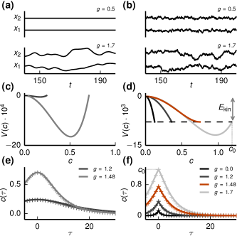
In the absence of a signal the network dynamics is autonomous. Networks of randomly coupled rate neurons display a transition from a fixed point to chaotic fluctuations at a critical coupling strength (Sompolinsky et al., 1988), illustrated in Figure 1a. The transition is well understood by dynamic mean-field theory, originally developed for spin glasses (Sompolinsky and Zippelius, 1981, 1982). The onset of chaos is equivalent to the emergence of a non-zero, decaying autocorrelation function, whose decay time diverges at the transition. This equivalence has been used in several subsequent studies (Rajan et al., 2010; Aljadeff et al., 2015; Harish and Hansel, 2015). Furthermore a tight relationship to random matrix theory exists: the transition happens precisely when the fixed point becomes linearly unstable, which identifies the spectral radius of the random connectivity matrix (Sommers et al., 1988; Rajan and Abbott, 2006) as the parameter controlling the transition.
These relations, however, lose their validity in the presence of fluctuating input: stochasticity per se decorrelates the network activity even if the dynamics is stable (Figure 1b), so that a decaying autocorrelation function does not necessarily indicate chaos. The stochastic drive, furthermore, causes perpetual fluctuations also in the regular regime. Therefore, a transition to chaos, if existent at all, must be of qualitatively different kind than the transition from the silent fixed point in the autonomous case. Time-dependent driving has indeed been found to stabilize network dynamics (Molgedey et al., 1992; Rajan et al., 2010). However, the mechanism is only understood for low-dimensional systems in the context of chaos synchronization by noise (Zhou and Kurths, 2002), in networks driven by deterministic signals (Rajan et al., 2010), and in systems with time-discrete dynamics (Molgedey et al., 1992). In the latter model, the effect of the fluctuating input on the transition to chaos is completely captured by its influence on the spectral radius of the Jacobian. Its single neuron dynamics, moreover, does not possess non-trivial temporal correlations. But these temporal correlations are indeed essential for the transition to chaos and for information processing in time-continuous systems, as we will show here.
Realistic continuous-time network models can generate complex but controlled responses to input (Sussillo and Abbott, 2009) that resemble activity patterns observed in motor cortex. In particular, the dynamical state of the network plays a crucial role during the involved learning process. However, the effect of the input on the dynamical state has remained obscure.
To investigate the generic influence of external input on the network state, we include additive white noise in the seminal model by Sompolinsky et al. (1988) and develop the dynamic mean-field theory for the resulting stochastic continuous-time dynamics. In contrast to the original work, we here reformulate the problem in terms of the functional formalism for stochastic differential equations (Martin et al., 1973; Janssen, 1976; De Dominicis, 1976; De Dominicis and Peliti, 1978; Schuecker et al., 2016). The application of the auxiliary field formulation known from large field theory (Moshe and Zinn-Justin, 2003) then allows us to derive the mean-field equations by a saddle point approximation. We find that the autocorrelation function is formally identical to the motion of a classical particle in a potential, where the noise amounts to an initial kinetic energy. We then determine the maximum Lyapunov exponent (Eckmann and Ruelle, 1985) by considering two copies of the system with different initial conditions (Derrida and Pomeau, 1986) in a replica calculation. Our main result is a closed-form condition for the transition from stable to chaotic dynamics. We find that the input suppresses chaos significantly more strongly than expected from time-local linear stability, the criterion valid in time-discrete systems. This observation is explained by a dynamic effect: the decrease of the maximum Lyapunov exponent is related to the sharpening of the autocorrelation function by the fluctuating drive. The regime in the phase diagram between local instability, as indicated by the spectral radius of the Jacobian, and transition to chaos, corresponding to a positive maximum Lypunov exponent, constitutes an as yet unreported dynamical regime that combines locally expansive dynamics with asymptotic stability. Moreover, in contrast to the autonomous case, the decay time of the autocorrelation function does not diverge at the transition. Its peak is strongly reduced by the input and occurs slightly above the critical coupling strength.
To study information processing capabilities we evaluate the capacity to reconstruct a past input signal by a linear readout of the present state, the so-called memory curve (Jaeger, 2001). Dynamic mean-field theory and a replica calculation lead to a closed form expression for the memory curve. We find that the memory capacity peaks within the expansive, non-chaotic regime, indicating that locally expansive while asymptotically stable dynamics is beneficial to store input sequences in the dynamics of the neural network.
I Dynamic Mean-field equation
We study the continuous-time dynamics of a random network of neurons, whose states evolve according to the system of stochastic differential equations
| (1) |
The are independent and identically Gaussian distributed random coupling weights with zero mean and variance , where the intensive gain parameter controls the recurrent coupling strength or, equivalently, the weight heterogeneity of the network. We further exclude self-coupling, setting . The time-varying inputs are pairwise independent Gaussian white-noise processes with autocorrelation function . We choose the sigmoidal transfer function , so that without input, for , the model agrees with the autonomous one studied in (Sompolinsky et al., 1988).
The dynamical system (1) contains two sources of randomness: the quenched disorder due to the random coupling weights and temporally fluctuating drive. A particular realization of the random couplings defines a fixed network configuration and its dynamical properties usually vary between different realizations. For large network size , however, certain quantities are self-averaging, meaning that their values for a typical realization can be obtained by an average over network configurations (Fischer and Hertz, 1991). An important example is the population-averaged autocorrelation function.
We here derive a dynamic mean-field theory that describes the statistical properties of the system under the joint distribution of disorder, noise, and possibly random initial conditions in the limit of large network size . The theory can be derived via a heuristic “local chaos” assumption (Amari, 1972) or using a generating functional formulation (Sompolinsky and Zippelius, 1982; Crisanti and Sompolinsky, 1987). We here follow the latter approach, because it casts the problem into the established language of statistical field theory for which a wealth of approximation techniques is available (Zinn-Justin, 1996). A mathematically rigorous proof uses large deviation techniques (Cabana and Touboul, 2013). The general idea is that for large network size the local recurrent input in (1) approaches a Gaussian process with self-consistently determined statistics.
We interpret the stochastic differential equations in the Ito-convention (Gardiner, 1985) and formulate the problem (1) in terms of a moment-generating functional . Using the Martin-Siggia-Rose-De Dominicis-Janssen path integral formalism (Martin et al., 1973; De Dominicis and Peliti, 1978; Altland and B., 2010) we obtain
| (2) | ||||
| (3) |
where denotes the scalar product in time and in neuron space and and represent a response field and a source field, respectively. The measures are defined as and with the subscript denoting the -th unit and the superscript denoting the -th time slice. The action in (3) contains all single unit properties, therefore excluding the coupling term , which is written explicitly in (2).
Assuming that the dynamics is self-averaging, we average over the quenched disorder in the connectivity and perform a saddle-point approximation (Appendix A). The resulting functional factorizes into terms
| (4) |
with denoting the average autocorrelation function of the non-linearly transformed activity of the units (33) and . The factorization reduces the network to non-interacting units, each on a background of an independent Gaussian noise with identical self-consistently determined statistics. At this level of approximation, the problem is hence equivalent to a single unit system. The effective equation of motion corresponding to this system can be read from (4) (Appendix A)
| (5) |
Here, is a Gaussian white-noise process as in (1), independent of . The centralized Gaussian process is fully specified by its autocorrelation function
| (6) |
II Effective equation of motion of the autocorrelation
Our goal is to determine the mean-field autocorrelation function , which, by self-averaging, also describes the population-averaged autocorrelation function. Assuming that is a stationary process, obeys the differential equation (Appendix B)
| (7) |
with . The Dirac- inhomogeneity originates from the white-noise autocorrelation function of the time-varying input and is absent in (Sompolinsky et al., 1988). The same inhomogeneity arises from Poisson spiking noise with (Kadmon and Sompolinsky, 2015), where is the population-averaged firing rate. In (7) we write , introducing the notation
| (8) | ||||
for an arbitrary function and the Gaussian integration measures . This representation holds since is itself a Gaussian process. Note that (8) reduces to a one-dimensional integral for and .
We formulate (7) as the one-dimensional motion of a classical particle in a potential:
| (9) |
where we define
| (10) |
with and following from Price’s theorem (Price, 1958; Papoulis, 1991). The autocorrelation here plays the role of the position of the particle and the time lag the role of time. The potential (10) depends on the initial value , which has to be determined self-consistently. We obtain from classical energy conservation . Considering and the symmetry of , the fluctuating drive in (9) amounts to an initial velocity and thus to the kinetic energy . Since , the solution and its first derivative must approach zero as . Thus we obtain the self-consistency condition for as
| (11) |
For the autonomous case, Figure 1c,e shows the resulting potential and the corresponding self-consistent autocorrelation function in the chaotic regime. Approaching the transition from above, the amplitude vanishes and the decay time of diverges (Sompolinsky et al., 1988). This picture breaks down in the driven case (Figure 1d,f), where is always nonzero, decays with finite time scale and has a kink at zero. The mean-field prediction is in excellent agreement with the population-averaged autocorrelation function obtained from numerical simulations of one network instance showing that the self-averaging property is fulfilled. In the following we derive a condition for the transition from stable to chaotic dynamics in the presence of the time-varying input.
III Effect of Input on the transition to chaos
The maximum Lyapunov exponent quantifies how sensitive the dynamics depends on the initial conditions (Eckmann and Ruelle, 1985). It measures the asymptotic growth rate of infinitesimal perturbations. For stochastic dynamics the stability of the solution for a fixed realization of the noise or equivalently the stochastic input is also characterized by the maximum Lyapunov exponent 111The theory of random dynamical systems makes this more precise; a brief overview is given in (Lajoie et al., 2013).: If it is negative, trajectories with different initial conditions converge to the same time-dependent solution; the dynamics is stable. If it is positive, the distance between two initially arbitrary close trajectories grows exponentially in time; the dynamics exhibits sensitive dependence on initial conditions and is hence chaotic.
We derive the maximum Lyapunov exponent by using dynamic mean-field theory. To this end, we consider two copies of the network distinguished by superscripts . These copies, or replicas, have identical coupling matrix and, for , are subject to the same realization of the stochastic input . The maximum Lyapunov exponent can be defined as the asymptotic growth rate of the Euclidean distance between trajectories of the two copies:
We now follow an idea by Derrida and Pomeau (1986) and exploit the self-averaging property of population-averaged correlation functions, i.e, , where denote the correlation functions averaged over the realization of the couplings. We express the mean squared Euclidean distance as
where we defined the mean-field squared distance . Thus the asymptotic growth rate of provides us with a mean-field description of the maximum Lyapunov exponent. To obtain this growth rate we first consider
| (12) |
with the obvious property . We then determine the temporal evolution of for infinitesimally perturbed initial conditions . To this end it is again convenient to use a generating functional that captures the joint statistics of the two systems and in addition allows averaging over the quenched disorder (see also Zinn-Justin, 1996, Appendix 23, last remark). The generating functional describing the two copies is defined analogously to the single system (2) as
| (13) |
with the single system “free action” defined in (3). The factor in the last line results from the identical external input in the two copies and effectively couples the two systems. We also note that the coupling matrix is the same in both copies.
Averaging (13) over the quenched disorder of the random coupling matrix and performing a saddle-point approximation we obtain a pair of effective dynamical equations (Appendix C),
| (14) |
together with a set of self-consistency equations for the statistics of the noises
| (15) |
Now, there are two terms which introduce correlations between the two copies. First the common temporal fluctuations injected into both systems. Second the effective noises and are correlated between replicas (15), arising from the two systems having the same coupling in each realization. The origin of the latter coupling is hence of static nature.
The distance (12) between the two copies is given by the auto-correlations of the single systems and the cross-correlations between them. We consider the case where both copies are prepared with identical initial conditions and thus are fully synchronized: the cross-correlation initially equals the auto-correlations , . The latter are identical to the single-system autocorrelation function , because the marginal statistics of each subsystem is not affected by the mere presence of the respective other system. An increase of the distance , by (12), amounts to a decline of away from its initial value . Here is the stationary autocorrelation as we are interested in the Lyapunov exponent averaged over initial conditions drawn from the stationary distribution. To determine the growth rate in the limit of small distances between the two copies we therefore expand the cross-correlation around its stationary solution , which leads to an equation of motion for the first order deflection (Appendix C.1)
| (16) |
with .
A separation ansatz in the coordinates and then yields an eigenvalue problem in the form of a time-independent Schr dinger equation (Sompolinsky et al., 1988; Kadmon and Sompolinsky, 2015) (Appendix C.2)
| (17) |
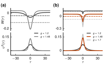
where now plays the role of a spatial coordinate. Here, the quantum potential is given by the negative second derivative of the classical potential evaluated along the self-consistent autocorrelation function . The ground state energy of (17) determines the asymptotic growth rate of as and, hence, the maximum Lyapunov exponent via (C.2). Therefore, the dynamics is predicted to become chaotic if . The quantum potential together with the solution for the ground state energy and wave function is shown in Figure 2. The latter are obtained as solutions of a finite difference discretization of (17).
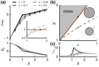
In the autonomous case, a decaying autocorrelation function corresponds to a positive maximum Lyapunov exponent (Sompolinsky et al., 1988). This follows from the observation that for the derivative of the self-consistent autocorrelation function solves the Schr dinger equation with . But as is an eigenfunction with a single node it cannot be the ground state, which has zero nodes. The ground state energy, which is necessarily lower, must therefore be negative, . So the dynamics is chaotic and crosses zero at (Figure 3a).
In the presence of fluctuating drive, the maximum Lyapunov exponent becomes positive at a critical coupling strength ; with increasing input amplitude the transition shifts to larger values (Figure 3a). The mean-field prediction shows excellent agreement with the maximum Lyapunov exponent obtained in simulations using a standard algorithm (Eckmann and Ruelle, 1985). Since the ground state energy must be larger than the minimum of the quantum potential, an upper bound for is provided by leading to a necessary condition
| (18) |
for chaotic dynamics. However, close to the transition is clearly smaller than the upper bound, which is a good approximation only for small (Figure 3a, inset): the actual transition occurs at substantially larger coupling strengths. In contrast, for memoryless discrete-time dynamics the necessary condition found here is also sufficient for the transition to chaos (Molgedey et al., 1992, eq. 13).
The local linear stability of the dynamical system (1) is analyzed via the variational equation
| (19) |
describing the temporal evolution of an infinitesimal deviation about a reference trajectory . Interestingly, (cf. (18)) is also the radius of the disk formed by the eigenvalues of the Jacobian matrix in the variational equation (19) estimated by random matrix theory (Sommers et al., 1988; Rajan and Abbott, 2006). Therefore, the dynamics is expected to become locally unstable if this radius exceeds unity, as shown in the inset in Figure 3b displaying and the eigenvalues at an arbitrary point in time. But even for the case with the system is not necessarily chaotic. Hence, contrary to the autonomous case (Sommers et al., 1988; Sompolinsky et al., 1988), the transition to chaos is not predicted by random matrix theory.
To derive an exact condition for the transition we determine a ground state with vanishing energy . As in the autonomous case, solves (17) for , except at where it exhibits a jump, because has a kink due to the input (7). By linearity is a continuous and symmetric solution with zero nodes. Therefore, if its derivative is continuous as well, requiring , it constitutes the searched for ground state. This is in contrast to the autonomous case, where corresponds to the first excited state. Consequently, with (7) we find the condition for the transition
| (20) |
in which is determined by the self-consistency condition (11) resulting in the transition curve in parameter space (Figure 3b). This reveals the relationship between the onset of chaos, the statistics of the random coupling matrix, and the input amplitude.
From (20) follows that the system becomes chaotic precisely when the variance of a typical single unit equals the variance of its recurrent input from the network . At the transition the classical self-consistent potential has a horizontal tangent at , while in the chaotic regime a minimum emerges (Figure 1d). This implies with (7) that the curvature of the autocorrelation function at zero changes sign from positive to negative (Figure 1f). Close to the transition a standard perturbative approach shows that is proportional to , indicating a self-stabilizing effect: since both terms grow with , the growth of their difference is attenuated, explaining why bends down as the transition is approached (Figure 3a).
The condition (20) predicts the transition at significantly larger coupling strengths compared to the necessary condition (Figure 3b), which is explained as follows. For continuous-time dynamics the effect of fluctuating input is twofold: First, because the slope is maximal at the origin, fluctuations reduce the averaged squared slope in , thereby stabilizing the dynamics. This is an essentially static effect as it can be fully attributed to the increase of the variance caused by the additional input; static heterogeneous inputs would have the same effect. Second, the input sharpens the autocorrelation function (Figure 1e,f) and hence the quantum potential (Figure 2). This shifts the ground-state energy to larger values, further decreasing the maximum Lyapunov exponent. Because this effect depends on the temporal correlations, the input suppresses chaos by a dynamic mechanism yielding stable dynamics even in the presence of local linear instability.
To understand this dynamic mechanism we return to the variational equation (19): its fundamental solution can be regarded as a product of short-time propagator matrices, where each factor has the same stability properties with unstable directions given by the local Jacobian matrix at the respective time. Even though the fraction of eigenvalues with positive real part stays approximately constant, the corresponding unstable directions vary in time. The sharpening of the autocorrelation function suggests that fluctuating input causes a faster variation, such that perturbations cannot grow in the direction of unstable modes, but rather decay asymptotically.
In low-dimensional systems the suppression of chaos by external fluctuations is understood: Noise forces the system to visit regions of the phase space with locally contracting dynamics more frequently (Zhou and Kurths, 2002) so that contraction dominates expansion, in total yielding stable asymptotic behavior. This mechanism is similar to the static stabilization effect described above, where fluctuating drive causes the system to sample regions of the phase space with smaller eigenvalues of the Jacobian. The self-averaging high-dimensional system, however, has a constant spectral radius over time and hence the dynamics is either locally contracting or locally expanding for all times. While the previous effects are explained by local stability, the dynamic suppression of chaos found here is a genuinely time-dependent mechanism, explained by the time evolution of the Jacobian.
In the autonomous case the time-scale of fluctuations diverges at the transition to chaos (Sompolinsky et al., 1988). We here consider the effect of the input on the asymptotic decay time of the autocorrelation function (Figure 3c). For weak input amplitude, the decay time peaks at the transition, corresponding to the diverging time scale in the autonomous case. For larger input amplitudes, the peak is strongly reduced and the maximum decay time is attained above the transition.
IV Information processing capabilities
We expect the expansive, non-chaotic regime to be beneficial for information processing: The local instability of the network ensures sufficient initial amplification of the impinging external signal. The asymptotic stability is required for the driving signal not to be corrupted by the unbounded amplification of small variations of the input; it is hence necessary to ensure generalization. In the following we investigate these ideas quantitatively by considering the sequential memory capacity of the network.
We focus on the component of the input that is received by all neurons with equal strength. In other words, the total input to each neuron is decomposed into the signal and the remaining inputs which act as noise. We then consider the dynamical short-term memory defined as the capacity to reconstruct the input from the state at time using a linear readout, , where is the number of readout neurons. The reconstruction capacity as a function of the delay time yields the memory curve (Jaeger, 2001), where is the minimal relative mean-squared error between readout and signal. Alternatively this measure quantifies the fidelity by which a sequence of past inputs can be reconstructed from the current network activity.
For optimal readout weights that minimize , the memory curve is given by (Jaeger, 2001; Dambre et al., 2012)
We follow the approach by Toyoizumi and Abbott (2011) and neglect the off-diagonal terms in , which is justifiable for a sparse readout with . Additionally, for large the diagonal terms are given by their mean-field value , identical for all units. Determining the memory curve (LABEL:eq:memory_def) then amounts to computing the sum of squared correlation functions between the signal and the network activity, which we obtain by a replica calculation (Appendix D). The key idea is to express the correlation functions as a sum of response functions ; this is possible due to the Gaussian statistics of . The calculation is similar to the derivation of the Schr dinger equation (Appendix C) with the difference, however, that the two replicas receive independent realizations of the inputs. The memory curve follows from a differential equation for the correlation between the two systems and is measured in units of the readout ratio (69):
| (22) |
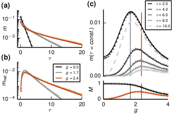
with the modified Bessel function of the first kind . The memory curve has two contributions (69): memory due to the collective network dynamics and local memory due to the leaky integration of the single units. The latter effect is trivial and is reflected in the initial steep falloff of the memory curves with time lag , independent of the coupling strength (Figure 4a). Its decay time is half the time constant of the neurons, which is set to unity here (1). With increasing coupling strength the variance increases, so that the memory curve (22) at zero time lag reduces. For time lags that are large compared to the single unit time constant, the network contribution to the memory dominates. A non-vanishing memory capacity for longer time lags is therefore only the result of the reverberation of the input through the network interaction. The analytical results are in excellent agreement with direct simulations.
We isolate the interesting network memory by subtracting the single unit contribution (first term in (69))
| (23) |
This quantity is particularly important in situations where the readout does not have access to the neurons receiving the signal. The network memory curve consistently vanishes for the uncoupled case. We compare the performance of two different couplings strengths: , following from (18) with equal sign and corresponding to the onset of the local instability, and , marking the onset of chaos (cf. Figure 3b). For short time lags, , the network memory curve is larger for , while for longer time lags it is larger for due to a slower decay of the memory curve. This behavior is confirmed by the memory curve as a function of , shown for different time lags (Figure 4c, upper panel). For , the memory capacity is entirely given by , which is in line with the fast decay of the single-unit contribution. Moreover, while for small time lags the memory is maximal around , for larger time lags it peaks nearby indicating that the intermediate, expansive, non-chaotic regime supports storage of the input.
The memory capacity is defined as the integral over the memory curve
| (24) |
which follows directly from the Laplace transform of the Bessel function.
Typically the memory capacity is bounded by the number of neurons (Dambre et al., 2012). The signal in our situation, however, can be seen as one out of independent inputs and its corresponding memory curve. The expressions are therefore independent of (Hermans and Schrauwen, 2010) and the memory capacity satisfies . The network memory capacity is defined as . While the memory capacity decreases in the chaotic regime, the network memory peaks within the expansive, non-chaotic regime (Figure 4b, lower panel).
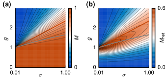
So far we have considered the memory capacity at a fixed amplitude of the input. In the following we investigate the memory capacity over the whole phase diagram. The total memory capacity shows a steep falloff directly above the onset of chaos (Figure 5a). This is expected because the information about the input is lost in the chaotic network dynamics. The contour lines of the memory capacity are nearly parallel to the transition criterion, the curve with vanishing Lyapunov exponent. This observation closely links the transition to chaos to the memory capacity: The direction in the phase diagram in which the system most quickly enters the chaotic regime is accompanied by the steepest decline of memory. The contour lines of the total network memory capacity show a ridge running through the expansive, non-chaotic regime (Figure 5b); it confirms the results found above: The memory is optimal in the dynamical regime of local instability and asymptotic stability. Moreover, the network capacity has a substantial contribution to the total memory capacity of about .
The optimal network memory in the hitherto unreported regime between and can be understood in an intuitive manner. Two conditions must be met for good memory. First, individual units must be susceptible to the signal; the susceptibility equals the noise-averaged slope of the gain function. Second, the signal must propagate effectively through the network, requiring a sufficiently strong coupling . These two requirements are reflected in the monotonic increase of the memory curve (22) with the effective slope , independent of the time lag . An increase in the coupling strength, however, elevates the intrinsically generated fluctuations as well. These have a twofold effect on the memory capacity. First they decrease , so that assumes a maximum. Second, the intrinsic fluctuations propagate through the network as well; they hence reduce the signal to noise ratio of the readout, as they enter the denominator in through . The interplay of these two mechanisms leads to optimal memory located in the expansive, non-chaotic regime, explaining why the combination of time-local expansive dynamics and stable long-term behavior maximizes the memory capacity of the network.
V Discussion
We here present a completely solvable network model that allows us to investigate the effect of time-varying input on the transition to chaos and information processing capabilities. Adding time-varying stochastic forcing to the seminal model by Sompolinsky et al. (1988) yields a stochastic continuous-time dynamical system. Contrary to the original model (Sompolinsky et al., 1988), we here reformulate the stochastic differential equations as a field theory (Martin et al., 1973; De Dominicis, 1976; Janssen, 1976; De Dominicis and Peliti, 1978). This formal step allows us to develop the dynamic mean-field theory by standard tools: a saddle point approximation of the auxiliary field generating functional (Sompolinsky and Zippelius, 1982; Crisanti and Sompolinsky, 1987; Moshe and Zinn-Justin, 2003). As in the original model, this procedure reduces the interacting system to the dynamics of a single unit. The self-consistent solution of the effective equation yields a standard physics problem: the autocorrelation function of a typical unit is given by the motion of a classical particle in a potential. We find that the amplitude of the input corresponds to the initial kinetic energy of the particle.
The field theoretical formulation then allows us to perform a replica calculation to determine the maximum Lyapunov exponent; the problem formally reduces to finding the ground-state energy of a single-particle quantum mechanical problem. The transition to chaos appears at the point where the ground state energy changes sign, which allows us to obtain a closed form condition relating the coupling strength and the input amplitude at the transition. We find a simple hallmark of the transition in the single unit activity: at the transition point the variance of the recurrent input to a single unit equals the variance of its own activity. Correspondingly, the autocorrelation function at zero time lag changes its curvature from convex to concave at the transition point. These features can readily be measured in most physical systems. The assessment of chaos by these passive observations in particular does not require a perturbation of the system.
The transition criterion allows us to map out the phase diagram spanned by the coupling strength and the input amplitude. It shows that external drive shifts the transition to chaos to significantly larger coupling strengths than predicted by time-local linear stability analysis. The transition in the stochastic system is thus qualitatively different from the transition in the autonomous system, where loss of local stability and transition to chaos are equivalent (Sompolinsky et al., 1988; Sommers et al., 1988). The discrepancy of these two measures in the driven system is explained by a dynamic effect: the decrease of the maximum Lyapunov exponent is related to the sharpening of the autocorrelation function by the fluctuating drive. The displacement between local instability and transition to chaos leads to an intermediate regime which is absent in time-discrete networks (Molgedey et al., 1992) and only exists in their more realistic time-continuous counterparts studied here. This hitherto unreported dynamical regime combines locally expansive dynamics with asymptotic stability.
The seminal works (Sompolinsky et al., 1988; Sommers et al., 1988) have established a tight link between the fields of random matrix theory and autonomous neural networks with random topology: Deterministic chaos emerges if the spectral radius of the coupling matrix exceeds unity. In contrast, we find in stochastically driven networks that the spectral radius only yields a necessary condition for a positive Lyapunov exponent; it determines the minimum of the quantum mechanical potential whose ground state energy relates to the Lyapunov exponent. The presented closed-form relation between input strength, the statistics of the random matrix, and the onset of chaos (20) generalizes the well known link to non-autonomous stochastic dynamics.
It is controversially discussed whether the instability of deterministic rate dynamics explains a transition to chaos in networks of spiking neurons (Ostojic, 2014; Engelken et al., 2015; Ostojic, 2015). It was argued that such a transition is absent in spiking models because the correlation time does not peak at the point where the corresponding deterministic rate dynamics becomes unstable (Engelken et al., 2015; Ostojic, 2015; Mastroguiseppe and Ostojic, 2016). For the analysis of oscillations (Brunel and Hakim, 1999) and correlations (Trousdale et al., 2012; Helias et al., 2013) in these networks, the irregular spiking activity of the neurons can be approximated by effective stochastic rate equations, whereby the realization of the spikes is represented by an explicit source of noise. In this setting, the input in (1) can be interpreted as such spiking noise, explicitly investigated in (Kadmon and Sompolinsky, 2015). For weak noise one may neglect its impact on the location of the transition. In this limit, noise suppresses the divergence of the correlation time (Kadmon and Sompolinsky, 2015). Our work is not bound to small noise amplitudes and suggests that a diverging time scale in spiking networks does not occur at the instability for two reasons. First, we have shown that in a stochastic system the transition to chaos is not predicted by local instability. If a diverging time-scale at the transition existed it would not occur at the instability, but as a larger coupling strength. But the presented analysis shows that the decay time of the autocorrelation function does not even peak at the transition to chaos, but rather in the chaotic regime. While these results strictly only hold for the rate dynamics considered here, they still strongly suggest the absence of a diverging time scale in networks of spiking neurons. Indeed, the absence of a diverging time-scale has been observed in simulation of spiking neurons (Engelken et al., 2015) as well as in an iterative approach solving for the self-consistent autocorrelation function (Dummer et al., 2014; Wieland et al., 2015).
To assess whether this richer dynamics found in the driven network has functional consequences, we investigate sequential memory (Jaeger, 2001). The obtained closed-form expression for the network memory capacity exhibits a peak within the expansive, non-chaotic regime. We identify two mechanisms whose partly antagonistic interplay causes optimal memory: Local amplification of the stimulus and intrinsically-generated noise. Local instability of the network ensures sensitivity to the external input, so that on short time scales the incoming signal is amplified and can therefore more reliably be read out. But larger coupling also increases network-intrinsic fluctuations, which, in turn, reduce the susceptibility as well as the signal to noise ratio of the readout. Therefore it is plausible that the optimal memory appears at a point where local amplification of the external input is large enough, but intrinsic chaoticity is still limited.
Sequential memory has been studied in a time-discrete neural network model (Toyoizumi and Abbott, 2011), which receives a single weak external input. In contrast, we here investigate the memory of a single signal in the presence of multiple simultaneous inputs with arbitrary amplitude . Without additional observation noise, Toyoizumi and Abbott (2011) find that sequential memory does not posses a maximum; it is constant and optimal for sub-critical coupling values and falls off in the chaotic regime due to intrinsically-generated fluctuations. Perfect reconstruction in the non-chaotic regime is possible, because the single-step delayed activity is a direct linear function of the input. In our setting, the single neuron memory has a similar effect (Figure 5 a). In the discrete system, optimal memory close to the transition only arises in presence of observation noise (Toyoizumi and Abbott, 2011). Memory falloff in the chaotic phase is much more shallow than in the direction of regular dynamics, so that a fine-tuning is not needed if the network dynamic is slightly chaotic.
For continuous dynamics the situation is qualitatively different. The network component of the memory or, equivalently, the memory for longer delay times , shows non-monotonic behavior even without observation noise. For small signal amplitude , memory is optimal right below the transition to chaos and steeply falls off above (Figure 5 b). For large , the falloff is weaker in the chaotic regime, qualitatively more similar to Toyoizumi and Abbott (2011).
A negative maximum Lyapunov exponent for nonautonomous dynamics indicates the echo state property, the reliability of the network response to input (Wainrib and Galtier, 2016). We could indeed show for the analytically tractable model here that memory capacity quickly declines in the chaotic regime due to intrinsically generated chaotic fluctuations. Echo state networks show long temporal memory near the edge of chaos (Bertschinger and Natschläger, 2004; Legenstein and Maass, 2007b; Büsing et al., 2010; Boedecker et al., 2012). Typically these networks are time-discrete and thus the onset of chaos is directly linked to the spectral radius of the Jacobian. This relation is used in the design of these systems, exploiting that a spectral radius close to local instability ensures long memory times. We here show for the driven and time-continuous system, that the edge of chaos and local instability are two different concepts and that memory capacity is a third, distinct measure: Memory is optimal at neither of the two other criteria, but rather in between. In particular, our analytical results for the memory capacity can be used to determine the optimal coupling strength for a given input amplitude.
Recently, an algorithm was proposed to train a random network as given by (1) to produce a wide range of activity patterns (Sussillo and Abbott, 2009). Such learning shows best performance if initially the random network without input is in the chaotic state. It has been argued that such networks have a large dynamic range and are able to produce a wide variety of outputs. In the training phase the input to the network needs to suppress chaos so that learning converges. The procedure therefore requires the choice of an initial coupling that is large enough to ensure chaos, but not too large so that the input can suppress chaos. Our quantitative criterion for the transition easily enables a proper choice of parameters and facilitates the design, control, and understanding of functional networks.
In this work we have considered memory of the input signal. An important task of the brain, however, is not only to maintain the input but also to perform non-linear transformations on it. We expect the locally unstable but globally stable dynamics to be beneficial for such a task: The expansive behavior can project the input into a high-dimensional space, which is crucial for non-linear computations or discrimination tasks (Legenstein and Maass, 2007b). Thus, this dynamical regime not only provides memory but might serve as a basis for more complex computations.
To show the generic effect of input we added a time-varying input to the seminal model by Sompolinsky et al. (1988). Even though the original model makes some simplifying assumptions, such as the all-to-all Gaussian connectivity and a sigmoidal symmetric gain function, the transition to chaos is qualitatively the same as in networks with more biologically realistic parameters (Mastroguiseppe and Ostojic, 2016; Kadmon and Sompolinsky, 2015; Harish and Hansel, 2015). To focus on the new physics arising in non-autonomous systems, we have here chosen to present the simplest but non-trivial, and yet application-relevant extension. The reformulation of the derivation of the dynamic mean-field theory by help of established methods from field theory (Sompolinsky and Zippelius, 1982; Crisanti and Sompolinsky, 1987; Moshe and Zinn-Justin, 2003; Chow and Buice, 2015; Hertz et al., 2017) here allowed us to find the explicit form of network memory by a replica calculation. In general, the presented formulation opens the study of recurrent random networks to the rich and powerful set of field theoretical methods developed in other branches of physics. This language allows a straight-forward extension of our results in various directions. Among them more biologically realistic settings, such as sparse connectivity respecting Dale’s law (Eccles et al., 1954), threshold like-activation functions, non-negative activity variables or multiple populations. The latter extension would allow the study of the interesting case in which the population receiving the signal is separated from the readout population. Such a situation would most likely emerge in the cortex where the input population of local microcircuits typically differs from the output population.
More generally, the stability of complex dynamical systems plays an important role in various other field of physics, biology, and technology. Examples include oscillator networks (Rodrigues et al., 2016), disordered soft-spin models (Sompolinsky and Zippelius, 1981), power grids (Nishikawa and Motter, 2015), food webs (Allesina and Tang, 2015), and gene-regularity networks (Pomerance et al., 2009). Presenting exact results for a prototypical and solvable model this work contributes to the understanding of chaos and signal propagation in such high dimensional systems.
VI Acknowledgements
This work was partially supported by Helmholtz young investigator’s group VH-NG-1028, Helmholtz portfolio theme SMHB, J lich Aachen Research Alliance (JARA). This project received funding from the European Union’s Horizon 2020 research and innovation programme under grant agreement No. 720270. J.S. and S.G. contributed equally to this work.
References
- Sompolinsky et al. (1988) H. Sompolinsky, A. Crisanti, and H. J. Sommers, Phys. Rev. Lett. 61, 259 (1988).
- van Vreeswijk and Sompolinsky (1996) C. van Vreeswijk and H. Sompolinsky, Science 274, 1724 (1996).
- Monteforte and Wolf (2010) M. Monteforte and F. Wolf, Phys. Rev. Lett. 105, 268104 (2010).
- Lajoie et al. (2013) G. Lajoie, K. K. Lin, and E. Shea-Brown, Phys. Rev. E 87, 052901 (2013).
- Maass et al. (2002) W. Maass, T. Natschläger, and H. Markram, Neural Comput. 14, 2531 (2002).
- Jaeger and Haas (2004) H. Jaeger and H. Haas, Science 304, 78 (2004).
- Legenstein and Maass (2007a) R. Legenstein and W. Maass, Neural Networks 20, 323 (2007a).
- Sussillo and Abbott (2009) D. Sussillo and L. F. Abbott, Neuron 63, 544 (2009).
- Toyoizumi and Abbott (2011) T. Toyoizumi and L. F. Abbott, Phys. Rev. E 84, 051908 (2011).
- Barak et al. (2013) O. Barak, D. Sussillo, R. Romo, M. Tsodyks, and L. Abbott, 103, 214 (2013).
- Rajan et al. (2016) K. Rajan, C. D. Harvey, and D. W. Tank, Neuron 90, 128 (2016).
- Li et al. (2016) N. Li, K. Daie, K. Svoboda, and S. Druckmann, Nature 532, 459 (2016).
- Murray et al. (2016) J. D. Murray, A. Bernacchia, N. A. Roy, C. Constantinidis, R. Romo, and X.-J. Wang, Proc. Nat. Acad. Sci. USA p. 201619449 (2016).
- Laje and Buonomano (2013) R. Laje and D. V. Buonomano, Nat. Neurosci. 16, 925 (2013).
- Mante et al. (2013) V. Mante, D. Sussillo, K. V. Shenoy, and W. T. Newsome, Nature 503, 78 (2013).
- Sompolinsky and Zippelius (1981) H. Sompolinsky and A. Zippelius, Phys. Rev. Lett. 47, 359 (1981).
- Sompolinsky and Zippelius (1982) H. Sompolinsky and A. Zippelius, Phys. Rev. B 25, 6860 (1982).
- Rajan et al. (2010) K. Rajan, L. Abbott, and H. Sompolinsky, Phys. Rev. E 82, 011903 (2010).
- Aljadeff et al. (2015) J. Aljadeff, M. Stern, and T. Sharpee, Phys. Rev. Lett. 114, 088101 (2015).
- Harish and Hansel (2015) O. Harish and D. Hansel, PLoS Comput Biol 11, e1004266 (2015).
- Sommers et al. (1988) H. Sommers, A. Crisanti, H. Sompolinsky, and Y. Stein, Phys. Rev. Lett. 60, 1895 (1988).
- Rajan and Abbott (2006) K. Rajan and L. F. Abbott, Phys. Rev. Lett. 97, 188104 (2006).
- Molgedey et al. (1992) L. Molgedey, J. Schuchhardt, and H. Schuster, Phys. Rev. Lett. 69, 3717 (1992).
- Zhou and Kurths (2002) C. Zhou and J. Kurths, Phys. Rev. Lett. 88, 230602 (2002).
- Martin et al. (1973) P. Martin, E. Siggia, and H. Rose, Phys. Rev. A 8, 423 (1973).
- Janssen (1976) H.-K. Janssen, Zeitschrift für Physik B Condensed Matter 23, 377 (1976).
- De Dominicis (1976) C. De Dominicis, J. Phys. Colloques 37, C1 (1976).
- De Dominicis and Peliti (1978) C. De Dominicis and L. Peliti, Phys. Rev. B 18, 353 (1978).
- Schuecker et al. (2016) J. Schuecker, S. Goedeke, D. Dahmen, and M. Helias, arXiv (2016), 1605.06758 [cond-mat.dis-nn].
- Moshe and Zinn-Justin (2003) M. Moshe and J. Zinn-Justin, Physics Reports 385, 69 (2003), ISSN 0370-1573.
- Eckmann and Ruelle (1985) J.-P. Eckmann and D. Ruelle, Reviews of modern physics 57, 617 (1985).
- Derrida and Pomeau (1986) B. Derrida and Y. Pomeau, EPL (Europhysics Letters) 1, 45 (1986).
- Jaeger (2001) H. Jaeger, Short term memory in echo state networks, vol. 5 (GMD-Forschungszentrum Informationstechnik, 2001).
- Fischer and Hertz (1991) K. Fischer and J. Hertz, Spin glasses (Cambridge University Press, 1991).
- Amari (1972) S.-I. Amari, Systems, Man and Cybernetics, IEEE Transactions on pp. 643–657 (1972).
- Crisanti and Sompolinsky (1987) A. Crisanti and H. Sompolinsky, Phys. Rev. A 36, 4922 (1987).
- Zinn-Justin (1996) J. Zinn-Justin, Quantum field theory and critical phenomena (Clarendon Press, Oxford, 1996).
- Cabana and Touboul (2013) T. Cabana and J. Touboul, J. statist. Phys. 153, 211 (2013).
- Gardiner (1985) C. W. Gardiner, Handbook of Stochastic Methods for Physics, Chemistry and the Natural Sciences (Springer-Verlag, Berlin, 1985), 2nd ed., ISBN 3-540-61634-9, 3-540-15607-0.
- Altland and B. (2010) A. Altland and S. B., Concepts of Theoretical Solid State Physics (Cambridge university press, 2010).
- Kadmon and Sompolinsky (2015) J. Kadmon and H. Sompolinsky, Phys. Rev. X 5, 041030 (2015).
- Price (1958) R. Price, IRE Transactions on Information Theory 4, 69 (1958).
- Papoulis (1991) A. Papoulis, Probability, Random Variables, and Stochastic Processes (McGraw-Hill, Boston, Massachusetts, 1991), 3rd ed.
- Note (1) Note1, the theory of random dynamical systems makes this more precise; a brief overview is given in (Lajoie et al., 2013).
- Dambre et al. (2012) J. Dambre, D. Verstraeten, B. Schrauwen, and S. Massar, Scientific reports 2, 514 (2012).
- Hermans and Schrauwen (2010) M. Hermans and B. Schrauwen, in Neural Networks (IJCNN), The 2010 International Joint Conference on (IEEE, 2010), pp. 1–7.
- Ostojic (2014) S. Ostojic, Nat. Neurosci. 17, 594 (2014).
- Engelken et al. (2015) R. Engelken, F. Farkhooi, D. Hansel, C. van Vreeswijk, and F. Wolf, bioRxiv p. 017798 (2015).
- Ostojic (2015) S. Ostojic, bioRxiv p. 020354 (2015).
- Mastroguiseppe and Ostojic (2016) F. Mastroguiseppe and S. Ostojic, arXiv p. 1605.04221 (2016).
- Brunel and Hakim (1999) N. Brunel and V. Hakim, Neural Comput. 11, 1621 (1999).
- Trousdale et al. (2012) J. Trousdale, Y. Hu, E. Shea-Brown, and K. Josic, PLOS Comput. Biol. 8, e1002408 (2012).
- Helias et al. (2013) M. Helias, T. Tetzlaff, and M. Diesmann, New J. Phys. 15, 023002 (2013).
- Dummer et al. (2014) B. Dummer, S. Wieland, and B. Lindner, Front. Comput. Neurosci. 8, 104 (2014).
- Wieland et al. (2015) S. Wieland, D. Bernardi, T. Schwalger, and B. Lindner, Phys. Rev. E 92, 040901 (2015).
- Wainrib and Galtier (2016) G. Wainrib and M. N. Galtier, Neural Networks 76, 39 (2016), ISSN 0893-6080.
- Bertschinger and Natschläger (2004) N. Bertschinger and T. Natschläger, Neural Comput. 16, 1413 (2004).
- Legenstein and Maass (2007b) R. Legenstein and W. Maass, What makes a dynamical system computationally powerful? (MIT Press, 2007b), pp. 127–154.
- Büsing et al. (2010) L. Büsing, B. Schrauwen, and R. Legenstein, Neural Comput. 22, 1272 (2010).
- Boedecker et al. (2012) J. Boedecker, O. Obst, J. T. Lizier, N. M. Mayer, and M. Asada, Theory in Biosciences 131, 205 (2012).
- Chow and Buice (2015) C. Chow and M. Buice, The Journal of Mathematical Neuroscience 5 (2015).
- Hertz et al. (2017) J. A. Hertz, Y. Roudi, and P. Sollich, Journal of Physics A: Mathematical and Theoretical 50, 033001 (2017).
- Eccles et al. (1954) J. Eccles, F. P, and K. Koketsu, J Physiol (Lond) 126, 524 (1954).
- Rodrigues et al. (2016) F. A. Rodrigues, T. K. D. Peron, P. Ji, and J. Kurths, Phys. Rep. 610, 1 (2016).
- Nishikawa and Motter (2015) T. Nishikawa and A. E. Motter, New J. Phys. 17, 015012 (2015).
- Allesina and Tang (2015) S. Allesina and S. Tang, Population Ecology 57, 63 (2015).
- Pomerance et al. (2009) A. Pomerance, E. Ott, M. Girvan, and W. Losert, Proc. Nat. Acad. Sci. USA 106, 8209 (2009).
- Negele and Orland (1998) J. W. Negele and H. Orland, Quantum Many-Particle Systems (Perseus Books, 1998).
- Abramowitz and Stegun (1974) M. Abramowitz and I. A. Stegun, Handbook of Mathematical Functions: with Formulas, Graphs, and Mathematical Tables (Dover Publications, New York, 1974).
Appendix A Derivation of mean-field equation
The generating functional in (2) is properly normalized independent of the realization of . This property allows us to follow (De Dominicis and Peliti, 1978) and to introduce the disorder-averaged generating functional
| (25) | ||||
The coupling term in (2) factorizes over unit indices and the random weights appear linear in the exponent. Thus we can separately integrate over the independently and identically distributed by completing the square and obtain
We reorganize the resulting sum in the exponent of the coupling term as
| (27) | |||||
where we used in the first step and in the second. The last line is the diagonal (self-coupling) to be skipped in the double sum. It is a correction of order and will be neglected in the following. The disorder-averaged generating functional (25) therefore takes the form
| (28) | |||||
where we extended our notation with to bi-linear forms and defined
| (29) |
The field is an empirical average over contributions, which, by the law of large numbers and in the case of weak correlations, will converge to its expectation value for large . This heuristic argument is shown in the following more formally: A saddle-point approximation leads to the replacement of by its (self-consistent) expectation value. To this end we first decouple the interaction term by inserting the Fourier representation of the Dirac- functional:
| (30) | ||||
where we further extended our notation with and . We note that the conjugate field is purely imaginary. We hence rewrite (28) as
| (31) | ||||
where we introduced source terms for the auxiliary fields and dropped the original source terms . The integral measures must be defined suitably. In writing we have used that the auxiliary fields couple only to sums of fields and , so that the generating functional for the fields and factorizes into a product of identical factors .
The remaining problem can be considered a field theory for the auxiliary fields and . The form (31) clearly exposes the dependence of the action for these latter fields: It is of the form , which, for large , suggests a saddle point approximation, which neglects fluctuations in the auxiliary fields and hence sets them equal to their expectation value; this point is the dominant contribution to the probability mass. To obtain the saddle point equations we consider the Legendre-Fenchel transform of as
called the vertex generating functional or effective action (Zinn-Justin, 1996; Negele and Orland, 1998). It holds that and , called equations of state. The leading order mean-field or tree-level approximation amounts to the approximation , where is the action for the auxiliary fields and . We insert this tree-level approximation into the equations of state and further set since the source fields have no physical meaning and thus must vanish. We get the saddle point equations
| (32) | ||||
from which we obtain a pair of equations
| (33) | |||||
where we defined the average autocorrelation function of the non-linearly transformed activity of the units. The second saddle point vanishes, because the field was introduced to represent a Dirac constraint in Fourier domain. One can show that consequently , which is the true mean value , known as the Deker-Haake theorem.
Here denotes the expectation value with respect to realizations of evaluated at the saddle point . The expectation value must be computed self-consistently, since the values of the saddle points, by (31), influence the statistics of the fields , which in turn determines the function by (33). Inserting the saddle point solution into the generating functional (31) we get (4)
The action has the important property that it decomposes into a sum of actions for individual, non-interacting units that each feel a field with a common, self-consistently determined statistics, characterized by its second cumulant . Prior to the saddle point approximation (31) the fluctuations in the field are common to all the single units, which effectively couples them. The saddle-point approximation replaces the fluctuating field by its mean (33), which reduces the network to non-interacting units, or, equivalently, a single unit system. The second term in (4) is a Gaussian noise with a two point correlation function . The physical interpretation is the noisy signal each unit receives due to the input from the other units. Its autocorrelation function is given by the summed autocorrelation functions of the output activities weighted by , which incorporates the Gaussian statistics of the couplings.
The interpretation of the noise can be appreciated by explicitly considering the moment generating functional of a Gaussian noise with a given autocorrelation function , which leads to the cumulant generating functional that appears in the exponent of (4) and has the form
Note that the only non-vanishing cumulant of the effective noise is the second cumulant; the cumulant generating functional is quadratic in . This means the effective noise is Gaussian and only couples pairs of time points in proportion to the correlation function.
Appendix B Stationary process
We rewrite equation (5) as
| (34) |
where we combined the two independent Gaussian processes and appearing in (5) into . We then multiply (34) for time points and and take the expectation value over realizations of the noise on both sides, which leads to
| (35) |
where we defined the covariance function of the activities . We are now interested in the stationary statistics of the system. The inhomogeneity in (35) is then also time-translation invariant; is only a function of . Therefore the differential operator , with , simplifies to so we get
given as (7) in the main text.
Appendix C Replica calculation to assess the Lyapunov exponent
We start from the generating functional for the pair of systems (13) and perform the average over realizations of the connectivity , as in (A). We therefore need to evaluate the Gaussian integral
| (37) |
The first exponential factor only includes variables of a single subsystem and is identical to the term appearing in (28). The second exponential factor is a coupling term between the two systems arising from the identical matrix in the two replicas in each realization that enters the expectation value. We treat the former terms as before and here concentrate on the mixed coupling term. Analogous to (27), the exponent of the mixed coupling term can be rewritten as
| (38) | ||||
where we included the self coupling term , which is again a subleading correction of order .
We now follow the steps in Appendix A and introduce three pairs of auxiliary variables. The pairs are defined as before in (29) and (30), but for each subsystem, while the pair decouples the mixed term (38) by defining
Taken together, we can therefore rewrite the generating functional (13) averaged over the couplings as
| (39) | ||||
where we used that the generating functional factorizes into a product of identical factors .
Analogously to Appendix A we could introduce sources for the auxiliary fields , , , . Then the equations of state are obtained from the vertex-generating functional as before, which, in the tree-level approximation is given by and for vanishing sources leads to the saddle-point equations . From the latter we obtain the set of equations
| (40) | ||||
The generating functional at the saddle point therefore is
| (41) |
We make the following observations:
-
1.
The two subsystems in the first line of (41) have the same form as in (4). This has been expected, because there is no physical coupling between the two systems. This implies that the marginal statistics of the activity in one system cannot be affected by the mere presence of the second. Hence in particular the saddle points must be the same as in (4).
-
2.
If the term in the second line of (41) was absent, the statistics in the two systems would be independent. Two sources, however, contribute to correlations between the systems: The common Gaussian white noise that gives rise to the term and the non-white Gaussian noise due to a non-zero value of the auxiliary field .
-
3.
Only products of pairs of fields appear in (41), so that the statistics of the is Gaussian.
From (41) and (40) we can read off the pair of effective dynamical equations (14) with self-consistent statistics (15).
C.1 Derivation of the variational equation
We multiply the equation (14) for and and take the expectation value on both sides, so we get for
| , | (42) |
where the function is defined as the expectation value
for the centered bi-variate Gaussian distribution
First, we observe that the equations for the autocorrelation functions decouple and can each be solved separately, leading to the same equation (9) as before. This formal result could have been anticipated, because the marginal statistics of each subsystem cannot be affected by the mere presence of the respective other system. Their solutions
then provide the “background” for the equation for the cross-correlation function between the two copies; they fix the second and third argument of the function on the right-hand side of (42). It remains to determine the equation of motion for .
We first determine the stationary solution . We see immediately from (42) that obeys the same equation of motion as , so is a solution. The distance (12) between replicas for this solution therefore vanishes; the dynamics in both replicas follows identical realizations. Let us now study the stability of this solution. We hence need to expand around the stationary solution
We expand the right hand side of (42) into a Taylor series using Price’s theorem and (8)
Inserted into (42) and using that solves the lowest order equation, we get the linear equation of motion for the first order deflection (16). By (12) the first order deflection determines the distance between the two subsystems as
| (43) |
The negative sign makes sense, since we expect in the chaotic state that , so must be of opposite sign than .
C.2 Schr dinger equation for the maximum Lyapunov exponent
We here want to reformulate the equation for the variation of the cross-system correlation (16) into a Schr dinger equation, as in the original work (Sompolinsky et al., 1988, eq. 10).
First, noting that is time translation invariant, it is advantageous to introduce the coordinates and and write the covariance as with . The differential operator with the chain rule and in the new coordinates is . A separation ansatz then yields the eigenvalue equation
for the growth rates of . We can express the right hand side by the second derivative of the potential (10) so that with
| (44) |
we get the time-independent Schr dinger equation
where the time lag plays the role of a spatial coordinate for the Schr dinger equation. The eigenvalues (“energies”) determine the exponential growth rates of the solutions at with
| (46) |
We can therefore determine the growth rate of the mean-square distance of the two subsystems by (43). The fastest growing mode of the distance is hence given by the ground state energy and the plus in (46). The deflection between the two subsystems therefore growth with the rate
where the factor in the first line is due to being the squared distance, hence the length growth with half the exponent as .
Appendix D Memory curve
To evaluate (LABEL:eq:memory_def) we need to determine the disorder-averaged sum of squared response functions
| (48) |
with and denoting the number of neurons connected to the readout, which we initially leave as a free parameter. Here denotes the average over realizations of the inputs (or alternatively over time) and the overbar the average over realizations of the connectivity as in (25). Moreover, we here examine a more general input signal where denotes the input weights.
We pick two points in time and define
| (49) |
The measure of interest, (48), then follows for . The key idea is to express the correlator as a weighted sum of response functions , which we show in the following. We introduce a scalar source term for the signal and average over the noise . This yields the generating functional
| (50) | ||||
Evaluating the correlator leads to
| (51) | ||||
We now consider a pair of systems (replicas) similarly as in Appendix C with the difference, however, that the two systems receive independent realizations of the inputs . We need two independent systems to express the product of the two correlators in (48). By independence, the corresponding average factorizes,
| (52) | |||||
where the superscript denotes the replicon index as before. To obtain , it is sufficient to introduce a single source term
| (53) |
with source to the corresponding generating functional, which allows us to obtain , with (51) and (52) as
The additional source term (53) has the physical interpretation of a common input with time-dependent variance injected into a pair of units between the two replicas. The absence of quadratic terms shows that this common input does not affect the marginal statistics of the two systems in isolation. This interpretation is here only mentioned for illustrative purposes; the derivation does not rely on it.Due to the weight for different unit pairs we keep the single neuron index in the following.
The goal now is to derive a differential equation for the disorder averaged similar to Appendix C.1, needed to compute (48).
First, after averaging over the disorder, completely analogous to Appendix C, we can read off effective equations for the single units
| (54) |
together with a set of self-consistency equations for the statistics of the noises
| (55) |
The first line in (55) represents the independent noise between the systems, the second line the common connectivity and the third line the common noise component we introduced in (53) to express the squared response function (49).
Second, we obtain by a functional derivative with respect to and , which can be seen from its representation as the four-point correlator in (52). Writing the functional derivative with respect to explicitly as a limit, we can express by the correlation between the pair of systems
| (56) |
where we used that for the two systems are uncorrelated. We now combine the effective equation (54) and (56) to obtain a partial differential equation for :
| (57) | ||||
Since we are interested in the limit , we expand the first term to linear order around the uncorrelated state
In the latter step we used that is independent of because the expectation value is taken with respect to the disorder averaged unperturbed system and thus we use a representative unit as the index. Taking the sum with respect to yields
| (59) | ||||
with . For the complete sum of squared response functions, , the following closed linear partial differential equation holds:
| (60) | ||||
where we set without loss of generality. The solution to this equation describes the shape of the memory curve if the readout has access to the states of all neurons. To determine we note that the difference is proportional to the solution of
| (61) |
which by direct integration yields
| (62) |
Thus, is given by
| (63) |
where solves
| (64) |
with parameter . Here is the time scale of the asymptotic decay of the autocorrelation function.
As in Appendix C.2 it is useful to change coordinates to and . In these coordinates (64) takes the form
and setting simplifies the PDE further to
| (65) |
a Klein-Gordon wave equation with temporal coordinate and spatial coordinate (and negative squared mass ). We are looking for the solution in . To this end we consider the temporal Laplace and the spatial Fourier transform of (65). Fourier transformation in yields
| (66) |
with and the Fourier representation
For each the Laplace transformation in ,
of (66) reads
Hence, in the Fourier-Laplace domain we obtain
For the memory curve we only need the solution for , the diagonal in the original coordinates. Setting in the Fourier representation gives the Laplace transform of :
| (67) |
with such that . The function on the right is the Laplace transform of the modified Bessel function of the first kind (Abramowitz and Stegun, 1974). Together with we therefore obtain the shape of the memory curve as
| (68) |
Finally, using (62) and (68) in (63) gives the following explicit expression (setting ) for the sum of squared response functions
| (69) | ||||
In (69) we split into two contributions: a network contribution proportional to with shape and a local contribution proportional to with shape . The latter is just the memory of the signal due to the leaky integration of the single units, while the former describes the memory due to the collective network dynamics; only this contribution is affected by the network parameters.