On Some New Dependence Models derived from Multivariate Collective Models in Insurance Applications

Abstract: Consider two different portfolios which have claims triggered by the same events. Their corresponding collective model over a fixed time period is given in terms of individual claim sizes $(X_{i},Y_{i}),i\geq 1$ and a claim counting random variable $N$. In this paper we are concerned with the joint distribution function $F$ of the largest claim sizes $(X_{N:N},Y_{N:N})$. By allowing $N$ to depend on some parameter, say $\theta$, then $F=F(\theta)$ is for various choices of $N$ a tractable parametric family of bivariate distribution functions. We investigate both distributional and extremal properties of $(X_{N:N},Y_{N:N})$. Furthermore, we present several applications of the implied parametric models to some data from the literature and a new data set from a Swiss insurance company .

Key Words: Largest claims; copula; loss and ALAE; max-stable distribution; estimation; parametric family.

MSC: 62F10; 60G15

1. Introduction

Modelling the dependence structure between insurance risks is one of the main tasks of actuaries. For instance, the determination of a risk capital in the risk management framework needed to cover unexpected losses of an insurance portfolio and the allocation of the latter to each line of business is of importance when choosing the best model of dependence for multivariate insurance risks. As discussed in Nelsen (1999), copulas are a popular multivariate distribution when modelling the dependency between insurance risks as they separate the marginals from the dependence structure, see Embrechts (2009), Genest et al. (2009) and references therein. With motivation from Zhang and Lin (2016), in this contribution we propose a flexible family of copulas derived from the joint distribution of the largest claim sizes of two insurance portfolios.
Next, in order to introduce our model, we consider the classical collective model over a fixed time period of two insurance portfolios with $(X_{i},Y_{i})$ modelling the $i$th claim sizes of both portfolios and $N$ the total number of such claims. If $N=0$, then there are no claims, so the largest claims in both portfolios are equal to 0. When $N\geq 1,$ then $(X_{N:N},Y_{N:N})$ denotes the maximal claim amounts in both portfolios. Commonly, claim sizes are assumed to be positive, however here we shall simply assume that $(X_{i},Y_{i}),i\geq 1$ are independent with common distribution function (df) $G$ and $N$ is independent of everything else. Such a model is common for proportional reinsurance. In that case $Y_{i}=cX_{i}$ with $c$ being a positive constant. Another instance is if $X_{i}$’s model claim sizes and $Y_{i}$’s model the expenses related to the settlement of $X_{i}$’s, see Denuit et al. (2005) for statistical treatments and further applications. The df of $(X_{N:N},Y_{N:N})$ denoted by $F^{*}$ is given by

(1) $$F^{*}(x,y)=L_{N}(-\ln G(x,y)),\quad x,y\geq 0,$$

with $L_{N}$ the Laplace transform of $N$. Clearly, $F^{*}$ is a mixture df given by

$$F^{*}(x,y)=\mathbb{P}\left\{N=0\right\}+\mathbb{P}\left\{N\geq 1\right\}F(x,y),\quad x,y\geq 0,$$

where

(2) $$F(x,y)=L_{\Lambda}(-\ln G(x,y)),\quad x,y\geq 0,$$

with $\Lambda=N\lvert N\geq 1$ and $L_{\Lambda}$ its Laplace transform.
Since both distributional and asymptotic properties of $F^{*}$ can be easily derived from those of $F$, in this paper we shall focus on $F$ assuming throughout that $\Lambda\geq 1$ is an integer-valued random variable.
When the df $G$ is a product distribution, $F$ above corresponds to the frailty model, see e.g., Denuit et al. (2005), whereas the special case that $\Lambda$ is a shifted geometric random variable is dealt with in Zhang and Lin (2016). We mention three tractable cases for $\Lambda$:
Model A: In Zhang and Lin (2016), $\Lambda$ is assumed to have a shifted Geometric distribution with parameter $\theta\in(0,1)$ which leads to

(3) $$F(x,y)=\frac{\theta G(x,y)}{1-(1-\theta)G(x,y)},\quad x,y\geq 0.$$

Model B: $\Lambda$ has a shifted Poisson distribution with parameter $\theta>0$, i.e., $\Lambda=1+K$ with $K$ being a Poisson random variable with mean $\theta>0$, which implies

(4) $$F(x,y)=G(x,y)e^{-\theta[1-G(x,y)]},\quad x,y\geq 0.$$

Model C: $\Lambda$ has a truncated Poisson distribution with $\mathbb{P}\left\{\Lambda=k\right\}=e^{-\theta}\theta^{k}/(k!(1-e^{-\theta})),k\geq 1$ and thus

(5) $$F(x,y)=\frac{e^{-\theta}}{1-e^{-\theta}}[e^{\theta G(x,y)}-1],\quad x,y\geq 0.$$

Since the distributions $F$ and their copulas are indexed by an unknown parameter $\theta$, the new mixture copula family has several interesting properties. In particular, it allows to model highly dependent insurance risks and therefore our model is suitable for numerous insurance applications including risk aggregation, capital allocation and reinsurance premium calculations.

In this contribution we investigate first the basic distributional and extremal properties of $F$ for general $\Lambda$. As it will be shown in Section 3, interestingly the extremal properties of $F$ are similar to those of $G$.

With some motivation from Zhang et al. (2016), which investigates Model A and its applications, in this paper, we shall discuss parameter estimation and Monte Carlo simulations for parametric families of bivariate df’s induced by $F$. In particular, we apply our results to actuarial modelling of concrete data sets from actuarial literature. Moreover we shall consider the implications of our findings for a new real data set from a Swiss insurance company. In several cases Model B and Model C give both satisfactory fit to the data. For the case of Loss and ALAE data set we model further the stop loss and the excess of loss reinsurance premium. One of the applications of the joint distribution of the largest claims $(X_{N:N},Y_{N:N})$ of two insurance portfolios is the analysis of the impact of their sum on the risk profile of the portfolios. Over the last decades, many contributions have been devoted on the study of the influence of the largest claims on aggregate claims, see e.g., Peng (2014) , Asimit and Chen (2015) for an overview of existing contributions on the topic. This analysis is important when designing risk management and reinsurance strategies especially in non proportional reinsurance. Ammeter (1964) is one of the first contribution which addressed the impact of the largest claim $X_{N:N}$ on the moments of the total loss of an insurance portfolio $\sum_{i=1}^{N}X_{i}$, see also Asimit and Chen (2015) for recent results. In this paper we demonstrate by simulation the influence of the sum of the largest claims observed in two insurance portfolios $X_{N:N}+Y_{N:N}$ on the distribution of $S_{N}$. Moreover, using the covariance capital allocation principle we quantify the impact of $X_{N:N}$ and $Y_{N:N}$ on the total loss $S_{N}$. The paper is organised as follows. We discuss next some basic distributional properties of $F$. An investigation of the coefficient of upper tail dependence and the max-domain of attractions of $F$ is presented in Section 3. Section 4 is dedicated to parameter estimation and Monte Carlo simulation with special focus on the cases covered by Model A-C above. We present three applications to concrete insurance data set in Section 5. All the proofs are relegated to Appendix.

2. Basic Properties of $F$

Let $G$ denote the df of $(X_{1},Y_{1})$ and write $G_{1},G_{2}$ for its marginal df’s. Suppose that $G_{i}$’s are continuous and thus the copula $Q$ of $G$ is unique. For $\Lambda=N\lvert N\geq 1$, we have that the marginal df’s of $F$ are

$$F_{i}(x)=L_{\Lambda}(-\ln G_{i}(x_{i})),\quad i=1,2,x\in\mathbb{R}.$$

Hence, the generalised inverse of $F_{i}$ is

$$F_{i}^{-1}(q)=G_{i}^{-1}(e^{-L_{\Lambda}^{-1}(q)}),\quad q\in(0,1),$$

where $G_{i}^{-1}$ is the generalised inverse of $G_{i},i\leq d$. Consequently, since the continuity of $G_{i}$’s implies that of $F_{i}$’s, the unique copula $C$ of $F$ is given by

(6) $$C(u_{1},u_{2}) = F(F_{1}^{-1}(u_{1}),F_{2}^{-1}(u_{2}))$$

$$= L_{\Lambda}\bigl{(}-\ln G(G_{1}^{-1}(v_{1}),G_{2}^{-1}(v_{2}))\bigr{)}$$

$$= L_{\Lambda}\bigl{(}-\ln Q(v_{1},v_{2})\bigr{)},\quad\quad u_{1},u_{2}\in[0,1],$$

where we set

$$v_{i}=e^{-L_{\Lambda}^{-1}(u_{i})}.$$

Remarks 2.1.

The df of the bivariate copula in (6) can be extended to the multivariate case. Let $X_{j}^{(i)}$ be the $j$-th claim sizes of the portfolio $i,i=1,\ldots,d$ and $j=1,\ldots,N$. Thus, the df of $(X_{N:N}^{(1)},\ldots,X_{N:N}^{(d)})$ is given by

$$F(z_{1},\ldots,z_{d}) = L_{\Lambda}\bigl{(}-\ln G(z_{1},\ldots,z_{d})\bigr{)},\quad z_{1},\ldots,z_{d}\in\mathbb{R},$$

where $G$ is the df of $(X_{1}^{(1)},\ldots,X_{1}^{(d)})$. Similarly to the bivariate case one may express the copula of $F$ as follows

$$C(u_{1},\ldots,u_{d}) = L_{\Lambda}\bigl{(}-\ln Q(v_{1},\ldots,v_{d})\bigr{)},\quad\quad u_{1},\ldots,u_{d}\in[0,1],$$

where $Q$ is the copula of $G$. Without loss of generality, we present in the rest of the paper the results for the bivariate case.

Next, if $G$ has a probability density function (pdf) $g$, then $Q$ has a pdf $q$ given by

$$q(u_{1},u_{2})=\frac{g(G_{1}^{-1}(u_{1}),G_{2}^{-1}(u_{2}))}{g_{1}(G_{1}^{-1}(u_{1}))g_{2}(G_{2}^{-1}(u_{2}))},\quad u_{1},u_{2}\in[0,1],$$

with $g_{1},g_{2}$ the marginal pdf’s. Consequently, the pdf $c$ of $C$ is given by (set $t=-\ln Q(v_{1},v_{2})$)

(7) $$c(u_{1},u_{2}) = \frac{\frac{\partial v_{1}}{\partial u_{1}}\frac{\partial v_{2}}{\partial u_{2}}}{Q^{2}(v_{1},v_{2})}\biggl{(}\bigl{(}L^{\prime}_{\Lambda}(t)+L^{\prime\prime}_{\Lambda}(t)\bigr{)}\frac{\partial Q(v_{1},v_{2})}{\partial v_{1}}\frac{\partial Q(v_{1},v_{2})}{\partial v_{2}}-L^{\prime}_{\Lambda}(t)Q(v_{1},v_{2})q(v_{1},v_{2})\biggr{)},$$

where $L_{\Lambda}^{\prime}(s)=-\Lambda e^{-s\Lambda}$ and $L_{\Lambda}^{\prime\prime}(s)=\mathbb{E}\left\{\Lambda^{2}e^{-s\Lambda}\right\}$. The explicit form of $c$ for tractable copulas $Q$ and Laplace transform $L_{\Lambda}$ is useful for the pseudo-likelihood method of parameter estimation treated in Section 4.

To this end, we briefly discuss the correlation order and its implication for the dependence exhibited by $F$. Clearly, for any $x,y$ non-negative

$$F(x,y)\leq G(x,y).$$

Consequently, in view of the correlation order, see e.g., Denuit et al. (2005) we have that Kendall’s tau $\tau(X_{\Lambda:\Lambda},Y_{\Lambda:\Lambda})$, Spearman’s rank correlation $\rho_{S}(X_{\Lambda:\Lambda},Y_{\Lambda:\Lambda})$ and the correlation coefficient $\rho(X_{\Lambda:\Lambda},Y_{\Lambda:\Lambda})$ (when it is defined) are bounded by the same dependence measures calculated to $(X_{1},Y_{1})$ with df $G$, respectively.
Moreover, if $\mathbb{E}\left\{\Lambda\right\}<\infty$, then by applying Jensen’s inequality (recall $\Lambda\geq 1$ almost surely) for any $x,y$ non-negative

(8) $$G^{a}(x,y)\leq G^{\mathbb{E}\left\{\Lambda\right\}}(x,y)=e^{\mathbb{E}\left\{\Lambda\right\}\ln G(x,y)}\leq\mathbb{E}\left\{e^{\Lambda\ln G(x,y)}\right\}\leq F(x,y),$$

with $a$ the smallest integer larger than $\mathbb{E}\left\{\Lambda\right\}$. Since $G^{a}$ is a df, say of $(S,T)$, then again the correlation order implies that $\tau(X_{\Lambda:\Lambda},Y_{\Lambda:\Lambda})\geq\tau(S,T)$, and similar bounds hold for Spearman’s rank correlation and the correlation coefficient. In the following we shall write also $\tau(C)$ and $\tau(Q)$ (if $a=1)$ instead of $\tau(X_{\Lambda:\Lambda},Y_{\Lambda:\Lambda})$ and $\tau(S,T)$, respectively. Similarly, we denote $\rho_{S}(C)$ and $\rho_{S}(Q)$ instead of $\rho_{S}(X_{\Lambda:\Lambda},Y_{\Lambda:\Lambda})$ and $\rho_{S}(S,T)$, respectively.

3. Extremal Properties of $F$

In this section, we investigate the extremal properties of $F$ and its copula. Assume that $\Lambda=\Lambda_{n}$ depends on $n$ and write $C_{n}$ instead of $C$. Suppose for simplicity that $\mathbb{E}\left\{\Lambda_{n}\right\}=n$ and $G$ has unit Fréchet margins. Assume additionally the following convergence in probability

(9) $$\frac{\Lambda_{n}}{n}\stackrel{{\scriptstyle p}}{{\to}}1,\quad n\to\infty.$$

The above conditions can be easily verified in concrete examples, in particular it holds if $\Lambda_{n}=n$ almost surely.
In order to understand the dependence of $C_{n}$, we can calculate Kendall’s tau $\tau(C_{n})$ as $n\to\infty$. For instance, as shown in the simulation results in Table 1, if the copula $Q$ of $G$ has a coefficient of upper tail dependence $\mu_{Q}=0$, then $\lim_{n\to\infty}\tau(C_{n})=0$. Note that by definition if $\mu_{Q}$ exists, then it is calculated by

(10) $$\mu_{Q} = 2-\lim_{u\downarrow 0}u^{-1}[1-Q(1-u,1-u)]\in[0,1].$$

The following result establishes the convergence of both Kendall’s tau for $C_{n}$ and Spearman’s rank correlation $\rho_{S}(C_{n})$ to the corresponding measures of dependence with respect to an extreme value copula $Q_{A}$ which approximates $Q$, i.e.,

(11) $$\lim_{n\to\infty}\sup_{u_{1},u_{2}\in[0,1]}\biggl{\lvert}(Q(u_{1}^{1/n},u_{2}^{1/n}))^{n}-{\color[rgb]{0.,0.,0.}Q}_{A}(u_{1},u_{2})\biggr{\rvert}=0,$$

where

(12) $${\color[rgb]{0.,0.,0.}Q}_{A}(u_{1},u_{2})=(u_{1}u_{2})^{A(y/(x+y))},\quad x=\ln u_{1},y=\ln u_{2}$$

for any $(u_{1},u_{2})\in(0,1]^{2}\setminus{(1,1)},$ with $A:[0,1]\to[1/2,1]$ a convex function which satisfies

(13) $$\max(t,1-t)\leq A(t)\leq 1,\quad\forall t\in[0,1].$$

In the literature, see e.g., Falk et al. (2010); Molchanov (2008); Bücher and Segers (2014); Aulbach et al. (2015), $A$ is referred to as the Pickands dependence function.

Proposition 3.1.

If the copula $Q$ satisfies (11) and further (9) holds, then

(14) $$\lim_{n\to\infty}\tau(C_{n})=\tau({Q_{A}}),\quad\lim_{n\to\infty}\rho_{S}(C_{n})=\rho_{S}({Q_{A}}).$$

If $Q_{A}$ is different from the independence copula, and therefore ${A}(t)<1$ for any $t\in(0,1)$, then we have (see e.g., Molchanov(2008))

(15) $${\tau(Q_{{A}})=\int_{0}^{1}\frac{t(1-t)}{{A}(t)}d{A}^{\prime}(t),\quad\rho_{S}(Q_{{A}})=12\int_{0}^{1}\frac{1}{(1+{A}(t))^{2}}\,dt-3.}$$

To illustrate the results stated above, we compare by simulations the dependence properties of both $C$ and $Q$. To this end, we simulate random samples from both copulas and compute the empirical dependence measures. Specifically, we generate a random sample from $C$ in which Step 1-Step 4 in Subsection 4.2 are repeated $10^{\prime}000$ times. Also, we simulate $\Lambda$ from Model B and two cases of $Q$ namely, a Gumbel copula with parameter $10$ and a Clayton copula with parameter $10$. Table 1 describes the simulated empirical Kendall’s tau and Spearman’s rho for the random samples generated from $C$ and $Q$.

	$Q$: Gumbel copula with $\alpha={10}$				$Q$: Clayton copula with $\alpha={10}$
$\mathbb{E}\left\{\Lambda\right\}$	$\tau(C)$	$\tau(Q)$	$\rho_{S}(C)$	$\rho_{S}(Q)$	$\tau(C)$	$\tau(Q)$	$\rho_{S}(C)$	$\rho_{S}(Q)$
10	0.9059	0.9022	0.9871	0.9862	0.3533	0.8343	0.5030	0.9588
100	0.8980	0.9002	0.9848	0.9854	0.0518	0.8348	0.0775	0.9589
1’000	0.9007	0.9004	0.9856	0.9856	0.0043	0.8334	0.0064	0.9577
10’000	0.9016	0.9018	0.9857	0.9859	0.0019	0.8324	0.0027	0.9573
100’000	0.8997	0.8996	0.9851	0.9854	-0.0104	0.8316	-0.0156	0.9569

Table 1. Empirical Kendall’s Tau and Spearman’s rho according to $\mathbb{E}\left\{\Lambda\right\}$.

The table above shows that for the Gumbel copula case, the level of dependence of a bivariate risk governed by $C$ is lower or approximately equal to the one corresponding to $Q$ when $\mathbb{E}\left\{\Lambda\right\}$ increases. For the case of Clayton copula, the bigger $\mathbb{E}\left\{\Lambda\right\}$, the weaker the dependence associated with $C$. In particular, for a copula $Q$ with no upper tail dependence, Clayton copula in our example, it can be seen that when $\mathbb{E}\left\{\Lambda\right\}$ increases, $C$ tends to the independence copula. However, when $Q$ is an extreme value copula, Gumbel copula in our illustration, the rate of decrease in the level of dependence with respect to $\mathbb{E}\left\{\Lambda\right\}$ is small. These empirical findings are due to the correlation order demonstrated in (8). To verify the results obtained from simulations, we show that, under (15), for $\alpha=10$, we obtain $\tau({Q_{A}})=0.9$ and $\rho_{S}({Q_{A}})=0.9855$ for the Gumbel copula which are in line with the simulation results presented in Table 1.
It should be noted that for the Gumbel copula, the Pickands dependence function can be written as follows

$$A(t)=(t^{1/\alpha}+(1-t)^{1/\alpha})^{\alpha},\quad t\in(0,1),\alpha\in(0,1)$$

leading to a closed form for $\tau({Q_{A}})$ given by

$$\tau({Q_{A}})=1-\frac{1}{\alpha}.$$

Also, it is well-known that for Clayton copula (11) holds with $Q_{A}$ being the independence copula, hence for this case by (14) we have $\lim_{n\to\infty}\tau(C_{n})=0$, which confirms the findings in Table 1.

This section is concerned with the extremal properties of the df $F$ introduced in (1) in terms of $G$ and $\Lambda$. The natural question which we want to answer here is whether the extremal properties of $G$ and $F$ are the same. Therefore, we shall assume that $G$ is in the max-domain of attraction of some max-stable bivariate distribution $H$. Without loss of generality we shall assume that $H$ has unit Fréchet marginal df’s. Hence, our assumption is that

(16) $$\lim_{n\to\infty}G^{n}(nx,ny)=H(x,y),\quad x,y\in[0,\infty).$$

The max-stability of $H$ and the fact that its marginal df’s are unit Fréchet imply

(17) $$H^{t}(tx,ty)=H(x,y),\quad\forall x,y,t\in(0,\infty)$$

see e.g., Falk(2010). In case $\Lambda$ is a shifted geometric random variable as in Model A, then the above assumptions imply for any $x,y$ non-negative (set $q:=1-\theta$)

$$n[1-F(nx,ny)] = n\Bigl{[}1-\frac{\theta G(nx,ny)}{1-qG(nx,ny)}\Bigr{]}$$

$$= n\frac{1-G(nx,ny)}{1-qG(nx,ny)}$$

$$\to -\frac{1}{\theta}\ln H(x,y),\quad n\to\infty.$$

Hence

(18) $$\lim_{n\to\infty}F^{n}(nx,ny)=H^{1/\theta}(x,y)$$

or equivalently, using (17)

(19) $$\lim_{n\to\infty}F^{n}(nx/\theta,ny/\theta)=H^{1/\theta}(x/\theta,y/\theta)=H(x,y),\quad x,y\in(0,\infty)$$

and thus $F$ is also in the same max-domain of attraction as $G$.

Our result below shows that the extremal properties of $G$ are preserved for the general case when $\mathbb{E}\left\{\Lambda\right\}$ is finite. This assumption is natural in collective models, since otherwise we cannot insure such portfolios.

Proposition 3.2.

If $\mathbb{E}\left\{\Lambda\right\}$ is finite then $\mu_{Q}=\mu_{C}$. Moreover, if (16) holds, then

(20) $$\lim_{n\to\infty}F^{n}(a_{n}x,a_{n}y) = H(x,y),\quad x,y\in(0,\infty),$$

where $a_{n}=\mathbb{E}\left\{\Lambda\right\}n$.

Remarks 3.3.

i) It is well-known, see e.g., Falk (2010), that if $G$ is in the max-domain of attraction of $H$, then the coefficient of upper tail dependence $\mu_{Q}$ of $G$ with copula $Q$ exists and

$$\mu_{Q} = 2+\ln H(1,1)=2-2A(1/2).$$

By the above proposition, $F$ is also in the max-domain of attraction of $H$, and thus

(21) $$\mu_{C} = 2-2A(1/2)=\mu_{Q}\in[0,1].$$

ii) Although $F$ and $G$ are in the same max-domain of attraction, the above proposition shows that the normalising constant $a_{n}=\mathbb{E}\left\{\Lambda\right\}n$ for $F$ is different that for $G$ (here $a_{n}=n$) if $\mathbb{E}\left\{\Lambda\right\}\not=1$.

4. Parameter Estimation and Monte Carlo Simulations

4.1. Parameter Estimation

This section focuses on the estimation of the parameters of the new copula $C$ i.e., $\theta$ of $N$ and $\alpha$ of the copula $Q$. Hereafter, we denote $\Theta=(\theta,\alpha)$. There are three widely used methods for the estimation of the copula parameters. The classical one is the maximum likelihood estimation (MLE). Another popular method is the inference function for margins (IFM), which is a step-wise parametric method. First, the parameters of the marginal df’s are estimated and then the copula parameter $\Theta$ are obtained by maximizing the likelihood function of the copula with the marginal parameters replaced by their first-stage estimators. Typically, the success of this method depends upon finding appropriate parametric models for the marginals, see Kim et al. (2007).
Finally, the pseudo-maximum likelihood (PML) method, introduced by Oakes (1989) consists also of two steps. In the first step, the marginal df’s are estimated non-parametrically. The copula parameters are determined in the second step by maximizing the pseudo log-likelihood function. Specifically, let $X\sim G_{1}$ and $Y\sim G_{2}$ where $G_{1}$ and $G_{2}$ are the unknown marginals df’s of $X$ and $Y$. For instance, if the data is not censored, a commonly used non-parametric estimator of $G_{1}$ and $G_{2}$ is their sample empirical distributions which are specified as follows

(22) $$\widehat{G_{1}}(x)=\frac{1}{n}\sum_{i=1}^{n}\mathbf{1}(X_{i}\leq x),\quad\widehat{G_{2}}(y)=\frac{1}{n}\sum_{i=1}^{n}\mathbf{1}(Y_{i}\leq y).$$

Therefore, in order to estimate the parameter $\Theta$, we maximize the following pseudo log-likelihood function

(23) $$l(\Theta)=\sum_{i=1}^{n}\ln c_{\Theta}(U_{1i},U_{2i}),\quad U_{1i}=\frac{n}{n+1}\widehat{G_{1}}(x_{i}),\quad U_{2i}=\frac{n}{n+1}\widehat{G_{2}}(y_{i}),$$

where $c_{\Theta}$ denotes the pdf of the copula. This rescaling is used to avoid difficulties arising from the unboundedness of the pseudo log-likelihood function in (23) as $\widehat{G_{1}}(x_{i})$ or $\widehat{G_{2}}(y_{i})$ tends to 1, see Genest et al. (1995).
Kim et al. (2007) show in a recent simulation study that the PML approach is better than the well-known IFM and MLE methods when the marginal df’s are unknown, which is almost always the case in practice. Moreover, it is shown in Genest et al. (1995) that the resulting estimators from the PML approach are consistent and asymptotically normally distributed.
Therefore, for our study, we shall use the PML method for the estimation of $\Theta$ which takes into account the empirical counterparts of the marginal df’s to find the parameter estimators.
As described in the Introduction, we consider three types of distributions for the random variable $\Lambda$:

• Model A: $\Lambda$ follows a shifted Geometric distribution with parameter $\theta\in(0,1)$.
  The pdf of the Geometric copula is given by
  

  (24) $$c_{\Theta}(u_{1},u_{2}) = W(v_{1},v_{2})\Biggl{(}\frac{(1-(1-\theta)v_{1})^{2}(1-(1-\theta)v_{2})^{2}}{\theta(1-(1-\theta)Q_{\alpha}(v_{1},v_{2}))^{3}}\Biggr{)},$$

  where $v_{i}=\frac{u_{i}}{\theta+(1-\theta){u_{i}}},i=1,2$ and

  $$W(v_{1},v_{2})=(1-(1-\theta)Q_{\alpha}(v_{1},v_{2}))\Bigl{(}\frac{\partial^{2}Q_{\alpha}(v_{1},v_{2})}{\partial v_{1}\partial v_{2}}\Bigr{)}\Bigr{)}+2(1-\theta)\Bigl{(}\frac{\partial Q_{\alpha}(v_{1},v_{2})}{\partial v_{1}}\frac{\partial Q_{\alpha}(v_{1},v_{2})}{\partial v_{2}}\Bigr{)},$$

  which yields the following pseudo log-likelihood function

  $$l(\Theta) = \sum_{i=1}^{n}\Bigl{(}2\ln(1-(1-\theta)v_{1i})+2\ln(1-(1-\theta)v_{2i})-\ln(\theta)-3\ln(1-(1-\theta)Q_{\alpha}(v_{1i},v_{2i}))+\ln W(v_{1i},v_{2i})\Bigr{)}.$$

• Model B: $\Lambda$ follows a Shifted Poisson distribution with parameter $\theta>0$.
  The pdf of the shifted Poisson copula is of the form

  (25) $$c_{\Theta}(u_{1},u_{2}) = W(v_{1},v_{2})\Biggl{(}\frac{e^{\theta(Q_{\alpha}(v_{1},v_{2})+1-v_{1}-v_{2})}}{(1+\theta v_{1})(1+\theta v_{2})}\Biggr{)},$$

  where $v_{j}=f^{-1}(u_{j})$ with $f(x)=x\exp(\theta(x-1))$ and

  $$W(v_{1},v_{2})=(1+\theta Q_{\alpha}(v_{1},v_{2}))\Bigl{(}\frac{\partial^{2}Q_{\alpha}(v_{1},v_{2})}{\partial v_{1}\partial v_{2}}\Bigr{)}+\theta(2+\theta Q_{\alpha}(v_{1},v_{2}))\Bigl{(}\frac{\partial Q_{\alpha}(v_{1},v_{2})}{\partial v_{1}}\frac{\partial Q_{\alpha}(v_{1},v_{2})}{\partial v_{2}}\Bigr{)}.$$

  The corresponding pseudo log-likelihood of the above copula is thus given by

  $$l(\Theta) = \sum_{i=1}^{n}\Bigl{(}\theta(Q_{\alpha}(v_{1i},v_{2i})+1-v_{1i}-v_{2i})-\ln(1+\theta v_{1i})-\ln(1+\theta v_{2i})+\ln W(v_{1i},v_{2i})\Bigr{)}.$$

• Model C: $\Lambda$ follows a Truncated Poisson distribution with parameter $\theta>0$.
  The joint density of the truncated Poisson copula is given by

  (26) $$c_{\Theta}(u_{1},u_{2}) = \frac{1}{\theta}(1-e^{-\theta})W(v_{1},v_{2})e^{\theta(1-v_{1}-v_{2}+Q_{\alpha}(v_{1},v_{2}))},$$

  where

  $$W(v_{1},v_{2})=\theta\frac{\partial Q_{\alpha}(v_{1},v_{2})}{\partial v_{1}}\frac{\partial Q_{\alpha}(v_{1},v_{2})}{\partial v_{2}}+\frac{\partial^{2}Q_{\alpha}(v_{1},v_{2})}{\partial v_{1}\partial v_{2}},$$

  $$v_{j}=\frac{1}{\theta}\ln\biggl{(}1+\frac{u_{j}(1-e^{-\theta})}{e^{-\theta}}\biggr{)},\quad j=1,2.$$

  The resulting pseudo log-likelihood of the above copula can be written as follows

  $$l(\Theta) = \sum_{i=1}^{n}\Bigl{(}\ln\Bigl{(}\frac{1-e^{-\theta}}{\theta}\Bigr{)}+\theta(1-v_{1i}-v_{2i})+\theta Q_{\alpha}(v_{1i},v_{2i})+\ln W(v_{1i},v_{2i})\Bigr{)}.$$

Remarks 4.1.

The copula $C_{\theta}$ of Model A and Model B include the corresponding original copula $Q$. In particular, if $\theta=1$ the pdf $c_{\theta}$ in (24) becomes the pdf of the original copula $Q$, see e.g., Zhang and Lin (2016), while the copula $C_{\theta}$ of Model B reduces to the original copula $Q$ when $\theta=0$.

Next, we generate random samples from the proposed copula models $C$.

4.2. Monte Carlo Simulations

Based on the distributional properties of $F$ derived in Section 2, we have the following pseudo-algorithm for the simulation procedure which depends on the choice of $\Lambda$ and $Q$:

• Step 1: Generate a value $\lambda$ from $\Lambda$.

• Step 2: Generate $\lambda$ random samples $(U_{1,i},U_{2,i}),i=1,\ldots,\lambda,$ from the original copula $Q$.

• Step 3: Calculate $(M_{1},M_{2})$ as follows

  $$M_{j}=\max_{i=1,\ldots,\lambda}U_{j,i},\quad j=1,2.$$

• Step 4: Return $(V_{1},V_{2})$, such that

  $$V_{j}=L_{\Lambda}(-\ln M_{j}),\quad j=1,2.$$

Simulation results are important for exploring the dependence of $F$. The simulation results in the table below complete those presented already in Table 1. In this regard, we generate random samples from the Joe copula with parameter $\alpha=10$.

	$Q$: Joe copula with $\alpha=10$
$\mathbb{E}\left\{\Lambda\right\}$	$\tau(C)$	$\tau(Q)$	$\rho_{S}(C)$	$\rho_{S}(Q)$
10	0.8982	0.8194	0.9849	0.9504
100	0.9005	0.8190	0.9857	0.9509
1’000	0.8997	0.8164	0.9855	0.9492
10’000	0.9004	0.8209	0.9857	0.9520
100’000	0.8999	0.8206	0.9852	0.9513

Table 2. Empirical Kendall’s Tau and Spearman’s rho according to $\mathbb{E}\left\{\Lambda\right\}$.

For the Joe copula, the Pickands dependence function can be written as follows

$$A(t)=1-((\psi_{1}(1-t))^{-\alpha}+(\psi_{2}t)^{-\alpha})^{-\frac{1}{\alpha}}$$

where $\psi_{1},\psi_{2}\leq 1$ , $t\in(0,1)$ and $\alpha\in(0,1)$.
By using (15) and for $\alpha=10$ and $\psi_{1}=\psi_{2}=1$, we obtain $\tau(Q_{A})=0.9066$ and $\rho_{S}(Q_{A})=0.9874$ which are in line with the simulation results observed in Table 2 for $\tau(C)$ and $\rho_{S}(C)$ as $\mathbb{E}\left\{\Lambda\right\}$ increases.

Another benefit of our simulation algorithm is that we can assess the accuracy of our estimation method proposed above. Therefore, we simulate random samples of size $n$ from the copula $C$ with different distributions for $\Lambda$: Model A, Model B and Model C and two types of copula for $Q$: the Gumbel copula and the Joe copula. Hereof, the parameters $\theta$ of $\Lambda$ and $\alpha$ of $Q$ are estimated from the dataset described in Subsection 5.1 and are presented in Table 3 .

	$Q$: Joe copula		$Q$: Gumbel copula
Model for $\Lambda$	$\theta$	$\alpha$	$\theta$	$\alpha$
Model A	0.3254	2.3727	0.7630	2.2758
Model B	0.9537	2.6634	0.1490	2.3276
Model C	1.8660	2.5885	0.3133	2.3240

Table 3. Parameters used for sampling from $C$.

	Model A				Model B				Model C
$n$	$\hat{\theta}$	Diff.	$\hat{\alpha}$	Diff.	$\hat{\theta}$	Diff.	$\hat{\alpha}$	Diff.	$\hat{\theta}$	Diff.	$\hat{\alpha}$	Diff.
100	0.2461	-24$\%$	2.2255	-6$\%$	1.0765	13$\%$	2.6597	0$\%$	1.7400	-7$\%$	2.2535	-13$\%$
1’000	0.3353	3$\%$	2.3262	-2$\%$	0.9906	4$\%$	2.6999	1$\%$	1.9238	3$\%$	2.6491	2$\%$
10’000	0.3304	2$\%$	2.3260	-2$\%$	0.9795	3$\%$	2.6651	0$\%$	1.8996	2$\%$	2.5999	0$\%$
100’000	0.3285	1$\%$	2.3462	-1$\%$	0.9541	0$\%$	2.6600	0$\%$	1.8721	0$\%$	2.5877	0$\%$

Table 4. Parameters used for sampling from $C$ where $Q$ is the Joe Copula.

	Model A				Model B				Model C
$n$	$\hat{\theta}$	Diff.	$\hat{\alpha}$	Diff.	$\hat{\theta}$	Diff.	$\hat{\alpha}$	Diff.	$\hat{\theta}$	Diff.	$\hat{\alpha}$	Diff.
100	0.9565	25$\%$	2.3595	4$\%$	0.1712	15$\%$	2.4308	4$\%$	0.3164	1$\%$	2.3675	2$\%$
1’000	0.7376	-3$\%$	2.3076	1$\%$	0.1563	5$\%$	2.3458	1$\%$	0.3084	-2$\%$	2.3126	0$\%$
10’000	0.7660	0$\%$	2.3083	1$\%$	0.1545	4$\%$	2.3476	1$\%$	0.3136	0$\%$	2.3185	0$\%$
100’000	0.7596	0$\%$	2.2639	-1$\%$	0.1506	1$\%$	2.3232	0$\%$	0.3279	5$\%$	2.3063	-1$\%$

Table 5. Parameters used for sampling from $C$ where $Q$ is the Gumbel Copula.

It can be seen from Table 4 and Table 5 that the estimated parameters from the simulated samples tend to the true value of the parameters as the sample size $n$ increases, thus indicating the accuracy of our proposed models.

4.3. Influence of $X_{N:N}+Y_{N:N}$ on total loss

In this subsection, we focus on the distribution of the aggregate claim of two insurance portfolios by excluding the largest claim of each portfolio. Specifically, we analyse the aggregate influence of $M_{N}:=X_{N:N}+Y_{N:N}$ on some risk measures of the total loss $S_{N}=\sum_{i=1}^{N}(X_{i}+Y_{i})$. Moreover, by considering the joint distribution of $(X_{N:N},Y_{N:N})$ we quantify the individual impact of $X_{N:N}$ and $Y_{N:N}$ on the distribution of $S_{N}$. Let $S_{N}^{*}$ be the aggregate claim excluding the largest claims, based on some risk measure $\rho(.)$ and suppose that $X_{i},Y_{i}$’s have a finite second moment, the influence of the largest claims on the aggregate claim is evaluated as follows

$${I^{*}}=\rho(S_{N})-\rho(S_{N}^{*}).$$

By the covariance capital allocation principle, the contribution of $X_{N:N}$ on the change of the distribution of $S_{N}$ is given by

$$I(X_{N:N},{M_{N}})=\frac{cov(X_{N:N},M_{N})}{var(M_{N})}{I^{*}}.$$

To illustrate our results we have implemented the following simulation pseudo-algorithm:

• Step 1: Generate the number of claims $N$ from $\Lambda$.

• Step 2: Generate $N$ random samples $(u_{1,i},u_{2,i}),i=1,\ldots,N,$ from the original copula $Q$.

• Step 3: For each portfolio, simulate $N$ claim sizes by using the inverse method as follows

  $$X_{i}^{b}=F_{1}^{-1}(u_{1,i}),\quad Y_{i}^{b}=F_{2}^{-1}(u_{2,i}),i=1,\ldots,N,$$

  where $F_{i},i=1,2,$ is the df of $X$ and $Y$, respectively.

• Step 4: Evaluate the total loss with and without the largest claims, respectively

  $$S_{N}^{b}=\sum_{i=1}^{N}(X_{i}^{b}+Y_{i}^{b}),\quad S_{N}^{*b}.$$

To obtain the simulated distribution of $S_{N}$ and $S_{N}^{*}$ Step 1-4 are repeated $B$ times . The results presented in Table 6 is in million and is obtained from the following assumptions:

• number of simulations $B=100^{\prime}000$,

• the original copula is a Gumbel copula with dependence parameter $\alpha=2.324$,

• the number of claims follows the Shifted Poisson (Model B) with parameter $\theta=1000,$

• the claim sizes are Pareto distributed as follows

  $$X_{i}\sim Pareto(10000,{2.2}),\quad Y_{i}\sim Pareto(50000,{2.5}).$$

Risk measures	$S_{N}$	$S_{N}^{*}$	$I^{*}$	$I^{*}$ (in $\%$)	$I(X_{N:N},{M_{N}})$	$I(Y_{N:N},{M_{N}})$
Mean	101.77	100.21	1.57	1.54	0.38	1.19
Standard deviation	4.41	3.91	0.50	11.24	0.15	0.35
VaR (99 %)	112.75	109.65	3.10	2.74	0.90	2.20
TVaR (99 %)	117.08	111.03	6.05	5.17	1.75	4.30

Table 6. Influence of the largest claims on the total loss.

It can be seen that a significant proportion of the aggregate claims is consumed by $X_{N:N}+Y_{N:N}$. For instance, based on the standard deviation as risk measure, $11.24\%$ of the total loss is driven by the largest claims. In this regards, $X_{N:N}$ has more important contribution to $I^{*}$ than $Y_{N:N}$. This result is helpful for the insurance company when choosing the appropriate reinsurance treaty in the sense that the main source of volatility of the correlated portfolios is quantified.

5. Real insurance data applications

In this section, we illustrate the applications of the new copula families in the modelling of three real insurance data. Specifically, we shall consider four copula families for $Q_{\alpha}$: Gumbel, Frank, Student and Joe and three mixture copulas in which $\Lambda$ with parameter $\theta$ follows one of the three distributions: Shifted Geometric, Shifted Poisson and Truncated Poisson. The AIC criteria is used to assess the quality of each model fit relative to each of the other models.

5.1. Loss ALAE from accident insurance

We shall model real insurance data from a large insurance company operating in Switzerland. The dataset consists of 33’258 accident insurance losses and their corresponding allocated loss adjustment expenses (ALAE) which includes mainly the cost of medical consultancy and legal fees. The observation period encompasses the claims occuring during the accident period 1986-2014.

Let $X_{i}$ be the $i^{th}$ loss observed and $Y_{i}$ its corresponding ALAE.
Some statistics on the data are summarised in Table 7.

	Loss	ALAE
Min	10	1
Q1	13’637	263
Q2	32’477	563
Q3	95’880	1’509
Max	133’578’900	2’733’282
No. Obs.	33’258	33’258
Mean	292’715	5’990
Std. Dev.	2’188’622	42’186

Table 7. Statistics for Loss ALAE data from accident line.

The scatterplot of (ALAE, loss) on a log scale is depicted in Figure 1. It can be seen that large values of loss is likely to be associated with large values of ALAE. In addition, the empirical estimator of some dependence measures in Table 8 suggests a positive dependence between $X_{i}$ and $Y_{i}$. For instance, the empirical estimator of the upper tail dependence of 0.6869 indicates that there is a strong dependence in the tail of the distribution of $X_{i}$ and $Y_{i}$.

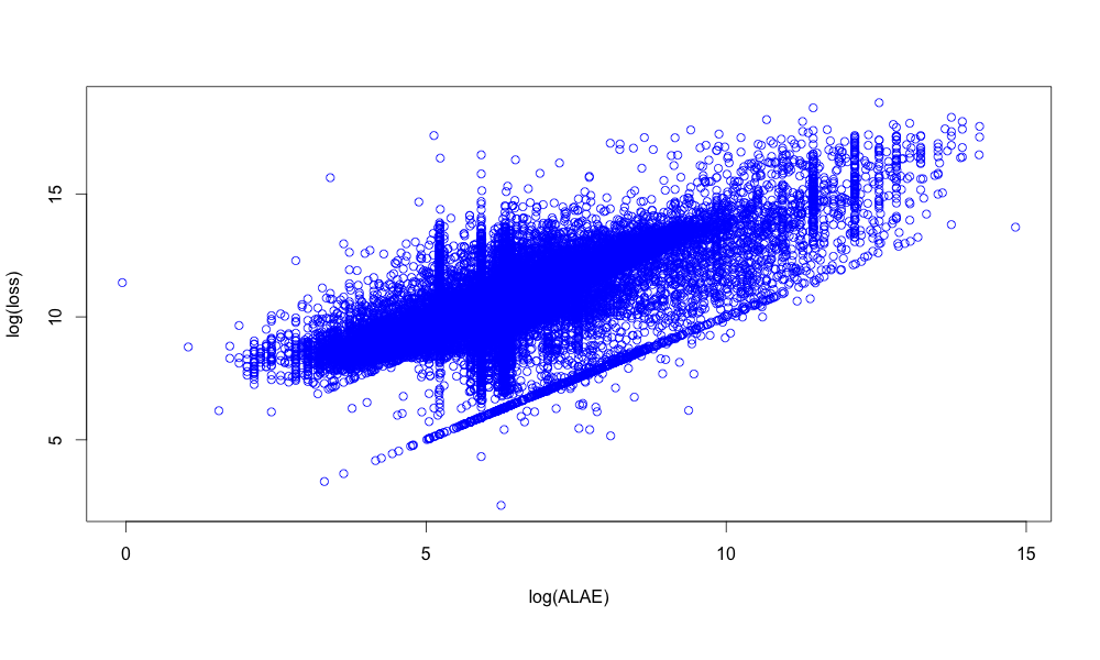
Figure 1. Scatterplot for log ALAE and log Loss: accident insurance data.

Pearson’s Correlation	0.7460
Spearman’s Rho	0.7465
Kendall’s Tau	0.6012
Upper tail dependence	0.6869

Table 8. Empirical dependence measures for Loss ALAE data from accident line.

Referring to the marginal’s estimator in (22), the estimation results for each copula model are found by maximizing (23) and are summarized in Table 9 below.

Model	$\theta$	$\alpha$	$m$	AIC
Gumbel	-	2.3876	-	-32’073
Gumbel Geometric	0.7630	2.2758	-	-32’128
Gumbel Truncated Poisson	0.3133	2.3240	-	-32’104
Gumbel Shifted Poisson	0.1490	2.3276	-	-32’059
Frank	-	8.0774	-	-30’137
Frank Geometric	0.9999	8.0772	-	-30’134
Frank Truncated Poisson	0.0001	8.0773	-	-30’135
Frank Shifted Poisson	0.0001	8.0773	-	-30’135
Student	-	0.8142	1.9805	-32’909
Student Geometric	0.1137	0.5492	1.9992	-38’088
Student Truncated Poisson	0.0001	0.7841	9.6744	-28’672
Student Shifted Poisson	0.0001	0.7885	8.7113	-29’042
Joe	-	3.0967	-	-30’655
Joe Geometric	0.3254	2.3727	-	-33’015
Joe Truncated Poisson	1.8660	2.5885	-	-32’578
Joe Shifted Poisson	0.9537	2.6634	-	-32’411

Table 9. Copula families parameters estimates.

It can be seen that the model which best fits the data is the Student Geometric copula followed by the Joe Geometric copula. We note in passing that the Student copula $Q_{\alpha}$ has an additional parameter $m$ which is the degree of freedom.

5.2. Loss ALAE from general liability insurance

This data set describes the general liability claims associated with their ALAE retrieved from the Insurance Services Office available in the R package. In this respect, the sample consists of 1’466 uncensored data points and 34 censored observations. We refer to Denuit et al. (2006) for more details on the description of the data. Let $X_{i}$ be the $i^{th}$ loss observed and $Y_{i}$ the ALAE associated to the settlement of $X_{i}$. Each loss is associated with a maximum insured claim amount (policy limit) $M$. Thus, the loss variable $X_{i}$ is censored when it exceeds the policy limit $M$. We define the censored indicator of the loss variable by

$$\delta_{i}=\left\{\begin{array}[]{lcl}1&\mbox{if}&X_{i}\leqslant M,\\ 0&\mbox{if}&X_{i}>M,i=1,\ldots,1^{\prime}500.\end{array}\right.$$

Next, we shall use the Kaplan-Meir estimator $\hat{G}_{X}$ to estimate $G_{1}$ and the empirical distribution $\hat{G}_{Y}$ for $G_{2}$ as in (22). In particular, the corresponding pseudo log-likelihood function is given by

(27) $$l(\Theta)=\sum_{i=1}^{n}\Bigl{(}\delta_{i}\ln(c_{\Theta}(U_{1i},U_{2i})+(1-\delta_{i})\ln\Bigl{(}1-\frac{C_{\Theta}(U_{1i},U_{2i})}{\partial U_{2i}}\Bigr{)}\Bigr{)},$$

where $U_{1i}=\frac{n}{n+1}\hat{G}_{X}(x_{i})$ and $U_{2i}=\frac{n}{n+1}\hat{G}_{Y}(y_{i})$ for $i=1,\ldots,n$, see Denuit et al.(2006). By maximizing (27), the resulting estimators of $\Theta$ for the considered copula models are presented in Table 10.

Model	$\theta$	$\alpha$	$m$	AIC
Gumbel	-	1.4284	-	-210.18
Gumbel Geometric	0.5425	1.3127	-	-278.23
Gumbel Truncated Poisson	0.0001	1.4422	-	-360.49
Gumbel Shifted Poisson	0.1410	1.4083	-	-361.20
Frank	-	3.0440	-	-321.44
Frank Geometric	0.7800	2.7464	-	-174.40
Frank Truncated Poisson	0.0001	3.0375	-	-306.40
Frank Shifted Poisson	0.0001	3.0375	-	-306.41
Student	-	0.4642	10.0006	-180.99
Student Geometric	0.7095	0.4252	9.1897	-228.82
Student Truncated Poisson	1	0.4094	13.9922	-271.40
Student Shifted Poisson	1	0.4016	13.9983	-295.42
Joe	-	1.6183	-	-179.00
Joe Geometric	0.4379	1.3864	-	-292.41
Joe Truncated Poisson	0.0607	1.6356	-	-331.21
Joe Shifted Poisson	0.8075	1.4629	-	-361.76

Table 10. Copula families parameters estimates.

Since the Joe Shifted Poisson copula has the the smallest AIC it represents the best model for describing the dependence in the dataset followed by the Gumbel Shifted Poisson copula.

5.3. Danish fire insurance data

The corresponding data set describes the Danish fire insurance claims collected from the Copenhagen Reinsurance Company for the period 1980-1990. It can be retrieved from the following website: $www.ma.hw.ac.uk/\sim mcneil/$. This data set has first been considered by Embrechts et al. (1998) (Example 6.2.9) and explored by Haug et al. (2011). It consists of three components: loss to buildings, loss to contents and loss to profit. However, in this case, we model the dependence between the first two components. The total number of observations is of 1’501. We only consider the observations where both components are non-null. As indicated by the empirical dependence measures in Table 11, the level of dependence between these two losses is low.

Pearson’s Correlation	0.1413
Spearman’s Rho	0.1417
Kendall’s Tau	0.0856
Upper tail dependence	0.1998

Table 11. Dependence measures for the Danish fire insurance.

The estimation results for each copula is summarized in Table 12 below.

Model	$\theta$	$\alpha$	$m$	AIC
Gumbel	-	1.1762	-	-133.18
Gumbel Geometric	0.9999	1.1762	-	-131.17
Gumbel Truncated Poisson	0.0001	1.1762	-	-131.18
Gumbel Shifted Poisson	0.0001	1.1762	-	-131.17
Frank	-	0.8807	-	-29.12
Frank Geometric	0.9999	0.8804	-	-27.12
Frank Truncated Poisson	0.0001	0.8806	-	-27.12
Frank Shifted Poisson	0.0001	0.8805	-	-27.12
Student	-	0.1574	9.5998	-47.86
Student Geometric	0.9999	0.1576	10.0063	-45.84
Student Truncated Poisson	0.0001	0.1570	9.0048	-45.81
Student Shifted Poisson	0.0001	0.1562	8.9833	-45.42
Joe	-	1.3585	-	-204.85
Joe Geometric	0.9999	1.3585	-	-202.83
Joe Truncated Poisson	0.0001	1.3585	-	-202.84
Joe Shifted Poisson	0.0001	1.3585	-	-202.83

Table 12. Copula families parameters estimates.

It can be seen that the model that best fits the data is the Joe copula followed by the Joe Truncated Poisson copula. The Frank mixture copulas and Student mixture copulas are not a good fit for the data as their AIC is higher by far compared to the Gumbel and Joe mixture copulas families.

5.4. Reinsurance premiums

In this section, we examine the effects of the dependence structure on reinsurance premiums by using the proposed copula models. In practice, it is well known that insurance risks dependency has an impact on reinsurance. For instance, Dhaene and Goovaerts (1996) have shown that stop loss premium is greater under the dependence assumption than under the independence case. In what follows, we consider the insurance claims data described in Subsection 5.1 where we denote $X$ the loss variable, $Y$ the associated ALAE and $K$ the number of claims for the next accident year. In addition, two types of reinsurance treaties are analyzed namely:

• Excess-of-loss reinsurance, where the claims from $Y_{i}$ ’s are attributed proportionally to the insurer and the reinsurer. For a given observation $(X_{i},Y_{i})$ the payment for the reinsurer is described as follows, see Cebrian et al. (2003)

  $$g(X_{i},Y_{i},r)=\left\{\begin{array}[]{lcl}0&\mbox{if}&X_{i}\leqslant r,\\ X_{i}-r+\biggl{(}\frac{X_{i}-r}{X_{i}}\biggr{)}Y_{i}&\mbox{if}&X_{i}>r\end{array}\right.$$

  leading to a reinsurance premium of the form

  (29) $$\kappa(r)=\mathbb{E}\left\{K\right\}\mathbb{E}\left\{g(X_{i},Y_{i},r)\right\},$$

  where $r>0$ is the retention level.

• Stop loss reinsurance, where the premium is given by

  (30) $$\pi(d)=\mathbb{E}\left\{\Bigl{(}\sum_{i=1}^{K}(X_{i}+Y_{i})-d\Bigr{)}_{+}\right\}$$

  and $d$ is a positive deductible.

In order to calculate the reinsurance premiums defined above, Monte Carlo simulations have been implemented. Hereof, we assume that $K$ is Poisson distributed with a mean of $156.2$, representing the expected number of claims estimated by the insurance company. Additionally, we use the empirical distributions of $X_{i}$ and $Y_{i}$ for the simulation of the claims amount. Regarding the dependence model, the following copulas are considered: independent copula, Joe copula, Geometric Joe Copula, Truncated Poisson Joe copula and the Shifted Poisson Joe copula where the parameters are summarized in Table 9. The following steps summarize the implemented pseudo-algorithm:

• Step 1: Generate the number of claims $K\sim Poisson(156.2)$.

• Step 2: Simulate $(u_{i},v_{i}),i=1,\ldots,K$ from the considered copula $C$.

• Step 3: Generate the loss and ALAE claims as follows

  $$(x_{i}=\hat{F}_{X,n}^{-1}(u_{i}),y_{i}=\hat{F}_{Y,n}^{-1}(v_{i})),i=1,\ldots,K,$$

  where $\hat{F}_{X,n}^{-1}$ and $\hat{F}_{Y,n}^{-1}$ are the inverse of the empirical df of $X$ and $Y$ respectively, with

  $$\hat{F}_{X,n}(x)=\frac{1}{n}\sum_{i=1}^{n}\mathbf{1}(X_{i}\leq x),\quad\hat{F}_{Y,n}(y)=\frac{1}{n}\sum_{i=1}^{n}\mathbf{1}(Y_{i}\leq y).$$

• Step 4: Calculate the reinsurance premiums $\kappa^{b}(r)$ and $\pi^{b}(d)$ as in (29) and (30) respectively.

• Step 5: Step 1 -Step 4 are repeated $B$ times and the estimators of the reinsurance premiums are given by

  $$\hat{\kappa}(r)=\frac{1}{B}\sum_{b=1}^{B}\kappa^{b}(r),\quad\hat{\pi}(d)=\frac{1}{B}\sum_{b=1}^{B}\pi^{b}(d).$$

The estimation results presented in Table 13 are obtained from repeating Step 1 -Step 4 100’000 times. These amounts are expressed in CHF million.

	$\hat{\kappa}(r)$			$\hat{\pi}(d)$
Copula model	$r=1$	$r=5$	$r=10$	$d=10$	$d=20$	$d=30$
Independent	13.1137	6.5692	3.0971	14.7530	7.5145	3.5738
Joe	13.6950	6.7776	3.2396	15.1056	7.7691	3.8233
Joe Geometric	13.4483	6.7365	3.1619	14.8975	7.6797	3.7177
Joe Truncated Poisson	13.4038	6.7183	3.0929	14.8016	7.6698	3.6493
Joe Shifted Poisson	13.4776	6.6789	3.1081	14.9250	7.6266	3.6702

Table 13. Reinsurance premiums with respect to copula models.

Table 13 shows that the reinsurance premiums $\hat{\kappa}(r)$ and $\hat{\pi}(d)$ are lower under the independence hypothesis. Hence, the portfolio is less risky when the loss variable $X_{i}$ and the ALAE variable $Y_{i}$ are assumed to be independent. Furthermore, when the retention limit $r$ increases for the excess of loss treaty, the reinsurance premiums estimates $\hat{\kappa}(r)$ under the Joe mixture copula models tend to the estimated values under the independence assumption. Conversely, for the stop loss treaty, the higher the deductible $d$ the higher the deviation from the independence hypothesis.
Furthermore, by comparing the results for each copula model, it can be seen that the Joe copula generates the highest reinsurance premiums. This result is expected given that the strongest dependence structure is obtained under the Joe copula. On the other hand, the weakest dependence model for this data is observed under the Joe truncated Poisson copula as the reisurance premiums $\hat{\kappa}(r)$ and $\hat{\pi}(d)$ are the smallest for different values of $r$ and $d$.

6. Appendix

6.1. Proofs

Derivation of (25)-(26): We show first (7). The corresponding joint density $c$ of the df $C$ is given by

(31) $$c(u_{1},u_{2})=\frac{\partial C(u_{1},u_{2})}{\partial u_{1}\partial u_{2}}=\frac{\partial L_{\Lambda}(-\ln Q_{\alpha}(v_{1},v_{2}))}{\partial u_{1}\partial u_{2}},$$

where

$$C(v_{1},v_{2})=L_{\Lambda}(-\ln Q_{\alpha}(v_{1},v_{2})),\quad{\color[rgb]{0.,0.,0.}v_{i}=e^{-L^{-1}_{\Lambda}(u_{i})}},\quad i=1,2.$$

In view of (31), the partial derivative of $C$ with respect to $u_{1}$ is

$$\frac{\partial L_{\Lambda}(-\ln Q_{\alpha}(v_{1},v_{2}))}{\partial u_{1}}=\frac{1}{Q_{\alpha}(v_{1},v_{2})}L^{\prime}_{\Lambda}(-\ln Q_{\alpha}(v_{1},v_{2}))\frac{-\partial Q_{\alpha}(v_{1},v_{2})}{\partial v_{1}}\frac{\partial v_{1}}{\partial u_{1}}$$

leading to

$$c(u_{1},u_{2}) = \frac{\partial}{\partial v_{2}}\Biggl{(}\frac{\partial L_{\Lambda}(-\ln Q_{\alpha}(v_{1},v_{2}))}{\partial u_{1}}\Biggr{)}\frac{\partial v_{1}}{\partial u_{1}}\frac{\partial v_{2}}{\partial u_{2}}$$

$$= \frac{\partial v_{2}}{\partial u_{2}}\Biggl{(}L^{\prime\prime}_{\Lambda}(-\ln Q_{\alpha}(v_{1},v_{2}))\frac{\frac{\partial Q_{\alpha}(v_{1},v_{2})}{\partial v_{1}}\frac{\partial Q_{\alpha}(v_{1},v_{2})}{\partial v_{2}}}{Q_{\alpha}^{2}(v_{1},v_{2})}$$

$$+L^{\prime}_{\Lambda}(-\ln Q_{\alpha}(v_{1},v_{2}))\frac{\frac{-\partial^{2}Q_{\alpha}(v_{1},v_{2})}{\partial v_{1}\partial v_{2}}Q_{\alpha}(v_{1},v_{2})+\frac{\partial Q_{\alpha}(v_{1},v_{2})}{\partial v_{1}}\frac{\partial Q_{\alpha}(v_{1},v_{2})}{\partial v_{2}}}{Q_{\alpha}^{2}(v_{1},v_{2})}\Biggr{)}$$

$$= \frac{\frac{\partial v_{1}}{\partial u_{1}}\frac{\partial v_{2}}{\partial u_{2}}}{Q_{\alpha}^{2}(v_{1},v_{2})}\Biggl{(}\Bigl{(}L^{\prime\prime}_{\Lambda}(-\ln Q_{\alpha}(v_{1},v_{2}))+L^{\prime}_{\Lambda}(-\ln Q_{\alpha}(v_{1},v_{2}))\Bigr{)}\frac{\partial Q_{\alpha}(v_{1},v_{2})}{\partial v_{1}}\frac{\partial Q_{\alpha}(v_{1},v_{2})}{\partial v_{2}}$$

$$-L^{\prime}_{\Lambda}(-\ln Q_{\alpha}(v_{1},v_{2}))Q_{\alpha}(v_{1},v_{2})\frac{\partial^{2}Q_{\alpha}(v_{1},v_{2})}{\partial v_{1}\partial v_{2}}\Biggr{)}.$$

We derive next the pdf $c_{\Theta}$ in (25): In this case, $\Lambda$ follows a shifted Poisson distribution. In view of (7), we need to compute at first the following components:

$$L^{\prime}_{\Lambda}(-\ln Q_{\alpha}(v_{1},v_{2})) = -e^{-\theta(1-Q_{\alpha}(v_{1},v_{2}))}Q_{\alpha}(v_{1},v_{2})(1+\theta Q_{\alpha}(v_{1},v_{2})),$$

$$L^{\prime\prime}_{\Lambda}(-\ln Q_{\alpha}(v_{1},v_{2})) = e^{-\theta(1-Q_{\alpha}(v_{1},v_{2}))}Q_{\alpha}(v_{1},v_{2})(1+3\theta Q_{\alpha}(v_{1},v_{2})+\theta^{2}Q_{\alpha}^{2}(v_{1},v_{2})),$$

where for $i=1,2$, $v_{i}=e^{-L^{-1}_{\Lambda}(u_{i})}$ which implies $u_{i}=v_{i}e^{-\theta(1-v_{i})}$ and thus $\frac{\partial v_{i}}{\partial u_{i}}=\frac{e^{-\theta(1-v_{i})}}{1+\theta v_{i}}.$ By replacing these components into (7), we have

$$c_{\Theta}(u_{1},u_{2}) = \frac{1}{Q_{\alpha}(v_{1},v_{2})^{2}}\frac{e^{\theta(2-v_{1}-v_{2})}}{(1+\theta v_{1})(1+\theta v_{2})}\Biggl{[}\Bigl{(}e^{-\theta(1-Q_{\alpha}(v_{1},v_{2}))}Q_{\alpha}(v_{1},v_{2})(1+3\theta Q_{\alpha}(v_{1},v_{2})+\theta^{2}Q_{\alpha}^{2}(v_{1},v_{2}))$$

$$-e^{-\theta(1-Q_{\alpha}(v_{1},v_{2}))}Q_{\alpha}(v_{1},v_{2})(1+\theta Q_{\alpha}(v_{1},v_{2})\Bigr{)}\frac{\partial Q_{\alpha}(v_{1},v_{2})}{\partial v_{1}}\frac{\partial Q_{\alpha}(v_{1},v_{2})}{\partial v_{2}}$$

$$+e^{-\theta(1-Q_{\alpha}(v_{1},v_{2}))}Q_{\alpha}(v_{1},v_{2})(1+\theta Q_{\alpha}(v_{1},v_{2}))Q_{\alpha}(v_{1},v_{2})\frac{\partial^{2}Q_{\alpha}(v_{1},v_{2})}{\partial v_{1}\partial v_{2}}\Biggr{]}$$

$$= \frac{1}{Q_{\alpha}(v_{1},v_{2})^{2}}\frac{e^{\theta(2-v_{1}-v_{2})}}{(1+\theta v_{1})(1+\theta v_{2})}\times$$

$$\Biggl{[}e^{-\theta(1-Q_{\alpha}(v_{1},v_{2}))}Q_{\alpha}(v_{1},v_{2})\Bigl{(}1+3\theta Q_{\alpha}(v_{1},v_{2})+\theta^{2}Q_{\alpha}^{2}(v_{1},v_{2})-1-\theta Q_{\alpha}(v_{1},v_{2})\Bigr{)}\frac{\partial Q_{\alpha}(v_{1},v_{2})}{\partial v_{1}}\frac{\partial Q_{\alpha}(v_{1},v_{2})}{\partial v_{2}}$$

$$+e^{-\theta(1-Q_{\alpha}(v_{1},v_{2}))}Q_{\alpha}^{2}(v_{1},v_{2})(1+\theta Q_{\alpha}(v_{1},v_{2}))\frac{\partial^{2}Q_{\alpha}(v_{1},v_{2})}{\partial v_{1}\partial v_{2}}\Biggr{]}$$

$$= \frac{1}{Q(v_{1},v_{2})^{2}}\frac{e^{\theta(2-v_{1}-v_{2})}}{(1+\theta v_{1})(1+\theta v_{2})}\times$$

$$\Biggl{[}e^{-\theta(1-Q_{\alpha}(v_{1},v_{2}))}Q_{\alpha}(v_{1},v_{2})\Bigl{(}2\theta Q_{\alpha}(v_{1},v_{2})+\theta^{2}Q_{\alpha}^{2}(v_{1},v_{2})\Bigr{)}\frac{\partial Q_{\alpha}(v_{1},v_{2})}{\partial v_{1}}\frac{\partial Q_{\alpha}(v_{1},v_{2})}{\partial v_{2}}$$

$$+e^{-\theta(1-Q_{\alpha}(v_{1},v_{2}))}Q_{\alpha}^{2}(v_{1},v_{2})(1+\theta Q_{\alpha}(v_{1},v_{2}))\frac{\partial^{2}Q_{\alpha}(v_{1},v_{2})}{\partial v_{1}\partial v_{2}}\Biggr{]}$$

$$= \frac{1}{Q(v_{1},v_{2})^{2}}\frac{e^{\theta(2-v_{1}-v_{2})}}{(1+\theta v_{1})(1+\theta v_{2})}\times$$

$$\Biggl{[}e^{-\theta(1-Q_{\alpha}(v_{1},v_{2}))}Q_{\alpha}^{2}(v_{1},v_{2})\Bigl{(}2\theta+\theta^{2}Q_{\alpha}(v_{1},v_{2})\Bigr{)}\frac{\partial Q_{\alpha}(v_{1},v_{2})}{\partial v_{1}}\frac{\partial Q_{\alpha}(v_{1},v_{2})}{\partial v_{2}}$$

$$+e^{-\theta(1-Q_{\alpha}(v_{1},v_{2}))}Q_{\alpha}^{2}(v_{1},v_{2})(1+\theta Q_{\alpha}(v_{1},v_{2}))\frac{\partial^{2}Q_{\alpha}(v_{1},v_{2})}{\partial v_{1}\partial v_{2}}\Biggr{]}$$

$$= \frac{1}{Q(v_{1},v_{2})^{2}}\frac{e^{\theta(2-v_{1}-v_{2})}}{(1+\theta v_{1})(1+\theta v_{2})}e^{-\theta(1-Q_{\alpha}(v_{1},v_{2}))}Q_{\alpha}^{2}(v_{1},v_{2})\times$$

$$\Biggl{[}\theta\frac{\partial Q_{\alpha}(v_{1},v_{2})}{\partial v_{1}}\frac{\partial Q_{\alpha}(v_{1},v_{2})}{\partial v_{2}}\Bigl{(}2+\theta Q_{\alpha}(v_{1},v_{2})\Bigr{)}+(1+\theta Q_{\alpha}(v_{1},v_{2}))\frac{\partial^{2}Q_{\alpha}(v_{1},v_{2})}{\partial v_{1}\partial v_{2}}\Biggr{]}$$

$$= \frac{e^{\theta(2-v_{1}-v_{2})}e^{\theta(Q_{\alpha}(v_{1},v_{2})-1)}}{(1+\theta v_{1})(1+\theta v_{2})}\Biggl{[}\frac{\partial^{2}Q_{\alpha}(v_{1},v_{2})}{\partial v_{1}\partial v_{2}}(1+\theta Q_{\alpha}(v_{1},v_{2}))+\theta\frac{\partial Q_{\alpha}(v_{1},v_{2})}{\partial v_{1}}\frac{\partial Q_{\alpha}(v_{1},v_{2})}{\partial v_{2}}(2+\theta Q_{\alpha}(v_{1},v_{2}))\Biggr{]}.$$

Next, we show (26): Since $\Lambda$ follows a truncated Poisson distribution, in light of (7), the joint density $c_{\Theta}$ is expressed in terms of (set $\eta_{\theta}=e^{-\theta}/(1-e^{-\theta})$)

$$L^{\prime}_{\Lambda}(-\ln Q_{\alpha}(v_{1},v_{2})) = -\eta_{\theta}\theta Q_{\alpha}(v_{1},v_{2})e^{\theta Q_{\alpha}(v_{1},v_{2})},$$

$$L^{\prime\prime}_{\Lambda}(-\ln Q_{\alpha}(v_{1},v_{2})) = \eta_{\theta}\theta Q_{\alpha}(v_{1},v_{2})e^{\theta Q_{\alpha}(v_{1},v_{2})}(1+\theta Q_{\alpha}(v_{1},v_{2})),$$

where for $i=1,2$, $v_{i}=e^{-L^{-1}_{\Lambda}(u_{i})}$ and $u_{i}=\frac{e^{-\theta}}{1-e^{-\theta}}(v_{i}^{\theta}-1)$ with $\frac{\partial v_{i}}{\partial u_{i}}=\frac{1-e^{-\theta}}{\theta}e^{\theta(1-v_{i})}.$ By substituting the above components in the joint density expressed in (7), we obtain

$$c_{\Theta}(u_{1},u_{2}) = \Biggl{(}\frac{1-e^{-\theta}}{\theta}\Biggr{)}^{2}\frac{e^{\theta(2-v_{1}-v_{2})}}{Q_{\alpha}^{2}(v_{1},v_{2})}\Biggl{[}\Biggl{(}\eta_{\theta}\theta Q_{\alpha}(v_{1},v_{2})e^{\theta Q(v_{1},v_{2})}(1+\theta Q_{\alpha}(v_{1},v_{2}))$$

$$-\eta_{\theta}\theta Q_{\alpha}(v_{1},v_{2})e^{\theta Q_{\alpha}(v_{1},v_{2})}\Biggr{)}\frac{\partial Q_{\alpha}(v_{1},v_{2})}{\partial v_{1}}\frac{\partial Q_{\alpha}(v_{1},v_{2})}{\partial v_{2}}$$

$$+\eta_{\theta}\theta Q_{\alpha}(v_{1},v_{2})e^{\theta Q_{\alpha}(v_{1},v_{2})}Q_{\alpha}(v_{1},v_{2})\frac{\partial^{2}Q_{\alpha}(v_{1},v_{2})}{\partial v_{1}\partial v_{2}}\Biggr{]}$$

$$= (1-e^{-\theta})e^{\theta[1-v_{1}-v_{2}+Q_{\alpha}(v_{1},v_{2})]}\Biggl{(}\frac{\partial Q_{\alpha}(v_{1},v_{2})}{\partial v_{1}}\frac{\partial Q_{\alpha}(v_{1},v_{2})}{\partial v_{2}}+\frac{1}{\theta}\frac{\partial^{2}Q_{\alpha}(v_{1},v_{2})}{\partial v_{1}\partial v_{2}}\Biggr{)}.$$

$\Box$
Proof of Proposition 3.1 Since $G$ has Fréchet marginals, by assumption (11), we have that

$$\lim_{n\to\infty}G^{n}(nx,ny)=\mathcal{G}(x,y),\quad x,y\in(0,\infty),$$

where $\mathcal{G}$ has copula $Q_{A}$ and thus $\tau(\mathcal{G})=\tau(Q_{{A}})$. We have thus with $F_{n}(x,y)=\mathbb{E}\left\{G^{\Lambda_{n}}(x,y)\right\}$ using further (9)

(32) $$\lim_{n\to\infty}F_{n}(nx_{n},ny_{n})=\lim_{n\to\infty}\mathbb{E}\left\{G^{n\frac{\Lambda_{n}}{n}}(nx_{n},ny_{n})\right\}=\mathcal{G}(x,y),\quad x,y\in(0,\infty)$$

for any $x_{n},y_{n}$ such that $\lim_{n\to\infty}x_{n}=x$ and $\lim_{n\to\infty}y_{n}=y$. Consequently,

$$\tau(C_{n}) = 4\int_{(0,\infty)^{2}}F_{n}(x,y)\,dF_{n}(x,y)-1$$

$$= 4\int_{(0,\infty)^{2}}F_{n}(nx,ny)\,dF_{n}(nx,ny)-1$$

$$\to 4\int_{(0,\infty)^{2}}\mathcal{G}(x,y)\,d\mathcal{G}(x,y)-1,\quad n\to\infty$$

$$= \tau(\mathcal{G}),$$

where the convergence above follows by Lemma 4.2 in Hashorva (2007) (see also Resnick and Zeber (2013) and Kulik and Soulier (2015) for more general results). Next, the convergence in (32) implies

$$\lim_{n\to\infty}F_{ni}(ns_{n})=\lim_{n\to\infty}\mathbb{E}\left\{G^{n\frac{\Lambda_{n}}{n}}_{i}(ns_{n})\right\}=\mathcal{G}_{i}(s),\quad s\in(0,\infty),i=1,2$$

for any $s_{n},n\geq 1$ such that $\lim_{n\to\infty}s_{n}=s$, where $F_{ni},G_{i},\mathcal{G}_{i}$ is the $i$th marginal df of $F_{n},G$, and $\mathcal{G}$, respectively. Hence, with similar arguments as above, we have

$$\rho_{S}(C_{n}) = 12\int_{(0,\infty)^{2}}F_{n}(x,y)\,dF_{n1}(x)dF_{n2}(y)-3$$

$$= 12\int_{(0,\infty)^{2}}F_{n}(nx,ny)\,dF_{n1}(nx)dF_{n2}(nx)-3$$

$$\to 12\int_{(0,\infty)^{2}}\mathcal{G}(x,y)\,d\mathcal{G}_{1}(x)d\mathcal{G}_{2}(x)-3,\quad n\to\infty$$

$$= \rho_{S}(\mathcal{G})$$

establishing the proof. $\Box$

Proof of Proposition 3.2 For $v=e^{-L_{\Lambda}^{-1}(1-u)}$ we have

$$1-L_{\Lambda}(-\ln v)\sim u,\quad u\downarrow 0,\quad\lim_{u\downarrow 0}v=1.$$

By the assumption that $\mathbb{E}\left\{\Lambda\right\}$ is finite we have

(33) $$1-L_{\Lambda}(t)\sim-L_{\Lambda}^{\prime}(0)t=\mathbb{E}\left\{\Lambda\right\}t,\quad t\to 0.$$

Since further

$$\mu_{Q}=2-\lim_{u\downarrow 0}\frac{Q(1-u,1-u)}{u}=2-\lim_{v\uparrow 1}\frac{\ln Q(v,v)}{\ln v}$$

and $\lim_{v\uparrow 1}Q(v,v)=1,$ then using (6) and (33) we obtain

$$\mu_{C} = 2-\lim_{u\downarrow 0}u^{-1}[1-C(1-u,1-u))]$$

$$= 2-\lim_{u\downarrow 0}u^{-1}\Bigl{[}1-L_{\Lambda}\bigl{(}-\ln Q(v,v)\bigr{)}\Bigr{]}$$

$$= 2-\lim_{u\downarrow 0}\frac{1-L_{\Lambda}\bigl{(}-\ln Q(v,v)\bigr{)}}{1-L_{\Lambda}(-\ln v)}$$

$$= 2-\lim_{v\uparrow 1}\frac{\ln Q(v,v)}{\ln v}$$

$$= 2-[2-\mu_{Q}]=\mu_{Q},$$

hence the first claim follows. Next, in view of (16) we have

$$\lim_{n\to\infty}n[1-G(nx,ny)]=-\ln H(x,y),\quad x,y\in(0,\infty),$$

hence as $n\to\infty$

$$n[1-G(nx,ny)]\sim\frac{1-G(nx,ny)}{1-G(n,n)}\sim-\ln H(x,y),\quad x,y\in(0,\infty).$$

Let $a_{n},n\geq 1$ be non-negative constants such that $\lim_{n\to\infty}a_{n}=\infty$. By the above and (33)

$$n[1-F(a_{n}x,a_{n}y)] = n[1-L_{\Lambda}(-\ln G(a_{n}x,a_{n}y))]\sim\mathbb{E}\left\{\Lambda\right\}n(-\ln G(a_{n}x,a_{n}y))$$

as $n\to\infty$. Setting now $a_{n}=\mathbb{E}\left\{\Lambda\right\}n$ we have thus as $n\to\infty$

$$n[1-F(a_{n}x,a_{n}y)] \sim a_{n}\frac{1-F(a_{n}x,a_{n}y)}{\mathbb{E}\left\{\Lambda\right\}}$$

$$= a_{n}\frac{1-L_{\Lambda}(-\ln G(a_{n}x,a_{n}y))}{\mathbb{E}\left\{\Lambda\right\}}$$

$$\sim a_{n}(-\ln G(a_{n}x,a_{n}y))$$

$$\sim a_{n}[1-G(a_{n}x,a_{n}y)[$$

$$\sim \mathbb{E}\left\{\Lambda\right\}\Bigl{(}-\ln H(x\mathbb{E}\left\{\Lambda\right\},y\mathbb{E}\left\{\Lambda\right\})\Bigr{)}$$

$$= -\ln H(x,y)$$

establishing the proof. $\Box$

For our study, we consider several copula families for $Q_{\alpha}$, which are described hereafter.

6.2. Gumbel Copula

The df of a Gumbel copula with a dependence parameter $\alpha\geq 1$ is given by

$$Q_{\alpha}(v_{1},v_{2})=\exp\biggl{(}-\Bigl{(}(-\ln v_{1})^{\alpha}+(-\ln v_{2})^{\alpha}\Bigr{)}^{\frac{1}{\alpha}}\biggl{)}$$

by differentiating $Q_{\alpha}(v_{1},v_{2})$ with respect to $v_{1}$ we have

$$\frac{\partial Q_{\alpha}(v_{1},v_{2})}{\partial v_{1}}=\frac{1}{v_{1}}(-\ln v_{1})^{\alpha-1}\Biggl{(}(-\ln v_{1})^{\alpha}+(-\ln v_{2})^{\alpha}\Biggr{)}^{\frac{1}{\alpha-1}}e^{-\Bigl{(}(-\ln v_{1})^{\alpha}+(-\ln v_{2})^{\alpha}\Bigr{)}^{\frac{1}{\alpha}}},$$

and the corresponding joint density is expressed as follows

$$q_{\alpha}(v_{1},v_{2}) = \frac{(-\ln v_{1})^{\alpha-1}(-\ln v_{2})^{\alpha-1}}{v_{1}v_{2}}\Bigl{(}a^{\frac{2}{\alpha}-2}+(\alpha-1)a^{\frac{1}{\alpha}-2}\Bigr{)}e^{-a^{\frac{1}{\alpha}}},$$

where $a=(-\ln v_{1})^{\alpha}+(-\ln v_{2})^{\alpha}$.

6.3. Frank Copula

The df of a Frank copula with a dependence parameter $\alpha\neq 0$ is of the form

$$Q_{\alpha}(v_{1},v_{2})=\frac{-1}{\alpha}\ln\Bigl{(}1+\frac{(e^{-\alpha v_{1}}-1)(e^{-\alpha v_{2}}-1)}{e^{-\alpha}-1}\Bigr{)},$$

which yields the partial derivative of $Q_{\alpha}(v_{1},v_{2})$ with respect to $v_{1}$ as follows

$$\frac{\partial Q_{\alpha}(v_{1},v_{2})}{\partial v_{1}}=\frac{e^{-\alpha v_{1}}(e^{-\alpha v_{2}}-1)}{(e^{-\alpha}-1)+(e^{-\alpha v_{1}}-1)(e^{-\alpha v_{2}}-1)}$$

and the associated pdf is given by

$$q_{\alpha}(v_{1},v_{2}) = \frac{\alpha(1-e^{-\alpha})e^{-\alpha(v_{1}+v_{2})}}{\Bigl{(}(1-e^{-\alpha})-(1-e^{-\alpha v_{1}})(1-e^{-\alpha v_{2}})\Bigr{)}^{2}}.$$

6.4. Joe copula

The Joe copula with dependence parameter $\alpha\geq 1$ has df

$$Q_{\alpha}(v_{1},v_{2})=1-\Bigl{(}(1-v_{1})^{\alpha}+(1-v_{2})^{\alpha}-(1-v_{1})^{\alpha}(1-v_{2})^{\alpha}\Bigr{)}^{\frac{1}{\alpha}}.$$

Deriving $Q_{\alpha}(v_{1},v_{2})$ with respect to $v_{1}$ we obtain

$$\frac{\partial Q_{\alpha}(v_{1},v_{2})}{\partial v_{1}}=(1-v_{1})^{\alpha-1}(1-(1-v_{2})^{\alpha})\Bigl{(}(1-v_{1})^{\alpha}+(1-v_{2})^{\alpha}-(1-v_{1})^{\alpha}(1-v_{2})^{\alpha}\Bigr{)}^{\frac{1}{\alpha}-1}.$$

The associated pdf is obtained by differentiating $Q_{\alpha}(v_{1},v_{2})$ with respect to $v_{1}$ and $v_{2}$ leading to

$$q_{\alpha}(v_{1},v_{2}) = (1-v_{1})^{\alpha-1}(1-v_{2})^{\alpha-1}\Bigl{(}\alpha-1+b\Bigr{)}b^{\frac{1}{\alpha}-2},$$

where $b=(1-v_{2})^{\alpha}-(1-v_{1})^{\alpha}(1-v_{2})^{\alpha}$.

6.5. Student Copula

Let $t_{m}$ be the df of a Student random variable with degree of freedom $m$ and write $t_{m}^{-1}$ for its inverse. The df of the Student copula, with correlation $\alpha\in(-1,1)$ and degree of freedom $m>0$ can be expressed as follows

$$Q_{\alpha,m}(v_{1},v_{2}) = t_{\alpha,m}(t_{m}^{-1}(v_{1}),t_{m}^{-1}(v_{2}))$$

$$= \int_{-\infty}^{t_{m}^{-1}(v_{1})}\int_{-\infty}^{t_{m}^{-1}(v_{2})}\frac{1}{\sqrt{2\pi(1-\alpha^{2})}}\Bigl{(}1+\frac{s^{2}-2\alpha st+t^{2}}{m(1-\alpha^{2})}\Bigr{)}^{-(m+2)/2}dsdt.$$

Its partial derivative with respect to $v_{1}$ is given by

$$\frac{\partial Q_{\alpha}(v_{1},v_{2})}{\partial v_{1}}=t_{m+1}\Biggl{(}\frac{t^{-1}_{m}(v_{2})-\alpha t^{-1}_{m}(v_{1})}{\sqrt{\frac{(m+(t^{-1}_{m}(v_{1}))^{2})(1-\alpha^{2})}{m+1}}}\Biggr{)},$$

whereas the corresponding pdf is

$$q_{\alpha,m}(v_{1},v_{2}) = \frac{1}{2\pi\sqrt{1-\alpha^{2}}}\frac{1}{k(t^{-1}_{m}(v_{1}))k(t^{-1}_{m}(v_{2}))}\Bigl{(}1+\frac{{t^{-1}_{m}(v_{1})}^{2}+{t^{-1}_{m}(v_{2})}^{2}-2\alpha t^{-1}_{m}(v_{1})t^{-1}_{m}(v_{2})}{m(1-\alpha^{2})}\Bigr{)}^{-\frac{m+2}{2}},$$

where for $i=1,2$

$$k(t^{-1}_{m}(v_{i}))=\frac{\Gamma(\frac{m+1}{2})}{\Gamma(\frac{m}{2})\sqrt{\pi m}}\Bigl{(}1+\frac{t^{-1}_{m}(v_{i})^{2}}{m}\Bigr{)}^{-\frac{m+1}{2}}.$$

Acknowledgments. Thanks to reviewers and the Editor for several suggestions. E. Hashorva is partially supported by the Swiss National Science Foundation grants 200021-13478, 200021-140633/1. G. Ratovomirija is partially supported by the project RARE -318984 (an FP7 Marie Curie IRSES Fellowship) and Vaudoise Assurances.

References

- [1] Ammeter, H. (1964). Note concerning the distribution function of the total loss excluding the largest individual claims. Astin Bulletin, 3(02), 132–143.
- [2] Asimit, A.V. and Chen, Y. (2015). Asymptotic results for conditional measures of association of a random sum. Insurance: Mathematics & Economics, 60, 11–18.
- [3] Aulbach, S. , Falk, M, Hofmann, M. & Zott, M. (2015). Max-stable processes and the functional -norm revisited. Extremes, 18(2), 191–212.
- [4] Aulbach, S. , Falk, M. & Zott, M. (2015). The space of -norms revisited. Extremes, 18(1), 85–97.
- [5] Bücher, A. & Segers, J. (2014). Extreme value copula estimation based on block maxima of a multivariate stationary time series. Extremes, 17(3), 495–528.
- [6] Cebrian, A.C. , Denuit, M. & Lambert, P. (2003). Analysis of bivariate tail dependence using extreme value copulas: An application to the SOA medical large claims database. Belgian Actuarial Journal, 3(1), 33–41.
- [7] Denuit, M., Dhaene, J., Goovaerts, M. & Kass, R. (2006). Actuarial Theory for Dependent Risks: Measures, Orders and Models. Chichester: John Wiley & Sons.
- [8] Denuit, M., Purcaruff, O. & Van Keilegorni, I. (2006). Bivariate Archimedean copula models for censored data in non-life insurance. Journal of Actuarial Practice, 13.
- [9] Dhaene, J. & Goovaerts, M.J. (1996). Dependency of risks and stop-loss order. Astin Bulletin, 26(02), 201–212.
- [10] Embrechts, P. (2009). Copulas: a personal view. Journal of Risk and Insurance, 76(3), 639–650.
- [11] Embrechts, P., Klüppelberg, C. & Mikosch, T. (1998). Modelling extremal events for insurance and finance. Astin Bulletin, 28(02), 285–286.
- [12] Falk, M., Hüsler, J. & Reiss, R.D. (2010). Laws of Small Numbers: Extremes and Rare Events. Springer Science & Business Media.
- [13] Genest, C., Gendron, M. & Bourdeau-Brien, M. (2009). The advent of copulas in finance. The European Journal of Finance, 15(7-8), 609–618.
- [14] Genest, C., Ghoudi, K. & Rivest, L.P. (1995). A semiparametric estimation procedure of dependence parameters in multivariate families of distributions. Biometrika, 82(3), 543–552.
- [15] Hashorva, E. (2007). Extremes of conditioned elliptical random vectors. Journal of Multivariate Analysis, 98(8), 1583–1591.
- [16] Haug, S., Klüppelberg, C. & Peng, L. (2011). Statistical models and methods for dependence in insurance data. Journal of the Korean Statistical Society, 40(2), 125–139.
- [17] Kim, G., Silvapulle, M.J. & Silvapulle, P. (2007). Comparison of semi-parametric and parametric methods for estimating copulas. Computational Statistics and Data Analysis, 51(6), 2836–2850.
- [18] Kulik, R. & Soulier, P. (2015). Heavy tailed time series with extremal independence. Extremes, 18(2), 273–299.
- [19] Molchanov, I. (2008). Convex geometry of max-stable distributions. Extremes, 11(3), 235–259.
- [20] Nelsen, R.B. (1999). An Introduction To Copulas . New York: Springer-Verlag.
- [21] Oakes, D. (1989). Bivariate survival models induced by frailties. Journal of the American Statistical Association, 84(406), 487–493.
- [22] Peng, L. (2014). Joint tail of ECOMOR and LCR reinsurance treaties. Insurance: Mathematics & Economics, 58, 116–120.
- [23] Resnick, S.I. & Zeber, D. (2013). Asymptotics of Markov kernels and the tail chain. Advances in Applied Probability, 45(1), 186–213.
- [24] Zhang , K. & Lin, J. (2016). A new class of copulas involved geometric distribution: Estimation and applications. Insurance: Mathematics & Economics, 66, 1–10.