Potentials and Limits to Basin Stability Estimation

Abstract

Stability assessment methods for dynamical systems have recently been complemented by basin stability and derived measures, i.e. probabilistic statements whether systems remain in a basin of attraction given a distribution of perturbations. This requires numerical estimation via Monte-Carlo sampling and integration of differential equations. Here, we analyze the applicability of basin stability to systems with basin geometries challenging for this numerical method, having fractal basin boundaries and riddled or intermingled basins of attraction. We find that numerical basin stability estimation is still meaningful for fractal boundaries but reaches its limits for riddled basins with holes.

Going back to the path-breaking ideas of Aleksandr M. Lyapunov, dynamical systems are said to be stable if small variations of the initial conditions lead to small reactions of a system, i.e. small perturbations cannot substantially alter the system’s state. This is commonly a statement about the asymptotic behaviour, allowing for large transient deviations if only the system eventually returns to the initial state. Multistable systems with several attractors add another subtlety to the problem: perturbations may lead to switching from one attractor to another, substantially altering asymptotic behaviour (Pisarchik and Feudel, 2014). While infinitesimal perturbations on an attractor have local effects well-studied in the theory of asymptotic stability, finite (including large) perturbations can be critical by causing non-local effects like the transition to another attractor.

A direct stability method are Lyapunov functions (Lyapunov, 1907; Hahn, 1958; Malisoff and Mazenc, 2009), which decrease along trajectories and have local minima on attractors. Finding Lyapunov functions is, however, difficult in high-dimensional multi-stable systems, although there are recent approaches to determine them from radial basis functions (e.g. (Giesl et al., 2016)).

Here, we pursue an alternative approach to consider non-local perturbations termed basin stability $S_{\mathcal{B}}$. The central idea (Menck et al., 2013, 2014) is to use a kind of volume of the basin of attraction to quantify the stability of attractors in multi-stable systems subject to a given distribution of perturbations. An advantage of this measure is that it can be efficiently estimated even in high-dimensional systems and as an intuitive interpretation as a probability to return to an attractor, but it relies on the correct identification of the asymptotic behaviour for a Monte Carlo sample of initial conditions. Basin stability and derived concepts have been successfully applied recently (Rodrigues et al., 2016), e.g. for power grids (Kim et al., 2015, 2016; Menck et al., 2014; Schmietendorf et al., 2014), chimera states (Martens et al., 2016), explosive synchronization (Zou et al., 2014) delayed dynamics (Leng et al., 2016) and resilience measures (Mitra et al., 2015).

In numerical simulations, it can be difficult to correctly identify the asymptotic behaviour and determine the attractors. The basin of attraction can practically be defined as the set of all states that enter and stay in some trapping region (Nusse and Yorke, 1996). Problems may arise if transients are long and chaotic or trajectories stay close to basin boundaries for long, so that numerical errors can move the simulated trajectory across a boundary into a wrong basin and make the simulation converge to a wrong attractor. Principally, three aspects contribute to the overall estimation error: the standard error due to sampling initial conditions, approximation errors in function evaluations or integration of differential equations, and rounding errors due to limited precision. While sampling and approximation errors are controlled by increasing sample size and order of approximating polynomials and by decreasing step size, rounding errors are typically hard to reduce, which is not a problem if they are much smaller.

Our study thus focuses on the critical case of systems where rounding errors cannot be neglected and may even dominate the overall error due to an intricate state space geometry highly sensitive to numerical imprecisions. We put basin stability estimation here to the test by applying it to systems with fractal basin boundaries and riddled or intermingled basins of attraction.

Consider a system of ordinary differential equations

$$\dot{{x}}={F}({x},t)$$ (1)

that has more than one attractor in its state space ${X}$. Here, we define an attractor as a minimal compact invariant set ${A}\subseteq{X}$ whose basin of attraction has positive Lebesgue measure (Milnor, 1985). The basin of attraction of ${A}$ is the set ${B}({A})\subseteq{X}$ of all states from which the system converges to ${A}$.

Assume the system moves on an attractor ${A}$, yet at $t=0$ a random and not necessarily small perturbation pushes the system to a state $x(0)$ outside ${A}$. Assume that $x(0)$ is drawn from a probability distribution with measure $\mu$ on ${X}$ that encodes our knowledge about what relevant perturbations are how likely to occur. E.g., $\mu$ may be a uniform distribution on some bounded region ${R}\supset{A}$.

Will the system converge back to ${A}$ after the perturbation? To address this, we study the probability mass of ${B}$,

$$S_{\mathcal{B}}\left(A\right):=\mu\left({B}\left(A\right)\right)=\int\limits_{R}\mathbf{1}_{{B}\left(A\right)}~{}d\mu\;\in[0;1],$$ (2)

the probability that the system will return to ${A}$. The indicator function $\mathbf{1}_{{B}\left(A\right)}\left(x\right)$ yields $1$ if $x\in{B}\left(A\right)$ and $0$ otherwise. We use $S_{\mathcal{B}}\left(A\right)$ to quantify just how stable the attractor ${A}$ is against non-infinitesimal perturbations, and call it the basin stability of ${A}$ (Menck et al., 2013, 2014).

The estimation of volume integrals such as Eq. 2 in high dimensions is a well-known problem, and we assume this is done by simple Monte-Carlo sampling (Evans and Swartz, 2000; von Neumann, 1951). If for each initial state $x(0)$, one can numerically integrate the system $x(t)$ with sufficient precision to decide to which attractor it converges or whether it diverges, the $S_{\mathcal{B}}$ estimation procedure is thus:

1. Draw a sample of $N>0$ independent initial states from the distribution $\mu$.

2. For each, numerically integrate the system until it is clear whether and where it converges.

3. Count the number $M$ of times the system has converged to ${A}$.

4. Use the estimate $\hat{S}_{\mathcal{B}}=\frac{M}{N}$.

Since this is an $N$-times repeated Bernoulli experiment with success probability $S_{\mathcal{B}}$, the absolute standard error of the estimate $\hat{S}_{\mathcal{B}}$ due to sampling is $\sqrt{S_{\mathcal{B}}\left(A\right)(1-S_{\mathcal{B}}\left(A\right))/N}$, independently of the system’s dimension. Thus, the procedure can be applied to high-dimensional systems without necessarily increasing the sample size $N$, although it may take longer to assess convergence. This is of course since we are not interested in the basin of attraction’s geometry but only in its volume w.r.t. the measure $\mu$.

Note that when the relative std. err. of $\hat{S}_{\mathcal{B}}$ is more relevant than the absolute std. err., smaller values of $S_{\mathcal{B}}\left(A\right)$ require larger sample sizes, of the order $N\sim 1/S_{\mathcal{B}}\left(A\right)$, since for small $S_{\mathcal{B}}\left(A\right)$, the rel. std. err. is $\sim 1/\sqrt{NS_{\mathcal{B}}\left(A\right)}$. However, even if $S_{\mathcal{B}}\left(A\right)$ is not small, the geometries of the multiple basins of attraction may still make the estimation of $S_{\mathcal{B}}$ difficult for another reason: For some initial conditions $x(0)$, it may be quite difficult to decide where $x(t)$ converges to, since the trajectory may start or come quite close to the boundary between the different basins, so that approximation and rounding errors (rather than sampling errors) in the integration may become relevant and may make the simulated trajectory hop across a basin border, leading to a wrong assessment of where $x(t)$ actually converges to.

Particularly, this is probable if the basins have fractal boundaries, where the nature of the basin boundaries influences the predictability of a system’s behaviour in the long run (Grebogi et al., 1983a; McDonald et al., 1985; Nusse and Yorke, 1996). Imagine we randomly draw initial states from a box through which the boundary between the basins of two attractors runs. Suppose each initial state is specified up to a certain numerical error $\varepsilon$. Then for an initial state that is closer to the boundary than $\varepsilon$, it is uncertain to which of the two attractors the system will converge. Denote by $f(\varepsilon)$ the fraction of initial states for which the outcome is uncertain, i.e. the uncertainty fraction (Grebogi et al., 1983b, 1987). If the boundary is a smooth curve, then $f(\varepsilon)$ is just proportional to $\varepsilon$. However, if the boundary is fractal, then $f(\varepsilon)\propto\varepsilon^{\alpha}$. If $\alpha<1$, the system exhibits final state sensitivity, i.e., to decrease the uncertainty one needs a substantial improvement in the knowledge of initial conditions. In a way, this power law scaling leads to an obstruction of predictability (Grebogi et al., 1983b) very similar to the sensitive dependence on initial conditions in chaotic systems. It has been found to occur in Rayleigh-Bénard convection, e.g. numerically (Lorenz, 1963) and experimentally (Bergé and Dubois, 1983).

Predicting the long-term behaviour – the essence of estimating $S_{\mathcal{B}}\left(A\right)$ – of systems with fractal basin boundaries may be hard (McDonald et al., 1985) although generally, for most initial conditions, the final state sensitivity is much smaller than the unpredictability of the actual trajectory.

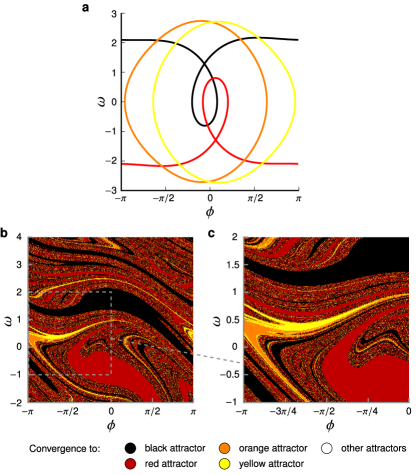
Figure 1: (Color online) Damped pendulum with fractal basin boundaries. Damped pendulum with fractal basin boundaries. (a) Attractors of the damped pendulum with time-dependent forcing from Eqn. (3). (b) State space of the pendulum at $t=0$. Black/red/orange/yellow colouring indicates convergence to the black/red/orange/yellow attractor. Convergence to other attractors is indicated by white colouring. (c) Detail of dashed square from (b).

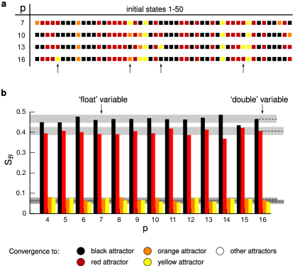
Figure 2: (Color online) Basin stability in the pendulum with fractal basin boundaries. (a) Numerical integrations for a fixed set of fifty initial states at different values of the numerical precision $p$. The squares in each column correspond to the same initial state, and their respective colours indicate which state the system converges to from there at given precision $p$. Black/red/orange/yellow colouring indicates convergence to the black/red/orange/yellow attractor. (b) Estimated basin stability $\hat{S}_{\mathcal{B}}$ of the four attractors at different levels of $p$ using $N=1000$. The basin stability of the black/red/orange/yellow attractor is shown by the height of the black/red/orange/yellow bar. The grey shadows indicate the standard error of $\hat{S}_{\mathcal{B}}(p=16)$ .

So let us first investigate how fractal basin boundaries impact the accuracy of $\hat{S}_{\mathcal{B}}$ by studying the Wada pendulum (Battelino et al., 1988; Grebogi et al., 1988). Consider a damped, driven pendulum that is subject to a time-dependent forcing:

$$\dot{\phi}=\omega,\hskip 8.5359pt\dot{\omega}=X\cos t-\alpha\omega-K\sin\phi\;.$$ (3)

For $\alpha=0.1$, $K=1$ and $X=7/4$, this system has several attractors (Kennedy and Yorke, 1991). The four dominant of them, all limit cycles with period $2\pi$, are shown in Fig. 1a: The black and red attractors correspond to rotations of the pendulum, and the orange and yellow attractors are librations. Their respective basins of attraction at $t=0$ are shown in Fig. 1b. Certain regions in this figure appear sprinkled with dots belonging to the different basins, i.e. the boundary between the basins is not easily discernible and remains so when zooming in (Fig. 1c). It is a fractal, resulting from the so-called Wada property of the basins.

Three (or more) subsets of a space are said to have the Wada property if any point on the boundary of one subset is also on the boundary of the two others (Kennedy and Yorke, 1991; Nusse and Yorke, 1996). For the pendulum, the black basin, the red basin and the union of the orange and yellow basins have the Wada property (Kennedy and Yorke, 1991; Nusse and Yorke, 1996). This means that starting within the rounding error $\varepsilon$ of the boundary, a trajectory could in principle converge to any of the four attractors.

To verify this empirically, we write $\varepsilon=10^{-p}$ with $p$ denoting precision, and discard all information after the $p$-th significant decimal digit in the floating point variables used in all individual operations of the numerical integration. We use 64 bit double precision to allow for a maximum of $p=16$, while using untruncated 32 bit single precision would correspond to $p\approx 7$. For different values of $p$, we integrate a fixed set of 50 initial states $x(0)$, drawn uniformly at random from the rectangle ${R}=[-\pi,\pi]\times[-2,4]$.

Fig. 2a, reveals that some initial states, particularly those indicated by arrows, indeed lead to different outcomes for different values of $p$. To investigate how $\hat{S}_{\mathcal{B}}$ depends on $p$, we let $\mu$ be the uniform distribution on ${R}$ yielding a sample of $N=1,000$ random initial states which are integrated with different precisions $p$, leading to estimates $\hat{S}_{\mathcal{B}}(p)$. As depicted in Fig. 2b, there seems to be no systematic influence of $p$ on $\hat{S}_{\mathcal{B}}(p)$. Indeed, most of the individual values of $\hat{S}_{\mathcal{B}}(p)$ are within one standard error of the most precise value $\hat{S}_{\mathcal{B}}(16)$. This suggests that, in contrast to long-term prediction for individual initial states (cf. Fig. 2a), $\hat{S}_{\mathcal{B}}$ is robust under variation of $p$.

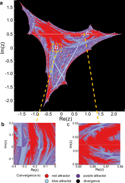
Figure 3: (Color online) Intermingled basins of the quadratic map. (a) Phase space portrait of the three attractors (red/blue/purple line segments) of the map (Eqn. 4) with their intermingled basins of attraction coloured alike. The black area corresponds to initial conditions for which the dynamics diverge. Below are zoom-ins of two regions, (b)and (c). The locations of the attractors (line segments, see (Alexander et al., 1992)) are highlighted by red/blue/purple bars (not in scale).

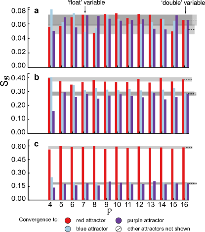
Figure 4: (Color online) Basin stability estimation for the quadratic map. (a) $\hat{S}_{\mathcal{B}}$ of the the red/blue/purple attractors at different levels of $p$, using ${R}=[-1.8,2.4]\times[-2.4,1.8]$. (b) $\hat{S}_{\mathcal{B}}$ with ${R}$ corresponding to Fig. 3 inset (1), (c) $\hat{S}_{\mathcal{B}}$ with ${R}$ corresponding to Fig. 3 inset (2). The basin stability is shown by the height of the red/blue/purple bar, the grey shadows indicate the standard error of $\hat{S}_{\mathcal{B}}(16)$.

Another extreme case are attractors whose basins are not open as for most systems (Milnor, 1985) but rather have an empty interior. The complement of such a riddled basin intersects every disk in a set of positive measure (Alexander et al., 1992; Ott et al., 1994; Lai and Grebogi, 1996; Lai et al., 1996). This means that all points in its basin of attraction have pieces of another attractor basin arbitrarily closely nearby (Ott et al., 1994).

Physical systems exhibiting riddled basins are the damped, periodically-driven particle moving in a special potential (Sommerer and Ott, 1993) or coupled time-delayed systems (Ashwin and Timme, 2005; Chaudhuri and Prasad, 2014; Jiang, 2000). There are also experimental observations for laser-cooled ions in a Paul trap (Shen et al., 2008) indicating a riddled phase space structure.

In the following, we investigate the impact of riddled basins of attraction on $\hat{S}_{\mathcal{B}}$ using a conceptual example (Alexander et al., 1992; Lopes, 1992), i.e. the following quadratic map on the complex plane:

$$F_{\lambda}(z)=z^{2}-(1+\lambda i)\bar{z},\hskip 8.5359pt\lambda=1.02871376822\,.$$ (4)

This map has three different attractors on the complex plane which are shown in Fig. 3; for simplicity they are referred to as the red/blue/purple attractors with their respective basin of attraction in the following. Interestingly, the three basins of attraction are not just riddled, they are intermingled. A basin of attraction is called intermingled if any open set which intersects one basin in a set of positive measure also intersects each of the other basins in a set of positive measure (Kan, 1994; Lai and Grebogi, 1995).

The fact that there is a positive probability to end up in a different attractor around each initial condition inside a riddled/intermingled basin of attraction renders these systems effectively non-deterministic (Sommerer and Ott, 1993). As in the case of Wada boundaries, slight variations of initial conditions or numerical imprecisions will affect any forecast of the system’s long-term behaviour.

Again, we investigate the effect of limited numerical precision on the significance of $\hat{S}_{\mathcal{B}}$. In Fig. 4a we depict the result of estimating $S_{\mathcal{B}}$ for varying $p$ using ${R}=[-1.8,2.4]\times[-2.4,1.8]$, i.e. the region pictured in Fig. 3a. We observe a large variation of $\hat{S}_{\mathcal{B}}$ of up to $50\%$ compared to the most precise estimation $\hat{S}_{\mathcal{B}}(16)$ and no systematic dependence on $p$.

In Fig. 3c we zoomed into the neighbourhood of the red attractor, where the share of the corresponding red basin is increasing in proximity of the attractor. In particular, the measure of this basin of attraction, restricted to an $\epsilon$-neighbourhood of the attractor, approaches unit probability for $\epsilon\to 0$ (Alexander et al., 1992). This apparent behaviour provides an explanation for Fig. 4c where we determined $\hat{S}_{\mathcal{B}}(p)$ for Fig. 3c. In contrast to our previous observation, the fluctuations of $\hat{S}_{\mathcal{B}}(p)$ almost stay within one standard error and the estimation appears to be more robust. For reference, Fig. 4b depicts $\hat{S}_{\mathcal{B}}(p)$ for Fig. 3b not containing any (part of) an attractor. On the one hand, the variation of $\hat{S}_{\mathcal{B}}(p)$ exceeds one standard error, up to about $20\%$ compared to $\hat{S}_{\mathcal{B}}(16)$, such that our estimation is more sensitive to numerical imprecisions than in Fig. 4b; on the other hand the variations are smaller than in our first experiment.

In conclusion, we applied the Monte-Carlo estimation procedure of basin stability in two cases, i.e. basins with fractal boundaries and riddled/intermingled basins of attraction. In the former case, we find that while the asymptotic properties of individual trajectories still cannot be determined robustly, the converse is true for the basin stability estimation. It remains an open question for future research, how exactly (in a quantitative sense) the numerical estimation uncertainty might be derived from the actual basin geometry. In the latter case, however, we find that the results can vary drastically with the chosen precision. The effect of rounding errors is comparable or even larger than the standard error of the sampling. Only if the sample region ${R}$ is chosen in some sense ”close enough” to the actual attractor of interest, the foliated structure of the surrounding basins allows for a meaningful numerical estimation.

What are practical implications for the application of basin stability? In general, it is sufficient if the rounding error of an estimation is smaller than its sampling error to get a significant result. However, any numerical procedure is subject to a finite numerical precision and we have to assume that in practice it will not be high enough to reach this goal in dynamical systems with intricate basin geometries. If there is no prior knowledge available, a good starting point is to actually visualize the interesting part of the phase space to get a first idea of the appearance of, e.g., fractal sets. If any are detected, it is necessary to use the highest available numerical precision $p_{h}$ to get $\hat{S}_{\mathcal{B}}(p_{h})$, potentially avoiding artifacts respectively insignificant estimations. We suggest to repeat the $S_{\mathcal{B}}$ estimation at a lower numerical precision $p_{l}$ and take the difference $\hat{e}_{p}=|\hat{S}_{\mathcal{B}}(p_{h})-\hat{S}_{\mathcal{B}}(p_{l})|$ as a straight-forward (rough) estimator of the variability of $\hat{S}_{\mathcal{B}}(p)$ with $p$ and, by way of extrapolation, as a rough estimate of the remaining standard error of $\hat{S}_{\mathcal{B}}(p_{h})$ as an estimate of $S_{\mathcal{B}}$ due to finite numerical precision. To assess the influence of rounding errors on $\hat{S}_{\mathcal{B}}$ then compare $\hat{e}_{p}$ with the standard error of $\hat{S}_{\mathcal{B}}(p_{h})$ as an estimate of $S_{\mathcal{B}}(p_{h})$ due to sampling, which can be estimated as $\hat{s}_{p}=\sqrt{\hat{S}_{\mathcal{B}}(p_{h})(1-\hat{S}_{\mathcal{B}}(p_{h}))/N}$. If $\hat{e}_{p}<\hat{s}_{p}$, rounding has no significant effect on the estimation quality. For instance, this could be implemented by comparing the results at double and single precision computations.

The authors gratefully acknowledge the support of BMBF, CoNDyNet, FK. 03SF0472A.

References

- Pisarchik and Feudel (2014) A. N. Pisarchik and U. Feudel, Physics Reports 540, 167 (2014).
- Lyapunov (1907) A. M. Lyapunov, Annales de la Faculté des sciences de Toulouse: Mathématiques 2, 203 (1907).
- Hahn (1958) W. Hahn, Mathematische Annalen 136, 430 (1958).
- Malisoff and Mazenc (2009) M. Malisoff and F. Mazenc, Constructions of Strict Lyapunov Functions, 1st ed., Communications and Control Engineering (Springer London, London, 2009) pp. XVI, 386.
- Giesl et al. (2016) P. Giesl, B. Hamzi, M. Rasmussen, and K. N. Webster, arXiv preprint (2016), arXiv:1601.01568 .
- Menck et al. (2013) P. J. Menck, J. Heitzig, N. Marwan, and J. Kurths, Nature Physics 9, 89 (2013).
- Menck et al. (2014) P. J. Menck, J. Heitzig, J. Kurths, and Hans-Joachim Schellnhuber, Nature Communications 5, 3969 (2014).
- Rodrigues et al. (2016) F. A. Rodrigues, T. K. D. Peron, P. Ji, and J. Kurths, Physics Reports 610, 1 (2016).
- Kim et al. (2015) H. Kim, S. H. Lee, and P. Holme, New Journal of Physics 17, 113005 (2015).
- Kim et al. (2016) H. Kim, S. H. Lee, and P. Holme, arXiv preprint (2016), arXiv:1602.01712 .
- Schmietendorf et al. (2014) K. Schmietendorf, J. Peinke, R. Friedrich, and O. Kamps, The European Physical Journal: Special Topics , 1 (2014).
- Martens et al. (2016) E. A. Martens, M. J. Panaggio, and D. M. Abrams, New Journal of Physics 18, 022002 (2016).
- Zou et al. (2014) Y. Zou, T. Pereira, M. Small, Z. Liu, and J. Kurths, Physical Review Letters 112, 114102 (2014).
- Leng et al. (2016) S. Leng, W. Lin, and J. Kurths, Scientific Reports 6, 21449 (2016).
- Mitra et al. (2015) C. Mitra, J. Kurths, and R. V. Donner, Scientific Reports 5, 16196 (2015).
- Nusse and Yorke (1996) H. E. Nusse and J. A. Yorke, Physica D: Nonlinear Phenomena 90, 242 (1996).
- Milnor (1985) J. Milnor, Communications in Mathematical Physics 99, 177 (1985).
- Evans and Swartz (2000) M. Evans and T. Swartz, Approximating Integrals via Monte Carlo and Deterministic Methods (OUP Oxford, 2000).
- von Neumann (1951) J. von Neumann, J. Res. Nat. Bur. Stand. 12, 36 (1951).
- Grebogi et al. (1983a) C. Grebogi, E. Ott, and J. A. Yorke, Physical Review Letters 50, 935 (1983a).
- McDonald et al. (1985) S. W. McDonald, C. Grebogi, E. Ott, and J. A. Yorke, Physica 17D , 125 (1985).
- Grebogi et al. (1983b) C. Grebogi, S. W. McDonald, E. Ott, and J. A. Yorke, Physics Letters 99A, 415 (1983b).
- Grebogi et al. (1987) C. Grebogi, E. Ott, and J. A. Yorke, Science (New York, N.Y.) 238, 632 (1987).
- Lorenz (1963) E. N. Lorenz, Journal of the Atmospheric Sciences 20, 130 (1963).
- Bergé and Dubois (1983) P. Bergé and M. Dubois, Physics Letters A 93, 365 (1983).
- Battelino et al. (1988) P. M. Battelino, C. Grebogi, E. Ott, J. A. Yorke, and E. D. Yorke, Physica D: Nonlinear Phenomena 32, 296 (1988).
- Grebogi et al. (1988) C. Grebogi, H. E. Nusse, E. Ott, and J. A. Yorke, in Dynamical Systems. Proceeding of the Special Year held at the University of Maryland, College Park, 1986-87, Vol. 1342 (1988) pp. 220–250.
- Kennedy and Yorke (1991) J. Kennedy and J. A. Yorke, Physica D: Nonlinear Phenomena 51, 213 (1991).
- Alexander et al. (1992) J. Alexander, J. A. Yorke, Z. You, and I. Kan, International Journal of Bifurcation and Chaos 02, 795 (1992).
- Ott et al. (1994) E. Ott, J. Alexander, I. Kan, J. Sommerer, and J. Yorke, Physica D: Nonlinear Phenomena 76, 384 (1994).
- Lai and Grebogi (1996) Y.-C. Lai and C. Grebogi, Phys. Rev. E 53, 1371 (1996).
- Lai et al. (1996) Y.-C. Lai, C. Grebogi, J. Yorke, and S. Venkataramani, Physical Review Letters 77, 55 (1996).
- Sommerer and Ott (1993) J. C. Sommerer and E. Ott, Nature 365, 138 (1993).
- Ashwin and Timme (2005) P. Ashwin and M. Timme, Nonlinearity 18, 29 (2005).
- Chaudhuri and Prasad (2014) U. Chaudhuri and A. Prasad, Physics Letters A 378, 713 (2014).
- Jiang (2000) Y. Jiang, Physics Letters A 267, 342 (2000).
- Shen et al. (2008) J.-l. Shen, H.-w. Yin, J.-h. Dai, and H.-j. Zhang, Chinese Physics Letters 13, 81 (2008).
- Lopes (1992) A. O. Lopes, Comput. & Graphics 16, 15 (1992).
- Kan (1994) I. Kan, Bulletin of the American Mathematical Society 31, 68 (1994).
- Lai and Grebogi (1995) Y. C. Lai and C. Grebogi, Physical Review E 52 (1995).