Singular Infinite Horizon Quadratic Control of Linear Systems with Known Disturbances:
A Regularization Approach

Abstract

An optimal control problem with an infinite horizon quadratic cost functional for a linear system with a known additive disturbance is considered. The feature of this problem is that a weight matrix of the control cost in the cost functional is singular. Due to this singularity, the problem can be solved neither by application of the Pontriagin’s Maximum Principle, nor using the Hamilton-Jacobi-Bellman equation approach, i.e. this problem is singular. Since the weight matrix of the control cost, being singular, is not in general zero, only a part of the control coordinates is singular, while the others are regular. This problem is solved by a regularization method. Namely, it is associated with a new optimal control problem for the same equation of dynamics. The cost functional in this new problem is the sum of the original cost functional and an infinite horizon integral of the squares of the singular control coordinates with a small positive weight. Due to a smallness of this coefficient, the new problem is a partial cheap control problem. Using a perturbation technique, an asymptotic analysis of this partial cheap control problem is carried out. Based on this analysis, the infimum of the cost functional in the original problem is derived, and a minimizing sequence of state-feedback controls is designed. An illustrative example of a singular trajectory tracking is presented.

1 Introduction

In this paper, an optimal control of a linear differential equation with constant coefficients for the state and the control, and with a known additive disturbance is considered. The control process is evaluated by an infinite horizon quadratic cost functional to be minimized by a proper choice of the control. A weight matrix of the control cost in this cost functional is singular, meaning that the optimal control problem is singular. Namely, the considered problem can be solved neither by application of the Pontriagin’s Maximum Principle [1], nor using the Hamilton-Jacobi-Bellman equation approach (Dynamic Programming approach) [2]. This occurs because the problem of maximization of the corresponding variational Hamiltonian with respect to the control either has no solution, or has infinitely many solutions. To the best of our knowledge, five main methods of solution of singular optimal control problems can be distinguished in the literature. Thus, higher order necessary or sufficient optimality conditions can be helpful in solving a singular optimal control problem (see e.g. [3, 4, 5, 6, 7, 8] and references therein). However, such conditions fail to yield a candidate optimal control (an optimal control) for the problem, having no solution (an optimal control) in the class of regular functions, even if the cost functional has a finite infimum in this class of functions. The second method propose to derive a singular optimal control as a minimizing sequence of regular open-loop controls, i.e., a sequence of regular control functions of time, along which the cost functional tends to its infimum (see e.g. [7, 9, 10] and references therein). The derivation of the minimizing sequence is based on the Krotov’s sufficient optimality conditions [7] and theory of linear first order partial differential equations. A generalization of this method is the extension approach [11, 12, 13]. The third method combines geometric and analytic approaches. Namely, this method is based on a decomposition of the state space into ”regular” and ”singular” subspaces, and a design an optimal open loop control as a sum of impulsive and regular functions (see e.g. [14, 15, 16, 17] and references therein). The fourth method consists in searching a solution of a singular optimal control problem in a properly defined class of generalized functions (see e.g. [18]). Finally, the fifth method based on a regularization of the original singular problem by a ”small” correction of its ”singular” cost functional (see e.g. [19, 20, 21] and references therein). Such a regularization is a kind of the Tikhonov’s regularization of ill-posed problems [22]. This method yields the solution of the original problem in the form of a minimizing sequence of state-feedback controls.

In the present paper, a singular infinite horizon linear-quadratic optimal control problem with a known additive time-varying disturbance in the dynamics is considered. To the best of our knowledge, such a problem has not yet been considered in the literature. This problem is treated by the regularization, which yields an auxiliary partial cheap control problem. Using perturbation techniques, an asymptotic behavior of the solution to the auxiliary control problem is analyzed. Based on this analysis, the existence of the finite infimum of the cost functional in the original (singular) control problem is established. The expression for this infimum is derived. The minimizing sequence of state-feedback controls in the original problem also is designed. The theoretical results are applied to solution of a singular tracking problem.

The paper is organized as follows. In Section 2, the rigorous formulation of the problem is presented. Objectives of the paper are stated. In Section 3, a regularization of the original singular optimal control problem is made, yielding a partial cheap control problem. An asymptotic analysis of this problem is carried out in Section 4. The solution of the original singular optimal control problem is derived in Section 5. Section 6 deals with an illustrative example. Section 7 contains some concluding remarks. Proofs of some technical lemmas and of one of the main theorems are placed in Appendices.

2 Problem Statement

2.1 Initial control problem and main assumptions

Consider the following controlled differential equation:

$$\frac{dZ(t)}{dt}={\mathcal{A}}Z(t)+{\mathcal{B}}U(t)+{\mathcal{F}}(t),\ \ \ t\geq 0,\ \ \ Z(0)=Z_{0},$$ (1)

where $Z(t)\in E^{n}$ is the state vector; $U(t)\in E^{r}$, ($r\leq n$) is the control; ${\mathcal{A}}$ and ${\mathcal{B}}$ are given constant matrices of corresponding dimensions; ${\mathcal{F}}(t)$, $t\geq 0$ is a given vector-valued function; $Z_{0}\in E^{n}$ is a given vector; for any integer $m>0$, $E^{m}$ denotes the real Euclidean space of the dimension $m$.

The cost functional, to be minimized by $U$, is

$${\mathcal{J}}\big{(}U\big{)}\overset{\triangle}{=}\int\limits_{0}^{+\infty}\left[Z^{T}(t){\mathcal{D}}Z(t)+U^{T}(t)GU(t)\right]dt,$$ (2)

where ${\mathcal{D}}$ is a given constant symmetric matrix of corresponding dimension; the given constant $r\times r$-matrix $G$ has the form

$$G=\mathrm{diag}\big{(}g_{1},...,g_{q},\underbrace{0,...,0}_{r-q}\big{)},\ \ \ \ 0\leq q<r,$$ (3)

the superscript $"T"$ denotes the transposition.

In what follows, we assume:

(A1) The matrix ${\mathcal{B}}$ has full rank $r$;

(A2) the matrix ${\mathcal{D}}$ is positive semi-definite (${\mathcal{D}}\geq 0$);

(A3) $g_{k}>0$, $k=1,...,q$;

(A4) the function ${\mathcal{F}}(t)$ satisfies the inequality $\|{\mathcal{F}}(t)\|\leq a\exp(-\gamma t)$, $t\geq 0$, where $a>0$ and $\gamma>0$ are some constants.

Since the matrix $G$ is singular, the optimal control problem (1)-(2) is singular.

Consider the set ${\mathcal{P}}$ of all functions $p(w,t):E^{n}\times\left[0,+\infty\right)\rightarrow E^{r}$, which are measurable w.r.t. $t\geq 0$ for any fixed $w\in E^{n}$ and satisfy the local Lipschitz condition w.r.t. $w\in E^{n}$ uniformly in $t\geq 0$.

Definition 1

Let $U(Z,t)$, $(Z,t)\in E^{n}\times\left[0,+\infty\right)$, be a function belonging to the set ${\mathcal{P}}$. The function $U(Z,t)$ is called an admissible state-feedback control in the problem (1)-(2) if the following conditions hold: (a) the initial-value problem (1) for $U(t)=U(Z,t)$ has the unique locally absolutely continuous solution $Z(t)$ on the entire interval $\left[0,+\infty\right)$; (b) $Z(t)\in L^{2}\left[0,+\infty;E^{n}\right]$; (c) $U\big{(}Z(t),t\big{)}\in L^{2}\left[0,+\infty;E^{r}\right]$. The set of all such $U(Z,t)$ is denoted by ${\mathcal{M}}_{U}$.

Denote

$$\mathcal{J}^{*}\overset{\triangle}{=}\inf_{U(Z,t)\in\mathcal{M}_{U}}\mathcal{J}\big{(}U(Z,t)\big{)}.$$ (4)

Remark 2

Since ${\mathcal{D}}\geq 0$ and $G\geq 0$, then the infimum (4) is nonnegative. Moreover, if ${\mathcal{M}}_{U}\neq\emptyset$, this infimum is finite.

Definition 3

The control sequence $\big{\{}U_{k}(Z,t)\big{\}}$, $U_{k}(Z,t)\in\mathcal{M}_{U}$, $(k=1,2,...)$, is called minimizing in the problem (1)-(2) if

$$\lim_{k\rightarrow+\infty}\mathcal{J}\big{(}U_{k}(Z,t)\big{)}=\mathcal{J}^{*}.$$ (5)

If there exists $U^{\ast}(Z,t)\in\mathcal{M}_{U}$, for which

$$\mathcal{J}\big{(}U^{\ast}(Z,t)\big{)}=\mathcal{J}^{*},$$ (6)

this control is called optimal in the problem (1)-(2). In this case there exists a minimizing control sequence, point-wise convergent to $U^{\ast}(Z,t)$ for a. a. $(Z,t)\in E^{n}\times\left[0,+\infty\right)$.

2.2 Transformation of the problem (1)-(2)

Let us partition the matrix ${\mathcal{B}}$ into blocks as ${\mathcal{B}}=\Big{(}{\mathcal{B}}_{1},{\mathcal{B}}_{2}\Big{)}$, where the blocks ${\mathcal{B}}_{1}$ and ${\mathcal{B}}_{2}$ are of dimensions $n\times q$ and $n\times(r-q)$, respectively.

We assumed that:

(A5)  $\det\left({\mathcal{B}}_{2}^{T}{\mathcal{DB}}_{2}\right)\neq 0$.

By ${\mathcal{B}}_{c}$, we denote a complement matrix to the matrix ${\mathcal{B}}$, i.e., the matrix of dimension $n\times(n-r)$, and such that the block matrix $({\mathcal{B}}_{c},{\mathcal{B}})$ is nonsingular. Hence, the block matrix $\widetilde{{\mathcal{B}}}_{c}=\left({\mathcal{B}}_{c},{\mathcal{B}}_{1}\right)$ is a complement matrix to ${\mathcal{B}}_{2}$.

Consider the following matrices:

$${\mathcal{H}}=({\mathcal{B}}_{2}^{T}{\mathcal{D}}{\mathcal{B}}_{2})^{-1}{\mathcal{B}}_{2}^{T}{\mathcal{D}}\widetilde{{\mathcal{B}}}_{c},\ \ \ \ {\mathcal{L}}=\widetilde{{\mathcal{B}}}_{c}-{\mathcal{B}}_{2}{\mathcal{H}}.$$ (7)

Now, using the block matrix $\left({\mathcal{L}},{\mathcal{B}}_{2}\right)$, we transform the state in the control problem (1)-(2) as follows:

$$Z(t)=\left({\mathcal{L}},{\mathcal{B}}_{2}\right)z(t),$$ (8)

where $z(t)\in E^{n}$ is a new state.

By virtue of the results of [23], the transformation (8) is nonsingular.

Remark 4

In what follows, we use the notation $O_{n_{1}\times n_{2}}$ for the zero matrix of dimension $n_{1}\times n_{2}$, excepting the cases where the dimension of zero matrix is obvious. In such cases, we use the notation $0$ for the zero matrix. By $I_{m}$, we denote the identity matrix of dimension $m$.

Based on the results of [24] (Lemma 1), we have the following lemma.

Lemma 5

Let the assumptions (A1), (A2), (A4), (A5) be valid. Then, transforming the state variable of the problem (1)-(2) in accordance with (8), and redenoting the control as $u(t)$, we obtain the control problem with the dynamics

$$\frac{dz(t)}{dt}=Az(t)+Bu(t)+f(t),\ \ \ \ z(0)=z_{0},\ \ \ t\geq 0,$$ (9)

and the cost functional

$$J(u)=\int\limits_{0}^{+\infty}\left[z^{T}(t)Dz(t)+u^{T}(t)Gu(t)\right]dt,$$ (10)

where

$$A=\left({\mathcal{L}},{\mathcal{B}}_{2}\right)^{-1}{\mathcal{A}}\left({\mathcal{L}},{\mathcal{B}}_{2}\right),$$ (11)

$$B=\left({\mathcal{L}},{\mathcal{B}}_{2}\right)^{-1}{\mathcal{B}}=\left(\begin{array}[]{l}B_{1}\\ B_{2}\end{array}\right),$$ (12)

$$B_{1}=\left(\begin{array}[]{c}O_{\left(n-r\right)\times r}\\ \widetilde{I}_{1}\end{array}\right),\ \ \ \ \widetilde{I}_{1}=\left(\begin{array}[]{cc}I_{q}\ ,\ O_{q\times\left(r-q\right)}&\end{array}\right),$$ (13)

$$B_{2}={\mathcal{H}}B_{1}+\widetilde{I}_{2},\ \ \ \ \widetilde{I}_{2}=\left(\begin{array}[]{cc}O_{\left(r-q\right)\times q}\ ,\ I_{r-q}&\end{array}\right),$$ (14)

$$\begin{array}[]{ll}D=\left({\mathcal{L}},{\mathcal{B}}_{2}\right)^{T}{\mathcal{D}}\left({\mathcal{L}},{\mathcal{B}}_{2}\right)=\left(\begin{array}[]{l}D_{1}\ \ \ \ \ \ \ \ \ \ \ \ \ \ \ \ \ \ \ O_{(n-r+q)\times(r-q)}\\ O_{(r-q)\times(n-r+q)}\ \ \ D_{2}\end{array}\right),&\\ &\\ D_{1}\ ={\mathcal{L}}^{T}{\mathcal{DL}},\ \ \ \ D_{2}={\mathcal{B}}_{2}^{T}{\mathcal{DB}}_{2},&\end{array}$$ (15)

$$f(t)=\left({\mathcal{L}},{\mathcal{B}}_{2}\right)^{-1}\mathcal{F}(t),$$ (16)

$$z_{0}=\left({\mathcal{L}},{\mathcal{B}}_{2}\right)^{-1}Z_{0},$$ (17)

the matrices $D_{1}$ and $D_{2}$ are symmetric, and $D_{1}$ is positive semi-definite ($D_{1}\geq 0$), $D_{2}$ is positive definite ($D_{2}>0$). Moreover, the function $f(t)$ satisfies the inequality

$$\|f(t)\|\leq a\exp(-\gamma t),\ \ \ \ t\geq 0,$$ (18)

where $a>0$ is some constant.

Remark 6

In the optimal control problem (9)-(10), the cost functional $J(u)$ is minimized by the control $u(t)$. Since the weight matrix of the control cost in the cost functional $J(u)$ is singular, the solution (if any) of this game can be obtained neither by the Pontriagin’s Maximum Principle nor by the Hamilton-Jacobi-Bellman equation method, meaning that the problem (9)-(10) is singular. The set $M_{u}$ of admissible state-feedback controls $u(z,t)$ in the problem (9)-(10) is defined similarly to such a set $\mathcal{M}_{U}$ in the problem (1)-(2). The infimum

$$J^{*}\overset{\triangle}{=}\inf_{u(z,t)\in M_{u}}J\big{(}u(z,t)\big{)}$$ (19)

is nonnegative. Moreover, if ${M}_{u}\neq\emptyset$, this infimum is finite. The minimizing control sequence $\{u_{k}(z,t)\}$ and the optimal state-feedback control $u^{*}(z,t)$ in this problem are defined similarly to those in the problem (1)-(2), (see (5) and (6), respectively).

2.3 Equivalence of the problems (1)-(2) and (9)-(10)

Lemma 7

Let the assumptions (A1), (A2), (A5) be valid. Then, the sets $M_{u}$ and ${\mathcal{M}}_{U}$ of the admissible state-feedback controls in the problems (9)-(10) and (1)-(2), respectively, are either both nonempty or both empty.

Proof. The statement of the lemma directly follows from Lemma 5, the invertibility of the transformation (8), and the definitions of the sets $\mathcal{M}_{U}$ and $M_{u}$.   

Lemma 8

Let the assumptions (A1), (A2), (A5) be valid. Let $M_{u}\neq\emptyset$. Then, the infimum values $J^{*}$ and $\mathcal{J}^{*}$ of the cost functionals in the problems (9)-(10) and (1)-(2), respectively, are finite and equal to each other.

Proof. The finiteness of $J^{*}$ and $\mathcal{J}^{*}$ follows immediately from the condition $M_{u}\neq\emptyset$, Lemma 7, and Remarks 2 and 6.

Proceed to the proof of the equality

$$J^{*}=\mathcal{J}^{*}.$$ (20)

Due to the definition of $J^{*}$, there exists a control sequence $\{u_{k}(z,t)\}$, $u_{k}(z,t)\in M_{u}$, $(k=1,2,...)$, such that

$$\lim_{k\rightarrow+\infty}J\big{(}u_{k}(z,t)\big{)}=J^{*}.$$ (21)

Similarly, due to the definition of $\mathcal{J}^{*}$, there exists a control sequence $\{\widehat{U}_{k}(Z,t)\}$, $\widehat{U}_{k}(Z,t)\in\mathcal{M}_{U}$, $(k=1,2,...)$, such that

$$\lim_{k\rightarrow+\infty}\mathcal{J}\big{(}\widehat{U}_{k}(Z,t)\big{)}=\mathcal{J}^{*}.$$ (22)

Let us define the controls

$$U_{k}(Z,t)\overset{\triangle}{=}u_{k}\big{(}(\mathcal{L},\mathcal{B}_{2})^{-1}Z,t\big{)},\ \ \ \ \hat{u}_{k}(z,t)\overset{\triangle}{=}\widehat{U}_{k}\big{(}(\mathcal{L},\mathcal{B}_{2})z,t\big{)},\ \ \ k=1,2,...\ .$$ (23)

Using Lemma 5, the invertibility of the transformation (8) and the definitions of the sets $\mathcal{M}_{U}$ and $M_{u}$, one directly obtains that

$$U_{k}(Z,t)\in\mathcal{M}_{U},\ \ \ \ \hat{u}_{k}(z,t)\in M_{u},\ \ \ k=1,2,...\ ,$$ (24)

and

$$\mathcal{J}\big{(}U_{k}(Z,t)\big{)}=J\big{(}u_{k}(z,t)\big{)},\ \ \ \ J\big{(}\hat{u}_{k}(z,t)\big{)}=\mathcal{J}\big{(}\widehat{U}_{k}(Z,t)\big{)},\ \ \ k=1,2,...\ .$$ (25)

The equations (21)-(22) and (25), as well as the facts that ${\mathcal{J}}^{\ast}$ is the infimum of the cost functional in the problem (1)-(2) and $J^{\ast}$ is the infimum of the cost functional in the problem (9)-(10), imply the inequalities

$$\mathcal{J}^{\ast}\leq J^{\ast},\ \ \ \ J^{\ast}\leq\mathcal{J}^{\ast},$$ (26)

which yield the equality (20). Thus, the lemma is proven.   

In the sequel of this paper, we deal with the optimal control problem (9)-(10). We call this problem the Original Optimal Control Problem (OOCP). As it was mentioned above, the OOCP is singular. Moreover, this problem does not have, in general, an optimal control among regular functions.

2.4 Objectives of the paper

The objectives of this paper are:
(I) to establish finiteness of the infimum of the cost functional in the OOCP;
(II) to derive an expression for this infimum;
(III) to design a minimizing sequence of state-feedback controls in the OOCP.

3 Regularization of the OOCP

3.1 Partial cheap control problem

Consider the optimal control problem with the dynamics (9) and the performance index

$$J_{\varepsilon}(u)\overset{\triangle}{=}\int\limits_{0}^{+\infty}\left[z^{T}(t)Dz(t)+u^{T}(t)(G+\mathcal{E})u(t)\right]dt\rightarrow\min_{u},$$ (27)

where

$${\mathcal{E}}=\mathrm{diag}\Big{(}\underbrace{0,...,0}_{q},\underbrace{\varepsilon^{2},...,\varepsilon^{2}}_{r-q}\Big{)},$$ (28)

and $\varepsilon>0$ is a small parameter.

Remark 9

Since the parameter $\varepsilon>0$ is small, the problem (9), (27) is a partial cheap control problem, i.e., an optimal control problem where a cost of some control coordinates in the cost functional is much smaller than costs of the state and the other control coordinates. In what follows, we call this problem the Partial Cheap Control Problem (PCCP). The case of the completely cheap control was widely studied in the literature for various control problems (see e.g. [21, 25, 26, 27, 28, 29, 30] and references therein). However, to the best of the authors’ knowledge, the partial cheap control case was analyzed only in two works. Namely, in [31] a two-time-scale decomposition of the time-invariant regulator problem with partial cheap control was carried out, yielding a near-optimal composite control. In [24], a finite-horizon zero-sum linear-quadratic differential game with partial cheap control of the minimizing player was studied.

3.2 Optimal state-feedback control of the PCCP

We look for such a control in the same set of the admissible controls as was introduced earlier for the OOCP, i.e., in the set $M_{u}$.

Consider the algebraic matrix Riccati equation

$$PA+A^{T}P-PS(\varepsilon)P+D=0,\$$ (29)

where

$$S(\varepsilon)=B(G+\mathcal{E})^{-1}B^{T}.$$ (30)

By virtue of the inequality (18) and the results of [32], if for a given $\varepsilon>0$ the equation (29) has a symmetric solution $P^{*}(\varepsilon)\geq 0$ such that the matrix

$$\mathcal{A}(\varepsilon)\overset{\triangle}{=}A-S(\varepsilon)P^{*}(\varepsilon)$$ (31)

is a Hurwitz one, then the optimal control of the PCCP exists in the set of the admissible state-feedback controls $M_{u}$. This control is unique and it has the form

$$u^{*}_{\varepsilon}(z,t)=-(G+\mathcal{E})^{-1}B^{T}P^{*}(\varepsilon)z-(G+\mathcal{E})^{-1}B^{T}h(t),$$ (32)

where the $n$-dimensional vector-valued function $h(t)$, $t\in[0,+\infty)$ is the unique solution of the terminal-value problem

$$\frac{dh(t)}{dt}=-\mathcal{A}^{T}(\varepsilon)h(t)-P^{*}(\varepsilon)f(t),\ \ \ \ \ h(+\infty)=0.$$ (33)

The optimal value of the cost functional in the PCCP has the form

$$J_{\varepsilon}^{*}=z_{0}^{T}P^{*}(\varepsilon)z_{0}+2h^{T}(0)z_{0}+s(0),$$ (34)

where the scalar function $s(t)$, $t\in[0,+\infty)$ is the unique solution of the terminal-value problem

$$\frac{ds(t)}{dt}=-2h^{T}(t)f(t)+h^{T}(t)S(\varepsilon)h(t),\ \ \ \ s(+\infty)=0.$$ (35)

4 Asymptotic Analysis of the PCCP

4.1 Asymptotic solution of the equation (29)

First of all, let as note that the matrix $S(\varepsilon)$, appearing in this equation, can be represented (similarly to the results of [24]) in the following block form:

$$S(\varepsilon)=\left(\begin{array}[]{lr}S_{1}&S_{2}\\ &\\ S_{2}^{T}&(1/\varepsilon^{2})S_{3}(\varepsilon)\end{array}\right),$$ (36)

where

$$S_{1}=\left(\begin{array}[]{l}O_{(n-r)\times(n-r)}\ \ O_{(n-r)\times q}\\ O_{q\times(n-r)}\ \ \ \ \ \ \ \widetilde{G}^{-1}\end{array}\right),\ \ \ S_{2}=\left(\begin{array}[]{c}O_{(n-r)\times(r-q)}\\ H_{1}\end{array}\right),$$ (41)

$$S_{3}(\varepsilon)=\varepsilon^{2}H_{2}+I_{r-q},$$ (42)

$$\widetilde{G}=\mathrm{diag}\big{(}g_{1},...,g_{q}\big{)},\ \ H_{1}=H_{3}{\mathcal{H}}^{T},\ \ H_{2}={\mathcal{H}}\left(\begin{array}[]{c}O_{(n-r)\times(r-q)}\\ H_{1}\end{array}\right),$$ (45)

$$H_{3}=\Big{(}O_{q\times(n-r)},\widetilde{G}^{-1}\Big{)},$$ (46)

${\mathcal{H}}$ is defined in (7).

Due to (36)-(46), the left-hand side of the equation (29) has a singularity at $\varepsilon=0$. To remove this singularity, we seek the symmetric solution $P(\varepsilon)$ of the equation (29) in the block form

$$P(\varepsilon)=\left(\begin{array}[]{cc}P_{1}(\varepsilon)&\varepsilon P_{2}(\varepsilon)\\ &\\ \varepsilon P_{2}^{T}(\varepsilon)&\ \varepsilon P_{3}(\varepsilon)\end{array}\right),$$ (47)

where the blocks $P_{1}(\varepsilon)$, $P_{2}(\varepsilon)$ and $P_{3}(\varepsilon)$ have the dimensions $(n-r+q)\times(n-r+q)$, $(n-r+q)\times\left(r-q\right)$ and $\left(r-q\right)\times\left(r-q\right)$, respectively; and

$$P_{1}^{T}(\varepsilon)=P_{1}(\varepsilon),\ \ \ P_{3}^{T}(\varepsilon)=P_{3}(\varepsilon).$$ (48)

We also partition the matrix $A$ into blocks as follows:

$$A=\left(\begin{array}[]{cc}A_{1}&A_{2}\\ &\\ A_{3}&A_{4}\end{array}\right),$$ (49)

where the blocks $A_{1}$, $A_{2}$, $A_{3}$ and $A_{4}$ have the dimensions $(n-r+q)\times(n-r+q)$, $(n-r+q)\times\left(r-q\right)$, $(r-q)\times(n-r+q)$ and $\left(r-q\right)\times\left(r-q\right)$, respectively.

Substitution of the block representations for the matrices $D$, $S(\varepsilon)$, $P(\varepsilon)$, and $A$ (see (15), (36), (47), and (49)) into the equation (29) yields after a routine rearrangement the following equivalent set of Riccati-type algebraic matrix equations with respect to $P_{1}(\varepsilon)$, $P_{2}(\varepsilon)$ and $P_{3}(\varepsilon)$:

$$P_{1}(\varepsilon)A_{1}+\varepsilon P_{2}(\varepsilon)A_{3}+A_{1}^{T}P_{1}(\varepsilon)+\varepsilon A_{3}^{T}P_{2}^{T}(\varepsilon)-P_{1}(\varepsilon)S_{1}P_{1}(\varepsilon)$$

$$-\varepsilon P_{2}(\varepsilon)S_{2}^{T}P_{1}(\varepsilon)-\varepsilon P_{1}(\varepsilon)S_{2}P_{2}^{T}(\varepsilon)-P_{2}(\varepsilon)S_{3}(\varepsilon)P_{2}^{T}(\varepsilon)+D_{1}=0,$$ (50)

$$P_{1}(\varepsilon)A_{2}+\varepsilon P_{2}(\varepsilon)A_{4}+\varepsilon A_{1}^{T}P_{2}(\varepsilon)+\varepsilon A_{3}^{T}P_{3}(\varepsilon)-\varepsilon P_{1}(\varepsilon)S_{1}P_{2}(\varepsilon)$$

$$-\varepsilon^{2}P_{2}(\varepsilon)S_{2}^{T}P_{2}(\varepsilon)-\varepsilon P_{1}(\varepsilon)S_{2}P_{3}(\varepsilon)-P_{2}(\varepsilon)S_{3}(\varepsilon)P_{3}(\varepsilon)=0,$$ (51)

$$\varepsilon P_{2}^{T}(\varepsilon)A_{2}+\varepsilon P_{3}(\varepsilon)A_{4}+\varepsilon A_{2}^{T}P_{2}(\varepsilon)+\varepsilon A_{4}^{T}P_{3}(\varepsilon)-\varepsilon^{2}P_{2}^{T}(\varepsilon)S_{1}P_{2}(\varepsilon)$$

$$-\varepsilon^{2}P_{3}(\varepsilon)S_{2}^{T}P_{2}(\varepsilon)-\varepsilon^{2}P_{2}^{T}(\varepsilon)S_{2}P_{3}(\varepsilon)-P_{3}(\varepsilon)S_{3}(\varepsilon)P_{3}(\varepsilon)+D_{2}=0.$$ (52)

We seek the asymptotic solution $P_{i,m}^{\mathrm{as}}(\varepsilon)$, $(i=1,2,3)$ of the system (50)-(52) in the form $P_{i,m}^{\mathrm{as}}(\varepsilon)=P_{i0}+\varepsilon P_{i1}+...+\varepsilon^{m}P_{i,m}$, where $m\geq 0$ is a given integer. In what follows, we restrict ourselves to the case of zero-order asymptotic solution, i.e., $m=0$ and

$$P_{i,0}^{\mathrm{as}}(\varepsilon)=P_{i0},\ \ \ i=1,2,3.$$ (53)

Equations for the zero-order asymptotic solution terms are obtained by substitution of (53) into (50)-(52) instead of $P_{i}(\varepsilon)$, $(i=1,2,3)$, and equating coefficients for the zero power of $\varepsilon$ on both sides of the resulting equations. Thus, we have the following system:

$$P_{10}A_{1}+A_{1}^{T}P_{10}-P_{10}S_{1}P_{10}-P_{20}P_{20}^{T}+D_{1}=0,$$ (54)

$$P_{10}A_{2}-P_{20}P_{30}=0,$$ (55)

$$\big{(}P_{30}\big{)}^{2}-D_{2}=0.$$ (56)

Solving the equations (56) and (55) with respect to $P_{30}$ and $P_{20}$, we obtain

$$P_{30}=P_{30}^{*}\overset{\triangle}{=}\big{(}D_{2}\big{)}^{1/2},\ \ \ \ P_{20}=P_{10}A_{2}\big{(}D_{2}\big{)}^{-1/2},$$ (57)

where the superscript $"1/2"$ denotes the unique symmetric positive definite square root of the corresponding symmetric positive definite matrix, while the superscript $"-1/2"$ denotes the inverse matrix for such a square root.

Since $\big{(}D_{2}\big{)}^{1/2}$ is positive definite, then there exists a positive number $\beta$ such that all eigenvalues $\lambda\Big{(}-\big{(}D_{2}\big{)}^{1/2}\Big{)}$ of the matrix $-\big{(}D_{2}\big{)}^{1/2}$ satisfy the inequality

$$\mathrm{Re}\lambda\Big{(}-\big{(}D_{2}\big{)}^{1/2}\Big{)}<-\beta.$$ (58)

Substitution of the expression for $P_{20}$ from (57) into (54) yields the algebraic matrix Riccati equation with respect to $P_{10}$

$$P_{10}A_{1}+A_{1}^{T}P_{10}-P_{10}{S}_{0}P_{10}+D_{1}=0,$$ (59)

where

$${S}_{0}=A_{2}D_{2}^{-1}A_{2}^{T}+S_{1}.$$ (60)

Based on the results of [24], we can represent the matrix $S_{0}$ in the form

$${S}_{0}=\bar{B}\Theta^{-1}\bar{B}^{T},$$ (61)

where

$$\bar{B}=\left(\begin{array}[]{l}\widetilde{B}\ ,\ A_{2}\end{array}\right),\ \ \ \ \widetilde{B}=\left(\begin{array}[]{c}O_{\left(n-r\right)\times q}\\ I_{q}\end{array}\right),$$ (62)

$$\Theta=\left(\begin{array}[]{cc}\widetilde{G}&O_{q\times\left(r-q\right)}\\ O_{\left(r-q\right)\times q}&D_{2}\end{array}\right).$$ (63)

Let $F_{1}$ be a matrix such that

$$D_{1}=F_{1}^{T}F_{1}.$$ (64)

In what follows, we assume:
(A6) The pair $(A_{1},\bar{B})$ is stabilizable;
(A7) the pair $(A_{1},F_{1})$ is detectable.

Using the equation (61), the assumptions (A6), (A7), and the results of [33], one directly obtains that the algebraic matrix Riccati equation (59) has the unique symmetric solution $P_{10}^{*}\geq 0$. Moreover, the matrix

$$\mathcal{A}_{0}\overset{\triangle}{=}A_{1}-S_{0}P_{10}^{*}$$ (65)

is a Hurwitz one. Therefore, there exists a positive number $\alpha$, ($\alpha\neq\gamma$), such that all eigenvalues $\lambda\Big{(}\mathcal{A}_{10}\Big{)}$ of this matrix satisfy the inequality

$$\mathrm{Re}\lambda\Big{(}\mathcal{A}_{0}\Big{)}<-\alpha.$$ (66)

Now, using Lemma 5 (the positive definiteness of the matrix $D_{2}$), the above mentioned features of the equation (59), and the results of [34] (Sections 3.4 and 3.6.1), we can state the following:

Lemma 10

Let the assumptions (A1)-(A3), (A5)-(A7) be valid. Then, there exists a positive number $\varepsilon_{0}$ such that for all $\varepsilon\in[0,{\varepsilon}_{0}]$ the equation (29) has the unique symmetric solution $P^{*}(\varepsilon)\geq 0$. This solution has the block form

$$P^{\ast}(\varepsilon)=\left(\begin{array}[]{cc}P_{1}^{\ast}(\varepsilon)&\varepsilon{\ P}_{2}^{\ast}(\varepsilon)\\ \varepsilon\big{(}P_{2}^{\ast}(\varepsilon)\big{)}^{T}&\varepsilon P_{3}^{\ast}(\varepsilon)\end{array}\right),$$ (67)

where the blocks $P_{1}^{\ast}(\varepsilon)$, $P_{2}^{\ast}(\varepsilon)$, $P_{3}^{\ast}(\varepsilon)$ are of dimensions $(n-r+q)\times(n-r+q)$, $(n-r+q)\times(r-q)$, $(r-q)\times(r-q)$, respectively. These blocks satisfy the inequalities

$$\|P_{i}^{\ast}(\varepsilon)-P_{i0}^{\ast}\|\leq a\varepsilon,\ \ \ i=1,2,3,\ \ \ \varepsilon\in[0,{\varepsilon}_{0}],$$ (68)

where $P_{20}^{*}=P_{10}^{*}A_{2}\big{(}D_{2}\big{)}^{-1/2}$; $a>0$ is some constant independent of $\varepsilon$; $\|\cdot\|$ denotes the Euclidean norm either of a matrix, or of a vector.

Moreover, the matrix $\mathcal{A}(\varepsilon)$, given by (31), is a Hurwitz one.

4.2 Asymptotic solution of the problem (33)

Using the equations (31) and (36), (49), (67), we can represent the matrix $\mathcal{A}(\varepsilon)$ in the block form

$$\mathcal{A}(\varepsilon)=\left(\begin{array}[]{l}{\mathcal{A}}_{1}(\varepsilon)\ \ \ \ \ \ \ \ \ \ \ \ \ {\mathcal{A}}_{2}(\varepsilon)\\ (1/\varepsilon){\mathcal{A}}_{3}(\varepsilon)\ \ \ \ (1/\varepsilon){\mathcal{A}}_{4}(\varepsilon)\end{array}\right),$$ (69)

where

$${\mathcal{A}}_{1}(\varepsilon)=A_{1}-S_{1}P^{*}_{1}(\varepsilon)-\varepsilon S_{2}\big{(}P^{*}_{2}(\varepsilon)\big{)}^{T},$$ (70)

$${\mathcal{A}}_{2}(\varepsilon)=A_{2}-\varepsilon S_{1}P^{*}_{2}(\varepsilon)-\varepsilon S_{2}P^{*}_{3}(\varepsilon),$$ (71)

$${\mathcal{A}}_{3}(\varepsilon)=\varepsilon A_{3}-\varepsilon S_{2}P^{*}_{1}(\varepsilon)-S_{3}(\varepsilon)\big{(}P^{*}_{2}(\varepsilon)\big{)}^{T},$$ (72)

$${\mathcal{A}}_{4}(\varepsilon)=\varepsilon A_{4}-\varepsilon^{2}S_{2}^{T}P^{*}_{2}(\varepsilon)-S_{3}(\varepsilon)P^{*}_{3}(\varepsilon).$$ (73)

Also, let us partition the vector-valued function $f(t)$ into blocks as follows:

$$f(t)=\left(\begin{array}[]{c}f_{1}(t)\\ f_{2}(t)\end{array}\right),\ \ \ \ t\geq 0,$$ (74)

where the blocks $f_{1}(t)$ and $f_{2}(t)$ are of the dimensions $n-r+q$ and $r-q$, respectively.

We look for the solution of the problem (33) in the block form

$$h(t,\varepsilon)=\left(\begin{array}[]{l}h_{1}(t,\varepsilon)\\ \varepsilon h_{2}(t,\varepsilon)\end{array}\right),\ \ \ \ t\geq 0,$$ (75)

where the blocks $h_{1}(t,\varepsilon)$ and $h_{2}(t,\varepsilon)$ are of the dimensions $n-r+q$ and $r-q$, respectively.

Substitution of the block representations for $\mathcal{A}(\varepsilon)$, $P^{*}(\varepsilon)$, $f(t)$ and $h(t,\varepsilon)$ into the problem (33) yields the following initial-value problem, equivalent to (33):

$$\frac{dh_{1}(t,\varepsilon)}{dt}=-{\mathcal{A}}_{1}^{T}(\varepsilon)h_{1}(t,\varepsilon)-{\mathcal{A}}_{3}^{T}(\varepsilon)h_{2}(t,\varepsilon)-P_{1}^{*}(\varepsilon)f_{1}(t)-\varepsilon P_{2}^{*}(\varepsilon)f_{2}(t),$$ (76)

$$\varepsilon\frac{dh_{2}(t,\varepsilon)}{dt}=-{\mathcal{A}}_{2}^{T}(\varepsilon)h_{1}(t,\varepsilon)-{\mathcal{A}}_{4}^{T}(\varepsilon)h_{2}(t,\varepsilon)-\varepsilon\big{(}P_{2}^{*}(\varepsilon)\big{)}^{T}f_{1}(t)-\varepsilon P_{3}^{*}(\varepsilon)f_{2}(t),$$ (77)

$$h_{1}(+\infty,\varepsilon)=0,\ \ \ \ \ h_{2}(+\infty,\varepsilon)=0.$$ (78)

Let us construct the zero-order asymptotic solutions $\{h_{10}(t),h_{20}(t)\}$ of the problem (76)-(78). The equations for this asymptotic solution are obtained from the system (76)-(77) by setting there formally $\varepsilon=0$ and using Lemma 10. Thus, we have

$$\frac{dh_{10}(t)}{dt}=-{\mathcal{A}}_{1}^{T}(0)h_{10}(t)-{\mathcal{A}}_{3}^{T}(0)h_{20}(t)-P_{10}^{*}f_{1}(t),$$ (79)

$$0=-{\mathcal{A}}_{2}^{T}(0)h_{10}(t)-{\mathcal{A}}_{4}^{T}(0)h_{20}(t).$$ (80)

The terminal condition for $h_{10}(t)$ is obtained from the condition for $h_{1}(t,\varepsilon)$ (see (78)) by formal replacing there $h_{1}(+\infty,\varepsilon)$ with $h_{10}(+\infty)$, i.e.,

$$h_{10}(+\infty)=0.$$ (81)

Solving the equation (80) with respect to $h_{20}(t)$, and taking into account that ${\mathcal{A}}_{4}(0)=-P_{30}^{*}=-\big{(}D_{2}\big{)}^{1/2}$ and ${\mathcal{A}}_{2}(0)=A_{2}$, we obtain

$$h_{20}(t)=\big{(}D_{2}\big{)}^{-1/2}A_{2}^{T}h_{10}(t).$$ (82)

Substitution of (82) into (79) and using the expressions ${\mathcal{A}}_{1}(0)=A_{1}-S_{1}P_{10}^{*}$, ${\mathcal{A}}_{3}(0)=-\big{(}P_{20}^{*}\big{)}^{T}$, as well as the equations (60), (65) and the expression for $P_{20}^{*}$ (see Lemma 10), yield the differential equation for $h_{10}(t)$

$$\frac{dh_{10}(t)}{dt}=-{\mathcal{A}}_{0}^{T}h_{10}(t)-P_{10}^{*}f_{1}(t).$$ (83)

Due to the inequalities (18) and (66), this equation, subject to the condition (81), has the unique solution

$$h_{10}(t)=\int_{0}^{+\infty}\exp\big{(}{\mathcal{A}}_{0}^{T}\zeta\big{)}P_{10}^{*}f_{1}(\zeta+t)d\zeta,\ \ \ \ t\geq 0$$ (84)

satisfying the inequality

$$\big{\|}h_{10}(t)\big{\|}\leq a\exp(-\gamma t),\ \ \ \ t\geq 0,$$ (85)

where $a>0$ is some constant.

The equation (82), along with the condition (81) and the inequality (85), yields

$$h_{20}(+\infty)=0,$$ (86)

$$\big{\|}h_{20}(t)\big{\|}\leq a\exp(-\gamma t),\ \ \ \ t\geq 0,$$ (87)

where $a>0$ is some constant.

This completes the formal construction of the zero-order asymptotic solution of the problem (76)-(78).

Lemma 11

Let the assumptions (A1)-(A7) be valid. Then, there exists a positive number $\varepsilon_{1}$, ($\varepsilon_{1}\leq\varepsilon_{0}$), such that for all $\varepsilon\in(0,\varepsilon_{1}]$ the solution $\big{\{}h_{1}(t,\varepsilon),h_{2}(t,\varepsilon)\big{\}}$ of the terminal-value problem (76)-(78) satisfies the inequalities

$$\big{\|}h_{i}(t,\varepsilon)-h_{i0}(t)\big{\|}\leq c\varepsilon\exp\left(-\mu t\right),\ \ \ \ i=1,2,\ \ \ \ t\geq 0,$$ (88)

where

$$\mu=\min\{\alpha,\gamma\},$$ (89)

$c>0$ is some constant independent of $\varepsilon$.

The proof of the lemma is presented in Appendix A.

4.3 Asymptotic solution of the problem (35)

Using the block form of the matrix $S(\varepsilon)$, and the vectors $f(t)$ and $h(t,\varepsilon)$ (see (36), (74), (75)), we can rewrite equivalently the problem (35) as follows:

$$\frac{ds(t,\varepsilon)}{dt}=-2\big{(}h_{1}^{T}(t,\varepsilon)f_{1}(t)+\varepsilon h_{2}^{T}(t,\varepsilon)f_{2}(t)\big{)}+h_{1}^{T}(t,\varepsilon)S_{1}h_{1}(t,\varepsilon)$$

$$+2\varepsilon h_{1}^{T}(t,\varepsilon)S_{2}h_{2}(t,\varepsilon)+h_{2}^{T}(t,\varepsilon)S_{3}(\varepsilon)h_{2}(t,\varepsilon),\ \ \ \ s(+\infty,\varepsilon)=0.$$ (90)

Let us construct the zero-order asymptotic solutions $s_{0}(t)$ of the problem (4.3). The equation for this asymptotic solution is obtained from the differential equation in (4.3) by setting there formally $\varepsilon=0$ and using Lemma 11. Thus, we have

$$\frac{ds_{0}(t)}{dt}=-2h_{10}^{T}(t)f_{1}(t)+h_{10}^{T}(t)S_{1}h_{10}(t)+h_{20}^{T}(t)h_{20}(t).$$ (91)

Substituting the expression for $h_{20}(t)$ (see (82)) into the right-hand side of (91), and using (60), we obtain

$$\frac{ds_{0}(t)}{dt}=-2h_{10}^{T}(t)f_{1}(t)+h_{10}^{T}(t)S_{0}h_{10}(t).$$ (92)

The terminal condition for $s_{0}(t)$ is obtained from the condition for $s(t,\varepsilon)$ in (4.3) by formal replacing there $s(+\infty,\varepsilon)$ with $s_{0}(+\infty)$, i.e.,

$$s_{0}(+\infty)=0.$$ (93)

The solution of the problem (92)-(93) has the form

$$s_{0}(t)=\int_{t}^{+\infty}\Big{(}2h_{10}^{T}(\sigma)f_{1}(\sigma)-h_{10}^{T}(\sigma)S_{0}h_{10}(\sigma)\Big{)}d\sigma,\ \ \ \ t\geq 0.$$ (94)

Due to the inequalities (18) and (85), the integral in (94) converges. This completes the formal construction of the zero-order asymptotic solution of the problem (4.3). Similarly to Lemma 11, we obtain the following lemma:

Lemma 12

Let the assumptions (A1)-(A7) be valid. Then, there exists a positive number $\varepsilon_{2}$, ($\varepsilon_{2}\leq\varepsilon_{1}$), such that for all $\varepsilon\in(0,\varepsilon_{2}]$ the solution $s(t,\varepsilon)$ of the terminal-value problem (4.3) satisfies the inequality

$$\big{\|}s(t,\varepsilon)-s_{0}(t)\big{\|}\leq c\varepsilon,\ \ \ \ \ t\geq 0,$$ (95)

where $c>0$ is some constant independent of $\varepsilon$.

4.4 Asymptotic expansion of the optimal value of the cost functional

Let us partition the vector $z_{0}$ into blocks as:

$$z_{0}=\left(\begin{array}[]{c}x_{0}\\ y_{0}\end{array}\right),\ \ \ \ x_{0}\in E^{n-r+q},\ \ \ \ y_{0}\in E^{r-q}.$$ (96)

Let us introduce the value

$$\bar{J}^{*}\overset{\triangle}{=}x_{0}^{T}P_{10}^{*}x_{0}+2h_{10}(0)x_{0}+s_{0}(0).$$ (97)

Lemma 13

Let the assumptions (A1)-(A7) be valid.Then, the following inequality is satisfied:

$$\big{|}J_{\varepsilon}^{*}-\bar{J}^{*}\big{|}\leq c\varepsilon,\ \ \ \ \ \varepsilon\in(0,\varepsilon_{2}],$$ (98)

where $J_{\varepsilon}^{*}$ is the optimal value of the cost functional in the PCCP; $c>0$ is some constant independent of $\varepsilon$.

Proof. The statement of the lemma is a direct consequence of the equation (34) and Lemmas 10, 11, 12.   

4.5 Reduced optimal control problem

Consider the following controlled differential equation:

$$\frac{d\bar{x}(t)}{dt}=A_{1}\overline{x}(t)+\bar{B}\bar{u}(t)+f_{1}(t),\ t\geq 0,\ \overline{x}(0)=x_{0},$$ (99)

where $\overline{x}(t)\in E^{n-r+q}$ is the state vector, $\bar{u}(t)\in E^{r}$ is the control, the matrix $\bar{B}$ is given in (62).

The cost functional, to be minimized by $\bar{u}(t)$, has the form

$$\bar{J}(\bar{u})=\int_{0}^{+\infty}\big{(}\bar{x}^{T}(t)D_{1}\bar{x}(t)+\bar{u}^{T}(t)\Theta\bar{u}(t)\big{)}dt,$$ (100)

where the matrix $\Theta$ is given by (63).

We call the problem (99)-(100) the Reduced Optimal Control Problem (ROCP).

Consider the set $\bar{{\mathcal{P}}}$ of all functions $\bar{p}(\bar{w},t):E^{n-r+q}\times\left[0,+\infty\right)\rightarrow E^{r}$, which are measurable w.r.t. $t\geq 0$ for any fixed $\bar{w}\in E^{n-r+q}$ and satisfy the local Lipschitz condition w.r.t. $\bar{w}\in E^{n-r+q}$ uniformly in $t\geq 0$.

Definition 14

Let $\bar{u}(\bar{x},t)$, $(\bar{x},t)\in E^{n-r+q}\times\left[0,+\infty\right)$, be a function belonging to the set $\bar{{\mathcal{P}}}$. The function $\bar{u}(\bar{x},t)$ is called an admissible state-feedback control in the ROCP if the following conditions hold: (a) the initial-value problem (99) for $\bar{u}(t)=\bar{u}(\bar{x},t)$ has the unique locally absolutely continuous solution $\bar{x}(t)$ on the entire interval $\left[0,+\infty\right)$; (b) $\bar{x}(t)\in L^{2}\left[0,+\infty;E^{n-r+q}\right]$; (c) $\bar{u}\big{(}\bar{x}(t),t\big{)}\in L^{2}\left[0,+\infty;E^{r}\right]$. The set of all such $\bar{u}(\bar{x},t)$ is denoted by $\bar{M}_{u}$.

Lemma 15

Let the assumptions (A1)-(A7) be valid. Then, the optimal control of the ROCP exists in the set $\bar{M}_{u}$. This control is unique and it has the form

$$\bar{u}^{*}(\bar{x},t)=-\Theta^{-1}\bar{B}^{T}P_{10}^{*}\bar{x}-\Theta^{-1}\bar{B}^{T}h_{10}(t).$$ (101)

The optimal value of the cost functional in the ROCP is $\bar{J}^{*}$, having the form (97).

Proof. Based on Lemmas 10, 11, 12, the statements of the lemma directly follow from the results of [32].   

Remark 16

Based on the block form of the matrices $\bar{B}$ and $\Theta$ (see (62) and (63)), the optimal state-feedback control $\bar{u}^{*}(\bar{x},t)$ of the ROCP can be represented as follows:

$$\bar{u}^{\ast}(\bar{x},t)=\left(\begin{array}[]{c}\bar{u}_{1}^{\ast}(\bar{x},t)\\ \bar{u}_{2}^{\ast}(\bar{x},t)\end{array}\right),$$ (102)

where

$$\bar{u}_{1}^{\ast}(\bar{x},t)=-\widetilde{G}^{-1}\widetilde{B}^{T}P_{10}^{*}\bar{x}-\widetilde{G}^{-1}\widetilde{B}^{T}h_{10}(t),$$ (103)

$$\bar{u}_{2}^{\ast}(\bar{x},t)=-D_{2}^{-1}A_{2}^{T}P_{10}^{*}\bar{x}-D_{2}^{-1}A_{2}^{T}h_{10}(t).$$ (104)

5 Main Results

For any $\varepsilon\in(0,\varepsilon_{2}]$, consider two state-feedback controls in the OOCP. The first control $u_{\varepsilon,1}(z,t)$ is obtained from the optimal control in the PCCP (see (32)) by replacing the matrix $P^{*}(\varepsilon)$ and the vector $h(t)$ with the following matrix and vector, respectively:

$$P^{*}_{0}(\varepsilon)=\left(\begin{array}[]{l}P_{10}^{*}\ \ \ \ \ \ \ \ \varepsilon P_{20}^{*}\\ \varepsilon\big{(}P_{20}^{*}\big{)}^{T}\ \ \varepsilon P_{30}^{*}\end{array}\right),\ \ \ \ h_{0}(t,\varepsilon)=\left(\begin{array}[]{l}h_{10}(t)\\ \varepsilon h_{20}(t)\end{array}\right).$$ (105)

Thus, we have

$$u_{\varepsilon,1}\left(z,t\right)=-\left(G_{u}+\mathcal{E}\right)^{-1}B^{T}P^{*}_{0}(\varepsilon)-\left(G_{u}+\mathcal{E}\right)^{-1}B^{T}h_{0}(t,\varepsilon).$$ (106)

In (105) and (106), $\{P_{10}^{*},P_{20}^{*},P_{30}^{*}\}$ and $\{h_{10}(t),h_{20}(t)\}$ are the asymptotic solutions of the system (50)-(52) and the terminal-value problem (76)-(78), respectively.

Lemma 17

Subject to the assumptions (A1)-(A7), the state-feedback control $u_{\varepsilon,1}(z,t)$ can be represented in the block form as:

$$u_{\varepsilon,1}(z,t)=-\left(\begin{array}[]{c}K_{1}(\varepsilon)x+\varepsilon K_{2}(\varepsilon)y+H_{3}h_{10}(t)+\varepsilon H_{1}h_{20}(t)\\ \\ (1/\varepsilon)\Big{[}\left(P_{20}^{*}\right)^{T}x+P_{30}^{*}y+h_{20}(t)\Big{]}\end{array}\right)$$ (107)

where

$$K_{1}(\varepsilon)\overset{\triangle}{=}H_{3}P_{10}^{*}+\mathcal{\varepsilon}H_{1}\left(P_{20}^{*}\right)^{T},\ \ \ K_{2}(\varepsilon)\overset{\triangle}{=}H_{3}P_{20}^{*}+H_{1}P_{30}^{*};$$ (108)

$H_{1}$ and $H_{3}$ are defined in (46);

$$z=\mathrm{col}\big{(}x,y\big{)},\ \ \ \ x\in E^{n-r+q},\ \ \ y\in E^{r-q}.$$ (109)

Proof. Using the results of [24] (proof of Lemma 8), we can transform the matrix $(G_{u}+\mathcal{E})^{-1}B^{T}$ into the following block-form one:

$$(G_{u}+\mathcal{E})^{-1}B^{T}=\left(\begin{array}[]{l}H_{3}\ \ \ \ \ \ \ \ \ \ \ \ \ \ \ \ \ \ \ \ H_{1}\\ O_{(r-q)\times(n-r+q)}\ \ \ (1/\varepsilon^{2})I_{r-q}\end{array}\right).$$ (110)

Now, the substitution of (105), (109) and (110) into (106) yields immediately the equation (107).   

By calculation of the point-wise (with respect to $(z,t)\in E^{n}\times[0,+\infty)$) limit of the upper block in (107) for $\varepsilon\rightarrow 0^{+}$ we obtain the second state-feedback control in the OOCP

$$u_{\varepsilon,2}(z,t)=\left(\begin{array}[]{l}\ \ \ \bar{u}_{1}^{\ast}(x,t)\\ \\ -(1/\varepsilon)\left[\big{(}P_{20}^{*}\big{)}^{T}x+P_{30}^{*}y+h_{20}(t)\right]\end{array}\right),$$ (111)

where $\bar{u}_{1}^{\ast}(\cdot,\cdot)$ is given by (103).

Lemma 18

Let the assumptions (A1)-(A7) be valid. Then, there exists a positive number $\hat{\varepsilon}$, ($\hat{\varepsilon}\leq\varepsilon_{2}$), such that for all $\varepsilon\in(0,\hat{\varepsilon}]$ the state feedback controls $u_{\varepsilon,i}(z,t)$, ($i=1,2$) are admissible in the OOCP.

The proof is presented in Appendix B.

Remark 19

Due to Lemma 18, the set $M_{u}$ of admissible state-feedback controls in the OOCP in nonempty. Therefore, due to Remark 6, the infimum $J^{*}$ of the cost functional in the OOCP (see (19)) is finite.

Theorem 20

Let the assumptions (A1)-(A7) be valid. Then, the following equality is satisfied:

$$J^{*}=\bar{J}^{*},$$ (112)

where $\bar{J}^{*}$ is the optimal value of the cost functional in the ROCP given by (97).

Proof. We prove the theorem by contradiction. Namely, let us assume that (112) is wrong. This means the fulfilment of the inequality

$$J^{*}\neq\bar{J}^{*}.$$ (113)

Let us show that the inequality (113) yields the inequality

$$J^{*}<\bar{J}^{*}.$$ (114)

First of all note, that the control $u_{\varepsilon}^{*}(z,t)$ (see (32)), being optimal in the PCCP for all $\varepsilon\in(0,\hat{\varepsilon}]$, belongs to the set $M_{u}$ for these values of $\varepsilon$. Now, using the equations (10), (19), (27), we directly obtain the following chain of inequalities and equalities:

$$J^{*}\leq J\big{(}u_{\varepsilon}^{*}(z,t)\big{)}\leq J_{\varepsilon}\big{(}u_{\varepsilon}^{*}(z,t)\big{)}=J_{\varepsilon}^{*},\ \ \ \ \varepsilon\in(0,\hat{\varepsilon}].$$ (115)

Moreover, from the inequality (98), we have for all $\varepsilon\in(0,\hat{\varepsilon}]$

$$\bar{J}^{*}-c\varepsilon\leq J_{\varepsilon}^{*}\leq\bar{J}^{*}+c\varepsilon.$$ (116)

Remember that $c>0$ is independent of $\varepsilon$.

The inequalities (115)-(116) imply the inequality

$$J^{*}\leq\bar{J}^{*}+c\varepsilon,\ \ \ \ \varepsilon\in(0,\hat{\varepsilon}].$$ (117)

The inequalities (113) and (117), yield immediately the inequality (114).

Since (114) is valid, then there exists a state-feedback control $\tilde{u}(z,t)\in M_{u}$ such that

$$J^{*}\leq J\big{(}\tilde{u}(z,t)\big{)}<\bar{J}^{*}.$$ (118)

Since $u_{\varepsilon}^{*}(z,t)$ is the optimal control in the PCCP, then the following inequality is satisfied for any $\varepsilon\in(0,\hat{\varepsilon}]$:

$$J_{\varepsilon}^{*}=J_{\varepsilon}\big{(}u_{\varepsilon}^{*}(z,t)\big{)}\leq J_{\varepsilon}\big{(}\tilde{u}(z,t)\big{)}=J\big{(}\tilde{u}(z,t)\big{)}+b\varepsilon^{2},$$ (119)

where

$$0\leq b=\int_{0}^{{}_{\infty}}\tilde{u}_{2}^{T}\big{(}\tilde{z}(t),t\big{)}\tilde{u}_{2}\big{(}\tilde{z}(t),t\big{)}dt<+\infty;$$ (120)

$\tilde{u}_{2}(z,t)$ is the lower block of the dimension $r-q$ of the vector $\tilde{u}(z,t)$; $\tilde{z}(t)$, $t\geq 0$ is the solution of (9) generated by $\tilde{u}(z,t)$.

The inequalities (116) and (119) directly lead to the inequality

$$\bar{J}^{\ast}\leq J\big{(}\tilde{u}(z,t)\big{)}+c\varepsilon+b\varepsilon^{2},\ \ \ \ \varepsilon\in(0,\hat{\varepsilon}],$$ (121)

which yields immediately $\bar{J}^{\ast}\leq J\big{(}\tilde{u}(z,t)\big{)}$. The latter contradicts to the right-hand side of the inequality (118). This contradiction proves the equality (112). Thus, the theorem is proven.   

Consider a numerical sequence $\{\varepsilon_{k}\}$ such that

$$0<\varepsilon_{k}\leq\hat{\varepsilon},\ \ \ k=1,2,...;\ \ \ \ \ \ \ \lim_{k\rightarrow+\infty}\varepsilon_{k}=0.$$ (122)

For the system (9), consider the following two sequences of state-feedback controls: $\{u_{\varepsilon_{k},i}(z,t)\}$, ($i=1,2$), ($k=1,2,...$).

Theorem 21

Let the assumptions (A1)-(A7) be valid. Then, the following limit equations are satisfied:

$$\lim_{k\rightarrow+\infty}J\big{(}u_{\varepsilon_{k},i}(z,t)\big{)}=J^{*},\ \ \ \ i=1,2,$$ (123)

meaning that the sequences of state-feedback controls $\{u_{\varepsilon_{k},i}(z,t)\}$, ($i=1,2$), ($k=1,2,...$) are minimizing in the OOCP (9)-(10).

The proof of the theorem is presented in Appendix C.

Remark 22

Note that the upper block of the OOCP minimizing control sequence $\{u_{\varepsilon_{k},2}(z,t)\}$, $(k=1,2,...)$ and the infimum of the cost functional in the OOCP coincide with the upper block of the optimal state-feedback control and the optimal value of the cost functional, respectively, in the ROCP (99)-(100). The latter control problem is regular and is of a smaller dimension than the OOCP. Thus, in order to solve the singular OOCP, one has to solve the smaller dimension regular ROCP, construct two gain matrices $P_{20}^{\ast}$ and $P_{30}^{\ast}$, using the equations (57), and construct the vector-valued function $h_{20}(t)$, using the equation (82).

6 Example: Infinite Horizon Tracking

Consider a body of the unit mass subject to an actuator force $u(t)$. Let $\tilde{x}(t)$ be the inertial position of the body. This dynamics is described by the following differential equation and initial conditions

$$\frac{d^{2}\tilde{x}(t)}{dt^{2}}=u(t),\ \ \ \ t\geq 0,\ \ \ \ \tilde{x}(0)=\tilde{x}_{0},\ \ \ \ \frac{d\tilde{x}(0)}{dt}=\tilde{x}_{0}^{{}^{\prime}}.$$ (124)

Let us denote

$$\tilde{y}(t)\overset{\triangle}{=}\frac{d\tilde{x}(t)}{dt},\ \ \ \ t\geq 0,\ \ \ \ \ \tilde{y}_{0}\overset{\triangle}{=}\tilde{x}_{0}^{{}^{\prime}}.$$ (125)

Thus, the problem (124) can be rewritten as:

$$\frac{d\tilde{x}(t)}{dt}=\tilde{y}(t),\ \ \ \ t\geq 0,\ \ \ \ \tilde{x}(0)=\tilde{x}_{0},$$ (126)

$$\frac{d\tilde{y}(t)}{dt}=u(t),\ \ \ \ t\geq 0,\ \ \ \ \tilde{y}(0)=\tilde{y}_{0},$$ (127)

where $\tilde{x}(t)$ and $\tilde{y}(t)$ are the scalar state variables, $u(t)$ is the scalar control.

The objective of the control of the system (126)-(127) is a trajectory tracking. Let $\tilde{x}_{\mathrm{nom}}(t)=\tilde{f}_{1}(t)$ and $\tilde{y}_{\mathrm{nom}}(t)=\tilde{f}_{2}(t)$, $t\in[0,+\infty)$, be given nominal trajectories of the body position and the velocity, respectively. Thus, the performance index for the system’s control can be chosen as:

$$\tilde{J}(u)\overset{\triangle}{=}\int_{0}^{+\infty}\Big{(}d_{1}\big{(}\tilde{x}(t)-\tilde{f}_{1}(t)\big{)}^{2}+d_{2}\big{(}\tilde{y}(t)-\tilde{f}_{2}(t)\big{)}^{2}\Big{)}dt\rightarrow\min_{u(t)},$$ (128)

where $d_{1}>0$ and $d_{2}>0$ are given constants.

Remark 23

Since the control $u(t)$ does not appear in the cost functional $J(u)$, the optimal control problem (126)-(128) is singular.

Also, let us choose $\tilde{f}_{1}(t)$ and $\tilde{f}_{2}(t)$ as:

$$\tilde{f}_{1}(t)=\tilde{a}_{1}\exp(-\gamma t),\ \ \ \ \tilde{f}_{2}(t)=\tilde{a}_{2}\exp(-\gamma t),$$ (129)

where $\tilde{a}_{1}>0$, $\tilde{a}_{2}>0$ and $\gamma>0$ are given constants.

Now, we make the following transformation of the state variables in the problem (126)-(128):

$$x(t)=\tilde{x}(t)-\tilde{f}_{1}(t),\ \ \ \ y(t)=\tilde{y}(t)-\tilde{f}_{2}(t).$$ (130)

Due to this transformation, we obtain a new optimal control problem, equivalent to (126)-(128). Namely,

$$\frac{dx(t)}{dt}=y(t)+f_{1}(t),\ \ \ \ t\geq 0,\ \ \ \ x(0)=x_{0},$$ (131)

$$\frac{dy(t)}{dt}=u(t)+f_{2}(t),\ \ \ \ t\geq 0,\ \ \ \ y(0)=y_{0},$$ (132)

$$J(u)\overset{\triangle}{=}\int_{0}^{+\infty}\Big{(}d_{1}\big{(}x(t)\big{)}^{2}+d_{2}\big{(}y(t)\big{)}^{2}\Big{)}dt\rightarrow\min_{u(t)},$$ (133)

where

$$f_{1}(t)=a_{1}\exp(-\gamma t),\ \ \ \ \ f_{2}(t)=a_{2}\exp(-\gamma t),\ \ \ \ t\geq 0,$$ (134)

$$a_{1}=\tilde{a}_{1}\gamma+\tilde{a}_{2},\ \ \ \ \ a_{2}=\tilde{a}_{2}\gamma,$$ (135)

$$x_{0}=\tilde{x}_{0}-\tilde{a}_{1},\ \ \ \ \ y_{0}=\tilde{x}_{0}-\tilde{a}_{2}.$$ (136)

In the problem (131)-(133), the nominal trajectory is $\{x_{\mathrm{nom}}(t)\equiv 0,y_{\mathrm{nom}}(t)\equiv 0\}$.

Based on the results of the previous sections, proceed to solution of (131)-(133). First of all, let us note that this problem is a particular case of the OOCP (9)-(10) for $n=2$, $r=1$, $q=0$, and

$$A_{1}=0,\ \ \ A_{2}=1,\ \ \ A_{3}=0,\ \ A_{4}=0,\ \ \ B_{1}=0,\ \ \ B_{2}=1,$$ (137)

$$D_{1}=d_{1},\ \ \ D_{2}=d_{2},\ \ \ G=0.$$ (138)

For the problem (131)-(133), $S_{0}=\left(\frac{1}{d_{2}}+1\right)$, and the equation (59) becomes

$$-\left(\frac{1}{d_{2}}+1\right)\big{(}P_{10}\big{)}^{2}+d_{1}=0.$$ (139)

The matrices $\bar{B}$ and $F_{1}$ (see (62) and (64)) are the scalars $\bar{B}=A_{2}=1$ and $F_{1}=1/\sqrt{d_{1}}>0$, meaning that the assumptions (A6) and (A7) are valid. The equation (139) has two solutions, positive and negative. We choose the positive solution of this equation, i.e.,

$$P_{10}^{*}=\sqrt{\frac{d_{1}d_{2}}{1+d_{2}}}.$$ (140)

Due to this equation and the equation (57), we have

$$P_{20}^{*}=\sqrt{\frac{d_{1}}{1+d_{2}}},\ \ \ \ \ P_{30}^{*}=\sqrt{d_{2}}.$$ (141)

Using (65), we obtain

$${\mathcal{A}}_{0}=-\sqrt{\frac{d_{1}(1+d_{2})}{d_{2}}}<0.$$ (142)

Now, let us obtain $h_{10}(t)$, $h_{20}(t)$ and $s_{0}(t)$. Using the equations (82), (84) and (94), as well as the data of the example (134), (137-(138), we obtain

$$h_{10}(t)=\frac{a_{1}P_{10}^{*}}{\gamma-{\mathcal{A}}_{0}}\exp(-\gamma t),\ \ \ \ t\geq 0,$$ (143)

$$h_{20}(t)=\frac{a_{1}P_{20}^{*}}{\gamma-{\mathcal{A}}_{0}}\exp(-\gamma t),\ \ \ \ t\geq 0,$$ (144)

$$s_{0}(t)=\frac{a_{1}^{2}P_{10}^{*}(2\gamma-{\mathcal{A}}_{0})}{2\gamma(\gamma-{\mathcal{A}}_{0})^{2}}\exp(-2\gamma t),\ \ \ \ t\geq 0.$$ (145)

Due to Theorem 20, and the equations (97), (143) and (145), the infimum of the cost functional $J(u)$ in the optimal control problem (131)-(133) is

$$\inf_{u}J(u)=P_{10}^{\ast}\left[\left(x_{0}+\frac{a_{1}}{\gamma-{\mathcal{A}}_{0}}\right)^{2}-\frac{a_{1}^{2}{\mathcal{A}}_{0}}{2\gamma(\gamma-{\mathcal{A}}_{0})^{2}}\right]>0.$$ (146)

Finally, using Theorem 21, as well as the equation (107) and the fact that $q=0$, yields the minimizing sequence in the optimal control problem (131)-(133)

$$u_{\varepsilon_{k}}(z,t)=-\frac{1}{\varepsilon_{k}}\big{(}P_{20}^{\ast}x+P_{30}^{\ast}y+h_{20}(t)\big{)},\ \ \ \ z=\mathrm{col}(x,y),\ \ \ k=1,2,....$$ (147)

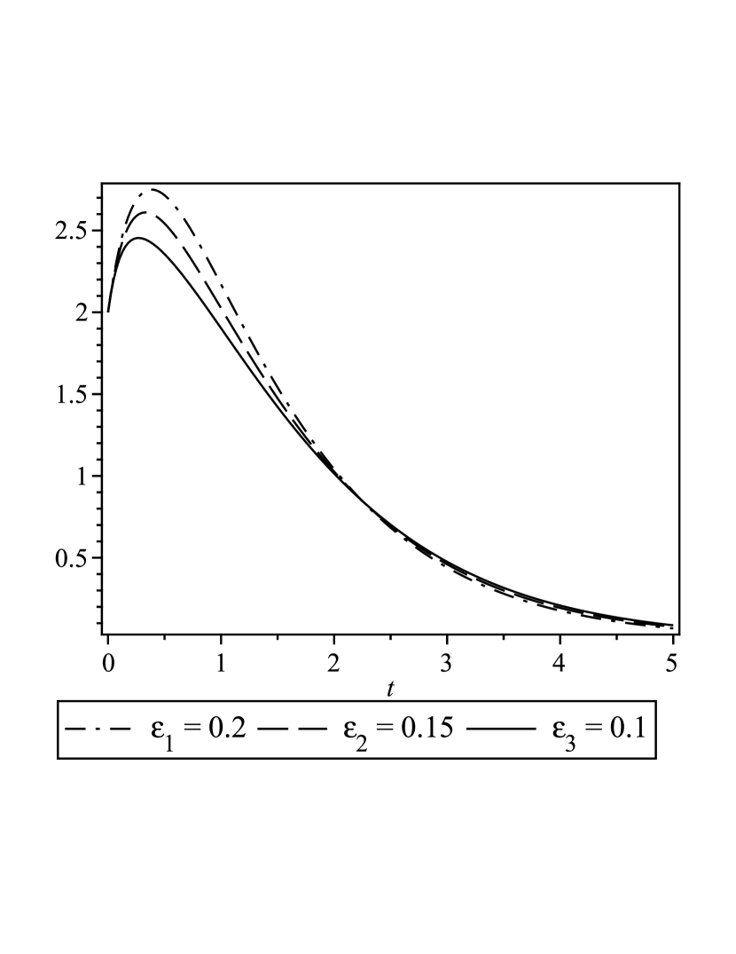
Figure 1: $x$-component of the trajectory of the system (131)-(132)

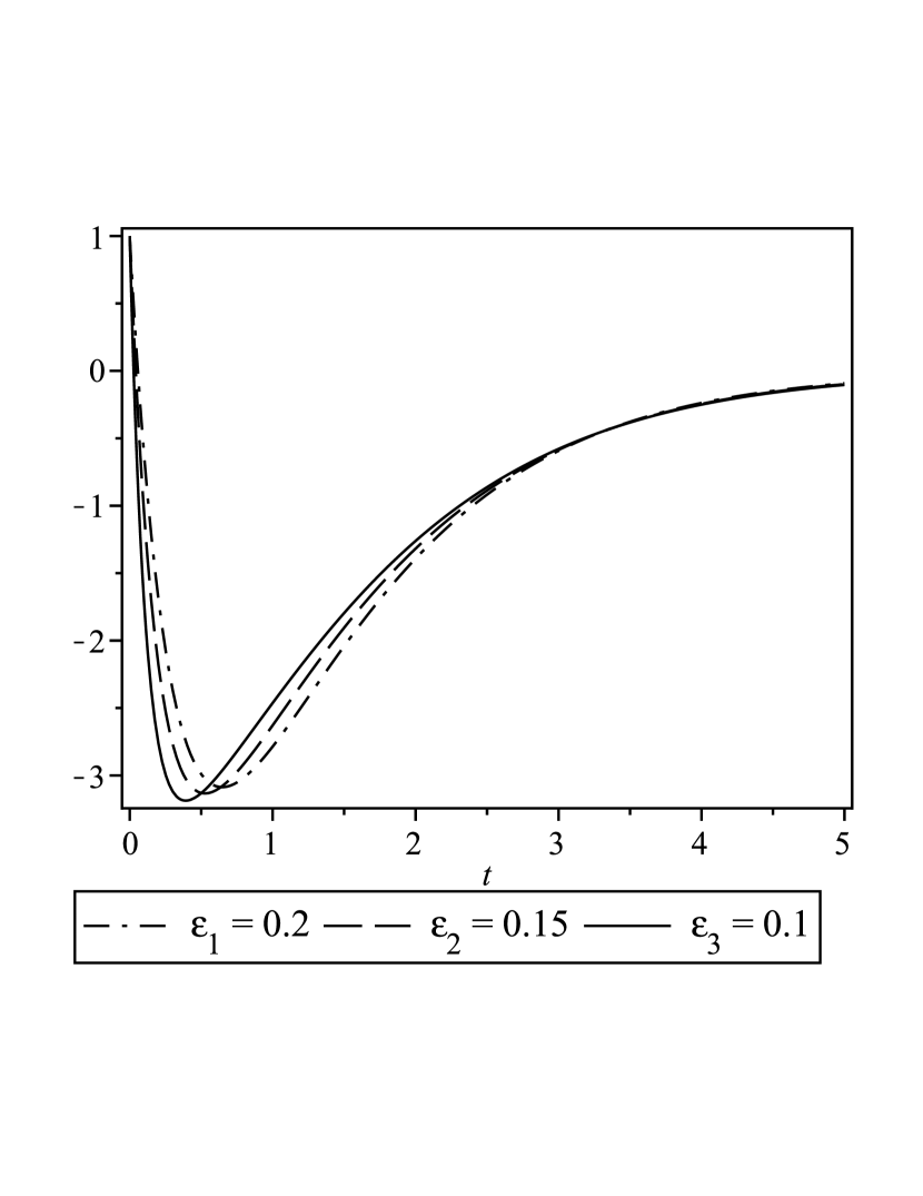
Figure 2: $y$-component of the trajectory of the system (131)-(132)

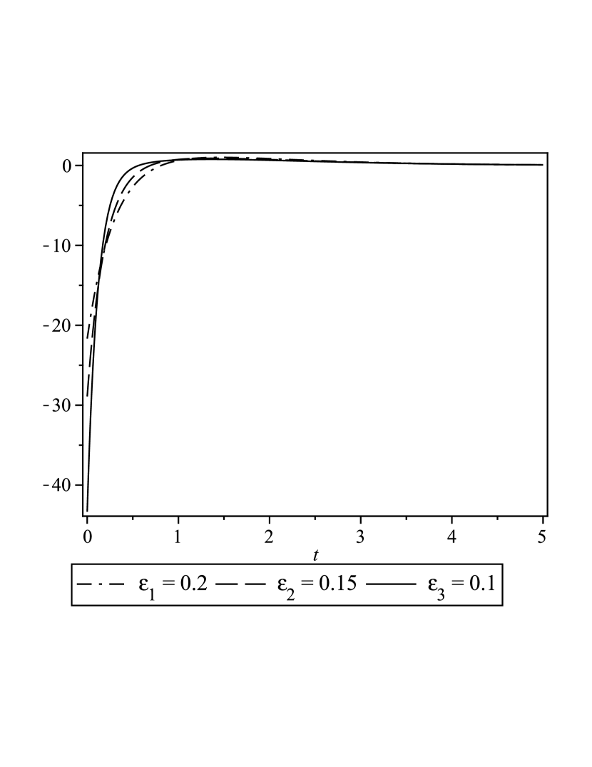
Figure 3: Time realization of $u_{\varepsilon_{k}}(z,t)$

In Figs. 1 and 2, the $x$- and $y$-components of the trajectory of the system (131)-(132), generated by the control (147) with different values of $\varepsilon_{k}$, are depicted for the following numerical data: $a_{1}=4$, $a_{2}=2$, $\gamma=1$, $x_{0}=2$, $y_{0}=1$, $d_{1}=2$, $d_{2}=1$. It is seen that both components tend to the components of the nominal trajectory for $t\rightarrow+\infty$. Moreover, for the smaller $\varepsilon_{k}$, the rate of this convergence is larger. In Fig. 3, the time realization of the control (147) along the trajectory of the system (131)-(132), depicted in Figs. 1–2, is presented. It is seen that for $\varepsilon_{k}$ approaching zero, this time realization tends to an impulse-like function with the impulse at $t=0$.

7 Concluding Remarks

CRI. In this paper, an infinite horizon linear-quadratic optimal control problem for a system with known time-varying additive disturbance is considered. A weight matrix of the control cost in the cost functional of this problem is singular but, in general, non-zero. Due to this singularity of the weight matrix, the optimal control problem itself is singular. However, if the weight matrix is non-zero, only a part of the coordinates of the control is singular, while the others are regular.
CRII. Subject to proper assumptions, the linear system of the control problem is transformed equivalently to a new system consisting of three modes. The first mode is uncontrolled directly (i.e. it does not contain the control at all), the second mode is controlled directly only by the regular coordinates of the control, while the third mode is controlled directly by the entire control. Due to this transformation, a new control problem, equivalent to the initially formulated one, is obtained. This new singular optimal control problem is considered as an original one in the paper.
CRIII. The original control problem is solved by a regularization approach, i.e., by its approximate transformation to an auxiliary regular optimal control problem. The latter has the same equation of dynamics and a similar cost functional augmented by an infinite horizon integral of the squares of the singular control coordinates with a small positive weight. Hence, the auxiliary problem is an infinite horizon linear-quadratic optimal control problem with partial cheap control. An asymptotic analysis of this problem is carried out.
CRIV. Based on this asymptotic analysis, it is shown that the infimum of the cost functional in the original (singular) optimal control problem is finite. The explicit expression of this infimum is derived. The minimizing state-feedback control sequence in the original problem also is designed. Some coordinates of the minimizing sequence are convergent in the class of regular functions. Namely, the coordinates of the minimizing sequence, corresponding to the regular control coordinates, are point-wise convergent in this class of functions. The corresponding limits constitute the regular part of the optimal state-feedback control in the original problem.
CRV. It is shown that the infimum of the cost functional and the regular part of the optimal state-feedback control in the original singular problem coincide with the optimal value of the cost functional and the upper block of the optimal state-feedback control, respectively, in a reduced dimension regular optimal control problem (reduced control problem). The dimension of the upper block of the optimal state-feedback control in the reduced control problem equals to the number of the regular coordinates of the control in the original problem. The reduced control problem is connected with the zero-order asymptotic solutions of the equations, arising in the optimality conditions of the auxiliary partial cheap control problem.
CRVI. Using the obtained theoretical results, the problem of singular infinite horizon trajectory tracking with two scalar state variables and a scalar control is solved. Numerical simulation shows that the state-feedback controls of the minimizing sequence generate trajectories, approaching well enough the nominal ones. The time-realizations of these state-feedback controls tend to an impulse-like function with the impulse at $t=0$.

8 Appendix A: Proof of Lemma 11

8.1 Auxiliary results

Let for a given $\varepsilon>0$, the matrix-valued function $\Psi(t,\varepsilon)$, $t\geq 0$ of the dimension $(m_{1}+m_{2})$ be the solution of the following initial-value problem:

$$\frac{d\Psi(t,\varepsilon)}{dt}=C(\varepsilon)\Psi(t,\varepsilon),\ \ \ \ \Psi(0,\varepsilon)=I_{m_{1}+m_{2}},$$ (148)

where a given $(m_{1}+m_{2})$-matrix $C(\varepsilon)$ has the block form

$$C(\varepsilon)=\left(\begin{array}[]{l}C_{1}(\varepsilon)\ \ \ \ \ \ \ \ \ \ C_{2}(\varepsilon)\\ (1/\varepsilon)C_{3}(\varepsilon)\ \ \ (1/\varepsilon)C_{4}(\varepsilon)\end{array}\right),$$ (149)

the blocks $C_{1}(\varepsilon)$, $C_{2}(\varepsilon)$, $C_{3}(\varepsilon)$ and $C_{4}(\varepsilon)$ are of the dimensions $m_{1}\times m_{1}$, $m_{1}\times m_{2}$, $m_{2}\times m_{1}$ and $m_{2}\times m_{2}$, respectively.

Represent the matrix $\Psi(t,\varepsilon)$ in the block form

$$\Psi(t,\varepsilon)=\left(\begin{array}[]{l}\Psi_{1}(t,\varepsilon)\ \ \ \ \Psi_{2}(t,\varepsilon)\\ \Psi_{3}(t,\varepsilon)\ \ \ \ \Psi_{4}(t,\varepsilon)\end{array}\right),$$ (150)

where the blocks $\Psi_{1}(t,\varepsilon)$, $\Psi_{2}(t,\varepsilon)$, $\Psi_{3}(t,\varepsilon)$, and $\Psi_{4}(t,\varepsilon)$ are of the dimensions $m_{1}\times m_{1}$, $m_{1}\times m_{2}$, $m_{2}\times m_{1}$ and $m_{2}\times m_{2}$, respectively.

Proposition 24

Let there exists a positive number $\check{\varepsilon}$ such that the matrices $C_{j}(\varepsilon)$, $(j=1,..4)$ are continuous with respect to $\varepsilon\in[0,\check{\varepsilon}]$. Let, there exists a positive number $\omega$ such that all the eigenvalues $\lambda\Big{(}C_{4}(\varepsilon)\Big{)}$ of the matrix $C_{4}(\varepsilon)$ satisfy the inequality

$$\mathrm{Re}\lambda\Big{(}C_{4}(\varepsilon)\Big{)}<-\omega,\ \ \ \ \varepsilon\in[0,\check{{\varepsilon}}].$$ (151)

Let, there exists a positive number $\kappa$ such that all the eigenvalues $\lambda\Big{(}\bar{C}(\varepsilon)\Big{)}$ of the matrix $\bar{C}(\varepsilon)\overset{\triangle}{=}C_{1}(\varepsilon)-C_{2}(\varepsilon)C_{4}^{-1}(\varepsilon)C_{3}(\varepsilon)$ satisfy the inequality

$$\mathrm{Re}\lambda\Big{(}\bar{C}(\varepsilon)\Big{)}<-\kappa,\ \ \ \ \varepsilon\in[0,\check{{\varepsilon}}].$$ (152)

Then, there exists a positive number $\bar{\varepsilon}$, ($\bar{\varepsilon}\leq\check{{\varepsilon}})$, such that for all $\varepsilon\in(0,\bar{\varepsilon}]$, the following inequalities are satisfied:

$$\big{\|}\Psi_{i}\big{(}t,\varepsilon\big{)}\big{\|}\leq a\exp\big{(}-\kappa t\big{)},\ \ \ \ i=1,3,\ \ \ \ 0\leq t<+\infty,$$ (153)

$$\big{\|}\Psi_{2}\big{(}t,\varepsilon\big{)}\big{\|}\leq a\varepsilon\exp\big{(}-\kappa t\big{)},\ \ \ \ 0\leq t<+\infty,$$ (154)

$$\big{\|}\Psi_{4}\big{(}t,\varepsilon\big{)}\big{\|}\leq a\Big{(}\varepsilon\exp\big{(}-\kappa t\big{)}+\exp\big{(}-\omega t/\varepsilon\big{)}\Big{)},\ \ \ \ 0\leq t<+\infty,$$ (155)

where $a>0$ is some constant independent of $\varepsilon$.

Proof. The statement of the proposition directly follows from the results of [35] (Theorem 2.3).   

Now, let us set $m_{1}=n-r+q$, $m_{2}=r-q$ and

$$C_{1}(\varepsilon)={\mathcal{A}}_{1}^{T}(\varepsilon),\ \ C_{2}(\varepsilon)={\mathcal{A}}_{3}^{T}(\varepsilon),\ \ C_{3}(\varepsilon)={\mathcal{A}}_{2}^{T}(\varepsilon),\ \ C_{4}(\varepsilon)={\mathcal{A}}_{4}^{T}(\varepsilon).$$ (156)

Corollary 25

Let the assumptions (A1)-(A3), (A5)-(A7) be valid. Then, there exists a positive number $\bar{\varepsilon}_{0}$, ($\bar{\varepsilon}_{0}\leq\varepsilon_{0}$), such that for all $\varepsilon\in(0,\bar{\varepsilon}_{0}]$ the following inequalities are satisfied:

$$\big{\|}\Psi_{i}\big{(}t,\varepsilon\big{)}\big{\|}\leq a\exp\big{(}-\alpha t\big{)},\ \ \ \ i=1,3,\ \ \ \ 0\leq t<+\infty,$$ (157)

$$\big{\|}\Psi_{2}\big{(}t,\varepsilon\big{)}\big{\|}\leq a\varepsilon\exp\big{(}-\alpha t\big{)},\ \ \ \ 0\leq t<+\infty,$$ (158)

$$\big{\|}\Psi_{4}\big{(}t,\varepsilon\big{)}\big{\|}\leq a\Big{(}\varepsilon\exp\big{(}-\alpha t\big{)}+\exp\big{(}-\beta t/\varepsilon\big{)}\Big{)},\ \ \ \ 0\leq t<+\infty,$$ (159)

where $a>0$ is some constant independent of $\varepsilon$.

Proof. First of all note that, due to the equations (70)-(73) and Lemma 10, the matrices $C_{j}(\varepsilon)$, $(j=1,..4)$, given by (156), are continuous with respect to $\varepsilon\in[0,\varepsilon_{0}]$.

Using the equations (42), (57), (70)-(73), (156) and Lemma 10, we obtain

$$C_{1}(\varepsilon)=A_{1}^{T}-P_{10}^{*}S_{1}+\Delta C_{1}(\varepsilon),$$ (160)

$$C_{2}(\varepsilon)=-P_{10}^{*}A_{2}\big{(}D_{2}\big{)}^{-1/2}+\Delta C_{2}(\varepsilon),$$ (161)

$$C_{3}(\varepsilon)=A_{2}^{T}+\Delta C_{3}(\varepsilon),$$ (162)

$$C_{4}(\varepsilon)=-\big{(}D_{2}\big{)}^{1/2}+\Delta C_{4}(\varepsilon),$$ (163)

where $\Delta C_{j}(\varepsilon)$, ($j=1,...,4$) are some matrices satisfying the inequalities

$$\big{\|}\Delta C_{j}(\varepsilon)\big{\|}\leq a\varepsilon,\ \ \ j=1,...,4.\ \ \ \varepsilon\in[0,\varepsilon_{0}],$$ (164)

$a>0$ is some constant independent of $\varepsilon$.

The equation (163) and the inequalities (58), (164) directly yield the existence of a positive number $\bar{\varepsilon}_{1}$, ($\bar{\varepsilon}_{1}\leq\varepsilon_{0}$), such that all the eigenvalues $\lambda\Big{(}C_{4}(\varepsilon)\Big{)}$ of the matrix $C_{4}(\varepsilon)$ satisfy the inequality

$$\mathrm{Re}\lambda\Big{(}C_{4}(\varepsilon)\Big{)}<-\beta,\ \ \ \ \varepsilon\in[0,\bar{\varepsilon}_{1}].$$ (165)

Now, based on (160)-(165) and (65), we immediately obtain that the matrix $\bar{C}(\varepsilon)=C_{1}(\varepsilon)-C_{2}(\varepsilon)C_{4}^{-1}(\varepsilon)C_{3}(\varepsilon)$ can be represented as:

$$\bar{C}(\varepsilon)={\mathcal{A}}_{0}^{T}+\overline{\Delta C}(\varepsilon),$$ (166)

where $\overline{\Delta C}(\varepsilon)$ is some matrix satisfying the inequality

$$\big{\|}\overline{\Delta C}(\varepsilon)\big{\|}\leq a\varepsilon,\ \ \ \ \varepsilon\in[0,\bar{\varepsilon}_{1}].$$ (167)

From the equation (166), and the inequalities (66) and (167), we directly obtain the existence of a positive number $\bar{\varepsilon}_{2}$, ($\bar{\varepsilon}_{2}\leq\bar{\varepsilon}_{1}$), such that all the eigenvalues $\lambda\Big{(}\bar{C}(\varepsilon)\Big{)}$ of the matrix $\bar{C}(\varepsilon)$ satisfy the inequality

$$\mathrm{Re}\lambda\Big{(}\bar{C}(\varepsilon)\Big{)}<-\alpha,\ \ \ \ \varepsilon\in[0,\bar{\varepsilon}_{2}].$$ (168)

Thus, we have shown that the blocks (156) of the matrix $C(\varepsilon)$ satisfy all the conditions of Proposition 24, which completes the proof of the corollary.   

8.2 Main part of the proof

Let $\Delta_{1}(t,\varepsilon)$ and $\Delta_{2}(t,\varepsilon)$ be vectors, defined as follows:

$$\Delta_{1}(t,\varepsilon)\overset{\triangle}{=}h_{1}(t,\varepsilon)-h_{10}(t),\ \ \ \Delta_{2}(t,\varepsilon)\overset{\triangle}{=}h_{2}(t,\varepsilon)-h_{20}(t),\ \ \ t\geq 0.$$ (169)

Substitution of (169) into (76)-(78), and using (79)-(80), (81) and (86) yield the problem for $\Delta_{1}(t,\varepsilon)$ and $\Delta_{2}(t,\varepsilon)$

$$\frac{d\Delta_{1}(t,\varepsilon)}{dt}=-{\mathcal{A}}_{1}^{T}(\varepsilon)\Delta_{1}(t,\varepsilon)-{\mathcal{A}}_{3}^{T}(\varepsilon)\Delta_{2}(t,\varepsilon)+\Gamma_{1}(t,\varepsilon),$$ (170)

$$\varepsilon\frac{d\Delta_{2}(t,\varepsilon)}{dt}=-{\mathcal{A}}_{2}^{T}(\varepsilon)\Delta_{1}(t,\varepsilon)-{\mathcal{A}}_{4}^{T}(\varepsilon)\Delta_{2}(t,\varepsilon)+\Gamma_{2}(t,\varepsilon),$$ (171)

$$\Delta_{1}(+\infty,\varepsilon)=0,\ \ \ \ \ \Delta_{2}(+\infty,\varepsilon)=0,$$ (172)

where

$$\Gamma_{1}(t,\varepsilon)=\big{(}{\mathcal{A}}_{1}^{T}(0)-{\mathcal{A}}_{1}^{T}(\varepsilon)\big{)}h_{10}(t)+\big{(}{\mathcal{A}}_{3}^{T}(0)-{\mathcal{A}}_{3}^{T}(\varepsilon)\big{)}h_{20}(t)$$

$$+\big{(}P_{10}^{*}-P_{1}^{*}(\varepsilon)\big{)}f_{1}(t)-\varepsilon P_{2}^{*}(\varepsilon)f_{2}(t),$$ (173)

$$\Gamma_{2}(t,\varepsilon)=\big{(}{\mathcal{A}}_{2}^{T}(0)-{\mathcal{A}}_{2}^{T}(\varepsilon)\big{)}h_{10}(t)+\big{(}{\mathcal{A}}_{4}^{T}(0)-{\mathcal{A}}_{4}^{T}(\varepsilon)\big{)}h_{20}(t)$$

$$-\varepsilon\big{(}P_{2}^{*}(\varepsilon)\big{)}^{T}f_{1}(t)-\varepsilon P_{3}^{*}(\varepsilon)f_{2}(t).$$ (174)

Using the equations (42)-(46), (70)-(73), Lemma 10 (the inequalities (68)), and the inequalities (18), (85), (87), we directly have

$$\big{\|}\Gamma_{i}(t,\varepsilon)\big{\|}\leq a\varepsilon\exp(-\gamma t),\ \ \ \ i=1,2,\ \ \ \ t\geq 0,\ \ \ \varepsilon\in(0,\tilde{\varepsilon}_{0}],$$ (175)

where $\tilde{\varepsilon}_{0}\overset{\triangle}{=}\min\{1,\varepsilon_{0}\}$; $a>0$ is some constant independent of $\varepsilon$.

Using the equations (148)-(150) and (156), we can represent the solution of the problem (170)-(172) as follows:

$$\Delta_{1}(t,\varepsilon)=\int_{0}^{+\infty}\Big{(}\Psi_{1}(\sigma,\varepsilon)\Gamma_{1}(\sigma+t,\varepsilon)+(1/\varepsilon)\Psi_{2}(\sigma,\varepsilon)\Gamma_{2}(\sigma+t,\varepsilon)\Big{)}d\sigma,\ t\geq 0,$$ (176)

$$\Delta_{2}(t,\varepsilon)=\int_{0}^{+\infty}\Big{(}\Psi_{3}(\sigma,\varepsilon)\Gamma_{1}(\sigma+t,\varepsilon)+(1/\varepsilon)\Psi_{4}(\sigma,\varepsilon)\Gamma_{2}(\sigma+t,\varepsilon)\Big{)}d\sigma,\ t\geq 0.$$ (177)

These equations, along with the inequalities (157)-(159) and (175), directly yield the inequalities

$$\big{\|}\Delta_{i}(t,\varepsilon)\big{\|}\leq c\varepsilon\exp(-\mu t),\ \ \ \ i=1,2,\ \ \ t\geq 0,\ \ \ \varepsilon\in(0,\varepsilon_{1}],$$ (178)

where $\varepsilon_{1}=\min\{\bar{\varepsilon}_{0},\tilde{\varepsilon}_{0}\}$, $c>0$ is some constant independent of $\varepsilon$.

The equation (169) and the inequalities (178) immediately imply the inequalities (88). This completes the proof of the lemma.

9 Appendix B: Proof of Lemma 18

We prove the lemma for $u_{\varepsilon,1}(z,t)$. The admissibility of $u_{\varepsilon,2}(z,t)$ is shown similarly.

Substitution of $u_{\varepsilon,1}\left(z,t\right)$ into (9), and using the equations (30), (36)-(46), (49), (74), (96) and (109) yield the following initial-value problem in the interval $t\in[0,+\infty)$:

$$\frac{dx(t)}{dt}={\mathcal{A}}_{10}(\varepsilon)x(t)+{\mathcal{A}}_{20}(\varepsilon)y(t)-S_{1}h_{10}(t)-\varepsilon S_{2}h_{20}(t)+f_{1}(t),\ \ \ x(0)=x_{0},$$ (179)

$$\varepsilon\frac{dy(t)}{dt}={\mathcal{A}}_{30}(\varepsilon)x(t)+{\mathcal{A}}_{40}(\varepsilon)y(t)$$

$$-\varepsilon S_{2}^{T}h_{10}(t)-S_{3}(\varepsilon)h_{20}(t)+\varepsilon f_{2}(t),\ \ \ y(0)=y_{0},$$ (180)

where

$${\mathcal{A}}_{10}(\varepsilon)=A_{1}-S_{1}P^{*}_{10}-\varepsilon S_{2}\big{(}P^{*}_{20}\big{)}^{T},$$ (181)

$${\mathcal{A}}_{20}(\varepsilon)=A_{2}-\varepsilon S_{1}P^{*}_{20}-\varepsilon S_{2}P^{*}_{30},$$ (182)

$${\mathcal{A}}_{30}(\varepsilon)=\varepsilon A_{3}-\varepsilon S_{2}P^{*}_{10}-S_{3}(\varepsilon)\big{(}P^{*}_{20}\big{)}^{T},$$ (183)

$${\mathcal{A}}_{40}(\varepsilon)=\varepsilon A_{4}-\varepsilon^{2}S_{2}^{T}P^{*}_{20}-S_{3}(\varepsilon)P^{*}_{30}.$$ (184)

For any $\varepsilon\in(0,\varepsilon_{0}]$, the problem (179)-(180) has the unique locally absolutely continuous solution $z(t,\varepsilon)=\{x(t,\varepsilon),y(t,\varepsilon)\}$, $t\in[0,+\infty)$.

Using the inequalities (18), (85), (87), one can obtain (similarly to the inequalities (178)) the following inequalities:

$$\|x(t,\varepsilon)\|\leq a\exp(-\mu t),\ \ \ \ \|y(t,\varepsilon)\|\leq a\exp(-\mu t),\ \ \ t\geq 0,\ \ \ \ \varepsilon\in(0,\check{{\varepsilon}}_{1}],$$ (185)

where $\check{{\varepsilon}}_{1}>0$, ($\check{{\varepsilon}}_{1}\leq\varepsilon_{2}$) is some constant; $a>0$ is some constant independent of $\varepsilon$; the constant $\mu$ is given by (89).

Due to (185), $z(t,\varepsilon)\in L^{2}[0,+\infty;E^{n}]$ for all $\varepsilon\in(0,\check{{\varepsilon}}_{1}]$. The latter inclusion, along with the equation (106), yields the inclusion $u_{\varepsilon,1}\big{(}z(t,\varepsilon),t\big{)}\in L^{2}[0,+\infty;E^{r}]$ for all $\varepsilon\in(0,\check{{\varepsilon}}_{1}]$. Thus, the state-feedback control $u_{\varepsilon,1}(z,t)$ satisfies all the conditions of the admissibility in the OOCP, which completes the proof of the lemma.

10 Appendix C: Proof of Theorem 21

We prove the theorem for the sequence $\{u_{\varepsilon_{k},1}(z,t)\}$, ($k=1,2,...$). The statement of the theorem with respect to the sequence $\{u_{\varepsilon_{k},2}(z,t)\}$, ($k=1,2,...$) is proven similarly.

10.1 Auxiliary results

Similarly to proof of Lemma 18 (see Section 9), the substitution of $u_{\varepsilon,1}\left(z,t\right)$ into (9) yields the initial-value problem (179)-(180) in the interval $t\in[0,+\infty)$. Let us construct the zero-order asymptotic solution to this problem. Following the Boundary Function Method [36], we look for this asymptotic solution in the form

$$x_{0}^{\mathrm{as}}(t,\varepsilon)=x_{0}^{o}(t)+x_{0}^{b}(\tau),\ \ \ \ y_{0}^{\mathrm{as}}(t,\varepsilon)=y_{0}^{o}(t)+y_{0}^{b}(\tau),\ \ \ \tau=t/\varepsilon,$$ (186)

where $\{x_{0}^{o}(t),y_{0}^{o}(t)\}$ is the so-called outer solution, $x_{0}^{b}(\tau)$ and $y_{0}^{b}(\tau)$ are the boundary correction terms.

Equations and conditions for obtaining the asymptotic solution (186) are derived by substitution of $x_{0}^{\mathrm{as}}(t,\varepsilon)$ and $y_{0}^{\mathrm{as}}(t,\varepsilon)$ into the problem (179)-(180) instead of $x(t)$ and $y(t)$, respectively, and equating the coefficients for the same powers of $\varepsilon$ on both sides of the resulting equations, separately for the outer solution terms and the boundary correction terms.

10.1.1 Obtaining $x_{0}^{b}(\tau)$

For obtaining this term, we derive the equation

$$\frac{dx_{0}^{b}(\tau)}{d\tau}=0,\ \ \ \ \tau\geq 0.$$ (187)

Due to the Boundary Function Method, we require that $x_{0}^{b}(\tau)\rightarrow 0$ for $\tau\rightarrow+\infty$. Subject to this requirement, the equation (187) yields the unique solution

$$x_{0}^{b}(\tau)\equiv 0,\ \ \ \ \tau\geq 0.$$ (188)

10.1.2 Obtaining the outer solution

Using the equations (42)-(46), (57), (82) and (181)-(184), we have the system for $\{x_{0}^{o}(t),y_{0}^{o}(t)\}$

$$\frac{dx_{0}^{o}(t)}{dt}=\big{(}A_{1}-S_{1}P_{10}^{*}\big{)}x_{0}^{o}(t)+A_{2}y_{0}^{o}(t)-S_{1}h_{10}(t)+f_{1}(t),$$ (189)

$$0=-\big{(}D_{2}\big{)}^{-1/2}A_{2}^{T}P_{10}^{*}x_{0}^{o}(t)-\big{(}D_{2}\big{)}^{1/2}y_{0}^{o}(t)-\big{(}D_{2}\big{)}^{-1/2}A_{2}^{T}h_{10}(t).$$ (190)

Solving the equation (190) with respect to $y_{0}^{o}(t)$, we obtain

$$y_{0}^{o}(t)=-D_{2}^{-1}A_{2}^{T}P_{10}^{*}x_{0}^{o}(t)-D_{2}^{-1}A_{2}^{T}h_{10}(t).$$ (191)

Then, substituting (191) into (189), and using (60) and (65) yields the differential equation with respect to $x_{0}^{o}(t)$

$$\frac{dx_{0}^{o}(t)}{dt}={\mathcal{A}}_{0}x_{0}^{o}(t)-S_{0}h_{10}(t)+f_{1}(t).$$ (192)

Moreover, using (188), we directly have the initial condition for this equation

$$x_{0}^{o}(0)=x_{0}.$$ (193)

The solution of the problem (192)-(193) is

$$x_{0}^{o}(t)=\exp\big{(}{\mathcal{A}}_{0}t\big{)}x_{0}$$

$$-\int_{0}^{t}\exp\big{(}{\mathcal{A}}_{0}(t-\sigma)\big{)}\Big{(}S_{0}h_{10}(\sigma)-f_{1}(\sigma)\Big{)}d\sigma,\ \ \ \ t\geq 0.$$ (194)

Due to (18), (66), (85) and (89), this solution satisfies the inequality

$$\big{\|}x_{0}^{o}(t)\big{\|}\leq a\exp(-\mu t),\ \ \ \ t\geq 0,$$ (195)

where $a>0$ is some constant.

The equations (89), (191), and the inequalities (85), (195) yield

$$\big{\|}y_{0}^{o}(t)\big{\|}\leq a\exp(-\mu t),\ \ \ \ t\geq 0,$$ (196)

where $a>0$ is some constant.

10.1.3 Obtaining $y_{0}^{b}(\tau)$

Using (42)-(46), (57), (184), we have the following equation for this boundary correction term:

$$\frac{dy_{0}^{b}(\tau)}{d\tau}=-\big{(}D_{2}\big{)}^{1/2}y_{0}^{b}(\tau),\ \ \ \ \tau\geq 0.$$ (197)

Moreover, the initial condition for this equation is

$$y_{0}^{b}(0)=y_{0}-y_{0}^{o}(0).$$ (198)

The solution of the problem (197)-(198) has the form

$$y_{0}^{b}(\tau)=\exp\Big{(}-\big{(}D_{2}\big{)}^{1/2}t\Big{)}\big{(}y_{0}-y_{0}^{o}(0)\big{)},\ \ \ \ \tau\geq 0.$$ (199)

Due to (58), this solution satisfies the inequality

$$\big{\|}y_{0}^{b}(\tau)\big{\|}\leq a\exp(-\beta\tau),\ \ \ \ \tau\geq 0,$$ (200)

where $a>0$ is some constant.

Thus, we have completed the formal construction of the zero-order asymptotic solution to the problem (179)-(180).

Lemma 26

Let the assumptions (A1)-(A7) be valid. Then, there exists a positive constant $\tilde{\varepsilon}_{1}$, ($\tilde{\varepsilon}_{1}\leq\varepsilon_{2}$), such that for all $\varepsilon\in(0,\tilde{\varepsilon}_{1}]$ the solution $\{x(t,\varepsilon),y(t,\varepsilon)\}$ of the initial-value problem (179)-(180) satisfies the inequalities

$$\big{\|}x(t,\varepsilon)-x_{0}^{o}(t)\big{\|}\leq c\varepsilon\exp(-\mu t),\ \ \ \ \ t\geq 0,$$ (201)

$$\big{\|}y(t,\varepsilon)-y_{0}^{o}(t)-y_{0}^{b}(t/\varepsilon)\big{\|}\leq c\varepsilon\exp(-\mu t),\ \ t\geq 0,$$ (202)

where $c>0$ is some constant independent of $\varepsilon$.

Proof. The lemma is proven similarly to Lemma 11.   

Let us denote

$$J_{0}\overset{\triangle}{=}\int_{0}^{+\infty}\Big{[}\big{(}x_{0}^{o}(t)\big{)}^{T}D_{1}x_{0}^{o}(t)$$

$$+\Big{(}P_{10}^{*}x_{0}^{o}(t)+h_{10}(t)\Big{)}^{T}S_{0}\Big{(}P_{10}^{*}x_{0}^{o}(t)+h_{10}(t)\Big{)}\Big{]}dt.$$ (203)

Corollary 27

Let the assumptions (A1)-(A7) be valid. Then, for all $\varepsilon\in(0,\tilde{\varepsilon}_{1}]$ the following inequality is satisfied:

$$\big{|}J\big{(}u_{\varepsilon,1}(z,t)\big{)}-J_{0}\big{|}\leq c\varepsilon.$$ (204)

Proof. Substitution of $z(t,\varepsilon)=\mathrm{col}\big{(}x(t,\varepsilon),x(t,\varepsilon)\big{)}$ and $u_{\varepsilon,1}\big{(}z(t,\varepsilon),t\big{)}$ (see (107)) into (10), and using (3) and (15) yields

$$J\big{(}u_{\varepsilon,1}(z,t)\big{)}=\int_{0}^{+\infty}\Big{[}x^{T}(t,\varepsilon)D_{1}x(t,\varepsilon)+y^{T}(t,\varepsilon)D_{2}y(t,\varepsilon)$$

$$+\big{(}K_{1}(\varepsilon)x+\varepsilon K_{2}(\varepsilon)y+H_{3}h_{10}(t)+\varepsilon H_{1}h_{20}(t)\big{)}^{T}\widetilde{G}$$

$$\times\big{(}K_{1}(\varepsilon)x+\varepsilon K_{2}(\varepsilon)y+H_{3}h_{10}(t)+\varepsilon H_{1}h_{20}(t)\big{)}\Big{]}dt,$$ (205)

where $\widetilde{G}$ is given in (46).

Now, using the equations (108), Lemma 26 and the inequalities (195), (196), (200), we can represent the expression (10.1.3) as follows:

$$J\big{(}u_{\varepsilon,1}(z,t)\big{)}=\int_{0}^{+\infty}\Big{[}\big{(}x_{0}^{o}(t)\big{)}^{T}D_{1}x_{0}^{o}(t)+\big{(}y_{0}^{o}(t)\big{)}^{T}D_{2}y_{0}^{o}(t)$$

$$+\big{(}P_{10}x_{0}^{o}(t)+h_{10}(t)\big{)}^{T}H_{3}^{T}\widetilde{G}H_{3}\big{(}P_{10}x_{0}^{o}(t)+h_{10}(t)\big{)}\big{]}dt+l(\varepsilon),$$ (206)

where $l(\varepsilon)$ is some function of $\varepsilon$ satisfying the inequality

$$\|l(\varepsilon)\|\leq c\varepsilon,\ \ \ \ \varepsilon\in(0,\tilde{\varepsilon}_{1}],$$ (207)

$c>0$ is some constant independent of $\varepsilon$.

Now, using (191), we have

$$\big{(}y_{0}^{o}(t)\big{)}^{T}D_{2}y_{0}^{o}(t)=\big{(}P_{10}x_{0}^{o}(t)+h_{10}(t)\big{)}^{T}A_{2}D_{2}^{-1}A_{2}^{T}\big{(}P_{10}x_{0}^{o}(t)+h_{10}(t)\big{)}.$$ (208)

Also, using (42)-(46), we obtain

$$H_{3}^{T}\widetilde{G}H_{3}=S_{1}.$$ (209)

Finally, the substitution of (208)-(209) into (10.1.3), and using the equation (60) and the inequality (207) lead immediately to the inequality (202). Thus, the corollary is proven.   

10.2 Main part of the proof

Substitution of the optimal control (101) of the ROCP into the dynamics (99) of this problem, and using the equations (61), (65) yields after some rearrangement the following initial-value problem for the optimal trajectory $\bar{x}^{\ast}(t)$, $t\geq 0$ in the ROCP:

$$\frac{d\bar{x}^{\ast}(t)}{dt}={\mathcal{A}}_{0}\bar{x}^{\ast}(t)-S_{0}h_{10}(t)+f_{1}(t),\ \ \ \ \bar{x}^{\ast}(0)=x_{0}.$$ (210)

Comparison of this problem with the problem (192)-(193) yields

$$\bar{x}^{\ast}(t)\equiv x_{0}^{o}(t),\ \ \ \ t\geq 0.$$ (211)

Replacing $\bar{x}$ with $x_{0}^{o}(t)$ in (101), we obtain the time realization $\bar{u}^{\ast}(t)$ of the optimal state-feedback control in the ROCP

$$\bar{u}^{\ast}(t)=-\Theta^{-1}\bar{B}^{T}P_{10}^{\ast}x_{0}^{o}(t)-\Theta^{-1}\bar{B}^{T}h_{10}(t),\ \ \ \ t\geq 0.$$ (212)

Now, substituting (211) and (212) into (100) instead of $\bar{x}(t)$ and $\bar{u}(t)$, respectively, and using (61) yield the equality

$$\bar{J}^{\ast}=J_{0},$$ (213)

where $\bar{J}^{\ast}$ is the optimal value of the cost functional in the ROCP, while the value $J_{0}$ is given by (10.1.3). Finally, the equalities (112), (213) and the inequality (204) directly imply the statement of the theorem.

References

- [1] Pontriagin, L.S., Boltyanskii, V.G., Gamkrelidze, R.V., Mischenko, E.F.: The Mathematical Theory of Optimal Processes, Gordon Breach, New York (1986)
- [2] Bellman, R.: Dynamic Programming, Princeton University Press, Princeton, NJ (1957)
- [3] Kelly, H. J.: A second variation test for singular extremals. AIAA Journal 2, 26–29 (1964)
- [4] Bell, D.J., Jacobson, D.H.: Singular Optimal Control Problems, Academic Press, New York (1975)
- [5] Gabasov, R., Kirillova, F.M.: High order necessary conditions for optimality. SIAM J. Control 10, 127–168 (1972)
- [6] Mehrmann, V.: Existence, uniqueness, and stability of solutions to singular linear quadratic optimal control problems. Linear Algebra Appl. 121, 291–331 (1989)
- [7] Krotov, V.F.: Global Methods in Optimal Control Theory, Marsel Dekker, New York (1996)
- [8] Ferrante, A., Ntogramatzidis, L,: Continuous-time singular linear-quadratic control: necessary and sufficient conditions for the existence of regular solutions. arXiv:1404.1667v1 [math.OC], 12 p (2014)
- [9] Gurman, V.I.: Optimal processes of singular control. Autom. Remote Control 26, 783—792 (1965)
- [10] Gurman, V.I., Dykhta, V.A.: Singular problems of optimal control and the method of multiple maxima. Autom. Remote Control 38, 343—350 (1977)
- [11] Gurman, V.I., Ni Ming Kang: Degenerate problems of optimal control. I. Autom. Remote Control 72, 497–511 (2011)
- [12] Gurman, V.I., Ni Ming Kang: Degenerate problems of optimal control. II. Autom. Remote Control 72, 727—739 (2011)
- [13] Gurman, V.I., Ni Ming Kang: Degenerate problems of optimal control. III. Autom. Remote Control 72, 929—-943 (2011)
- [14] Hautus, M.L.J., Silverman, L.M.: System structure and singular control. Linear Algebra Appl. 50, 369–402 (1983)
- [15] Willems, J.C., Kitapci, A., Silverman, L.M.: Singular optimal oontrol: a geometric approach. SIAM J. Control Optim. 24, 323—337 (1986)
- [16] Geerts, T.: All optimal controls for the singular linear-quadratic problem without stability; a new interpretation of the optimial cost. Linear Algebra Appl. 116, 135-181 (1989)
- [17] Geerts, T.: Linear-quadratic control with and without stability subject to general implicit continuous-time systems: coordinate-free interpretations of the optimal costs in terms of dissipation inequality and linear matrix inequality; existence and uniqueness of optimal controls and state trajectories. Linear Algebra Appl. 203-204, 607-658 (1994)
- [18] Zavalishchin, S.T., Sesekin, A.N.: Dynamic Impulse Systems: Theory and Applications, Kluwer Academic Publishers, Dordrecht (1997)
- [19] Glizer, V.Y.: Solution of a singular optimal control problem with state delays: a cheap control approach. In: Reich, S., Zaslavski, A.J. (eds.): Optimization Theory and Related Topics, Contemporary Mathematics Series, vol. 568, pp. 77–107. American Mathematical Society, Providence, RI (2012)
- [20] Glizer, V.Y.: Stochastic singular optimal control problem with state delays: regularization, singular perturbation, and minimizing sequence. SIAM J. Control Optim. 50, 2862–2888 (2012)
- [21] Glizer, V.Y. Singular solution of an infinite horizon linear-quadratic optimal control problem with state delays. In: Wolansky, G., Zaslavski, A.J. (eds.): Variational and Optimal Control Problems on Unbounded Domains, Contemporary Mathematics Series, vol. 619, pp. 59–98. American Mathematical Society, Providence, RI (2014)
- [22] Tikhonov, A.N., Arsenin, V.Y.: Solutions of Ill-Posed Problems, Halsted Press, New York (1977)
- [23] Glizer, V.Y., Fridman, L.M., Turetsky, V.: Cheap suboptimal control of an integral sliding mode for uncertain systems with state delays. IEEE Trans. Automat. Control, 52, 1892–1898 (2007)
- [24] Glizer, V.Y., Kelis, O.: Solution of a zero-sum linear quadratic differential game with singular control cost of minimizer. Journal of Control and Decision, 2, 155–184 (2015)
- [25] O’Malley, R.E., Jameson, A.: Singular perturbations and singular arcs, II. IEEE Trans. Automat. Control 22, 328–337 (1977)
- [26] Sabery, A., Sannuti, P.: Cheap and singular controls for linear quadratic regulators. IEEE Trans. Automat. Control 32, 208–219 (1987)
- [27] Seron, M.M., Braslavsky, J.H., Kokotovic, P.V., Mayne, D.Q.: Feedback limitations in nonlinear systems: from Bode integrals to cheap control. IEEE Trans. Automat. Control 44, 829-833 (1999)
- [28] Glizer, V.Y.: Asymptotic solution of a cheap control problem with state delay. Dynam. Control, 9, 339–357 (1999)
- [29] Smetannikova, E.N., Sobolev, V.A.: Regularization of cheap periodic control problems. Automat. Remote Control 66, 903–916 (2005)
- [30] Glizer, V.Y.: Infinite horizon cheap control problem for a class of systems with state delays. J. Nonlinear Convex Anal. 10, 199–233 (2009)
- [31] O’Reilly, J.: Partial cheap control of the time-invariant regulator. Internat. J. Control 37, 909–927 (1983)
- [32] Salukvadze, M.E.: The analytical design of an optimal control in the case of constantly acting disturbances. Automat. Remote Control 23, 657–667 (1962)
- [33] Anderson, B.O.D, Moore, J.B.: Linear Optimal Control, Prentice-Hall, Englewood, NJ (1971)
- [34] Kokotovic, P.V., Khalil, H.K., O’ Reilly, J.: Singular Perturbation Methods in Control: Analysis and Design, Academic Press, London, UK (1986)
- [35] Glizer, V.Y.: Blockwise estimate of the fundamental matrix of linear singularly perturbed differential systems with small delay and its application to uniform asymptotic solution. J. Math. Anal. Appl. 278, 409-433 (2003)
- [36] Vasil’eva, A.B., Butuzov, V.F., Kalachev, L.V.: The Boundary Function Method for Singular Perturbation Problems, SIAM Books, Philadelphia, PA: (1995)