Spatiotemporal Evolution of Topological Order Upon Quantum Quench Across the Critical Point

Abstract

We consider a topological superconducting wire and use the string order parameter to investigate the spatiotemporal evolution of the topological order upon a quantum quench across the critical point. We also analyze the propagation of the initially localized Majorana bound states after the quench, in order to examine the connection between the topological order and the unpaired Majorana states, which has been well established at equilibrium but remains illusive in dynamical situations. It is found that after the quench the string order parameters decay over a finite time and that the decaying behavior is universal, independent of the wire length and the final value of the chemical potential (the quenching parameter). It is also found that the topological order is revived repeatedly although the amplitude gradually decreases. Further, the topological order can propagate into the region which was initially in the non-topological state. It is observed that all these behaviors are in parallel and consistent with the propagation and dispersion of the Majorana wave functions. Finally, we propose a local probing method which can measure the non-local topological order.

1 Introduction

Traditionally, Landau’s symmetry-breaking theory [1, 2, 3] has long provided a universal paradigm for the states of matter and their transitions. In this paradigm, continuous phase transitions are driven by the spontaneous symmetry breaking and naturally described by local order parameters. In recent decades, condensed-matter physics has witnessed the breakdown of the symmetry-breaking theory in describing symmetry-protected topological states. One of the most common and earliest examples is the quantum Hall effect [4, 5], where different quantum Hall states have the same symmetry. Topological phase transitions involve the change in internal topology rather than symmetry breaking [6, 7]. Necessarily, topological states are classified by topological quantum numbers. For example, different quantum Hall states are classified by the topological Chern number [8, 9], and topological insulators and superconductors are characterized by the number of gapless boundary (surface, edge or endpoint) states [10, 11, 7, 12] separated from gapped bulk states.

From the dynamical point of view, the classification in terms of discrete topological quantum numbers puts a serious limitation. For example, let us ask the question, how long does it take for a topological order to form? Namely, how does the topological order emerge or disappear temporally when system parameters are quenched across the critical point? Within Landau’s paradigm, the approach to the corresponding questions is conceptually clear because the local order parameters take continuous values and their dynamics are governed by a differential equation of motion, so called the time-dependent Ginzburg-Landau equation [13, 14, 15].

Another conceptual difficulty in the dynamical description of topological order arises from the fact that the topological quantum numbers or similar classifications concern about the ground state(s). In order to describe the full aspects of the temporal evolution of the topological order, one has to take into account the excited states as well as the ground states.

To overcome these issues in the dynamical theory of topological order, a few different approaches have been carried out previously: In Ref. [16], the fidelity of the final state with respect to the initial state has been examined. Similarly, the survival and revival probabilities [17, 18] or the Loschmidt echo [19] of the Majorana states after the quench have been also investigated. In particular, the sudden coupling of the localized Majorana state to the normal metallic (gapless) lead gives rise to universal features in the evolution of the Majorana wave function [19]. For a ladder system studied in Ref. [20], the number of excited vortices in plaquettes was inspected. It has also been suggested to use the Kibble-Zurek mechanism, which was originally put forward to study the cosmological phase transitions of the early Universe [21, 22] and later extended to classical phase transitions [23, 24]. This approach is particularly simple and insightful as it is only based on the competition between the internal and driving time scales. It has been shown that the original Kibble-Zurek scaling form does not hold for the topological phase transitions [25, 26] but one can generalize it by properly taking into account the multi-level structure due to the Majorana bound states [27].

However, none of these approaches directly measures the dynamic topological order; they either resort to the fidelity to the ground state or to the number of topological defects. Here we note that in one spatial dimension one can draw a close analogy with the conventional order by introducing a continuous parameter for the topological order [28]. The cost is that unlike the conventional order parameter the so-called string order parameter for the topological order is nonlocal: It is defined as the the expectation value of a product of consecutive Majorana operators in a certain range with respect to the dynamical wave function. It naturally captures the dynamical evolution of the topological order reflected in the wave function, and is considered to be more suitable for experimental observations [28].

On these grounds, in this work we adopt the string order parameter [29, 30, 31] to investigate the spatiotemporal evolution of the topological order upon a quantum quench across the critical point in a topological superconducting wire [32, 33, 34, 35]. In addition, we separately analyze the propagation of the initially localized Majorana bound states after quenching. By comparing the propagations of the topological order and the Majorana states, we examine the connection between them in the dynamical situations. It is stressed that while the close connection between the topological order and the Majorana bound states has been well established for the ground state, i.e., at equilibrium [32, 33, 34, 35], it is not obvious at all in the dynamical situations, which involve excited states.

We find that after the quench toward the nontopological phase, the string order parameters decay over a finite time before they vanish completely. Notably, this early decaying behavior is universal in the sense that it does not depend on the wire length and the final value of the chemical potential (the quenched parameter). We also find that the topological order is revived repeatedly although the amplitude gradually decreases. More interestingly, the topological order propagates into the regions which were initially prepared in the non-topological state. It is observed that all these behaviors of the dynamical topological order are in parallel and consistent with the propagation and dispersion of the Majorana wave functions. Finally, we propose a local probing method which can measure the topological order which is nonlocal in nature.

The rest of the paper is organized as following: Section 2 describes the model Hamiltonian for the topological superconducting wire and defines the string order parameters. For later use, it summarizes the mathematical and physical properties of the string order parameters. Section 3 studies the time evolution of the string order parameter in a uniform wire. It discusses the dynamical aspects of the topological order in terms of the propagation of the Majorana wave functions. Section 4 investigate the case where only the central part of the superconducting wire is initially in the topological phase and the outer part is topologically trivial so that the propagation of the topological order is examined. Section 5 proposes possible experimental methods to observe our findings. Finally, Section 6 concludes the paper.

2 Topological Superconducting Wires and Topological Order

2.1 Model

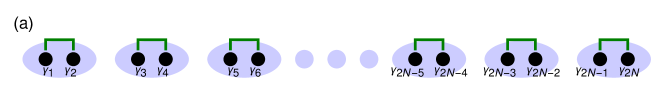
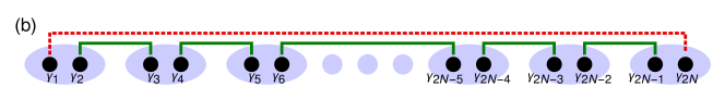
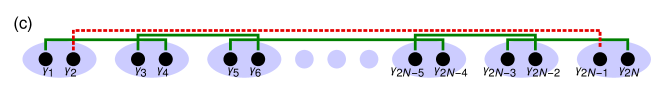
Figure 1: Majorana chain representation of one-dimensional topological superconducting wire. Each pair of Majorana fermions, $\gamma_{2j-1}$ and $\gamma_{2j}$ in a circle forms the site fermion $c_{j}$. The lines connecting Majorana fermions represent the coupling between them in three special conditions: (a) $w=\Delta=0$ and $\mu\neq 0$, (b) $\Delta=w$ and $\mu=0$, and (c) $\Delta=-w$ and $\mu=0$. The non-local correlations (red dotted lines) between otherwise isolated Majorana fermions arise only when the fermion parity condition is imposed.

In order to explore the time evolution of topological order under a quench, we consider Kitaev’s spinless $p$-wave topological superconducting wire with finite number of sites $N$ and with open ends described by the tight-binding Hamiltonian [32]

$$H(t) =\sum_{j=1}^{N-1}\frac{1}{2}\left(\Delta c_{j}c_{j+1}-wc_{j}^{\dagger}c_{j+1}+(h.c.)\right)-\sum_{j=1}^{N}\mu_{j}(t)\left(c_{j}^{\dagger}c_{j}-\frac{1}{2}\right)$$ (1a)

$$=\frac{i}{4}\sum_{j=1}^{N-1}\left[(\Delta+w)\gamma_{2j}\gamma_{2j+1}+(\Delta-w)\gamma_{2j-1}\gamma_{2j+2}\right]-\frac{i}{2}\sum_{j=1}^{N}\mu_{j}(t)\gamma_{2j-1}\gamma_{2j}$$ (1b)

with the hopping amplitude $w>0$, the superconducting gap $\Delta$, and the site-dependent chemical potential $\mu_{j}(t)$. The phase of the superconducting order parameter is neglected since it can be always gauged away. The fermion operator $c_{j}$ on site $j$ can be decomposed into the superposition of two Majorana fermion operators: $c_{j}=(\gamma_{2j-1}+i\gamma_{2j})/2$, satisfying $\gamma_{k}=\gamma_{k}^{\dagger}$ and $\{\gamma_{k},\gamma_{k^{\prime}}\}=2\delta_{kk^{\prime}}$. This system preserves the fermion parity, or $\mathbb{Z}_{2}$ symmetry, defined by

$$P=(-1)^{\sum_{j=1}^{N}c_{j}^{\dagger}c_{j}}=\prod_{j=1}^{N}(-i\gamma_{2j-1}\gamma_{2j})$$ (2)

since all the terms in Eq. (1a) either preserve the charge number or change it by even numbers. This system has a topological invariant, known as the winding number, which takes values $\pm 1$ and 0. First consider the uniform and static case with $\mu_{j}(t)=\mu$. For $|\mu|>w$, the fermion parity is not broken and the system is in non-topological phase with no unpaired Majorana fermions as demonstrated in Fig. 1(a). On the other hand, for $|\mu|<w$ and $\Delta\neq 0$, there are topological phases with broken $\mathbb{Z}_{2}$ symmetry, and the topological invariant is 1 for $\Delta>0$ or $-1$ for $\Delta<0$. In the topological phases two unpaired Majorana modes arise at two ends of open and long chains, as shown Figs. 1(b) and (c): For example, for $\Delta=w$ and $\mu=0$, the Majorana fermions operators $\gamma_{1}$ and $\gamma_{2N}$ are absent in the Hamiltonian (1b), giving two zero-energy modes. Similarly, for $\Delta=-w$ and $\mu=0$, $\gamma_{2}$ and $\gamma_{2N-1}$ are isolated. In these special conditions or for infinitely long chain, the ground state is doubly degenerate with definite fermion parity $P=\pm 1$. The two-fold degeneracy coming from $\mathbb{Z}_{2}$ symmetry cannot be lifted by small local perturbations unless they involve odd number of fermion operators such as $c_{j}$ or $c_{j}c_{k}^{\dagger}c_{i}$, which is the reason why the phase is called topological. The phase transition between topological and non-topological phases occurs at $|\mu|=w$, where the system becomes gapless.

2.2 Topological Order

In our study we adopt the nonlocal string order parameter proposed by Bahri and Vishwanath [29, 30, 31] to measure the topological order in quench dynamics. The physical meaning of the string order parameter, especially in the Kitaev model (1b), can be understood in its counterpart spin-1/2 model. Via the Jordan-Wigner transformation, the Kitaev model is mapped onto the spin XY model in a transverse magnetic field described by

$$H=-\sum_{j=1}^{N-1}\left(J_{x}\sigma_{j}^{x}\sigma_{j+1}^{x}+J_{y}\sigma_{j}^{y}\sigma_{j+1}^{y}\right)-h_{z}\sum_{j=1}^{N}\sigma_{j}^{z}$$ (3)

with $J_{x}=(w+\Delta)/4>0$, $J_{y}=(w-\Delta)/4>0$, and $h_{z}=-\mu/2$. The $\mathbb{Z}_{2}$ symmetry in spin model corresponds to a global spin flip in the $\sigma^{x}$ basis: $P=\prod_{j=1}^{N}\sigma_{j}^{z}$.

Consider the Ising case with $w=\Delta$ (or $J_{y}=0$) for simplicity. This system, like its counterpart (1a), experiences a phase transition at $J_{x}=|h_{z}|$ (that is, $|\mu|=w$) from the spin ordered phase ($J_{x}>|h_{z}|$) to the disordered phase ($J_{x}<|h_{z}|$). In the spin ordered phase or ferromagnetic phase, the $\mathbb{Z}_{2}$ symmetry is broken like the topological phase in its counterpart. The spin order in the ferromagnetic phase is reflected in the spin-$x$ correlation between two spins at end points: for $N\gg 1$ [36],

$$\mathinner{\langle{\textstyle\sigma_{1}^{x}\sigma_{N}^{x}}\rangle}=\begin{cases}\displaystyle(1-J_{x}/|h_{z}|)^{\frac{1}{4}}+{\mathcal{O}}(1/N),&J_{x}>|h_{z}|\quad\text{(spin ordered phase)}\\ {\mathcal{O}}(1/N),&J_{x}<|h_{z}|\quad\text{(spin disordered phase)}.\end{cases}$$ (4)

So the non-vanishing value of the spin correlation proves the existence of the ferromagnetic order over the whole chain. Noting that the spin order in the spin model is no other than the topological order in the original model, the spin correlation can be used to measure the topological order. Indeed, via the Jordan-Wigner transformation, the spin correlation can be expressed in terms of the Majorana operators as

$$S_{\mathrm{top},x}=\mathinner{\langle{\textstyle(-i\gamma_{2})\left[\prod_{j=2}^{N-1}(-i\gamma_{2j-1}\gamma_{2j})\right]\gamma_{2N-1}}\rangle}=\mathinner{\langle{\textstyle\prod_{j=1}^{N-1}(-i\gamma_{2j}\gamma_{2j+1})}\rangle}.$$ (5)

This is the string order parameter for the topological order. Note that the order parameter is based on the nonlocal operator, a string of Majorana operators, reflecting the fact that the topological order is nonlocal property. On the contrary, its counterpart in the spin model, $\mathinner{\langle{\textstyle\sigma_{1}^{x}\sigma_{N}^{x}}\rangle}$, is defined by local operators. The subscript $x$ comes from the fact that the string order parameter (5) comes from the spin-$x$ correlation. Clearly, this string order parameter becomes exactly one for the configuration in Fig. 1(b) since the Majorana fermions between neighboring sites, $\gamma_{2j}$ and $\gamma_{2j+1}$, are maximally paired. Figure 2 demonstrates that the string order parameter in the Ising case displays the second-order transition behavior.

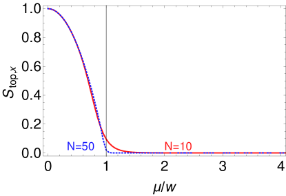
Figure 2: String order parameter $S_{\mathrm{top},x}$ for $N=10$ (red solid line) and $50$ (blue dotted line) topological superconducting wires as a function of the chemical potential $\mu$ in equilibrium at zero temperature. Here we set $w=\Delta=1$. The order parameter exhibits a second-order-type transition behavior: it is finite in the topological phase ($\mu<w$) and vanishes in the non-topological phase ($\mu>w$).

In general, the ferromagnetic ordering can arise along the spin-$y$ direction if the spin XY model ($J_{x},J_{y}\neq 0$) is taken into account or when the system evolves with time under the transverse magnetic field so that the spins precess. Specifically, the spin-$y$ correlation between two edge spins, $\mathinner{\langle{\textstyle\sigma_{1}^{y}\sigma_{N}^{y}}\rangle}$, is written via the Jordan-Wigner transformation as

$$S_{\mathrm{top},y}=\mathinner{\langle{\textstyle\gamma_{1}\left[\prod_{j=2}^{N-1}(-i\gamma_{2j-1}\gamma_{2j})\right](i\gamma_{2N})}\rangle}=(-1)^{N-1}\mathinner{\langle{\textstyle\prod_{j=1}^{N-1}(-i\gamma_{2j-1}\gamma_{2j+2})}\rangle}.$$ (6)

Interestingly, this string order parameter vanishes for the configuration in Fig. 1(b) but becomes one for that in Fig. 1(c). Therefore, the spin-$x$ and -$y$ correlations capture two different kinds of topological order for which the topological invariant is 1 or $-1$, respectively. Hence, the sum of two order parameters defines the total topological order:

$$S_{\mathrm{top}}=S_{\mathrm{top},x}+S_{\mathrm{top},y}$$ (7)

which is no other than the spin correlation $\mathinner{\langle{\textstyle\sigma_{1}^{x}\sigma_{N}^{x}+\sigma_{1}^{y}\sigma_{N}^{y}}\rangle}$ in the $xy$ plane perpendicular to the transverse field.

From the dynamical point of view, the most fascinating aspect of this string order parameter is that it is defined with respect to the wave function, not to the Hamiltonian. The so-called topological invariants which are commonly used to clarify the topological property of the system at equilibrium are basically the properties of the Hamiltonian. Therefore they are inadequate for the study of the evolution of the topological order triggered by the change of the Hamiltonian with time such as quench. Quite contrary, the string order parameter $S_{\mathrm{top}}$ is the expectation value of Majorana operators with respect to the wave function which evolves with time, so it can capture the dynamical evolution of the topological order in the wave function.

The string order parameters can be defined over a part of the chain as well as the whole. For later use, we define the string order parameters for the region from site $j_{1}$ to $j_{2}$ as

$$S_{\mathrm{top},x}(j_{1},j_{2}) =\mathinner{\langle{\textstyle\prod_{j=j_{1}}^{j_{2}-1}(-i\gamma_{2j}\gamma_{2j+1})}\rangle}$$ (8a)

$$S_{\mathrm{top},y}(j_{1},j_{2}) =(-1)^{j_{2}-j_{1}}\mathinner{\langle{\textstyle\prod_{j=j_{1}}^{j_{2}-1}(-i\gamma_{2j-1}\gamma_{2j+2})}\rangle}$$ (8b)

$$S_{\mathrm{top}}(j_{1},j_{2}) =S_{\mathrm{top},x}(j_{1},j_{2})+S_{\mathrm{top},y}(j_{1},j_{2}).$$ (8c)

2.3 Time Evolution and Majorana Correlation Matrix

In order to calculate the string order parameter, we first introduce a $2N\times 2N$ skew-symmetric Majorana correlation matrix $C(t)$ whose elements are defined by

$$C_{kk^{\prime}}(t)=-i\left(\mathinner{\langle{\textstyle\gamma_{k}(t)\gamma_{k^{\prime}}(t)}\rangle}-\delta_{kk^{\prime}}\right)$$ (9)

for $k,k^{\prime}=1,\cdots,2N$. The Hamiltonian (1a) is quadratic and one can apply Wick’s theorem to evaluate the string order parameter. Wick’s theorem tells us that the expectation value of the products of $\gamma_{k}$ is the sum of all the possible products of the expectation values of pairs. The permutation between operators can change the overall sign if it happens in an odd number. The results can thus be expressed in terms of Pfaffian of the Majorana correlation matrix [37, 38]. More explicitly,

$$S_{\mathrm{top},x}(j_{1},j_{2})=\operatorname{Pf}[C^{(x)}(j_{1},j_{2})],\quad S_{\mathrm{top},y}(j_{1},j_{2})=-\operatorname{Pf}[C^{(y)}(j_{1},j_{2})],$$ (10)

where $C^{(x)}(j_{1},j_{2})$ and $C^{(y)}(j_{1},j_{2})$ are $2(j_{2}-j_{1})\times 2(j_{2}-j_{1})$ submatrices of $C$ formed by rows and columns $2j_{1},2j_{1}+1,\cdots,2j_{2}-2,2j_{2}-1$ and $2j_{1}-1,2j_{1}+1,2j_{1}+2,\cdots,2j_{2}-3,2j_{2}-2,2j_{2}$, respectively.

Now we formulate the time evolution of the correlation matrix $C(t)$. The Heisenberg equations of motion for the Majorana operators lead to the differential equation for $\widetilde{C}_{kk^{\prime}}(t)=\mathinner{\langle{\textstyle\gamma_{k}(t)\gamma_{k^{\prime}}(t)}\rangle}$:

$$i\hbar\frac{d\widetilde{C}(t)}{dt}=M(t)\widetilde{C}(t)-\widetilde{C}(t)M(t)$$ (11)

with

$$M(t)=i\left[\begin{array}[]{cccccccccc}0&-\mu_{1}&0&w_{-}&0&0&\cdots&0&0&0\\ \mu_{1}&0&w_{+}&0&0&0&\cdots&0&0&0\\ 0&-w_{+}&0&-\mu_{2}&0&w_{-}&\cdots&0&0&0\\ -w_{-}&0&\mu_{2}&0&w_{+}&0&\ddots&0&0&0\\ 0&0&0&-w_{+}&0&-\mu_{3}&\ddots&w_{-}&0&0\\ 0&0&-w_{-}&0&\mu_{3}&0&\ddots&0&0&0\\ \vdots&\vdots&\vdots&\ddots&\ddots&\ddots&\ddots&-\mu_{N{-}1}&0&w_{-}\\ 0&0&0&0&-w_{-}&0&\mu_{N{-}1}&0&w_{+}&0\\ 0&0&0&0&0&0&0&-w_{+}&0&-\mu_{N}\\ 0&0&0&0&0&0&-w_{-}&0&\mu_{N}&0\end{array}\right]$$ (12)

and

$$w_{\pm}\equiv\frac{\Delta\pm w}{2}.$$ (13)

By solving the differential equation, we obtain

$$\widetilde{C}(t)=U(t)\widetilde{C}(0)U^{t}(t)$$ (14)

with the time evolution matrix

$$U(t)=T\exp\left[-\frac{i}{\hbar}\int_{0}^{t}d\tau\,M(\tau)\right].$$ (15)

Finally,

$$C(t)=(-i)(\widetilde{C}(t)-1)=(-i)(U(t)\widetilde{C}(0)U^{t}(t)-1)=U(t)C(0)U^{t}(t)$$ (16)

since $U(t)$ is orthogonal matrix. Note that if $C(0)$ is real, the $C(t)$ is real for all time $t$.

2.4 General Structure of Majorana Correlation Matrix

In general, the wave functions of the two Majorana edge states overlap with each other, giving rise to a finite energy splitting (although exponentially small for a long chain). So the ground state has a definite fermion parity: In our study we choose $P=1$. Note that the fermion parity, Eq. (2), is no other than the Pfaffian of $C$: $P=\operatorname{Pf}[C]$. Therefore, $\operatorname{Pf}[C]=1$ throughout the time evolution. On the other hand, the real $2N\times 2N$ skew-symmetric matrix can be always block-diagonalized by an orthogonal matrix $V$: $C=VDV^{t}$ with

$$D=\bigoplus_{n=1}^{N}\begin{bmatrix}0&\lambda_{n}\\ -\lambda_{n}&0\end{bmatrix}$$ (17)

where $\lambda_{n}$ are real. Since $\operatorname{Pf}[C]=\det[V]\,\operatorname{Pf}[D]=\operatorname{Pf}[D]=\prod_{n=1}^{N}\lambda_{n}=1$ and the correlation between the Majorana operators cannot be larger than 1 in magnitude, one can conclude that $\lambda_{n}=1$ for all $n$. It leads to an interesting physical implication: In a proper basis, each of $2N$ Majorana fermions forms a pair with another single Majorana fermion (not a superposition of pairs with different Majorana fermions), resulting in $N$ definite pairs. The simplest examples are shown in Figs. 1(b) and (c); with the fermion parity fixed, two edge Majorana fermions, isolated otherwise, should form a non-local pair. It is stressed that for a general dynamical wavefunction the Majorana fermions are not necessarily localized at one site as in Figs. 1(b) and (c), but they can move along the wire or disperse with time. Such propagation and spread of each Majorana fermion are reflected in the time evolution matrix $U(t)$. In other words, by tracking down the time evolution of each column of $U(t)$, one can find that which Majorana fermion forms a pair with which Majorana fermion at each time. Importantly, this information in turn can be used to interpret the dynamical change of $S_{\mathrm{top}}$ with time. For example, $S_{\mathrm{top},x}(j_{1},j_{2})$ would be maximal when the Majorana fermions $\gamma_{2j_{1}},\gamma_{2j_{1}+1},\cdots,\gamma_{2j_{2}-2},\gamma_{2j_{2}-1}$ strongly form pairs by themselves. If any of them is bound to that outside the region, then the topological order in that region must decrease.

2.5 Quench Dynamics

Throughout the study, for simplicity, we take the Ising limit in which the $p$-wave superconducting order parameter $\Delta$ is equal to the hopping amplitude $w$: $w_{+}=w$ and $w_{-}=0$. The Ising case can reveal the key essence of the dynamics of the topological order. Since we are interested in the quench dynamics of the system, the parameters of the system are driven to change in time. Taking into account the feasibility of experimental realization, the hopping amplitude as well as the superconducting gap is fixed in time and position-independent, while the position-dependent chemical potential $\mu_{j}(t)$, which can be easily controlled experimentally, is varied with time so that the whole or a part of the system experience dynamical topological phase transition.

In our study we consider two cases: In the first case, the wire is uniform so that $\mu_{j}(t)=\mu(t)$ and a quantum quench is applied at time $t=0$

$$\mu(t)=\begin{cases}0,&t<0\\ \mu_{f},&t>0\end{cases}$$ (18)

so that the whole wire is driven from the deep topological phase ($\mu=0$) to the non-topological phase ($\mu=\mu_{f}>w$). In the second case, only the central region with $N_{\mathrm{sys}}$ sites (called as the system) is initially prepared in the topological phase ($\mu_{j}=\mu_{\mathrm{sys}}=0$) and the side regions (called as the environment) with $N_{\mathrm{env}}\equiv(N-N_{\mathrm{sys}})/2$ sites in each side are in the non-topological phase ($\mu_{j}=\mu_{\mathrm{env}}>w$). At time $t=0$, the system part is driven to the non-topological phase like in the environment:

$$\mu_{\mathrm{sys}}(t)=\begin{cases}0,&t<0\\ \mu_{f},&t>0\end{cases}\quad\text{and}\quad\mu_{\mathrm{env}}(t)=\mu_{f}.$$ (19)

For convenience, we set $\hbar=1$ and focus on the zero temperature case.

3 Time Evolution of Topological Order in Uniform Wire

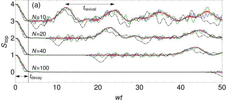
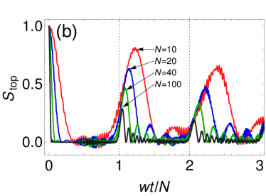
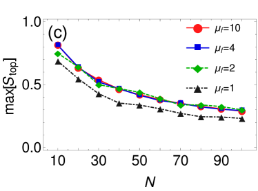
Figure 3: (a) Time evolution of string order parameter $S_{\mathrm{top}}$ for topological superconducting wires with different lengths after the quench, Eq. (18), for several values for $\mu_{f}/w$: 10 (red solid), 4 (green dotted), 2 (blue dashed), and 1 (black dot-dashed), (b) Time-scaled version of the time evolution for $\mu_{f}/w=10$, and (c) the maximum amplitude of $S_{\mathrm{top}}$ at the first revival as a function of the wire length $N$. Note that the curves for different system size $N$ in figure (a) are shifted by one. Here we set $w=\Delta=1$.

In this section we consider the quantum quench of a uniform $p$-wave superconducting wire from the topological to non-topological phase according to Eq. (18). Figure 3 displays the time evolution of $S_{\mathrm{top}}$ after the quantum quench at $t=0$. Here we summarize the two characteristic behaviors of the string order parameter uncovered in Fig. 3 (and below we explain them in terms of the motion of Majorana fermions): (i) The topological orders defined by Eqs. (5), (6), and (7) do not die away immediately after the quench, but instead decay with time before they vanish completely. Interestingly, the shape of $S_{\mathrm{top}}(t)$ during the decay and the decaying time $t_{\mathrm{decay}}$ are quite universal: As long as $\mu_{f}$ is not too close to the transition point $w$, we numerically find $wt_{\mathrm{decay}}\approx\pi$, which is immune to the wire length $N$ and the final value of the chemical potential $\mu_{f}$. This size-independence is quite interesting considering that the topological order is based on the nonlocal products of operators [see Eqs. (5) and (6)]. We also find that as long as $\mu_{f}>w$ the overall behavior of $S_{\mathrm{top}}$ is qualitatively same for all values of $\mu_{f}$, except additional small oscillations whose amplitude and period decrease with increasing $\mu_{f}$, as seen in Fig. 3(a). (ii) The topological order is revived repeatedly although the amplitude gradually decreases. Specifically, the topological order reappears at $t\approx nN/w$ ($n=1,2,\cdots$) and is kept for a duration time which is around $2t_{\mathrm{decay}}$, forming peaks centered at $t\approx nN/w+t_{\mathrm{decay}}$, as seen in Figs. 3(a) and (b). The revival period, the time between the peaks in $S_{\mathrm{top}}(t)$, is definitely related to the system size: $t_{\mathrm{revival}}\sim N/w$. Surely, the revival is the finite-size effect. Figure 3(c) shows that the maximum amplitude of $S_{\mathrm{top}}$ at its first revival decreases with the system size and that its dependence on $N$ is immune to the quench strength as long as $\mu_{f}$ is sufficiently larger than $w$. This observation can be explained in terms of the dispersion of the Majorana wave function, which will be discussed in greater detail later. Note that a similar kind of revival of Majorana physics has been reported by examining the survival probability of edge Majorana states in the same system [17]. In their study the survival of local Majorana wave function is maximal in the quench to the transition point ($\mu_{f}=w$). However, the revival of non-local topological order in our study turns out to be quite robust no mater what value $\mu_{f}$ has.

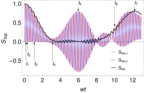
Figure 4: Time evolution of string order parameters $S_{\mathrm{top},x/y}$ and $S_{\mathrm{top}}$ for $N=10$ topological superconducting wires after the quench, Eq. (18) with $\mu_{f}/w=10$.

In passing, we examine and compare the time evolutions of different string order parameters, $S_{\mathrm{top},x/y}$ as well as $S_{\mathrm{top}}$, more closely. Figure 4 shows that unlike $S_{\mathrm{top}}$ the string order parameters $S_{\mathrm{top},x/y}$ oscillate rapidly in the anti-synchronized way. The initial oscillation with $\pi/2$ phase difference between $S_{\mathrm{top},x/y}$ can be understood in the spin language. Initially, the ferromagnetic coupling $J_{x}=w/2$ aligns all the spins in the $x$ direction. Turning on the transverse magnetic field $h_{z}$ makes the spins precess in the $xy$ plane, transferring the correlation in the $x$ direction into that in the $y$ direction and vice versa. The spin precession under the transverse field is responsible for the oscillation whose period is then inversely proportional to $1/|h_{z}|\propto 1/\mu_{f}$.

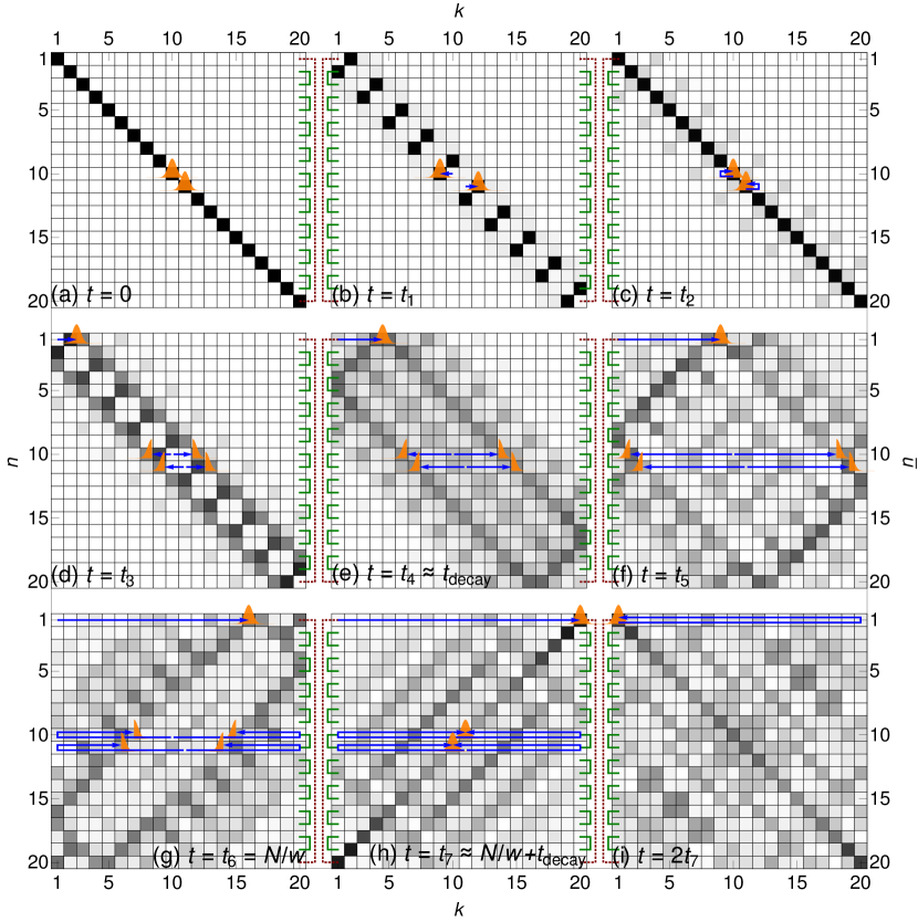
Figure 5: Density plot of the time evolution matrix $|U_{kn}|$ for the time evolution of $N=10$ topological superconducting wires after the quench, Eq. (18) with $\mu_{f}/w=10$. The times at which the matrix elements are taken are indicated in Fig. 3: (a) $t=0$, (b) $t=t_{1}$ when $S_{\mathrm{top},x}=0$ for the first time, (c) $t=t_{2}$ when $S_{\mathrm{top},y}=0$ for the second time, (d) $t=t_{3}$ when $S_{\mathrm{top},x}=0$, (e) $t=t_{4}\approx t_{\mathrm{decay}}$ when $S_{\mathrm{top}}$ vanishes almost, (f) $t=t_{5}$ when the oscillation of $S_{\mathrm{top},x/y}$ is maximal again, (g) $t=t_{6}=N/w$, (h) $t=t_{7}\approx N/w+t_{\mathrm{decay}}$ when $S_{\mathrm{top}}$ is fully restored, and (i) $t=2t_{7}$. The green and red lines connecting rows indicates the pairing between the pairs of Majorana states.

All those aspects of the change of the string order parameter with time can be explained in terms of the time evolution of Majorana wave function reflected in the matrix $U(t)$, as we discuss in the remaining of the section. Figure 5 displays the time evolution of Majorana wave function: Each row of the density plots corresponds to the wave function of the Majorana state ordered in such a way that at $t=0$ the $n^{\mathrm{th}}$ state ($1\leq n\leq 2N$) is localized at Majorana site $k=n$. Hence, according to the initial pairing between Majorana fermions depicted in Fig. 1(b), the $n=2j$ and $2j+1$ Majorana states ($j=1,2,\cdots,N-1$) are paired and the edge Majorana states ($n=1$ and $2N$) are also paired due to the fermion parity fixing [see the green and red lines in Fig. 5(a)]. While the wave functions of the Majorana states change with time, theses pairings are maintained throughout the time evolution. Turning on the chemical potential couples $\gamma_{2j-1}$ and $\gamma_{2j}$ so that the Majorana fermions hop between two Majorana sites in a real site $j$. At $t=t_{1}\approx\pi/2\mu_{f}$, the Majorana fermions in a real site exchange between them [see Fig. 5(b)] so that the Majorana configuration is almost same as Fig. 1(c), resulting in $S_{\mathrm{top},x}=0$ and $S_{\mathrm{top},y}\approx 1$. At $t=t_{2}\approx\pi/\mu_{f}$, the Majorana fermions return to their starting points [see Fig. 5(c)], restoring $S_{\mathrm{top},x}\approx 1$ almost with $S_{\mathrm{top},y}=0$.

The oscillation is accompanied with the dispersion of the Majorana states, making the pairing between the bulk and edge Majorana states gradually increasing and accordingly weakening $S_{\mathrm{top}}$. On top of it, each Majorana wave function (except $n=1,2N$ Majorana states) is split into two propagation modes, moving in opposite directions [see Figs. 5(d) and (e)]. At $t=t_{4}\approx\pi/w$ [see Fig. 5(e)], the initial edge Majorana states ($n=1,2N$) enter into the bulk completely, and the propagation of split Majorana states, initially starting in the bulk, hits the ends of the chain so that the correlation between the bulk and edge Majorana fermions becomes maximal, resulting in the vanishing of $S_{\mathrm{top},x/y}$ and $S_{\mathrm{top}}$. Since the decaying of the topological order happens when the initial edge Majorana states enter into the bulk, the decaying time does not depend on the system size. Also, noting that the propagation speed of the Majorana states is mainly determined by the hopping amplitude $w$, the chemical potential strength does not affect the decaying time $t_{\mathrm{decay}}$.

For $t\lesssim N/w$, the topological order parameters $S_{\mathrm{top}}$ and $S_{\mathrm{top},x/y}$ remain being suppressed except around $t\sim N/2w$ in which $S_{\mathrm{top},x}$ and $S_{\mathrm{top},y}$ oscillate out of phase. A typical distribution of Majorana states in that period is shown in Fig. 5(f). One can see that the Majorana states for $n=8\sim 13$ become mostly localized at the boundaries and form pairs by themselves: $\gamma_{1}$ and $\gamma_{2N}$, and $\gamma_{2}$ and $\gamma_{2N-1}$, simultaneously. The other Majorana states inside the bulk are binding by themselves as well. It satisfies the condition to have finite $S_{\mathrm{top},x/y}$ as shown in Fig. 4. Note that the pairing inside the bulk is not like those in Fig. 1(b) nor (c), where the Majorana fermions in neighboring sites form pairs, but instead is more like that in Fig. 1(a), where the Majorana fermions in the same site is bound. Hence, it results in the almost perfect cancellation between $S_{\mathrm{top},x}$ and $S_{\mathrm{top},y}$, making $S_{\mathrm{top}}$ vanish. In this respect, $S_{\mathrm{top}}$, not $S_{\mathrm{top},x}$ nor $S_{\mathrm{top},y}$, is the more adequate order parameter to measure the topological order.

At $t=t_{6}=N/w$ [see Fig. 5(g)], the front part of the initial edge Majorana wave function $(n=1,2N)$ starts to reach the opposite ends, and the bulk Majorana states which was split becomes reunited. That is, apart from the dispersion of Majorana states, the Majorana configuration starts to be restored to the initial one with reverse ordering, which accordingly revives the topological order. At $t=t_{7}\approx N/w+t_{\mathrm{decay}}$ [see Fig. 5(h)], the topological order is maximally restored, restoring the initial Majorana configuration. Note that while the bulk states are considerably dispersed, the Majorana states for $n=1,2N$, forming a strong pair, are still quite localized at the edges. This is the reason why the restoration of $S_{\mathrm{top}}$ is quite strong. Finally, at $t=2t_{7}\approx 2N/w$ [see Fig. 5(i)], the Majorana configuration returns to the initial one with much dispersion, leading to the second revival of the topological order. Note that our analysis which tracks down the pairing between Majorana states explains why the revival period of the topological order is $N/w$, the half of the round-trip period ($=2N/w$) of Majorana states.

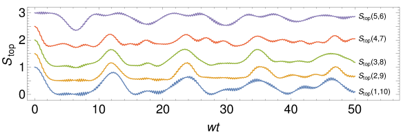
Figure 6: Time evolution of string order parameter $S_{\mathrm{top}}(j_{1},j_{2})$ for $N=10$ topological superconducting wires after the quench, Eq. (18) with $\mu_{f}/w=10$. Each curve is shifted by 1/2.

Now we examine the time evolution of $S_{\mathrm{top}}(j_{1},j_{2})$ for central segments of the wire from site $j_{1}$ to site $j_{2}=N+1-j_{1}$. Figure 6 shows that the revival of the topological order happens for all $S_{\mathrm{top}}(j_{1},j_{2})$ simultaneously. It means that the pairing of Majorana fermions is like that in Figs. 1(b) or (c) in any length scale, once the order is restored. For the quench in uniform wires, this is the case as can be seen in Figs. 5(h) and (i).

Finally, we address interesting relations between the string order parameters $S_{\mathrm{top},x/y}$ and the elements of the correlation matrix $C$. From the observations up to now, it is obvious that $S_{\mathrm{top},x}$ increases as the Majorana fermions $\gamma_{k}$ on sites $k=2,\cdots,2N-1$ form strong pairs by themselves. Under the condition that the fermion parity is fixed, every Majorana fermion should be bound to one of others. Hence, with $S_{\mathrm{top},x}$ close to one by binding $\gamma_{k}$ for $k=2,\cdots,2N-1$, a strong pair between $\gamma_{1}$ and $\gamma_{2N}$ should be formed. It implies that $S_{\mathrm{top},x}$ and $C_{1,2N}$ are positively correlated. A similar argument also leads to a positive correlation between $S_{\mathrm{top},y}$ and $C_{2,2N-1}$. As proven in A, this kind of correlations is exact:

$$S_{\mathrm{top},x} =C_{1,2N}$$ (20a)

$$S_{\mathrm{top},y} =-C_{2,2N-1}$$ (20b)

[see Eqs. (33) and (34)]. Therefore, the topological order can be obtained simply from the correlations between edge Majorana fermions. This result may lead to a false understanding that the topological order is in fact local since $C_{1,2N}$ or $C_{2,2N-1}$ are local correlations. However, we can argue that the topological order is really nonlocal in two ways: (i) These relations, Eqs. (20a) and (20b) are based on the assumption that the fermion parity is fixed. However, as pointed out in Ref. [31], the string order parameter is insensitive to the linear combination of degenerate ground states with different parities. So even when the relations between the string order parameter and the edge Majorana correlation are not valid, the nonlocal string order parameter is still unambiguously defined. (ii) The derivation leading to Eqs. (20a) and (20b) states that the string order parameter over a part of the system is related to the correlation outside the part [see Eq. (35)]. Equations (20a) and (20b) are special cases where the remaining part consists of only two (edge) Majorana fermions. So the topological order is truly global property of the system, reflecting the correlations all over the system.

4 Propagation of Topological Order into Non-Topological Regions

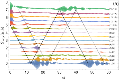
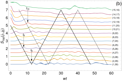
Figure 7: Time evolution of string order parameter (a) $S_{\mathrm{top},x}(j_{1},j_{2})$ and (b) $S_{\mathrm{top}}(j_{1},j_{2})$ for $N=30$ topological superconducting wires with $N_{\mathrm{sys}}=10$ central sites initially prepared in topological phase after the quench, Eq. (19) with $\mu_{f}/w=10$. Each curve is tagged with the corresponding site interval $(j_{1},j_{2}{=}N{+}1{-}j_{1})$ and is shifted by 1/2 for clarity. The solid and dotted lines are guide for Majorana fermion propagation which is explained in the text.

Now we consider the case in which only a central part (“system” with $N_{\mathrm{sys}}$ sites) of the superconducting wire is initially in topological phase and the outer part (“environment” with $N_{\mathrm{env}}$ sites on the left and another $N_{\mathrm{env}}$ sites on the right) is in non-topological phase, according to Eq. (19). Figure 7 shows the time evolution of $S_{\mathrm{top},x}(j_{1},j_{2})$ and $S_{\mathrm{top}}(j_{1},j_{2})$ for every (centered) region (we take $j_{1}$ and $j_{2}$ symmetrically so that $j_{2}=N+1-j_{1}$) of the wire with $N=30$ and $N_{\mathrm{sys}}=10$ (accordingly, $N_{\mathrm{env}}=10$) after a sudden quench. At $t=0$, the system part is in topological phase so that $S_{\mathrm{top},x}(j_{1},j_{2})=S_{\mathrm{top}}(j_{1},j_{2})=1$ for $N_{\mathrm{env}}<j_{1}\leq N/2$. However, the string order parameters for larger regions which extend into the environment part are initially zero: $S_{\mathrm{top},x}(j_{1},j_{2})=0$ for $j_{1}\leq N_{\mathrm{env}}$ since $\gamma_{2j_{1}}$ at site $j_{1}$ in the environment region form a strong pair with $\gamma_{2j_{1}-1}$ which is not included in the string of Majorana operators $\gamma_{2j_{1}}\gamma_{2j_{1}+1}\cdots\gamma_{2j_{2}-1}$ for $S_{\mathrm{top},x}(j_{1},j_{2})$ [see Eq. (8a)].

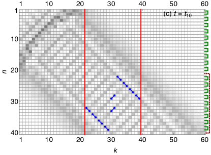
Figure 8: Density plot of the time evolution matrix $|U_{kn}|$ for the time evolution of $N=30$ and $N_{\mathrm{sys}}=10$ topological superconducting wires initially prepared as described in Fig. 7. The times at which the matrix elements are taken are indicated in Fig. 7: (a) $t=t_{8}$ when $S_{\mathrm{top}}(5,26)$ becomes maximal for the first time, (b) $t=t_{9}$ when $S_{\mathrm{top}}(1,30)$ becomes maximal for the first time, and (c) $t=t_{10}$ when $S_{\mathrm{top}}(11,20)$ is fully revived for the first time. In all cases, $S_{\mathrm{top},y}\approx 0$. The green and red lines connecting rows (in the right side of the figures) indicates the pairing between the pairs of Majorana states. The red vertical lines indicate the regions in which the topological order is measured. The blue small circles and (solid and dotted) lines connecting them pick the Majorana pairs which mostly contributes to the corresponding $S_{\mathrm{top},x}$.

After quench, $S_{\mathrm{top},x}(j_{1},j_{2})$ and $S_{\mathrm{top}}(j_{1},j_{2})$ in the system part decays with time, which is almost similar to the decay behavior observed in the uniform case [compare with Fig. 6]. However, very interestingly, the topological order parameters for larger region, which are initially zero, become finite after some time passes [follow the solid and dotted lines in Fig. 8]. We find that the time for $S_{\mathrm{top}}(j_{1},j_{2})$ with $j_{1}\leq N_{\mathrm{env}}$ to be maximally increased is approximately $(N_{\mathrm{env}}+1-j_{1})/w$: For example, the time when $S_{\mathrm{top}}(1,N)$ becomes maximal is around $N_{\mathrm{env}}/w$. These findings strongly suggest that the topological order propagates into the non-topological region with a constant velocity after the quench.

The mechanism for the propagation of the topological order can be understood in terms of the time evolution of Majorana wave functions, as in the uniform case. Figure 8(a) shows the snapshot of Majorana wave function at $t=t_{8}$ when $S_{\mathrm{top}}(j_{1},j_{2})$ for $j_{1}=5$ is maximal with $S_{\mathrm{top},x}(j_{1},j_{2})\approx S_{\mathrm{top}}(j_{1},j_{2})$ and $S_{\mathrm{top},y}(j_{1},j_{2})\approx 0$ as marked in Fig. 7(b). The Majorana fermions which are initially inside the system part and form the topological pairing are split and propagate into either direction. At $t=t_{8}$, the main part of the Majorana wave functions covers the whole region of Majorana sites for $S_{\mathrm{top}}(j_{1},j_{2})$ with $j_{1}=5$ as marked by red vertical lines in Fig. 8(a). It clearly reveals that the propagation of the topological order is connected to that of the Majorana wave functions, which determines the propagation speed. The blue circles and lines connecting them in the figure pick some of the Majorana pairings which make finite contribution to $S_{\mathrm{top},x}$ and $S_{\mathrm{top}}$. Moreover, since the Majorana wave function has been spatially split, the pairing of Majorana fermions contributing to the topological order is now nonlocal: The Majorana fermions are bound not only to the nearest neighboring one but also to that moving in the opposite direction with increasing distance between them (see the connections with dotted lines). Note that this nonlocal pairing leads to the vanishing of $S_{\mathrm{top}}(j^{\prime}_{1},j^{\prime}_{2})$ for almost all $j^{\prime}_{1}>j_{1}$: While the topological order arises in the region $(j_{1},j_{2})$ for $j_{1}=5$ at $t=t_{8}$, it does not for smaller region. The reason is that the pairing of Majorana fermions inside the smaller region is not closed by themselves due to the nonlocal pairing. Some of Majorana fermions are bound to those outside the region. It is quite different from the uniform case in which the topological order is revived in all scales. On the other hand, we would like to point out that even when $S_{\mathrm{top}}(j_{1},j_{2})$ is maximal its value is rather small: For example, $S_{\mathrm{top}}(j_{1},j_{2})\approx 0.2$ for $j_{1}=5$. It is because the non-topological pairing of Majorana fermions starting from the environment part is also propagating into that region $(j_{1},j_{2})$.

The topological order eventually covers the whole wire, which occurs at $t=t_{9}$ as seen in Fig. 7. At this time, the Majorana fermions forming the topological pairing reach their outermost boundaries which are $k=2$ and $2N-1$ for $S_{\mathrm{top},x}$ [see the red vertical lines in Fig. 8(b)]. So, although not perfect, the Majorana pairings become similar to those in Fig. 1(b) with additional nonlocal pairings. After $t=t_{9}$, the Majorana fermions maintaining the topological pairing are reflected at the boundaries and some of them going inside the wire so that the region having the topological order shrinks (follow the solid lines in Fig. 7). As the Majorana wave functions propagate, the topological region should repeat expanding and shrinking. However, the dispersion of the Majorana wave function causes topological order to gradually decay.

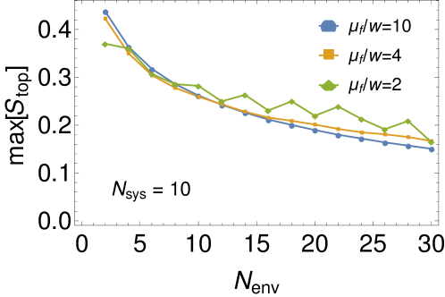
Figure 9: Maximum value of $S_{\mathrm{top}}$ when the topological order propagates over the entire wire at the first time as a function of $N_{\mathrm{env}}$ for different values of $\mu_{f}$. Here we use $N_{\mathrm{sys}}=10$.

While the topological region is determined mainly by the outermost boundaries of Majorana wave function with topological paring, the inner boundaries of Majorana fermions can also define the topological region. Figure 8(c) shows the Majorana wave function at $t=t_{10}$ when $S_{\mathrm{top}}(j_{1},j_{2})$ for the system part ($j_{1}=11$) is revived. While this revival is not due to the recombination of split Majorana wave function as happens in Fig. 5(g), it can be also explained in terms of the time evolution of Majorana wave functions. First, consider the initial edge Majorana fermions, $\gamma_{2\times 11-1}$ and $\gamma_{2\times 20}$ for the topological system part, connected by the red dotted line in Fig. 8. After the quench, they are split and the two parts of each of them move outward and inward, respectively. So after some time passes (around $t=t_{10}/2$) the inner parts of their split Majorana wave functions cross each other. After that, they define the boundaries of another topological region in which the topological pairing is significant as shown in Fig. 8(c). Such a revival of the topological order happens along the dotted lines in Fig. 7. Since the boundary of the topological region is moving with time, this topological order also propagates along the wire.

Since the propagation of the Majorana wave function is accompanied with its dispersion, the topological order when it covers the whole wire should be weaker for longer wires. Figure 9 clearly confirms this expectation: $S_{\mathrm{top}}$ at its first maximum decreases monotonically with increasing $N_{\mathrm{env}}$, except small additional oscillations observed for $\mu_{f}$ close to $w$. It shows that as long as $\mu_{f}$ is large enough the value of $\mu_{f}$ does not affect the propagation of the topological order as observed in the uniform case [compare with Fig. 3(c)].

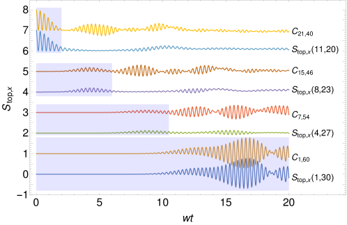
Figure 10: Comparison between the time evolution of $S_{\mathrm{top},x}(j_{1},j_{2})$ and $C_{2j_{1}-1,2j_{2}}$ for the quench used in Fig. 7. The shaded boxes mark the time interval in which those two quantities are in perfect or good agreement with each other.

In the previous section, we observed interesting relations between the string order parameters and the elements of the Majorana correlation matrix, such as Eqs. (20a) and (20b), for the uniform wire. Here we demonstrate that similar relations hold in the non-uniform case as well. First, as seen in Fig. 10, the nonlocal topological order for the whole system, $S_{\mathrm{top},x}=S_{\mathrm{top},x}(1,2N)$ is exactly equal to the correlation $C_{1,2N}$ between Majorana fermions at the ends of wire, which in fact comes from the exact identity, see Eq. (20a). Then, one may question if a similar relation such as $S_{\mathrm{top},x}(j_{1},j_{2})=C_{2j_{1}-1,2j_{2}}$ can hold for a part of the system. As shown in A, there is no such equation identity. However, Fig. 10 demonstrates that the relation can be valid at least for a finite time after the quench. The temporary agreement between $S_{\mathrm{top},x}(j_{1},j_{2})$ and $C_{2j_{1}-1,2j_{2}}$ can be understood in terms of the general relation, Eq. (35). Until the topological order spreads over the region $(j_{1},j_{2})$, one can assume that the outer region remains strictly in the non-topological phase so that the Majorana fermions in that region form the non-topological pairings like in Fig. 1(a) and the string order parameters $\mathinner{\langle{\textstyle\prod_{j=1}^{j_{1}-1}(-i\gamma_{2j-1}\gamma_{2j})}\rangle}$ and $\mathinner{\langle{\textstyle\prod_{j=j_{2}-1}^{N}(-i\gamma_{2j-1}\gamma_{2j})}\rangle}$ for the left- and right-side environments are one. Therefore, together with Eq. (35), we obtain

$$S_{\mathrm{top},x}(j_{1},j_{2})=\operatorname{Pf}[C_{\bar{\mathcal{J}},\bar{\mathcal{J}}}]=C_{2j_{1}-1,2j_{2}}$$ (21)

since only $\gamma_{2j_{1}-1}$ and $\gamma_{2j_{2}}$ in $\bar{\mathcal{J}}$ are not forming the non-topological pairing. The assumption leading to Eq. (21) is broken once the topological order spreads beyond the region $(j_{1},j_{2})$.

5 Experimental Detection of Topological Order

While from the theoretical point of view the notion of the topological order is interesting and useful in understanding new quantum states of matter, its direct measurement is highly non-trivial even at the conceptual level since it is a nonlocal property. In this respect, the existence of the string order parameter is encouraging because (although nonlocal) it is suitable with current technology for experimental measurement [28].

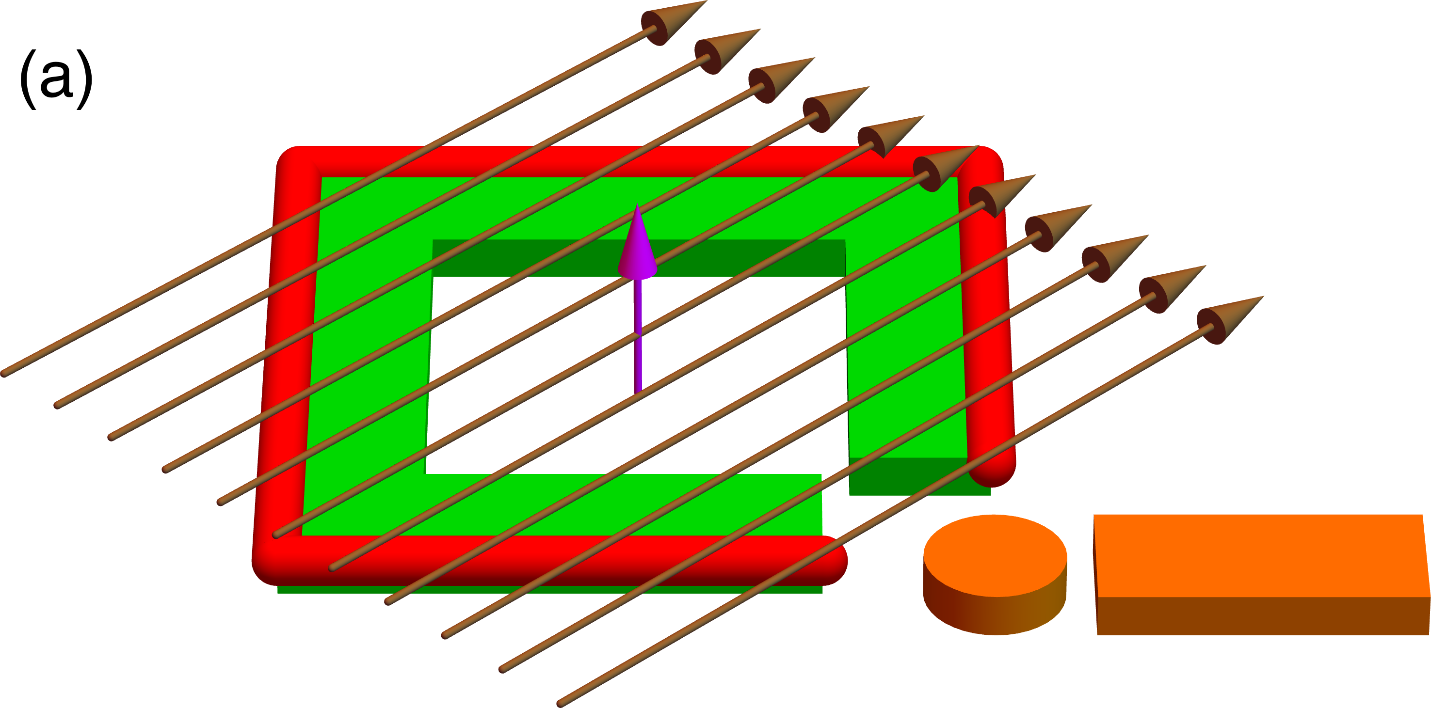
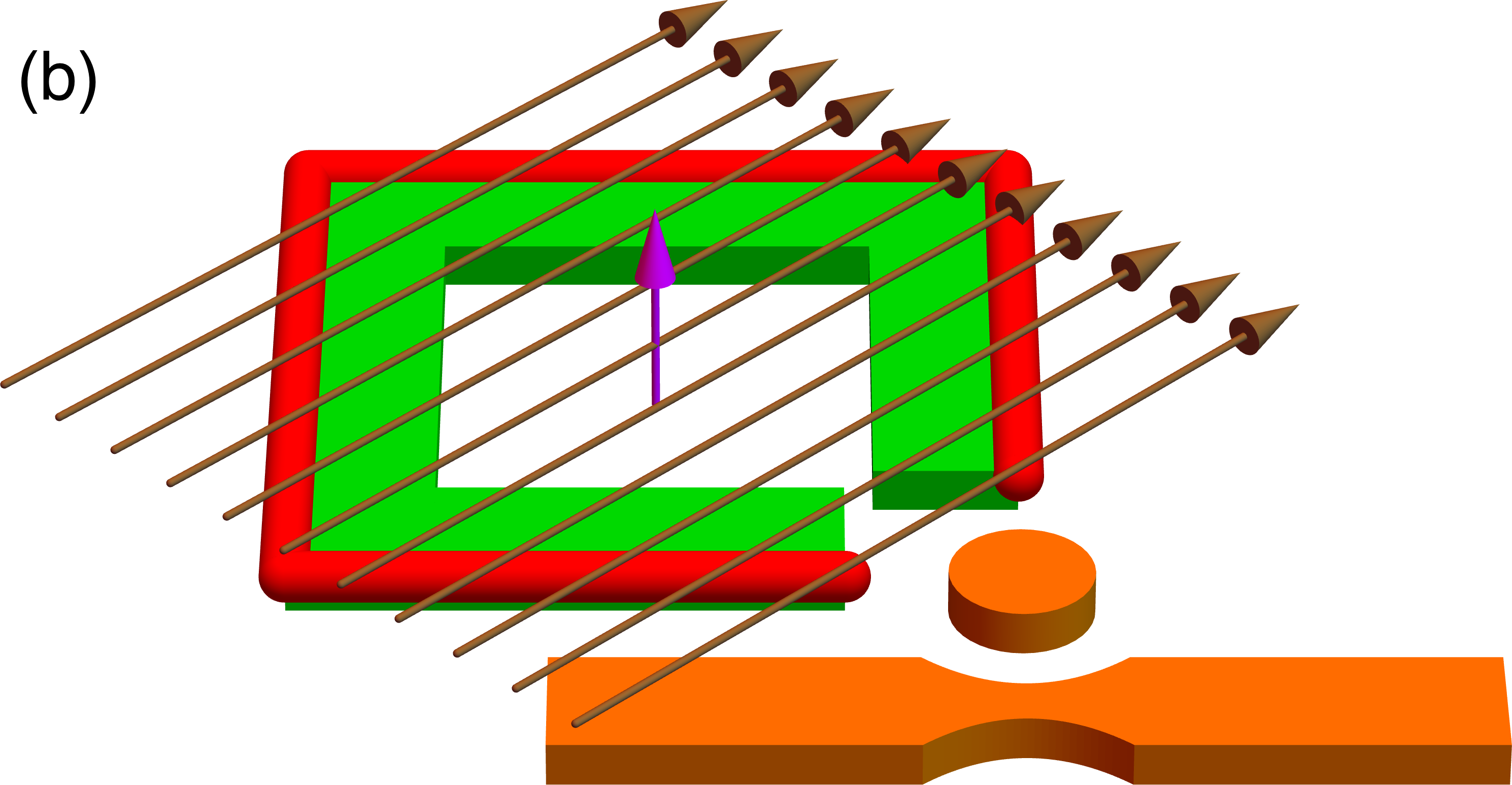
Figure 11: (color online) Two schemes for measuring the occupancy of the hybridized states, $c_{\pm}=(c_{1}\pm c_{N})/\sqrt{2}$, between the two end-site electrons $c_{1}$ and $c_{N}$. The wire (red) in the proximity to the conventional superconductor (green) and under the inplane magnetic field (black arrows) forms the topological superconductor. The two end-sites $c_{1}$ and $c_{N}$ are coupled to a quantum dot (orange disc). Depending on the additional flux $\Phi$ (brown arrow at the center) through the loop, either $c_{+}$ ($\Phi/\Phi_{0}=0$) or $c_{-}$ ($\Phi/\Phi_{0}=\pi$) electron can tunnel to the quantum dot. (a) The excess electron on the quantum dot is probed by taking it out to an additional normal lead (orange bar) attached to the dot. (b) The excess electron is probed by continuously monitoring the current through the nearby quantum point contact (orange pinched bar).

Here we propose a local and direct experimental way to probe the topological order. It is based on the relations between the string order parameters $S_{\mathrm{top},x/y}$ and the elements of the correlation matrix $C$ [see Eqs. (20a) and (20b)] discussed in Sections 3 and 4. First, note that the relations (20a) and (20b) allows us to rewrite the string order parameter $S_{\mathrm{top}}$ into

$$S_{\mathrm{top}}=C_{1,2N}-C_{2,2N-1}=-2\mathinner{\langle{\textstyle c_{1}^{\dagger}c_{N}+c_{N}^{\dagger}c_{1}}\rangle}=2(\mathinner{\langle{\textstyle c_{-}^{\dagger}c_{-}}\rangle}-\mathinner{\langle{\textstyle c_{+}^{\dagger}c_{+}}\rangle})$$ (22)

where $c_{\pm}=(c_{1}\pm c_{N})/\sqrt{2}$ are the fermion operators on the hybridized fermionic states between two end sites. Therefore, the string order parameter can be measured by probing the occupancy of the hybridized state $c_{\pm}$ between the two end-site electrons $c_{1}$ and $c_{N}$.

Figure 11 shows the schematics of two experimental setups to probe the hybridized states $c_{\pm}$. The quantum dot (the orange disc in Fig. 11) is tunnel coupled to the end sites $1$ and $N$ of the topological superconducting wire. It is described by the Hamiltonian of the standard form

$$H_{\text{probe}}=-w_{p}\,d^{\dagger}\left(e^{i\Phi/\Phi_{0}}c_{1}+c_{N}\right)+h.c.\,,$$ (23)

where $w_{p}$ is the coupling strength (assumed to be the same for $c_{1}$ and $c_{N}$ for simplicity), $d$ and $d^{\dagger}$ are quantum dot electron operators, $\Phi$ is the additional flux through the loop (the brown arrow in Fig. 11) formed by the wire and the quantum dot, and $\Phi_{0}=h/e$ is the magnetic flux quantum. When $\Phi/\Phi_{0}=0$, the hybridized electron $c_{+}$ ($c_{-}$) can (cannot) tunnel onto the quantum dot because of the constructive (destructive) interference. For $\Phi/\Phi_{0}=\pi$, it is the other way around. Therefore, by monitoring the excess electrons on the quantum dot, one can selectively detect the occupancies $\mathinner{\langle{\textstyle c_{\pm}^{\dagger}c_{\pm}}\rangle}$.

To monitor the excess charge on the quantum dot, there are several schemes available in the present state-of-the-art technology. Here we consider two different schemes. The first scheme [Fig. 11 (a)] is, in spirit, the same as the quantum optical method of detecting the occupancy of excited atomic levels by observing the emitted photons [39] as no photon is emitted by a ground-state atom. Operationally, it is similar to the on-demand single-electron emitter [40, 41, 42]: An excess electron on the dot is taken out to an additional normal lead $L$ attached to the dot by temporally manipulating the dot energy level $\epsilon_{d}(t)$. The dot-lead coupling is characterized by the level-broadening parameter $\Gamma_{L}$. Throughout the measurement procedure, a bias voltage is applied so that $\mu_{L}<\mu$, where $\mu_{L}$ and $\mu$ are the chemical potentials of the normal lead and the system, respectively. Initially, $\epsilon_{d}$ is set higher than $\mu$ so that no electron can tunnel into the quantum dot. At the desired moment of measurement, $\epsilon_{d}$ is lowered and tuned between $\mu_{L}$ and $\mu$ ($\mu_{L}<\epsilon_{d}<\mu$). The electron (if any) occupying the hybridized state $c_{\pm}$ will tunnel into the quantum dot and then to the normal lead. After a certain period $\tau_{p}$ of time, $\epsilon_{d}$ is pushed back higher than $\mu$. This procedure is repeated with interval $\tau_{r}$ ($1/\tau_{r}$ is typically in the GHz range [40, 41, 42]) many times enough for the electric current resolution. When the system is in the topological state, the Majorana states at the ends of the wire are expected to be true bound states, the current is estimated to be

$$I_{\pm}\approx\frac{4w_{p}^{2}\Gamma_{L}\tau_{p}}{\epsilon_{d}^{2}+4w_{p}^{2}}\frac{e}{\tau_{r}}\quad(w_{p}\ll\Gamma_{L})$$ (24)

if the hybridized state $c_{\pm}$ is occupied; the current vanishes otherwise.

In the second scheme [Fig. 11 (b)], the excess electron on the quantum dot is probed by continuously monitoring the current through a nearby quantum point contact [43, 44, 46, 47]. It is possible because the dot electron casts an additional Coulomb potential and reduces the transmission probability from $T_{\text{QPC}}$ to $T_{\text{QPC}}^{\prime}$ (hence the current from $I_{\text{QPC}}$ to $I_{\text{QPC}}^{\prime}$) through the quantum point contact. The change in the current is given by

$$I_{\text{QPC}}-I_{\text{QPC}}^{\prime}=\frac{e^{2}}{h}(T_{\text{QPC}}-T_{\text{QPC}}^{\prime})V_{\text{QPC}}\,,$$ (25)

where $V_{\text{QPC}}$ is the voltage bias applied across the quantum point contact. Note that the continuous monitoring affects the tunneling between the hybridized state $c_{\pm}$ and the dot. For example, when the system is in the topological state, the coherent oscillation of frequency $\sqrt{\epsilon_{d}^{2}+4w_{p}^{2}}$ between $c_{\pm}$ and $d$ is subject to the dephasing of rate $\Gamma_{\phi}\equiv\left(\sqrt{T_{\text{QPC}}}-\sqrt{T_{\text{QPC}}}^{\prime}\right)^{2}$ and the gradual relaxation of rate

$$\Gamma_{\text{mix}}=\frac{4w_{p}^{2}\Gamma_{\phi}}{\epsilon_{d}^{2}+\Gamma_{\phi}^{2}}$$ (26)

if the hybridized state $c_{\pm}$ is initially occupied; the oscillation is missing otherwise. The quantum point contact is often replaced with a single-electron transistor [48, 49, 50]. In either case, the change in charge on the quantum dot can be monitored as fast as the radio-frequency range. More detailed analyses including the effects of back-action noise are referred to Ref. [51] and references therein.

6 Conclusion

We have considered a wire of topological superconductor and studied the temporal evolution of the topological order upon a quantum quench across the critical point in terms of the string order parameter. Unlike topological quantum numbers, which are commonly used to describe the equilibrium topological order, the string order parameter is defined with respect to the full dynamical wave function and naturally captures the dynamical evolution of the topological order reflected in the wave function. It is considered to be more suitable for experimental observations [28]. We have found that the topological orders vanish with a finite decaying time and that the initial decaying behavior is universal in the sense that it does not depend on the wire length and the final value of the chemical potential (the quenching parameter). The revival of the topological order in finite-size wires and the propagation of the topological order into the region which was initially in the non-topological state have been observed and explained in terms of the propagation and dispersion of the Majorana wave functions. Finally, we have found the exact relations between the string order parameters and some local correlations, which are valid as long as the fermion parity is well defined. Based on these relations we have proposed a local probing method which allows to measure the topological order which is supposed to be nonlocal.

Appendix A Majorana Correlation Matrix and Topological Order

In this appendix we prove that the string order parameter over a part of the system is ultimately related to the correlation outside of that region and find the exact relation between them.

The Majorana correlation matrix $C(t)$ defined in Eq. (9) has the following properties as stated in the main text:

1. It is $2N\times 2N$ real skew-symmetric matrix.

2. $\operatorname{Pf}[C]=1$ due to the fixing of fermion parity.

3. It has eigenvalues of either $+i$ or $-i$. In other words, $C=VDV^{t}$ where $V$ is an orthogonal matrix and

   $$D=\bigoplus_{n=1}^{N}\begin{bmatrix}0&1\\ -1&0\end{bmatrix}.$$ (27)

From the property (iii), one can derive

$$C^{-1}=VD^{-1}V^{t}=V(-D)V^{t}=-C.$$ (28)

Now we recall the generalized Cramer’s rule [52]: For a nonsingular $n\times n$ matrix $A$ and $n\times m$ matrices $X$ and $B$ satisfying $AX=B$,

$$\det X_{{\mathcal{I}},{\mathcal{J}}}=\frac{\det A_{B}({\mathcal{I}},{\mathcal{J}})}{\det A},$$ (29)

where ${\mathcal{I}}=\{i_{1},i_{2},\cdots,i_{k}\}$ and ${\mathcal{J}}=\{j_{1},j_{2},\cdots,j_{k}\}$ are ordered sets of indices ($1\leq i_{1}\leq\cdots\leq i_{k}\leq n$ and $1\leq j_{1}\leq\cdots\leq j_{k}\leq m$), $X_{{\mathcal{I}},{\mathcal{J}}}$ is the $k\times k$ submatrix of $X$ with rows in ${\mathcal{I}}$ and columns in ${\mathcal{J}}$, and $A_{B}({\mathcal{I}},{\mathcal{J}})$ is the $n\times n$ matrix formed by replacing the $i_{s}^{\mathrm{th}}$ column of $A$ by the $j_{s}^{\mathrm{th}}$ column of $B$ for all $s=1,\cdots,k$.

In Eq. (29), we substitute $A=C$, $X=C^{-1}$, $B=1_{2N\times 2N}$, and ${\mathcal{J}}={\mathcal{I}}$. Then, the Cramer’s rule gives rise to

$$\det C^{-1}_{{\mathcal{I}},{\mathcal{I}}}=\frac{\det C_{\bar{\mathcal{I}},\bar{\mathcal{I}}}}{\det C}$$ (30)

since $\det A_{B}({\mathcal{I}},{\mathcal{I}})=\det C_{\bar{\mathcal{I}},\bar{\mathcal{I}}}$, where $\bar{\mathcal{I}}$ (also assumed to be ordered) is complementary to ${\mathcal{I}}$. Applying the properties (i-iii) of the Majorana correlation matrix $C$, we get

$$\det C_{{\mathcal{I}},{\mathcal{I}}}=\det C_{\bar{\mathcal{I}},\bar{\mathcal{I}}}\quad\text{or}\quad\operatorname{Pf}[C_{{\mathcal{I}},{\mathcal{I}}}]^{2}=\operatorname{Pf}[C_{\bar{\mathcal{I}},\bar{\mathcal{I}}}]^{2}$$ (31)

since $C_{{\mathcal{I}},{\mathcal{I}}}$ and $C_{\bar{\mathcal{I}},\bar{\mathcal{I}}}$ are also skew-symmetric. Explicit comparison between $\operatorname{Pf}[C_{{\mathcal{I}},{\mathcal{I}}}]$ and $\operatorname{Pf}[C_{\bar{\mathcal{I}},\bar{\mathcal{I}}}]$ leads to

$$\operatorname{Pf}[C_{{\mathcal{I}},{\mathcal{I}}}]=(-1)^{P({\mathcal{J}})}\operatorname{Pf}[C_{\bar{\mathcal{I}},\bar{\mathcal{I}}}],$$ (32)

where the $P({\mathcal{J}})$ is the number of permutations needed to transform the set of indices $\{1,2,\dots,2N\}$ to $\{\underbrace{i_{1},i_{2},\cdots,i_{k}}_{\mathcal{J}},\underbrace{1,\dots,i_{1}-1,i_{1}+1,\cdots,2N}_{\bar{\mathcal{J}}}\}$. Equation (32) is the Cramer’s rule applied to Majorana correlation matrix.

Now, we apply Eq. (32) to the string order parameter. (1) Suppose ${\mathcal{I}}=\{1,2N\}$. Then, Eq. (32) leads to

$$C_{1,2N}(t)=\operatorname{Pf}[C_{{\mathcal{I}},{\mathcal{I}}}]=\operatorname{Pf}[C_{\bar{\mathcal{I}},\bar{\mathcal{I}}}]=S_{\mathrm{top},x}.$$ (33)

Also, with ${\mathcal{I}}=\{2,2N-1\}$, we obtain

$$C_{2,2N-1}(t)=\operatorname{Pf}[C_{{\mathcal{I}},{\mathcal{I}}}]=\operatorname{Pf}[C_{\bar{\mathcal{I}},\bar{\mathcal{I}}}]=-S_{\mathrm{top},y}.$$ (34)

These are very interesting relations. Seemingly, the nonlocal string order parameters are replaced by local correlations between edge Majorana fermions. However, it does not mean that the topological order can be local. To the contrary, these relations insist that the topological order is really nonlocal, which will be clarified in the case (2) below. Note that these relations are valid only when the fermion parity is fixed.

(2) Suppose that ${\mathcal{J}}=\{2j_{1},2j_{1}+1,\cdots,2j_{2}-2,2j_{2}-1\}$. Then,

$$S_{\mathrm{top},x}(j_{1},j_{2})=\operatorname{Pf}[C_{{\mathcal{J}},{\mathcal{J}}}]=\operatorname{Pf}[C_{\bar{\mathcal{J}},\bar{\mathcal{J}}}].$$ (35)

It states that the string order parameter over a part of the system (for example, from site $j_{1}$ to site $j_{2}$) is ultimately related to the correlation outside of the part over which the topological order is examined. This in turn seems to reflect the fact that the topological order is a global (rather than local) property.

References

References

- [1] Landau L D 1937 Zh. Eksp. Teor. Fiz. 7 19
- [2] Landau L D 1937 Zh. Eksp. Teor. Fiz. 7 627
- [3] Landau L D and Lifshitz E M 1980 Statistical Physics (Part 1) 3rd ed (Landau Course of Theoretical Physics vol 5) (New York: Pergamon Press)
- [4] Klitzing K v, Dorda G and Pepper M 1980 Phys. Rev. Lett. 45 494–497
- [5] Tsui D C, Stormer H L and Gossard A C 1982 Phys. Rev. Lett. 48 1559–1562
- [6] Nayak C, Simon S H, Stern A, Freedman M and Sarma S D 2008 Rev. Mod. Phys. 80 1083
- [7] Hasan M Z and Kane C L 2010 Rev. Mod. Phys. 82 3045–3067
- [8] Laughlin R B 1981 Phys. Rev. B 23 5632–5633
- [9] Laughlin R B 1983 Phys. Rev. Lett. 50 1395
- [10] Kane C L and Mele E J 2005 Phys. Rev. Lett. 95 146802
- [11] Kane C L and Mele E J 2005 Phys. Rev. Lett. 95 226801
- [12] Qi X L and Zhang S C 2011 Rev. Mod. Phys. 83(4) 1057–1110
- [13] Stephen M and Suhl H 1964 Phys. Rev. Lett. 13 797
- [14] Abrahams E and Tsuneto T 1966 Phys. Rev. 152 416–432
- [15] Hohenberg P C and Halperin B J 1977 Rev. Mod. Phys. 49 435
- [16] Perfetto E 2013 Phys. Rev. Lett. 110(8) 087001
- [17] Rajak A and Dutta A 2014 Physical Review E 89 1–8
- [18] Hegde S, Shivamoggi V, Vishveshwara S and Sen D 2015 New Journal of Physics 17 053036
- [19] Vasseur R, Dahlhaus J P and Moore J E 2014 Phys. Rev. X 4(4) 041007
- [20] DeGottardi W, Sen D and Vishveshwara S 2011 New Journal of Physics 13 065028
- [21] Kibble T W B 1976 Journal of Physics A: Mathematical and General 9 1387
- [22] Kibble T 1980 Physics Reports 67 183 – 199
- [23] Zurek W H 1985 Nature 317 505–508
- [24] Zurek W H 1996 Physics Reports 276 177 – 221
- [25] Bermudez A, Patanè D, Amico L and Martin-Delgado M A 2009 Phys. Rev. Lett. 102(13) 135702
- [26] Bermudez A, Amico L and Martin-Delgado M A 2010 New Journal of Physics 12 055014
- [27] Lee M, Han S and Choi M S 2015 Phys. Rev. B 92 035117
- [28] Endres M, Cheneau M, Fukuhara T, Weitenberg C, Schauß P, Gross C, Mazza L, Bañuls M C, Pollet L, Bloch I and Kuhr S 2011 Science 334 200–203
- [29] Haegeman J, Pérez-García D, Cirac I and Schuch N 2012 Phys. Rev. Lett. 109 050402
- [30] Pollmann F and Turner A M 2012 Phys. Rev. B 86 125441
- [31] Bahri Y and Vishwanath A 2014 Physical Review B 89 155135
- [32] Kitaev A Y 2001 Physics-Uspekhi 44 131
- [33] Alicea J 2010 Phys. Rev. B 81 125318
- [34] Alicea J, Oreg Y, Refael G, von Oppen F and Fisher M P A 2011 Nat Phys 7 412–417
- [35] Alicea J 2012 Rep. Prog. Phys. 75 076501
- [36] Pfeuty P 1970 Annals of Physics 57 79–90
- [37] Barouch E and McCoy B 1971 Physical Review A 3 786–804
- [38] Calabrese P, Essler F H L and Fagotti M 2012 Journal of Statistical Mechanics: Theory and Experiment 2012 P07022
- [39] Scully M O and Zubairy M S 1997 Quantum Optics (Cambridge: Cambridge University Press)
- [40] Feve G, Mahe A, Berroir J M, Kontos T, Placais B, Glattli D C, Cavanna A, Etienne B and Jin Y 2007 Science 316 1169–1172
- [41] Bocquillon E, Freulon V, Berroir J M, Degiovanni P, Plaçais B, Cavanna A, Jin Y and Fève G 2013 Science 339 1054–1057
- [42] Gabelli J, Féve G, Berroir J M, Plaçais B, Cavanna A, Etienne B, Jin Y and Glattli D C 2006 Science 313 499
- [43] Gurvitz S A 1997 Phys. Rev. B 56 15215
- [44] Elattari B and Gurvitz S A 2000 Phys. Rev. Lett. 84 2047
- [45] Elattari B and Gurvitz S A 2000 Phys. Rev. A 62 032102
- [46] Buks E, Schuster R, Heiblum M, Mahalu D and Umansky V 1998 Nature 391 871
- [47] Cassidy M C, Dzurak A S, Clark R G, Petersson K D, Farrer I, Ritchie D A and Smith C G 2007 Applied Physics Letters 91
- [48] Schoelkopf R J, Wahlgren P, Kozhevnikov A A, Delsing P and Prober D E 1998 Science 280 1238
- [49] Aassime A, Johansson G, Wendin G, Schoelkopf R J and Delsing P 2001 Phys. Rev. Lett. 86 3376
- [50] Lu W, Ji Z, Pfeiffer L, West K W and Rimberg A J 2003 Nature 423 422–425
- [51] Hackenbroich G 2001 Phys. Rep. 343 463
- [52] Gong Z, Aldeen M and Elsner L 2002 Linear Algebra and its Applications 340 253–254