Strong Coupling in F-theory
and Geometrically Non-Higgsable Seven-branes

Abstract

Geometrically non-Higgsable seven-branes carry gauge sectors that cannot be broken by complex structure deformation, and there is growing evidence that such configurations are typical in F-theory. We study strongly coupled physics associated with these branes. Axiodilaton profiles are computed using Ramanujan’s theories of elliptic functions to alternative bases, showing explicitly that the string coupling is $O(1)$ in the vicinity of the brane; that it sources nilpotent $SL(2,\mathbb{Z})$ monodromy and therefore the associated brane charges are modular; and that essentially all F-theory compactifications have regions with order one string coupling. It is shown that non-perturbative $SU(3)$ and $SU(2)$ seven-branes are related to weakly coupled counterparts with D7-branes via deformation-induced Hanany-Witten moves on $(p,q)$ string junctions that turn them into fundamental open strings; only the former may exist for generic complex structure. D3-brane near these and the Kodaira type II seven-branes probe Argyres-Douglas theories. The BPS states of slightly deformed theories are shown to be dyonic string junctions.

Introduction[SecIntro]

Gauge sectors can arise along coincident seven-branes in type IIB and F-theory [1] compactifications, in which case the splitting of branes gives rise to spontaneous symmetry breaking via the Higgs mechanism. This phenomenon is well-known in simple examples in flat space, but it generalizes to other examples, as well.

For example, in the geometric F-theory description of such setups, seven-brane positions and splitting are controlled by the complex structure of a Calabi-Yau elliptic fibration $X\xrightarrow{\pi}B$, where $B$ are the extra spatial dimensions, and in some cases there are complex structure deformations that break the gauge group $G$ to a subgroup. If the deformation is small the branes only split a small amount and the massive W-bosons of the broken theory are $(p,q)$ string junctions [2, 3]; connections between deformations, junctions, and Higgsing have been explored in recent physics works [4, 5] and rigorous mathematical proofs [6].

In certain cases there exists no non-abelian gauge symmetry for generic complex structure, i.e. the branes are generically split. It is natural to wonder, then, whether moduli stabilization fixes vacua on subloci in moduli space with gauge symmetry, and whether cosmology prefers such vacua. In fact, recent estimates of flux vacua [7, 8] show that obtaining gauge symmetry on seven-branes by specialization in moduli space is statistically very costly. Specifically, the number of flux vacua that exist on subloci on moduli space that exhibit non-abelian gauge symmetry is exponentially suppressed relative to those on generic points in complex structure moduli space. For spaces $B$ that have no gauge symmetry for generic complex structure, obtaining gauge symmetry has a high price.

However, it has been known for many years [9] that for some spaces $B$ there are no complex structure deformations that break $G$, in which case the theory exhibits seven-branes with gauge group $G$ for generic complex structure. This could be important for moduli stabilization and for addressing the prevalence of symmetry in the landscape [10]. These have been called non-Higgsable seven-branes and sometimes many such intersecting branes exist, giving non-Higgsable clusters. This name is particularly apt in six-dimensional compactifications, where the only known source of symmetry breaking is complex structure deformation, so the low energy theory cannot be Higgsed. There are other sources of symmetry breaking in four dimensional compactifications, such as flux and T-branes [11], so that the non-Higgsable seven-branes are more appropriately called geometrically non-Higgsable. Having stated the caveats, we will henceforth use non-Higgsable, for brevity.

Based on a number of works [12, 13, 14, 10, 15, 16, 17] in recent years, there is growing evidence [12, 10, 16, 17] that non-Higgsable seven-branes and non-Higgsable clusters are generic in six- and four-dimensional compactifications of F-theory. This evidence arises from both abstract argumentation and large datasets, as will be reviewed in section 1.

To first approximation, seven-brane properties in F-theory are determined by the structure of the so-called Kodaira singular fiber over the seven-brane in the elliptic fibration, and the non-Higgsable seven-branes always have Kodaira fibers of type $II,III,IV,I_{0}^{*},IV^{*}$, $III^{*},$ or $II^{*}$. Therefore, properties that are true of the seven-branes associated to these fibers are also true of non-Higgsable clusters. Though we will derive general results for any seven-branes with these fibers, the results will also hold for non-Higgsable seven-branes.

Motivated by the genericity with which non-Higgsable seven-branes appear, the purpose of this paper is to study them from a number of points of view. We will focus on the strongly coupled physics that exists in the vicinity of the brane.

First, in section 2, we will study the axiodilaton $\tau=C_{0}+ie^{-\phi}$ explicitly as a function of coordinates on $B$. In particular, the variation of the string coupling $g_{s}$ over the extra dimensions of space will be determined. To do this, we will use Ramanujan’s theories of elliptic functions to alternative bases, which will allow for the explicit inversion of $J$-function of the fibration to obtain $\tau$. We will study a number of concrete examples, and will also show that there is essentially always a region in $B$ with $O(1)$ $g_{s}$ in compactifications with seven-branes.

Next, in section 3 we will study non-perturbative seven-branes that realize $SU(3)$ and $SU(2)$; these are the only geometric $SU(N)$ groups that may exist for generic complex structure. The massless W-bosons of these theories are shrunken $(p,q)$ string junctions. We relate the non-perturbatve realizations to the perturbative D7-brane description by explicit deformations, and find that in such a limit the $(p,q)$ string junctions undergo a Hanany-Witten move that turns them back into fundamental strings.

Another interesting phenomenon is that theories with non-Higgsable seven-branes are sometimes required to have three seven-branes intersecting in codimension two in $B$, rather than the expected two. We study this in generality in 2 and study associated matter representations at these unusual enhancement points.

Finally, in section 3.2 we will study D3-brane probes of certain non-Higgsable seven-branes. D3-branes near these realize Argyres-Douglas theories, and using BPS conditions of [47] we will demonstrate that the BPS states of the D3-brane theory near slightly deformed seven-branes are string junctions.

1 Review of Geometrically Non-Higgsable Seven-branes

We will study seven-branes using their geometric description in F-theory. There the axiodilaton $\tau=C_{0}+i\,e^{-\phi}$ of the type IIB theory is considered to be the complex structure modulus of an auxiliary elliptic curve which is fibered over the compact extra dimensional space $B$. Such a structure is determined by a Calabi-Yau fourfold $X$ which is elliptically fibered $\pi:X\rightarrow B$. An elliptic fibration with section is birationally equivalent [18] to a Weierstrass model y^2 = x^3 + f  x + g [] where $f$ and $g$ are sections of $K_{B}^{-4}$ and $K_{B}^{-6}$, respectively, with $K_{B}$ the anticanonical bundle on $B$. The fibers $\pi^{-1}(p)$ are smooth elliptic curves for any point $p$ which is not in the discriminant locus Δ= 4 f^3 + 27  g^2 = 0. [] On the other hand if $p$ is a generic point in the codimension one locus $\Delta=0$, then $\pi^{-1}(p)$ is one of the singular fibers classified by Kodaira [19, 20, 21].

Seven-branes are located along $\Delta=0$. Their precise nature depends on the structure of $f$ and $g$ and therefore also $\Delta$, which may be an irreducible effective divisor or comprised of components

$$\Delta=\prod_{i}\Delta_{i}.$$ (1)

Taking a loop around $\Delta$ or any component $\Delta_{i}=0$ induces an $SL(2,\mathbb{Z})$ monodromy on the associated type IIB supergravity theory. The action on $\tau$ is

$$\tau\mapsto\frac{a\tau+b}{c\tau+d},\qquad\qquad M=\begin{pmatrix}a&b\\ c&d\end{pmatrix}\in SL(2,\mathbb{Z}).$$ (2)

Seven-brane structure is determined by the Weierstrass model according to the order of vanishing of $f$, $g$, and $\Delta$ along the seven-brane. Often in this paper some $\Delta_{i}=z^{N}$, and therefore we will denote the associated orders of vanishing as $ord_{z}(f,g,\Delta)$ as a three-tuple or in terms of the individual orders $ord_{z}(f)$, $ord_{z}(g)$, and $ord_{z}(\Delta)$. From this data the singularity type, $SL(2,\mathbb{Z})$ monodromy, and non-abelian symmetry algebra (up to outer monodromy) can be determined; see Table 1. This is the geometric symmetry group, henceforth symmetry group or gauge group, along the seven-brane in the absence of symmetry-breaking $G$-flux. The structure of $\Delta$ is determined by $f,g$ and there is a moduli space of such choices that corresponds to the complex structure of $X$. Gauge sectors along seven-branes can be engineered by tuning $f$ and $g$ relative to their generic structures.

Type	$ord_{z}(f)$	$ord_{z}(g)$	$ord_{z}(\Delta)$	singularity	nonabelian symmetry algebra	monodromy	order
$I_{0}$	$\geq$ 0	$\geq$ 0	0	none	none	$\begin{pmatrix}1&0\\ 0&1\end{pmatrix}$	$1$
$I_{n}$	0	0	$n\geq 2$	$A_{n-1}$	${\mathfrak{su}}(n)$ or ${\mathfrak{sp}}(\lfloor n/2\rfloor)$	$\begin{pmatrix}1&n\\ 0&1\end{pmatrix}$	$\infty$
$II$	$\geq 1$	1	2	none	none	$\begin{pmatrix}1&1\\ -1&0\end{pmatrix}$	$6$
$III$	1	$\geq 2$	3	$A_{1}$	${\mathfrak{su}}(2)$	$\begin{pmatrix}0&1\\ -1&0\end{pmatrix}$	$4$
$IV$	$\geq 2$	2	4	$A_{2}$	${\mathfrak{su}}(3)$ or ${\mathfrak{su}}(2)$	$\begin{pmatrix}0&1\\ -1&-1\end{pmatrix}$	$3$
$I_{0}^{*}$	$\geq 2$	$\geq 3$	$6$	$D_{4}$	${\mathfrak{so}}(8)$ or ${\mathfrak{so}}(7)$ or ${\mathfrak{g}}_{2}$	$\begin{pmatrix}-1&0\\ 0&-1\end{pmatrix}$	$2$
$I_{n}^{*}$	2	3	$n\geq 7$	$D_{n-2}$	${\mathfrak{so}}(2n-4)$ or ${\mathfrak{so}}(2n-5)$	$\begin{pmatrix}-1&-n\\ 0&-1\end{pmatrix}$	$\infty$
$IV^{*}$	$\geq 3$	4	8	$E_{6}$	${\mathfrak{e}}_{6}$ or ${\mathfrak{f}}_{4}$	$\begin{pmatrix}-1&-1\\ 1&0\end{pmatrix}$	$3$
$III^{*}$	3	$\geq 5$	9	$E_{7}$	${\mathfrak{e}}_{7}$	$\begin{pmatrix}0&-1\\ 1&0\end{pmatrix}$	$4$
$II^{*}$	$\geq 4$	5	10	$E_{8}$	${\mathfrak{e}}_{8}$	$\begin{pmatrix}0&-1\\ 1&1\end{pmatrix}$	$6$
non-min	$\geq 4$	$\geq 6$	$\geq 12$	does not appear for supersymmetric vacua

Table 1: The Kodaira fibers, along with their orders of vanishing in a Weierstrass model, singularity type, possible nonabelian symmetry algebras, $SL(2,\mathbb{Z})$ monodromy, and monodromy order.

Let us now turn to geometrically non-Higgsable seven-branes. Physically, this means that there are no directions in the supersymmetric moduli space that break the gauge group on the seven-branes by splitting them up. Mathematically, a geometrically non-Higgsable seven-brane along $z=0$ exists when

$$\Delta=z^{N}\,\tilde{\Delta}$$ (3)

for any choice of $f$ and $g$, i.e. for a generic point in the complex structure moduli space of $X$, henceforth $\mathcal{M}_{cs}(X)$. For $N>2$ the seven-brane carries a non-trivial gauge group $G$. It is often possible that by tuning $f,g$ to a subvariety $L\subset\mathcal{M}_{cs}(X)$ the discriminant $\Delta$ is proportional to $z^{M>N}$ and the gauge group along the seven-brane at $z=0$ is enhanced to $G^{\prime}\supset G$. There may be many such loci $L_{i}$ in $\mathcal{M}_{cs}(X)$. The statement that a non-Higgsable seven-brane exists for generic complex structure moduli is the statement that it exists for any complex structure in $\mathcal{M}_{cs}(X)\setminus\{\bigcup_{i}L_{i}\}$, which is the bulk of $\mathcal{M}_{cs}(X)$ since each $L_{i}$ has non-trivial codimension. Often the discriminant is of the form

$$\Delta=\tilde{\Delta}\,\,\prod_{i}z_{i}^{N_{i}}$$ (4)

for generic complex structure, in which case there is a non-Higgsable seven-brane along each locus $z_{i}=0$. They may intersect, giving rise to product group gauge sectors with jointly charged matter that arise from clusters of intersecting seven-branes. These are referred to as non-Higgsable clusters [13, 12].

The possible gauge groups that may arise along a non-Higgsable seven-brane are $E_{8},E_{7},E_{6},F_{4},SO(8),SO(7),G_{2},SU(3),$ and $SU(2)$ and there are five two-factor products with jointly charged matter that may arise. In particular, note that $SU(5)$ and $SO(10)$, which arise from $I_{5}$ and $I_{1}^{*}$ fibers, may never be non-Higgsable; more generally, this is true of seven-branes with fibers $I_{n}$ and $I_{n>0}^{*}$. This is easy to see in the $I_{n}$ case. Such a model has $ord_{z}(f,g,\Delta)=(0,0,n)$, and $f\mapsto(1+\epsilon)f$ for $\epsilon\in\mathbb{C}^{*}$ is a symmetry breaking complex structure deformation that always exists, by virtue of the model existing in the first place. Similar arguments exist for $I_{n>0}^{*}$ fibers.

The name “non-Higgsable clusters” is a suitable name in six-dimensional compactifications of F-theory, since there the associated six-dimensional gauge sectors do not have any symmetry breaking flat directions in the supersymmetric moduli space, as determined by $\mathcal{M}_{cs}(X)$ and also the low energy degrees of freedom. However, in four dimensional compactifications there are other effects such as T-branes [11] that may break the gauge group, so that geometrically non-Higgsable is a more accurate name. Furthermore, if $\Delta\sim z^{2}$ for a generic $p\in\mathcal{M}_{cs}(X)$ then $G=\emptyset$ even though there is a divisor $z=0$ in $B$ that is singular, and sometimes a codimension two locus $C$ may be singular for generic moduli even if it is not contained in a non-Higgsable seven-brane. Both have been referred to as “non-Higgsable structure” [16] even though there is no associated gauge group. The general feature is the existence of singular structure for generic complex structure moduli, and aside from these two caveats there is a gauge group on a seven-brane that cannot be spontaneously broken by a complex structure deformation.

Though not named as such at the time, the first F-theory compactifications with non-Higgsable seven-branes appeared in [22]. These examples have six non-compact dimensions and four compact dimensions $B_{2}$ with $B_{2}=\mathbb{F}_{n}$, and there is a non-Higgsable seven-brane on the $-n$ curve in $\mathbb{F}_{n}$ for $n>2$. The complete set of non-Higgsable clusters and seven-branes that may arise in six-dimensional compactifications were classified in [13] and the examples with toric $B_{2}$ were classified in [12]. In the latter, all but $16$ of the $61,539$ examples exhibit non-Higgsable clusters or seven-branes, and the $16$ that do not are weak Fano varieties, i.e. varieties satisfying $-K\cdot C\geq 0$ for any holomorphic curve $C$. In all cases in six dimensions the reason for geometric non-Higgsability is immediately evident in the low energy gauge theory: either there is no matter or there is not enough matter to allow for Higgsing consistent with supersymmetry, due to having a half hypermultiplet in a pseudoreal representation.

In examples with four non-compact dimensions the extra dimensions of space are a complex threefold $B_{3}$ and there are additional non-Higgsable clusters and structures that do not appear in six dimensions, including for example loops [15] and the gauge group $SU(3)\times SU(2)$ [10]. In the latter case the matter content matches the non-abelian structure of the standard model. A classification [16] of $B_{3}$ that are $\mathbb{P}^{1}$-bundles over certain toric surfaces has non-Higgsable clusters for $98.3\%$ of the roughly $100,000$ examples with over $500$ examples with an $SU(3)\times SU(2)$ sector. A broader exploration of toric $B_{3}$ using Monte Carlo techniques [17] has non-Higgsable structure for all $B_{3}$ after an appropriate “thermalization,” and approximately $76\%$ of the examples have a non-Higgsable $SU(3)\times SU(2)$ sector. Non-Higgsable clusters also appear in the F-theory geometry with the largest number of currently known flux vacua [23], where vacuum counts were estimated using techniques of Ashok, Denef, and Douglas [24, 25]. It is not clear whether cosmological evolution prefers the special vacua associated with a typical $B_{3}$, perhaps characterized by [26], or the typical vacua associated with a special base $B$ that gives the largest number of flux vacua, which may be $B_{max}$ of [23]. Needless to say, this is a fascinating question moving forward.

What is becoming clear is that non-Higgsable clusters and structure play a very important role in the landscape of F-theory compactifications. It has become common to say that non-Higgsable clusters are doubly generic. The first is a strong sense: for fixed $B$, having a non-Higgsable cluster means that there is a non-trivial seven-brane for generic points in $\mathcal{M}_{cs}(X)$. The second is in a weaker, but still compelling, sense: there is growing evidence that generic extra dimensional spaces $B$ give rise to non-Higgsable clusters or structure. One line of evidence is in the large datasets cited above. Another is the argument of [16]: if there is a curve $C\subset B$ with $-K\cdot C<0$ then $-K$ contains $C$ and $C$ sits inside the discriminant locus, giving non-Higgsable structure on $C$. Such $B$ are ones that are not weak Fano, and it is expected that a generic algebraic surface or threefold is of this type. In particular, there are only $105$ topologically distinct Fano threefolds.

In this work we will study the strongly coupled physics associated to fibers that can give rise to geometrically non-Higgsable seven-branes. As such, the analyses of this paper include, but are not limited to, F-theory compactifications with non-Higgsable seven-branes. These fibers are

$$II,III,IV,I_{0}^{*},IV^{*},III^{*},II^{*},$$ (5)

and any seven-brane with one of these has an associated $SL(2,\mathbb{Z})$ monodromy matrix $M$ that is nilpotent, i.e. $M^{k}=1$ for some $k$. $M_{I_{0}^{*}}=-1$ which acts trivially on $\tau$, indicating that this configuration is uncharged, in agreement with the fact that it is $4$ $D7$-branes on top of an $O7$ plane from the type IIB point of view. The rest act non-trivially on $\tau$ but the theory comes back to itself after taking $k$ loops around the seven-brane; the seven-brane charges are nilpotent. Though our analyses apply more broadly, they are of particular interest given the prevalence of non-Higgsable clusters in the landscape.

2 Axiodilaton Profiles and Strong Coupling

The primary difference between F-theory and the weakly coupled type IIB string is that the axiodilaton $\tau=C_{0}+ie^{-\phi}$ varies over $B$ in F-theory, and therefore so does the string coupling $g_{s}=e^{\langle\phi\rangle}$. The behavior of $\tau$ near seven-branes affects gauge theories on seven-branes, as well as three-brane gauge theories or string scattering in the vicinity of seven-branes. In his seminal works [19, 20, 21] Kodaira computed $\tau$ locally near seven-branes in elliptic surfaces.

In this section we will study axiodilaton profiles via their relation to the Klein $j$-invariant of an elliptic curve for elliptic fibrations of arbitrary dimension. We will normalize the $j$-invariant in a standard way by $J:=j/1728$, and in the case of a Weierstrass model we have

$$J=\frac{4f^{3}}{\Delta}\qquad\text{where}\qquad\Delta=4f^{3}+27g^{2}.$$ (6)

In this formulation the $J$-invariant depends on base coordinates according to the sections $f$ and $g$ of the Weierstrass model. However, $J$ also depends on the ratio of periods of the elliptic curve $\tau=\frac{\omega_{1}}{\omega_{2}}$ where $\tau$ is the value of the axiodilaton field at each point in $B$. Thus, if $z$ is a base coordinate we compute $J=J(z)$ directly from the Weierstrass model, but this can also be thought of as $J=J(\tau(z))$. By inverting the $J$-function, we will determine the axiodilaton profile and study it in the vicinity of geometrically non-Higgsable seven-branes. We will also demonstrate that F-theory compactifications generically exhibit regions with $O(1)$ string coupling and recover classic results from the perturbative type IIB theory.

Fiber	$J$	$J|_{z=0}$
$II$	$\frac{z}{A+z}$	$0$
$III$	$\frac{1}{1+Az}$	$1$
$IV$	$\frac{z^{2}}{A+z^{2}}$	$0$
$I_{0}^{*}$	$\frac{1}{1+A}$	$\frac{1}{1+A}$
$IV^{*}$	$\frac{z}{A+z}$	$0$
$III^{*}$	$\frac{1}{1+Az}$	$1$
$II^{*}$	$\frac{z^{2}}{A+z^{2}}$	$0$

Table 2: The $J$-invariant for seven-branes associated to geometrically non-Higgsable clusters, expressed in a way that is particularly useful for a local analysis near the seven-brane. Here $f=z^{n}\,F$ and $g=z^{m}\,G$ with $A=27G^{2}/4F^{3}$.

Though there are seven Kodaira fiber types that may give rise to geometrically non-Higgsable seven-branes, $\{II,III,IV,I_{0}^{*},IV^{*},III^{*},II^{*}\}$, some have the same $J$-invariant and $\tau$ in the vicinity of the brane. In each case the Weierstrass model takes the form

$$f=z^{n}\,F,\qquad g=z^{m}\,G,\qquad\Delta=z^{min(3n,2m)}\,\tilde{\Delta},$$ (7)

and the $J$-invariant takes a simple form. Near a generic region of the seven-brane on $z=0$ both $F$ and $G$ are non-zero, and therefore so is $A\equiv 27G^{2}/4F^{3}$. The possibilities are computed in Table 2 and the redundancies are [19, 20, 21]

$$J_{II}=J_{IV^{*}},\qquad J_{III}=J_{III^{*}},\qquad J_{IV}=J_{II^{*}}.$$ (8)

This result may seem at odds with the monodromy order for these Kodaira fibers displayed in Table 1, since the type $II$ and $II^{*}$ fibers have order $6$ whereas the type $IV$ and $IV^{*}$ fibers have order $3$. The resolution is that, though the monodromy associated with type $II$ and $II^{*}$ fibers is $6$, $M_{II}^{3}=M_{II^{*}}^{3}=-I$, where $I$ is the identity matrix, so that the type $II$, $II^{*}$, $IV$, and $IV^{*}$ fibers all induce an order $3$ action on $\tau$.

There are some special values for $\tau(J)$ that we will see arise in inverting $J$,

$$\tau(0)=e^{\pi i/3},\qquad\tau(1)=i,$$ (9)

up to an $SL(2,\mathbb{Z})$ transformation. These values correspond to $g_{s}=\frac{2}{\sqrt{3}}$ and $g_{s}=1$, and it is important physically that these cannot be lowered by an $SL(2,\mathbb{Z})$ transformation. Mapping $\tau\mapsto\tau^{\prime}:=\frac{a\tau+b}{c\tau+d}$ by an arbitrary $SL(2,\mathbb{Z})$ transformation for $\tau=e^{\pi i/3}$ and $\tau=i$, respectively, we have new string coupling constants

$$g_{s}^{\prime}=(c^{2}+cd+d^{2})\frac{2}{\sqrt{3}}\geq\frac{2}{\sqrt{3}},\qquad g_{s}^{\prime}=(c^{2}+d^{2})\geq 1,$$ (10)

showing that the string couplings with these two values of $\tau$ cannot be lowered by a global $SL(2,\mathbb{Z})$ transformation.

For each case in Table 2 we will invert $J$ to solve for $\tau$.

2.1 Inverting the $J$-function and Ramanujan’s Alternative Bases

There is a nineteenth century procedure for inverting the $J$-function that is due to Jacobi. Recall that the $j$-invariant satisfies

$$j(q)=\frac{1}{q}+744+196884\,\,q+\dots$$ (11)

in terms of $q=e^{2\pi i\tau}$. Jacobi’s result relates $j$ to $q$ via hypergeometric functions, which then allows for the computation of $\tau$ by taking a logarithm. The result is

$$\tau=i\,\,\,\frac{{}_{2}F_{1}(\frac{1}{2},\frac{1}{2};1;1-x)}{{}_{2}F_{1}(\frac{1}{2},\frac{1}{2};1;x)},\qquad J=\frac{4\,(1-x(1-x))^{3}}{27\,x^{2}(1-x)^{2}},$$ (12)

in terms of the hypergeometric function ${}_{2}F_{1}(a,b,c;x)$. For $|x|<1$ it satisfies

$${}_{2}F_{1}(a,b;c;x)=\sum_{n=0}^{\infty}\frac{(a)_{n}(b)_{n}}{(c)_{n}\,n!}x^{n},$$ (13)

where $(a)_{n}=a(a+1)(a+2)\dots(a+n-1)$ for $n\in\mathbb{Z}^{+}$ is the Pochhammer symbol. For a particular value of $J$, then, six values of $\tau$ are obtained by solving the sextic in $x$, and these are related to one another by $SL(2,\mathbb{Z})$ transformations.

Much progress was made in the theory of elliptic functions at the beginning of the $20^{\text{th}}$ century by Ramanujan, who recorded his theorems in notebooks [27] that were dense with results. In one, he claimed that there are similar inversion formulas where the base $q$ is not

$$q=exp\left({-\pi\frac{{}_{2}F_{1}(1/2,1/2,1,1-x)}{{}_{2}F_{1}(1/2,1/2,1,x)}}\right)$$ (14)

as it was for Jacobi, but is instead one of

$$q =exp\left({-\frac{2\pi}{\sqrt{3}}\frac{{}_{2}F_{1}(1/3,2/3,1,1-x)}{{}_{2}F_{1}(1/3,2/3,1,x)}}\right),\vspace{2cm}$$

$$q =exp\left({-\frac{2\pi}{\sqrt{2}}\frac{{}_{2}F_{1}(1/4,3/4,1,1-x)}{{}_{2}F_{1}(1/4,3/4,1,x)}}\right),$$

$$q =exp\left({-2\pi\frac{{}_{2}F_{1}(1/6,5/6,1,1-x)}{{}_{2}F_{1}(1/6,5/6,1,x)}}\right).$$ (15)

There has been significant progress [28, 29, 30, 31, 32, 33, 34, 35, 36] in the study of Ramanujan’s theories of elliptic functions to these alternative bases in recent years, including rigorous proofs of many of Ramanujan’s results. Practically, these different theories give different ways to study $\tau$.

In studying the relationship between $J$, $\tau$, and Ramanujan’s alternative theories, we will utilize the notation of Cooper [36]. The alternative bases satisfy

$$q_{r}:=exp\left(\frac{-2\pi}{\sqrt{r}}\frac{{}_{2}F_{1}(a_{r},1-a_{r};1;1-x_{r})}{{}_{2}F_{1}(a_{r},1-a_{r};1;x_{r})}\right)$$ (16)

where $a_{1}=\frac{1}{6}$, $a_{2}=\frac{1}{4}$, and $a_{3}=\frac{1}{3}$ for $r=1,2,3$ reproduce (15), where the $J$ invariant satisfies

$$J=\frac{1}{4\,x_{1}(1-x_{1})}=\frac{(1+3x_{2})^{3}}{27\,x_{2}(1-x_{2})^{2}}=\frac{(1+8x_{3})^{3}}{64\,x_{3}(1-x_{3})^{3}}.$$ (17)

For any value of $J$ one may then solve either Jacobi’s sextic (12) or the quadratic, cubic, or quartic in (17). Other inversion methods also exist, but we will not use them.

We utilize these methods to study elliptic fibrations, beginning with general statements and then proceeding to the study of examples near geometrically non-Higgsable seven-branes.

Consider a Weierstrass model, where $J=4f^{3}/\Delta$. In a neighborhood of a seven-brane on $z=0$ one can compute the $SL(2,\mathbb{Z})$ monodromy $M$ of the seven-brane by taking a small loop around the seven-brane, which includes an action on $\tau$. Recalling that

$$M^{k}(\tau)=\tau$$ (18)

for some $k$ for any geometrically non-Higgsable seven-brane, one would like to verify $k$ directly by inverting the $J$-function. We will see that some of Ramanujan’s theories give rise to $k$ element sets of $\tau$ values that are permuted by the monodromy, where $k$ is the order of $x_{i}$ in (17).

Since each solution for $x_{i}$ determines a value of $\tau$ directly via $q$ in (16), let us solve for $x_{i}$ in terms of $J$. In the quadratic case we have

$$x_{1}=\frac{1\pm\sqrt{1-1/J}}{2}$$ (19)

which is degenerate for $J=1$ and is not well defined for $J=0$. Aside from $I_{0}^{*}$, these are $J$-invariants associated with geometrically non-Higgsable seven-branes.

In the cubic case we solve the equation

$$27(J-1)\,x_{2}^{3}-27(J+2)\,x_{2}^{2}+9(3J-1)\,x_{2}-1=0$$ (20)

to obtain $x_{2}$. Rather than solving this cubic exactly, let study the behavior of this cubic near $J=0$ and $J=1$, since this is the relevant structure near non-Higgsable seven-branes. Expanding around $J=0$ by taking $J=\delta J_{0}\ll 1$ the three solutions for $x_{2}$ near $J=0$ are

$$x_{2}=-\frac{1}{3}-\frac{2\sqrt[3]{2}\,}{3}e^{2\pi in/3}\,\delta J_{0}^{1/3}+O(\delta J_{0}^{2/3}),\qquad n\in\{0,1,2\}$$ (21)

and we see that the three roots are permuted by an order three monodromy upon taking a small loop around $J=0$. Near $J=1$ we take $J=1+\delta J_{1}$ with $\delta J_{1}\ll 1$ and compute

$$x_{2}=\frac{3}{\delta J_{1}}+\frac{16}{9}-\frac{16\,\delta J_{1}}{81}+O(\delta J_{1}^{2}),\qquad x_{2}=\frac{1}{9}\pm\frac{8\sqrt{\delta J_{1}}}{27\sqrt{3}}+\frac{8\delta J_{1}}{81}+O(\delta J_{1}^{3/2})$$ (22)

from which we see that one of the solutions goes to infinity at $J=1$ (as is expected since the cubic reduces to a quadratic when $J=1$), whereas the other two are permuted by an order two monodromy around $J=0$.

Therefore, we will study seven-brane theories with $J=1$ $(J=0)$ with Ramanujan’s theory where $J$ is quadratic (cubic) in $x_{1}$ ($x_{2}$), solving for $\tau$.

2.2 Warmup: Reviewing Weakly Coupled Cases

Before proceeding to the interesting seven-brane structures that may be non-Higgsable, all of which have finite $J$-invariant, let us consider the seven-branes that may appear in the weakly coupled type IIB theory, which have $J=\infty$.

Let us begin with the case of $n$ coincident $D7$-branes, which in F-theory language have a Kodaira fiber $I_{n}$. The Weierstrass model takes takes the form

$$f=F,\qquad g=G,\qquad\Delta=z^{n}\tilde{\Delta},$$ (23)

where we have used our common notation of inserting $F$ in $f$ (and $G$ in $g$) even though $f,g\sim z^{0}$ in this case, and $z$ does not divide $\tilde{\Delta}$. Instead, $F$ and $G$ must be tuned to ensure the form of $\Delta$. The $J$-invariant is

$$J(I_{n})=\frac{4F^{3}}{z^{n}\tilde{\Delta}}=:\frac{C}{z^{n}},$$ (24)

and we can see that, indeed, $J=\infty$ at $z=0$. Solving the theory where $J$ is a quadratic in $x_{1}$ gives

$$x_{1}=\frac{1}{2}\pm\frac{1}{2}\sqrt{1-\frac{z^{n}}{C}}=:\alpha_{\pm},$$ (25)

and then using equation (16) to compute $\tau(\alpha_{-})$ and Taylor expanding we find

$$\tau(\alpha_{-})=\frac{n\,log(z)}{2\pi i}+\cdots,$$ (26)

which induces a monodromy $\tau\mapsto\tau+n$ upon encircling $z=0$. This is the expected monodromy of a stack of $n$ D7-branes. The other solution $\tau(\alpha_{+})$ is S-dual to $\tau(\alpha_{-})$.

Now consider $n\geq 4$ D7-branes that are on top of an O7-plane, which in F-theory language corresponds to an $I_{n-4}^{*}$ fiber. In this case the Weierstrass model is

$$f=z^{2}F,\qquad g=z^{3}G,\qquad\Delta=z^{2+n}\tilde{\Delta},$$ (27)

with $J$-invariant

$$J(I_{n-4}^{*})=\frac{4F^{3}}{z^{n-4}\tilde{\Delta}}=:\frac{C}{z^{n-4}}.$$ (28)

Then again solving the theory where $J$ is a quadratic in $x_{1}$ we obtain (with similar $\alpha_{\pm}$)

$$\tau(\alpha_{-})=\frac{(n-4)\,log(z)}{2\pi i}+\cdots,$$ (29)

and there is a monodromy $\tau\mapsto\tau+n-4$ upon encircling $z=0$. This is the monodromy expected for $n$ D7-branes on top of an O7-plane, and famously there is no monodromy in the case $n=4$, since the 4 D7-branes cancel the charge of the O7-plane.

2.3 Axiodilaton Profiles Near Seven-Branes with $J=1$

From Tables 1 and 2 we see that the seven-branes with $J=1$ have fiber of Kodaira type $III$ and $III^{*}$, which carry gauge symmetry $SU(2)$ and $E_{7}$, respectively. In both cases we have the same local structure of the $J$-invariant

$$J(III)=J(III^{*})=\frac{1}{1+Az}.$$ (30)

Using equation (19) we see

$$x_{1}=\frac{1\pm i\sqrt{Az}}{2}=:\alpha_{\pm},$$ (31)

which exhibits a $\mathbb{Z}_{2}$ monodromy around $z=0$ that induces a monodromy on $\tau$. Using the relationship (16) between $q^{2\pi i\tau}$ and $x_{1}$ we compute two values for $\tau$

$$\tau_{\pm}=i\,\frac{{}_{2}F_{1}(\frac{1}{6},\frac{5}{6},1,\alpha_{+})}{{}_{2}F_{1}(\frac{1}{6},\frac{5}{6},1,\alpha_{-})}.$$ (32)

Since the $\mathbb{Z}_{2}$ monodromy swaps $\alpha_{\pm}$, it also swaps $\tau_{\pm}$ and noting $\tau_{-}=-1/\tau_{+}$ we see

$$\tau_{\pm}\mapsto\tau_{\mp}=-\frac{1}{\tau_{\pm}}$$ (33)

under the monodromy. This matches the behavior associated with the monodromy matrices

$$M_{III}\begin{pmatrix}0&1\\ -1&0\end{pmatrix},\qquad M_{III^{*}}=\begin{pmatrix}0&-1\\ 1&0\end{pmatrix}$$ (34)

and we have seen the result by explicitly solving for the axiodilaton $\tau$. Note that this monodromy is precisely an $S$-duality, which therefore also swaps electrons and monopoles represented by $(p,q)$-strings to D3-brane probes.

How does the physics, in particular the string coupling, change upon moving away from the seven-brane? Expanding the exact solution (22) near $z=0$ we obtain

$$\tau_{\pm}=i\pm B\sqrt{Az}-\frac{i}{2}B^{2}Az+O(z^{3/2})$$ (35)

where

$$B=\frac{5\,\Gamma(\frac{7}{12})\Gamma(\frac{11}{12})}{36\,\Gamma(\frac{13}{12})\Gamma(\frac{17}{12})}\simeq.2638,$$ (36)

is a constant that depends on values of the Euler $\Gamma$ function but $A=27G^{2}/4F^{3}$ depends on the location in the base. We see that $\tau(z)$ satisfies $\tau(0)=i$ and

$$g_{s,\pm}\simeq\frac{1}{1\pm B\,Im(\sqrt{Az})-\frac{1}{2}B^{2}Re(Az)}.$$ (37)

Close to $z=0$ we have

$$g_{s,\pm}\simeq\frac{1}{1\pm B\,Im(\sqrt{Az})},$$ (38)

and we see that the monodromy exchanges a more weakly coupled theory with a more strongly coupled theory, where the deviation from $g_{s}=1$ depends on the model-dependent factor $A$ and the separation $z$ from the brane. This was also implicit from $\tau\mapsto-1/\tau$.

We see directly that the string coupling $g_{s}\simeq O(1)$ in the vicinity of the type $III$ and type $III^{*}$ seven-branes carrying $SU(2)$ and $E_{7}$ gauge symmetry, respectively, and that Ramanujan’s theory where $J$ is a quadratic in $x_{1}$ gives a set of $\tau$ values permuted by the brane-sourced monodromy. From (10), an $SL(2,\mathbb{Z})$ transformation cannot make the theory weakly coupled in this region.

In the previous section we saw that this method is more natural than the theory where $J$ is cubic in $x_{2}$ since the $SL(2,\mathbb{Z})$ monodromy of the type $III$ and $III^{*}$ Kodaira fibers is $\mathbb{Z}_{2}$ rather than $\mathbb{Z}_{3}$. For completeness, though, inverting using the cubic theory gives three solutions for $x_{2}$

$$x_{2}=\left\{-\frac{3}{Az}-\frac{11}{9}+O\left(z\right),\frac{1}{9}-\frac{8i\sqrt{A^{3}}\sqrt{z}}{27\sqrt{3}A}+O\left(z\right),\frac{1}{9}+\frac{8i\sqrt{A^{3}}\sqrt{z}}{27\sqrt{3}A}+O\left(z\right)\right\},$$ (39)

where we see that the first solution decouples near $z=0$ and one is left with the latter two solutions, which we will call $\beta_{\pm}$. There is a $\mathbb{Z}_{2}$ monodromy that exchanges $\beta_{\pm}$ upon encircling $z=0$. Defining $\tau_{\pm}$ for the cubic theory as $\tau_{\pm}\equiv\tau(\beta_{\pm})$ we have

$$\tau_{\pm}=\frac{i}{\sqrt{2}}\frac{{}_{2}F_{1}(\frac{1}{4},\frac{3}{4},1,1-\beta_{\pm})}{{}_{2}F_{1}(\frac{1}{4},\frac{3}{4},1,\beta_{\pm})},$$ (40)

and, though direct evaluation gives $\tau_{\pm}=i$ at $z=0$, the monodromy $\tau\mapsto-\frac{1}{\tau}$ is not immediate, instead requiring the use of some identities for the hypergeometric function for an exact expression. We have verified via Taylor expansion that $\tau_{\pm}$ are swapped by a $\mathbb{Z}_{2}$ monodromy, however. Thus, the theory quadratic in $x_{1}$ seems better suited to study $III$ and $III^{*}$ fibers.

2.4 Axiodilaton Profiles Near Seven-Branes with $J=0$

We now turn to the study of seven-branes with Kodaira fibers satisfying $J=0$. From Tables 1 and 2 we see that the seven-branes with $J=0$ have general fiber of Kodaira type $II$, $II^{*}$, $IV$, and $IV^{*}$. The seven-branes of the first two types carry no geometric gauge symmetry and $E_{8}$, respectively, whereas the latter two exhibit $SU(3)$ ($SU(2)$) and $E_{6}$ ($F_{4}$) geometric gauge symmetry respectively, if the geometry does not (does) exhibit outer-monodromy that reduces the rank of the gauge group. Recall that

$$J(II)=J(IV^{*})=\frac{z}{A+z},\qquad J(II^{*})=J(IV)=\frac{z^{2}}{A+z^{2}},$$ (41)

and that there is no discrepancy in this matching because, though the $SL(2,\mathbb{Z})$ monodromy associated with these fibers are either order $3$ or $6$, they are only order $3$ on $\tau$.

Let us utilize the theory where $J$ is a cubic in $x_{2}$ to study $\tau$ near these seven-branes, beginning with the cases of a type $II$ and $IV^{*}$ fiber since these have the same local structure of $J$-invariant. The expansion of the three solutions to the cubic in $x_{2}$ expanded around $z=0$ are

$$x_{2}=-\frac{1}{3}-\frac{2(2A^{2})^{1/3}}{3A}e^{\frac{2\pi in}{3}}\,z^{1/3}-\frac{4}{3(2A^{2})^{1/3}}e^{\frac{4\pi in}{3}}\,z^{2/3}-\frac{1}{A}z+O(z^{4/3}),\qquad n\in\{0,1,2\},$$ (42)

from which we see a $\mathbb{Z}_{3}$ monodromy upon encircling the seven-brane at $z=0$. Letting $\beta_{n}$ be the $x_{2}$ solution for each $n\in\{0,1,2\}$, we have

$$\tau_{n}:=\tau(\beta_{n})=\frac{i}{\sqrt{2}}\frac{{}_{2}F_{1}(\frac{1}{4},\frac{3}{4},1,1-\beta_{n})}{{}_{2}F_{1}(\frac{1}{4},\frac{3}{4},1,\beta_{n})}.$$ (43)

If the $\tau$ values are distinct then there is an order $3$ $SL(2,\mathbb{Z})$ monodromy on $\tau$, but its determining that its precise action is $\tau\mapsto\frac{\tau-1}{\tau}$ would require using some identities of hypergeometric functions, unlike in the case of the type $III$ and $III^{*}$ seven-branes where its action $\tau\mapsto-1/\tau$ was immediately clear. Instead we will prove the monodromy numerically in a power series in $z$. Numerically at leading order in $z$ and keeping four significant figures in $z^{1/3}$, we have

$$\tau_{0} \simeq e^{\frac{\pi i}{3}}-\frac{.3355i}{A^{2/3}}\,z^{1/3}+O(z^{2/3})$$

$$\tau_{1} \simeq e^{\frac{\pi i}{3}}+\frac{.2906+.1678i}{A^{2/3}}\,z^{1/3}+O(z^{2/3})$$

$$\tau_{2} \simeq e^{\frac{\pi i}{3}}-\frac{.2906-.1678i}{A^{2/3}}\,z^{1/3}+O(z^{2/3}).$$ (44)

We encircle $z=0$ by writing $z=re^{i\theta}$ where $r\in\mathbb{R}$ is a small positive number and then varying $\theta$. There is a choice of direction: encircling by taking $\theta$ from $0$ to $2\pi$ we see that $\tau_{0}\mapsto\tau_{1}$, $\tau_{1}\mapsto\tau_{2}$, $\tau_{2}\mapsto\tau_{0}$, whereas going in the other direction by taking $\theta$ from $0$ to $-2\pi$ gives the inverse action $\tau_{0}\mapsto\tau_{2}$, $\tau_{1}\mapsto\tau_{0}$, $\tau_{2}\mapsto\tau_{1}$. One can verify that this latter action corresponds to the monodromy $\tau\mapsto\frac{\tau-1}{\tau}$; i.e. $\frac{\tau_{i}-1}{\tau_{i}}=\tau_{i-1}$ where $\tau_{-1}:=\tau_{2}$.

Now consider the cases of seven-branes with a type $II^{*}$ and type $IV$ fiber. From (41) we see that this differs from the analysis we just performed by the replacement $z\mapsto z^{2}$, as can be verified by direct computation. The solutions to the cubic are

$$x_{2}=-\frac{1}{3}-\frac{2(2A^{2})^{1/3}}{3A}e^{\frac{2\pi in}{3}}\,z^{2/3}-\frac{4}{3(2A^{2})^{1/3}}e^{\frac{4\pi in}{3}}\,z^{4/3}-\frac{1}{A}z^{2}+O(z^{8/3}),\qquad n\in\{0,1,2\},$$ (45)

defining $\beta_{n}$ to be these three solutions the function form of $\tau$, and therefore $\tau_{n}:=\tau(\beta_{n})$, remains the same. Numerically at leading order in $z$, keeping four significant figures in $z^{2/3}$ we have

$$\tau_{0} \simeq e^{\frac{\pi i}{3}}-\frac{.3355i}{A^{2/3}}\,z^{2/3}+O(z^{4/3})$$

$$\tau_{1} \simeq e^{\frac{\pi i}{3}}+\frac{.2906+.1678i}{A^{2/3}}\,z^{2/3}+O(z^{4/3})$$

$$\tau_{2} \simeq e^{\frac{\pi i}{3}}-\frac{.2906-.1678i}{A^{2/3}}\,z^{2/3}+O(z^{4/3}).$$ (46)

Note that the monodromy action has changed, though: upon taking $\theta$ from $0$ to $2\pi$ we have $\tau_{0}\mapsto\tau_{2}$, $\tau_{1}\mapsto\tau_{0}$, $\tau_{2}\mapsto\tau_{1}$. In the type $II$, $IV^{*}$ case this was the monodromy associated with taking $\theta$ from $0$ to $-2\pi$. We see explicitly that the $SL(2,\mathbb{Z})$ monodromy of $II/IV^{*}$ fibers induce the inverse action on $\tau$ compared to $II^{*}/IV$ fibers. This is as expected since

$$M_{II}=M_{II^{*}}^{-1},\qquad M_{IV}=M_{IV^{*}}^{-1}$$ (47)

and the fact

$$M_{II}=-M_{IV^{*}}.\qquad M_{II^{*}}=-M_{IV}$$ (48)

implies that $II$ and $IV^{*}$ induce the same action on $\tau$, and similarly for $II^{*}$ and $IV$.

Given these explicit solutions for $\tau$ one can solve for $g_{s}$ as a function of the local coordinate $z$ near the seven-branes with type $II$, $IV^{*}$, $II^{*}$, or $IV$ fibers and determine its falloff from the central value $g_{s}=2/\sqrt{3}$ at $z=0$.

2.5 The Genericity of Strongly Coupled Regions in F-theory and the Sen Limit

In this section we would like to demonstrate the genericity of strongly coupled regions in F-theory. This statement is immediately plausible since F-theory is a generalization of the weakly coupled type IIB string with varying axiodilaton, but we would like to argue that there are regions with $O(1)$ $g_{s}$ for nearly all of the moduli space of F-theory using two concrete lines of evidence, one that utilizes non-Higgsable clusters and one that does not.

Recall from section 1 that there is growing evidence and argumentation that nearly all extra dimensional topologies $B$ give rise to geometrically non-Higgsable structure, and it is typically the case that those have geometrically non-Higgsable seven-branes. The latter have a Kodaira fiber in the set

$$\{II,III,IV,I_{0}^{*},IV^{*},III^{*},II^{*}\}$$ (49)

and for all but $I_{0}^{*}$ the axiodilaton is strongly coupled in the vicinity of the seven-brane, as seen using the explicit solutions of section 2. If the argumentation regarding the genericity of non-Higgsable clusters is correct and a typical compactification has a non-Higgsable seven-brane with fiber $II,III,IV,IV^{*},III^{*},$ or $II^{*}$, then there are regions with $O(1)$ $g_{s}$ for most of the moduli space of F-theory.

However, there are regions with $O(1)$ $g_{s}$ quite generally even in the absence of non-Higgsable clusters. Consider a completely general Weierstrass model, which has a $J$-invariant

$$J=\frac{4f^{3}}{4f^{3}+27g^{2}}.$$ (50)

In some cases $f$ and $g$ may be reducible (e.g. if there are non-Higgsable clusters), but it need not be so and it will not affect the following calculation. There are two special loci in this generic geometry, $f=0$ and $g=0$, and on these loci

$$J|_{f=0}=0,\qquad J|_{g=0}=1.$$ (51)

Since we have seen its utility for studying loci with $J=1$, consider Ramanujan’s theory in which $J$ is a quadratic in $x_{1}$. Then we have

$$x_{1}=\frac{1}{2}\pm\frac{3i\sqrt{3}g}{4f^{3/2}}=:\alpha_{\pm}$$ (52)

and solving for $\tau$ we have

$$\tau_{\pm}=i\,\frac{{}_{2}F_{1}(\frac{1}{6},\frac{5}{6},1,\alpha_{+})}{{}_{2}F_{1}(\frac{1}{6},\frac{5}{6},1,\alpha_{-})}.$$ (53)

which is the same form as for seven-branes with type $III$ or $III^{*}$ Kodaira fibers as in (32), though $\alpha_{\pm}$ have different forms which critically change the physics. For example, the change in $\alpha_{\pm}$ changes the local structure of $\tau$ to

$$\tau_{\pm}=i\pm B\frac{g}{f^{3/2}}+O(g^{2})$$ (54)

where here $B=\frac{5\,\Gamma(\frac{7}{12})\Gamma(\frac{11}{12})}{8\sqrt{3}\,\Gamma(\frac{13}{12})\Gamma(\frac{17}{12})}\simeq.68542$, and we see (at leading order) that there is no monodromy associated with taking a loop around $g=0$ for $f\neq 0$. This makes physical sense, because such a locus has no seven-branes, and therefore no source for $\tau$-monodromy! Nevertheless, the region $g=0$ is strongly coupled: at $g=0$, $\alpha_{+}=\alpha_{-}$, $\tau=i$, and therefore $g_{s}=1$. Similar results can be obtained using the $x_{2}$ theory to solve for $\tau$ near $f=0$, and in that case $x_{2}$ has three solutions that give $\tau=e^{\pi i/3}$, and therefore $g_{s}=\frac{2}{\sqrt{3}}$ at $f=0$.

These facts about strong coupling are quite general, independent of the existence or non-existence of any non-trivial seven-brane structure (i.e. with fiber other than $I_{1}$). They hold even for completely smooth models, such as the generic Weierstrass model over $\mathbb{P}^{3}$.

What happens to these strongly coupled regions in the Sen limit? Roughly, the Sen limit [37, 38] is a weakly coupled limit in moduli space where $J\mapsto\infty$ and therefore $\tau\mapsto i\infty$, so $g_{s}\mapsto 0$. This occurs because the Weierstrass model takes the form $f=C\eta-3h^{2}$, $g=h\left(C\eta-2h^{2}\right)$ with discriminant

$$\Delta=C^{2}\eta^{2}(4C\eta-9h^{2})$$ (55)

where $\eta$ and $h$ are sections and $C$ is a parameter. Sen’s weak coupling limit is the $C\mapsto 0$ limit. However, note that if $C$ is very small but non-zero

$$J=\frac{4f^{3}}{C^{2}\eta^{2}(4C\eta-9h^{2})}=\frac{4\left(C\eta-3h^{2}\right)^{3}}{C^{2}\eta^{2}\left(4C\eta-9h^{2}\right)}$$ (56)

is made very large by $1/C$, but not infinite. Therefore unless it is strictly true that $C=0$, the loci $f=0$ and $g=0$ (i.e. $C\eta=3h^{2}$ and $\{h=0\}\cup\{C\eta=2h^{2}\}$) have $J=0$ and $J=1$, and therefore $g_{s}=2/\sqrt{3}$ and $g_{s}=1$, respectively. In the limit of $C$ becoming very small but non-zero one expects the string coupling to become lower in the vicinity of $f=0$ and $g=0$, though $O(1)$ on the loci.

Let us see this explicitly. First, solving quadratic theory for $\tau$ near $h=0$ (a component of $g=0$) we obtain

$$\tau_{\pm}=i\pm B\,(C\eta)^{-1/2}\,h+O(h^{2})$$ (57)

where $B=\frac{5\,\Gamma(\frac{7}{12})\Gamma(\frac{11}{12})}{8\sqrt{3}\,\Gamma(\frac{13}{12})\Gamma(\frac{17}{12})}\simeq.68542$. As $C$ becomes large, the $g_{s}$ associated with one of these solutions for a small $h$ becomes weaker, but $g_{s}=1$ at $h=0$ if $C$ is finite. Studying the other component of $g=0$ where $C\eta=2h^{2}$ is more difficult because the locus itself moves as $C$ is taken to $0$. This component intersects a disc centered at $h=0$ at $h=\pm\sqrt{C\eta/2}$, and solving the quadratic theory near $h=\sqrt{C\eta/2}$ we have

$$\tau_{\pm}=i\pm i\,4\sqrt{2}B\,\left(h-\sqrt{\frac{C\eta}{2}}\right)+O\left(\left[h-\sqrt{\frac{C\eta}{2}}\right]^{2}\right).$$ (58)

In the strict limit $C=0$ all of these loci collapse to $h=0$ and the theory is weakly coupled, but any $C\neq 0$ gives $g_{s}=1$ on the two components of $g=0$. Similarly, the locus $f=0$ gives rise to $g_{s}=2/\sqrt{3}$ point at the loci $h=\pm\sqrt{\frac{C\eta}{3}}$ in an $h$-disc, and this could be studied explicitly using the theory where $J$ is cubic in $x_{2}$.

What is going on physically for these components? We have three: one for $f=0$ and two for $g=0$, and unless $g_{s}=0$ they are strongly coupled loci. Examining the discriminant we see that as $C$ becomes small two seven-branes approach the locus $h=0$ and collide in the limit. This is the $O7$-plane, and therefore for $C\neq 0$ the region $h=0$ is the strongly coupled region between the two seven-branes that become the $O7$ in the Sen limit. The $h$-disc is useful for studying $f=0$ and the other component of $g=0$. The picture is

(59)

where the hollowed circles are the only places where $\Delta$ intersects the $h$-disc. These are the two $(p,q)$ seven-branes that become the $O7$ in the Sen limit, and in this limit the whole pictures collapse to the central blue dot at $h=0$. The red (blue) dots are where the $f=0$ ($g=0$) locus intersects the $h$-disc, and they have $g_{s}=2/\sqrt{3}$ and $g_{s}=1$, respectively. They are strongly coupled regions that are separated from the branes for finite $C$.

The one caveat that we have not yet discussed involves configurations with constant coupling. They were studied in the K3 case by Dasgupta and Mukhi [39], with the result (which generalizes beyond K3) that seven-branes with fiber $II$, $III$, $IV$, $I_{0}^{*}$, $IV^{*}$, $III^{*}$, and $II^{*}$ may gave rise to constant coupling configurations. When this occurs, all but the $I_{0}^{*}$ case gives rise to constant coupling configurations with $O(1)$ $g_{s}$. In the $I_{0}^{*}$ case there are a continuum of possible $g_{s}$ values that may be constant cross the base $B$. In such a case there may be multiple $I_{0}^{*}$ seven-branes and the Weierstrass model takes the form

$$f=F\prod_{i}z_{i}^{2},\qquad g=G\prod_{i}z_{i}^{3},$$ (60)

with $F$ and $G$ necessarily constants, rather than non-trivial sections of a line bundle. In such a case they do not define vanishing loci in $B$ with $O(1)$ $g_{s}$. Instead, all of the factors of $z_{i}$ drop out of the $J$ invariant,

$$J=\frac{4F^{3}}{4F^{3}+27G^{2}}$$ (61)

which is just a constant, not varying over the base. To our knowledge, this is the only possible way to obtain an F-theory compatification with non-zero $g_{s}\ll 1$ which is weakly coupled everywhere in $B$.

In summary, aside from compactifications realizing this $I_{0}^{*}$ caveat or the strict $g_{s}=0$ limit, there is a region $f=0$ or $g=0$ (or a component thereof) in every F-theory compactification with $O(1)$ $g_{s}$, and it is not necessarily near any seven-brane. This may have interesting implications for moduli stabilization or cosmology in the landscape.

3 Non-Perturbative $SU(3)$ and $SU(2)$ Theories

3.1 Comparison to D7-brane Theories

In this section we would like to compare the non-perturbative realizations of $SU(3)$ and $SU(2)$ theories from type $IV$ and $III$ fibers to the $SU(3)$ and $SU(2)$ theories that may be realized by stacks of three and two $D7$-branes at weak string coupling. The latter are realized by type $I_{3}$ and $I_{2}$ fibers, and in some cases (but not if the $IV$ or $III$ is non-Higgsable) they are related by deformation.

Such deformations are slightly unusual. In many cases a deformation of a geometry spontaneously breaks the theory on the seven-brane, but in these cases the deformation leaves the gauge group intact. However, the deformation is non-trivial, since the Kodaira fiber, the number of branes in the stack, the $SL(2,\mathbb{Z})$ monodromy, and the axiodilaton profile all change due to the deformation.

We begin by considering the relationship between $SU(2)$ theories realized on seven-branes with type $I_{2}$ and $III$ Kodaira fibers. We expand $f$ and $g$ as

$$f=f_{0}+f_{1}z\qquad\qquad g=g_{0}+g_{1}z+g_{2}z^{2},$$ (62)

where $f_{0}$, $g_{0}$, and $g_{1}$ do not depend on $z$ but $f_{1}$ and $g_{2}$ can contain terms that are both constant in $z$ and depend on $z$. To engineer an $I_{2}$ singularity we move to a sublocus in complex structure moduli where

$$f_{0}=-3a^{2}\qquad g_{0}=2a^{3}\qquad f_{1}=b\qquad g_{1}=-ab,$$ (63)

in which case

$$\Delta=z^{2}\left(108a^{3}g_{2}-9a^{2}b^{2}\right)+z^{3}(4b^{3}-54abg_{2})+O(z^{4}).$$ (64)

Here $a$ and $b$ are global sections of line bundles $a\in\Gamma(\mathcal{O}(-2K))$ and $b\in\Gamma(\mathcal{O}(-4K-Z))$ where $Z$ is the class of the divisor $z=0$. Specifying in moduli such that $a=0$, we see that $f_{0}$, $g_{0}$, and $g_{1}$ vanish identically, and the resulting fibration has $(ordf,ordg,ord\Delta)=(1,2,3)$; thus in the limit $a\mapsto 0$ the $I_{2}$ fiber over $z=0$ becomes type $III$.

In a generic disc $D$ containing $z=0$ where $z$ is also the coordinate of the disc, $a$ is a constant since $f_{0}$, $g_{0}$, and $g_{1}$ do not depend on $z$. We can study the geometry of the elliptic surface over the disc that is naturally induced from restriction of the elliptic fibration. From the point of view of the elliptic surface, then, the $a\mapsto 0$ limit is just a limit in a constant complex number $a$ (technically $a|_{D}$, but we abuse notation). Then $a=0$ realizes a type $III$ fiber along $z=0$, and a small deformation $a\neq 0$ reduces it to an $I_{2}$ fiber; both geometrically give rise to $SU(2)$ gauge theories on the seven-brane.

We would also like to consider a second deformation parameter $\epsilon$, set $b=g_{2}=1$ for simplicity, and consider a small enough disc that we can drop higher order terms in $z$; then the two-parameter family of elliptic fibrations over $D$ is given by

$$f=-3a^{2}+z\qquad\qquad g=\epsilon+2a^{3}-az+z^{2}$$

$$\Delta=108a^{3}z^{2}+108a^{3}\epsilon-9a^{2}z^{2}-54az^{3}-54az\epsilon+27z^{4}+4z^{3}+54z^{2}\epsilon+27\epsilon^{2}.$$ (65)

We note the behavior of the discriminant in the relevant limits:

$$\epsilon=0 :\Delta=z^{2}\left(108a^{3}-9a^{2}-54az+27z^{2}+4z\right)$$ (66)

$$\epsilon=a=0 :\Delta=z^{3}\left(27z+4\right),$$ (67)

where the $\epsilon=0$ limit is the limit of $SU(2)$ gauge enhancement with a type $I_{2}$ fiber, and the $\epsilon=a=0$ limit maintains the $SU(2)$ group but realizes the theory instead with a type $III$ fiber.

Analysis of the Two Deformations

Let us study two different deformations of the type $III$ theory that uncover its differences from the $I_{2}$ theory, and also the relationship between the two via deformation. The first deformation is to take $\epsilon\neq 0$ but small; specifically, $\epsilon=.001$. This is a small breaking of the type $III$ $SU(2)$ theory, where the deformation causes the three branes comprising the type $III$ theory to split into three $(p,q)$ seven-branes in a smooth geometry with no non-abelian gauge symmetry. For these parameters the geometry appears in Figure 1

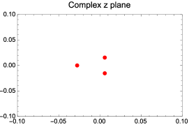
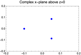
Figure 1: Two figures of the geometry deformed by $\epsilon=.001$, $a=0$, with $(p,q)$ seven-branes on the left and ramification points of the elliptic curve on the right.

where we have displayed the branes in the $z$-plane as red dots and we have also displayed the $x$-plane above $z=0$, where the blue dots represent three ramificaton points of the torus described as a double cover (as is natural in a Weierstrass model). Any straight line between two of the blue dots determines a one-cycle in the elliptic fiber above $z=0$, and by following straight line paths from $z=0$ to the seven-branes two of the ramification points will collide, determining a vanishing cycle.

Obtaining a consistent picture of the W-boson degrees of freedom throughout the moduli space requires that the geometry provides a mechanism that turns the massive W-bosons of the slightly deformed type $III$ theory to the massive W-bosons of the slightly deformed type $I_{2}$ theory. From the weak coupling limit, we know that the latter are represented by fundamental open strings. From the deformation of the type $III$ singularity performed in [5] we know that the former are three-pronged string junctions. Thus, for $\epsilon\neq 0$ small, the continual increase of $a$ from $0$ must turn string junctions into fundamental strings.

For the deformation of a type $III$ singularity the vanishing cycles were derived in [5]; they can be read off by taking straight line paths from the origin. Beginning with the left-most brane and working clockwise about $z=0$, the ordered set of vanishing cycles are $Z_{III}=\{\pi_{2},\pi_{1},\pi_{3}\}$ where these cycles are defined as

(68)

and the massive W-bosons of the broken theory are three-pronged string junctions $J_{\pm}=(\pm 1,\pm 1,\pm 1)$ which, topologically, are two spheres in the elliptic surface due to having asymptotic charge zero [6]. Pictorially, they appear as

(69)

where the black dots represent seven-branes. See [5] for more details of the intersection theory of these particular junctions, as well as their reproduction of the Dynkin diagram.

The first deformation should be thought of as a small deformation of an $SU(2)$ seven-brane theory associated with a type $III$ singularity, that is, a Higgsing. We would now like to study a deformation that corresponds to a large deformation from a type $III$ $SU(2)$ theory to a type $I_{2}$ $SU(2)$ theory (which does not Higgs the theory), and then a small deformation that Higgses the $SU(2)$ theory on the seven-brane with an $I_{2}$ singular fiber. Heuristically, the third brane of the type $III$ singularity should be far away relative to the distance between the two branes of the deformed type $I_{2}$ singularity, which in type IIB language are two D7-branes with a small splitting.

We take $a=.3i$ and $\epsilon=.001$. The difference between this deformation and the deformation of the previous paragraph is that in this case one of the three seven-branes that was originally at $z=0$ is much further away due to taking $a\neq 0$, and the question is whether the $(p,q)$ labels of the three-branes changed in the process. The geometry appears in Figure 2

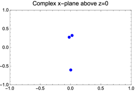
Figure 2: Two figures of the geometry deformed by $\epsilon=.001$, $a=.3i$, with $(p,q)$ seven-branes on the left and ramification points of the elliptic curve on the right.

where the brane on the left is the one that has been moved further away from the origin by turning on $a$. If one were to maintain this value of $a$ but tune $\epsilon\mapsto 0$, the two branes close to the origin would collide to give an $SU(2)$ theory with an $I_{2}$ singular fiber. Indeed, with this deformation the two-branes closer to the origin both have vanishing cycle $\pi_{1}$ and the brane displaced by the $a$ deformation has vanishing cycle $\pi_{3}$, so that now the ordered set of vanishing cycles (beginning with the left-most brane and working clockwise about $z=0$) is $Z=\{\pi_{3},\pi_{1},\pi_{1}\}$. The W-bosons of the broken $I_{2}$ $SU(2)$ theory are the strings between the $\pi_{1}$ branes, as expected since $I_{2}$ is the F-theory lift of two D7-branes.

What has happened? The natural W-boson of the broken type $III$ SU(2) theory (associated to the $a=0,\epsilon=.001$ deformation) is the three-pronged string junction, but tuning $a$ from $a=0$ to $a=.3i$ the natural W-boson of the broken type $I_{2}$ theory is the fundamental string. The change between the two different descriptions of the W-boson is a deformation induced Hanany-Witten move; for related ideas in a different geometry, see [40]. This can actually be seen via continuous deformation from $a=0$ to $a=.3i$, during which the leftmost (bottom) seven-brane in Figure 1 becomes the bottom (leftmost) seven-brane of Figure 2. In the process the straight line path from $z=0$ to the (moving) leftmost seven-brane in Figure 1 is crossed via the movement of the bottom seven-brane in Figure 1, changing the $(p,q)$ labels of the former. This matches the changes in the ordered sets of vanishing cycles.

Though we have explicitly seen the natural state change using a deformation, let us check the possibilities using the usual algebraic description of Zwiebach and Dewolfe [41] where the $(p,q)$ seven-branes are arranged in a line with branch cuts pointing downward. Technically, the branch cuts represent the mentioned straight line paths from the origin, the latter being the point whose associated fiber $E_{0}$ appears in the relative homology $H_{2}(X_{d},E_{0})$ that defines the string junctions. $X_{d}$ is the elliptic surface of the disc. The W-boson of the broken $SU(2)$ theory associated to a type $III$ singularity is

where for concreteness we choose a basis such that $\pi_{1}=(1,0)$, $\pi_{2}=(0,1)$ and $\pi_{3}=(-1,-1)$ with the convention that we cross branch cuts by moving to the right. Then the monodromy matrix associated to a $(p,q)$ seven-brane is

$$\begin{pmatrix}1-pq&&p^{2}\\ -q^{2}&&1+pq\end{pmatrix}$$ (70)

and one can check that the monodromy of these three branes reproduces the monodromy of the type $III$ singularity, as they must after deformation. We see

$$M_{\pi_{2}}M_{\pi_{3}}M_{\pi_{1}}=M_{III}=\begin{pmatrix}0&&1\\ -1&&0\end{pmatrix},$$ (71)

which is the expected behavior.

In this description, the continuous motion of the seven-branes described above amounts to the $\pi_{3}$ brane crossing the branch cut of the $\pi_{2}$ brane, changing its vanishing cycle to $M_{\pi_{3}}^{-1}\begin{pmatrix}0\\ 1\end{pmatrix}=\begin{pmatrix}-1\\ 0\end{pmatrix}$ seven-brane; but this is just $-\pi_{1}$ and we are free to call it a $\pi_{1}$ seven-brane instead if we reverse the sign of any junction coming out of the brane. With this movement and relabeling, the above junction becomes

and now the branes are in a position to do the relevant Hanany-Witten move. Prior to crossing the branch cut from the right, the $(p,q)$ charge of the piece of string that ends on the middle brane (in this picture) is $\pi_{1}+\pi_{3}$, and after the branch cut it is $\pi_{1}$ due to the monodromy action $M_{\pi_{3}}^{-1}$. If the monodromy action is replaced by a prong by pulling the string through the brane (that is, performing a Hanany-Witten move), how many extra prongs $k$ are picked up on the right-most brane? Charge conservation requires

$$\pi_{1}+\pi_{3}+k\,\pi_{3}=\pi_{1}$$ (72)

and we see $k=-1$. That is, the Hanany-Witten move replaces the portion of the string crossing the branch cut with a prong going into the $\pi_{3}$ brane. This cancels against the prong that is already there, leaving

which, since we have chosen $\pi_{1}=(1,0)$, is just a fundamental string. If we had chosen $\pi_{1}$ to be some other $(p,q)$ value this would be a $(p,q)$ string, but there is always a choice of $SL(2,\mathbb{Z})$ frame what would turn it back into a fundamental string.

In summary, we see using algebraic techniques that the natural W-boson of the Higgsed type $III$ $SU(2)$ theory, which is a three-pronged string junction, is related to the the natural W-boson of the Higgsed type $I_{2}$ $SU(2)$ theory. The relationship is a brane rearrangement together with a Hanany-Witten move, which we have seen explicitly above via two deformations of the elliptic surface with a type $III$ singular fiber.

The natural W-bosons of the type $I_{3}$ theory are (in an appropriate $SL(2,\mathbb{Z})$ duality frame) fundamental strings and the natural W-bosons of the type $IV$ theory include string junctions (see e.g. [5] for an explicit analysis). Via deformation they must be related to one another, and given the result we have just seen it is natural to expect a brane rearrangement and a Hanany-Witten move. This expectation is correct, though we will not explicitly show it since the techniques are so similar to the previous case.

We would like to present the deformation for the interested reader, though. Take

$$f=-3a^{4}+ab\,z+c\,z^{2}+f_{3}\,z^{3}\qquad\qquad g=2a^{6}-a^{3}b\,z+\left(\frac{b^{2}}{12}-a^{2}c\right)\,z^{2}+g_{3}z^{3}$$ (73)

where $a$, $b$, and $c$ are global section $a\in\mathcal{O}(-K)$, $b\in\mathcal{O}(-3K-Z)$ and $c\in\mathcal{O}(-4K-Z)$ with $Z$ is the class of $z=0$. Here $f_{3}$ and $g_{3}$ contain constant terms in $z$ as well as higher order terms. The discriminant is

$$\Delta =\frac{1}{16}z^{3}\left(1728a^{8}f_{3}+1728a^{6}g_{3}-288a^{5}bc-8a^{3}b^{3}\right)$$

$$+\frac{1}{16}z^{4}\left(-1152a^{5}bf_{3}-144a^{4}c^{2}-864a^{3}bg_{3}+120a^{2}b^{2}c+3b^{4}\right)+O(z^{5})$$ (74)

and we see that there is a gauge theory with $I_{3}$ fiber on the seven-brane at $z=0$. In the $a=0$ limit we see that

$$f=z^{2}\left(c+f_{3}z\right)\qquad\qquad g=\frac{1}{12}z^{2}\left(b^{2}+12g_{3}z\right)$$

$$\Delta=\frac{1}{16}z^{4}\left(3b^{4}+72b^{2}g_{3}z+64c^{3}z^{2}+192c^{2}f_{3}z^{3}+192cf_{3}^{2}z^{4}+64f_{3}^{3}z^{5}+432g_{3}^{2}z^{2}\right)$$ (75)

which has a gauge theory with type $IV$ Kodaira fiber on the seven-brane at $z=0$. In these cases we have not imposed the absence of outer monodromy (i.e. we have no imposed a split fiber), so they are $SU(2)$ gauge theories. If the form is further restricted so that outer monodromy is imposed, it is an $SU(3)$ gauge theory.

Extra Branes at Seven-Brane Intersections

Two seven-branes that intersect along a codimension two locus $C\subset B$ are typically only seven-branes that intersect along $C$. However, a counterexample giving rise to $SU(3)\times SU(2)$ gauge symmetry was studied in GrassiHalversonShanesonTaylor2014 where an additional brane with an $I_{1}$ singular fiber also intersected the curve of $SU(3)\times SU(2)$ intersection. Though one might have expected a $IV$-$III$ collision, a $IV$-$III$-$I_{1}$ collision occurs automatically. The Weierstrass model is $f=z^{1}t^{2}\,F$ and $g=z^{2}t^{2}\,G$ with Δ= z^3 t^4 (4t^2 F^3 + 27 z G^2 )=: z^3t^4~Δ, from which it can be seen that the brane along $\tilde{\Delta}=0$ intersects $\{z=t=0\}=:C$. Three stacks of branes intersect $C$, and we call $\tilde{\Delta}=0$ the “extra brane” at $C$.

There is a natural guess regarding the associated physics: where there is an extra brane there should be extra string (or string junction) states. In the mentioned example it was found that such a collision gives rise not only to the expected bifundamentals of $SU(3)\times SU(2)$, but also [10] fundamental hypermultiplets of $SU(3)$ and $SU(2)$ which could come in chiral multiplets if flux is turned on. Such configurations may be non-Higgsable; for example geometries, see [10, 16, 17].

Under which circumstances is there necessarily an extra brane? We take $F_{1}$ and $F_{2}$ to be the Kodaira singular fibers of seven-branes that collide along $C$, with

$$F_{1,2}\in\{II,III,IV,I_{0}^{*},IV^{*},III^{*},II^{*}\}.$$ (76)

These are the possible fibers of non-Higgsable seven-branes. Let $J_{1}$ and $J_{2}$ be the $J$-invariants associated with $F_{1}$ and $F_{2}$. By direct calculation we find:

• If either $F_{1}$ or $F_{2}$ is $I_{0}^{*}$ there is no additional brane.

• If neither $F_{1}$ nor $F_{2}$ are $I_{0}^{*}$ then there is an additional brane if and only if $J_{1}\neq J_{2}$.

• If there is an additional brane then precisely one of the fibers is type $III^{*}$ or $III$.

• If there is an additional brane and the Weierstrass model does not have $(f,g)$ vanishing to order $\geq(4,6)$ along $C$, then the fiber types are either $(IV,III)$ or $(III,II)$.

To see this, let the seven-brane with fibers $F_{1}$ and $F_{2}$ be localized on the divisors $z=0$ and $t=0$ respectively. Then write

$$f=z^{a}t^{b}\,F\qquad g=z^{c}t^{d}\,G$$ (77)

where $a,b,c,d$ can be determined from Table 1 given the knowledge of $F_{1}$ and $F_{2}$. The discriminant takes the form

$$\Delta=z^{min(3a,2c)}\,t^{min(3b,2d)}\,\,\tilde{\Delta}$$ (78)

and there is an extra brane along $C$ whenever $\tilde{\Delta}|_{z=t=0}=0$. In the cases where there are no $(4,6)$ curves, the above conclusions can all be seen directly from Table 3, where “$NF$” denotes that the $J$ invariant of $I_{0}^{*}$ is not fixed.

$F_{1}$	$F_{2}$	$J_{1}$	$J_{2}$	Minimal on $C$	$\Delta$	Additional Brane?
$IV^{*}$	$II$	$0$	$0$	Yes	$(4\tilde{f}^{3}\,t\,z+27\tilde{g}^{2})\,t^{2}\,z^{8}$	No
$I_{0}^{*}$	$IV$	$NF$	$0$	Yes	$(4\tilde{f}^{3}\,t^{2}+27\tilde{g}^{2})\,t^{4}\,z^{6}$	No
$I_{0}^{*}$	$III$	$NF$	$1$	Yes	$(4\tilde{f}^{3}+27\tilde{g}^{2}\,t)\,t^{3}\,z^{6}$	No
$I_{0}^{*}$	$II$	$NF$	$0$	Yes	$(4\tilde{f}^{3}\,t+27\tilde{g}^{2})\,t^{2}\,z^{6}$	No
$IV$	$IV$	$0$	$0$	Yes	$(4\tilde{f}^{3}\,t^{2}\,z^{2}+27\tilde{g}^{2})\,t^{4}\,z^{4}$	No
$IV$	$III$	$0$	$1$	Yes	$(4\tilde{f}^{3}\,z^{2}+27\tilde{g}^{2}\,t)\,t^{3}\,z^{4}$	Yes
$IV$	$II$	$0$	$0$	Yes	$(4\tilde{f}^{3}\,t\,z^{2}+27\tilde{g}^{2})\,t^{2}\,z^{4}$	No
$III$	$III$	$1$	$1$	Yes	$(4\tilde{f}^{3}+27\tilde{g}^{2}\,t\,z)\,t^{3}\,z^{3}$	No
$III$	$II$	$1$	$0$	Yes	$(4\tilde{f}^{3}\,t+27\tilde{g}^{2}\,z)\,t^{2}\,z^{3}$	Yes
$II$	$II$	$0$	$0$	Yes	$(4\tilde{f}^{3}\,t\,z+27\tilde{g}^{2})\,t^{2}\,z^{2}$	No

Table 3: The possible intersecting elliptic seven-branes that may arise, according to their singular fibers $F_{1}$ and $F_{2}$, and some of their properties.

3.2 Associated Matter Representations

There are two possible fiber intersections that force the existence of an extra brane, $IV$-$III$ and $III$-$II$. Due to the effects of outer monodromy, the $IV$-$III$ collision allows for the possibility of intersecting non-abelian seven-branes with $SU(3)\times SU(2)$ or $SU(2)\times SU(2)$ gauge symmetry, while intersecting seven-branes with a fiber collision $IV$-$III$ necessarily have $SU(2)$ gauge symmetry. The Lie algebra representations of matter at the $IV$-$III$-$I_{1}$ $SU(3)\times SU(2)$ collision was determined in GrassiHalversonShanesonTaylor2014. They are hypermultiplets of

$$(3,2),(3,1),(1,2)$$ (79)

in the absence of flux, but can become the chiral non-abelian $SU(3)\times SU(2)$ representations of the standard model if chirality inducing G-flux is turned on.

Let us determine the Lie algebra representations in the case of the other collision, which is $III$-$II$-$I_{1}$ via anomaly cancellation in six dimensions. Consider a six-dimensional F-theory compactification with $B_{2}=\mathbb{P}^{2}$ and a seven-brane with $SU(2)$ gauge symmetry from a type $III$ fiber on $Z=\{z=0\}$, a divisor in the hyperplane class. Take also a seven-brane with no gauge symmetry and a type $II$ singular fiber on $T=\{t=0\}$, also in the hyperplane class. Such a Weierstrass model takes the form f_12 = z   t  f_10     g_18 = z^2   t  g_15     Δ= z^3 t^2  (4f_10^3  t+27g_15^2  z)≡z^3   ~Δ and we would like to study matter at the intersection $z=\tilde{\Delta}=0$. These intersections are of two types: the single point $z=t=0$ and the $10$ points $z=f_{10}=0$ with $t\neq 0$. The latter are all points where seven-branes with a type $III$ and $I_{1}$ fiber collide; there are $2$ fundamentals of $SU(2)$ for each such point [42, 43]. Thus, the $10$ points contribute $20$ fundamental hypermultiplets. Since anomaly cancellation for an $SU(2)$ seven-brane on the hyperplane in $\mathbb{P}^{2}$ requires $22$ hypermultiplets (see e.g. section 2.5 of [44]), anomaly cancellation requires that the $III$-$II$-$I_{1}$ intersection also contribute two fundamental hypermultiplets.

Argyres-Douglas Theories on D3-branes and BPS Dyons as Junctions

D3-branes in the vicinity of seven-branes realize non-trivial $\mathcal{N}=2$ quantum field theories on their worldvolume [45], which are broken to $\mathcal{N}=1$ theories by the background. The position of the D3-brane relative to a seven-brane determines a point on the Coulomb branch of the D3-brane theory, and the seven-brane determines a singular point on the Coulomb branch at which additional particle states become massless. This point is reached when the D3-brane collides with the seven-brane, and the additional light states are string junctions that stretch from the seven-brane to the D3-brane. Previous works [46, 47] determined the string junction representations of BPS particles for well-known $\mathcal{N}=2$ theories, including $N_{f}=0,1,2,3,4$ Seiberg-Witten theory [48, 49].

In this section we will do the same for D3-branes probing the type $II$, $III$, and $IV$ singularities. Recall that the latter two are associated with the non-perturbative $SU(2)$ and $SU(3)$ theories on seven-branes that were discussed in section 3. Relative to weakly coupled realizations of $SU(2)$ and $SU(3)$ from $2$ $D7$-branes and 3 $D7$-branes, which have an $I_{2}$ and $I_{3}$ fiber in F-theory, the type $III$ and $IV$ theories have an extra seven-brane. Via studying local axiodilaton profiles we have seen that in the vicinity of the brane the string coupling is $O(1)$ and that these seven-branes source a nilpotent $SL(2,\mathbb{Z})$ monodromy. Therefore, the worldvolume theories of nearby D3-branes necessarily differ from the $N_{f}=2,3$ Seiberg-Witten theories realized on D3-branes near $I_{2}$ and $I_{3}$ seven-branes.

The worldvolume theory on a D3-brane when it has collided with a type $III$ or type $IV$ seven-brane is the $N_{f}=2$ or $3$ Seiberg-Witten theory at its Argyres-Douglas point, respectively. We will see that the characteristic [50] Argyres-Douglas (AD) phenomenon is realized by string junctions. This phenomenon is existence of points in the moduli space where electrons and dyons charged under the $U(1)$ of the $\mathcal{N}=2$ theory simultaneously become massless. In F-theory this occurs when the D3-brane collides with a type $III$ or type $IV$ seven-brane. The AD phenomenon was originally realized in $G=SU(3)$ theories, which have genus two Seiberg-Witten curves, and thus one might expect it to not exist in an elliptically fibered setup such as F-theory. For specially tuned $G=SU(2)$ Seiberg-Witten theories Argyres-Douglas points do exist [51], though; the tuning brings in an extra singularity that turns a type $I_{2}$ ($I_{3}$) fiber into a type $III$ ($IV$) fiber. Somewhat ironically, F-theory models with non-Higgsable seven-branes of type $III$ and $IV$ do not require any such tuning; the topology of the base $B$ forces the local structure of the Seiberg-Witten curve that would appear tuned from an $\mathcal{N}=2$ point of view.

We will use the BPS junction criterion of [47] to determine the BPS states on three-branes near the type $II$, $III$, and $IV$ seven-branes. This constraint is

$$(J,J)\geq-2+gcd(a(J))$$ (80)

where $J$ is the string junction and $a(J)$ is its asymptotic charge, and it is derived from the requirement that in the M-theory picture $J$ is a holomorphic curve with boundary, with the boundary a non-trivial one-cycle $a(J)$ in the smooth elliptic curve above the D3-brane. This one-cycle $a(J)$ is the asymptotic charge, and it determines the electric and magnetic charge of the associated junction under the $U(1)$ of the D3-brane theory. Junctions are relative homology cycles [6], i.e. two-cycles that may have boundary in a smooth elliptic curve above a particular point $p$. This point is given physical meaning if $p$ is the location of a D3-brane.

Throughout this section we will need a basis choice in order to represent the one-cycle $a(J)$ as a vector in $\mathbb{Z}^{2}$. We choose

$$\pi_{1}=\begin{pmatrix}1\\ 0\end{pmatrix},\qquad\pi_{3}=\begin{pmatrix}0\\ 1\end{pmatrix},$$ (81)

which determines $\pi_{2}$ via $\pi_{1}+\pi_{2}+\pi_{3}=0\in H_{1}(E_{p},\mathbb{Z})$, where $E_{p}$ is the elliptic fiber above the D3-brane in the F-theory picture, or alternatively the torus that defines the electric and magnetic charges.

3.3 The $N_{f}=1$ Argyres-Douglas Point and the Type $II$ Kodaira Fiber

Let us study the F-theory realization of BPS states on a D3-brane near a slightly deformed type $II$ Kodaira fiber. From [5], the vanishing cycles are $Z=\{\pi_{3},\pi_{1}\}$ and so the $I$-matrix that determines topological intersections is

$$I=(\cdot,\cdot)=\begin{pmatrix}-1&-\frac{1}{2}\\ -\frac{1}{2}&-1\end{pmatrix}.$$ (82)

Defining $J=(Q_{1},Q_{2})$ we have

$$(J,J)=-Q_{1}Q_{2}-Q_{1}^{2}-Q_{2}^{2}\qquad\text{with}\qquad a(J)=\begin{pmatrix}Q_{2}\\ Q_{1}\end{pmatrix}.$$ (83)

The string junctions satisfying the BPS particle condition (80) are

$a(J)$	Junctions
$(1,0)$	$(0,1)$
$(1,-1)$	$(-1,1)$
$(0,1)$	$(1,0)$

These BPS particles arising from string junctions also have BPS anti-particles via the action $J\mapsto-J$, which preserves $(J,J)$ and $gcd(a(J))$ and therefore the associated junctions $-J$ satisfy (80). In the M-theory description the geometric object $J$ corresponds to a two-cycle, and the associated BPS particle arises from wrapping an M2-brane on that cycle; the anti-particle associated to $-J$ arises from wrapping an anti M2-brane. Note that there is no junction $J$ with $a(J)=0$ and $(J,J)=-2$; as explained in [5], this demonstrates via deformation that the type II singularity does not carry a gauge algebra.

One might be tempted to think that the seven-brane associated to a type II singularity has little impact on the low energy physics of an F-theory compactification, since it does not carry any gauge algebra. However, this is not true, and we would like to emphasize:

• Locally near the type II seven-brane (or precisely in the 8d theory) the worldvolume theory on the D3-brane is $N_{f}=1$ Seiberg-Witten theory near its Argyres-Douglas point. At that point BPS electrons, monopoles, and dyons become massless.

• Since $J=0$ for the type $II$ Kodaira fiber, $g_{s}$ is $O(1)$ in the vicinity of the seven-brane, with $\tau$ profile solved via Ramanujan’s alternative bases in section 2..

• Even though both can split into two mutually non-local seven-branes, the seven-brane associated to a type II Kodaira fiber is not an orientifold. First, because their $SL(2,\mathbb{Z})$ monodromies are different, and second because the orientifold famously must split due to instanton effects in F-theory, which is not true of the type II seven-brane.

3.4 The $N_{f}=2$ Argyres-Douglas Point and the Type $III$ Kodaira Fiber

In this section we study the F-theory realization of BPS states on D3-branes near a slightly deformed type $III$ Kodaira fiber. In the coincident limit this theory is the Argyres-Douglas theory obtained by tuning $N_{f}=2$ $G=SU(2)$ Seiberg-Witten theory to its Argyres-Douglas point. Utilizing an explicit deformation of [5], the vanishing cycles are $Z=\{\pi_{2},\pi_{1},\pi_{3}\}$ and the $I$-matrix that determines topological intersections is

$$I=(\cdot,\cdot)=\begin{pmatrix}-1&\frac{1}{2}&-\frac{1}{2}\\ \frac{1}{2}&-1&\frac{1}{2}\\ -\frac{1}{2}&\frac{1}{2}&-1\end{pmatrix}.$$ (84)

Defining a string junction by $J=(Q_{1},Q_{2},Q_{3})$ we have

$$(J,J)=Q_{1}Q_{2}+Q_{1}Q_{3}-Q_{2}Q_{3}-\sum_{i}Q_{i}^{2}\qquad\text{with}\qquad a(J)=\begin{pmatrix}-Q_{1}+Q_{2}\\ -Q_{1}+Q_{3}\end{pmatrix}.$$ (85)

Thees BPS particles arising from string junctions also have BPS anti-particles via the action $J\mapsto-J$, which preserves $(J,J)$ and $gcd(a(J))$, leaving (80) invariant.

Using the constraint (80) the possible BPS string junctions can be computed directly. The states of self-intersection $-2$ have $a(J)=0$ and were identified in [5]. They are $J_{+}=(1,1,1)$ and $J_{-}=(-1,-1,-1)$, where the $\pm$ denote a choice of positive and negative root for the associated $SU(2)$ algebra that is the gauge algebra on the seven-brane and the flavor algebra of the three-brane theory. The rest of the junctions satisfying (80) have $(J,J)=-1$ and are given by

$a(J)$	Junctions
$(0,1)$	$(0,0,1)$,$(-1,-1,0)$
$(1,0)$	$(0,1,0)$,$(-1,0,-1)$
$(1,1)$	$(-1,0,0)$
$(1,-1)$	$(0,1,-1)$

where the sets of junctions in the first two lines are doublets of $SU(2)$ since they differ by $J_{\pm}$. This spectrum matches the known BPS states in the maximal chamber of the deformed theory with masses turned on; see e.g. [52].

We have seen the relationship between the ordered sets of vanishing cycles $Z=\{\pi_{2},\pi_{1},\pi_{3}\}$ of [5] and $Z=\{A,A,C\}$ of [41, 47] that can be associated to the deformed type III Kodaira fiber by explicit deformation in section 3. Let us study the BPS states with the latter set for the sake of completeness, taking

$$A=\begin{pmatrix}1\\ 0\end{pmatrix},\qquad C=\begin{pmatrix}1\\ 1\end{pmatrix},$$ (86)

as in [3]. The $I$-matrix is

$$I=(\cdot,\cdot)=\begin{pmatrix}-1&0&\frac{1}{2}\\ 0&-1&\frac{1}{2}\\ \frac{1}{2}&\frac{1}{2}&-1\end{pmatrix}$$ (87)

and taking $J=(Q_{1},Q_{2},Q_{3})$ we compute

$$(J,J)=Q_{3}(Q_{1}+Q_{2})-\sum_{i}Q_{i}^{2}\qquad\text{with}\qquad a(J)=\begin{pmatrix}Q_{1}+Q_{2}+Q_{3}\\ Q_{3}\end{pmatrix}.$$ (88)

There are junctions $J_{\pm}$ satisfying the BPS constraint (80) with $a(J)=0$ and $(J,J)=-2$. They are $J_{+}=(1,-1,0)$ and $J_{-}=(-1,1,0)$, and they are the $W_{\pm}$ bosons of the broken $SU(2)$ theory. The rest of the junctions satisfying the BPS condition have $(J,J)=-1$ and satisfy

$a(J)$	Junctions
$(3,1)$	$(1,1,1)$
$(2,1)$	$(1,0,1)$,$(0,1,1)$
$(1,1)$	$(1,0,1)$
$(1,0)$	$(1,0,0)$,$(0,1,0)$.

We again see two $SU(2)$ doublets and two $SU(2)$ singlets before taking into account the $-J$ junctions. These junctions with electromagnetic charge must be related to those of $Z=\{\pi_{2},\pi_{1},\pi_{3}\}$ by a Hanany-Witten move, as we explicitly showed for the simple roots $J_{\pm}$ in section 3.

3.5 The $N_{f}=3$ Argyres-Douglas Point and the Type $IV$ Kodaira Fiber

In this section we study the F-theory realization of BPS states on D3-branes near a slightly deformed type IV Kodaira fiber. In the coincident limit the worldvolume theory on the D3-brane is the Argyres-Douglas theory obtained by tuning $N_{f}=3$ $G=SU(2)$ Seiberg-Witten theory to its Argyres-Douglas point.

The ordered set of vanishing cycles derived in [5] is $Z_{IV}=\{\pi_{1},\pi_{3},\pi_{1},\pi_{3}\}$ and the associated I-matrix that determines the topological intersections of junctions is

$$I=(\cdot,\cdot)=\begin{pmatrix}-1&\frac{1}{2}&0&\frac{1}{2}\\ \frac{1}{2}&-1&-\frac{1}{2}&0\\ 0&-\frac{1}{2}&-1&\frac{1}{2}\\ \frac{1}{2}&0&\frac{1}{2}&-1\end{pmatrix}.$$ (89)

Writing the junction as a vector $J=(Q_{1},Q_{2},Q_{3},Q_{4})$ we have

$$(J,J)=Q_{1}Q_{2}+Q_{1}Q_{4}-Q_{2}Q_{3}+Q_{3}Q_{4}-\sum_{i}Q_{i}^{2}\qquad\text{with}\qquad a(J)=\begin{pmatrix}Q_{1}+Q_{3}\\ Q_{2}+Q_{4}\end{pmatrix}.$$ (90)

These BPS particles arising from string junctions also have BPS anti-particles via the action $J\mapsto-J$, which preserves $(J,J)$ and $a(J)$ and therefore the associated junctions $-J$ satisfy (80). The latter arise from wrapped anti M2-branes in the M-theory picture.

Let us derive the possible BPS string junctions using the constraint (80). The junctions of self-intersection $-2$ have $a(J)=0$ and were identified in [5]. They are the roots of an $SU(3)$ algebra, and we take $J_{1}=(1,0,-1,0)$ and $J_{2}=(0,1,0,-1)$ as the simple roots; then the full set of root junctions is simply $J_{1}$,$J_{2}$, $J_{1}+J_{2}$ and their negatives. Solving the condition for BPS junctions (80) we find that the possible BPS junctions are

$a(J)$	Junctions
$(-1,-1)$	$(0,0,-1,-1)$ $(-1,0,0,-1)$ $(-1,-1,0,0)$
$(1,0)$	$(1,0,0,0)$ $(0,0,1,0)$ $(0,-1,1,1)$
$(0,1)$	$(1,1,-1,0)$ $(0,1,0,0)$ $(0,0,0,1)$
$(2,1)$	$(1,0,1,1)$
$(-1,-2)$	$(-1,-1,0,-1)$
$(-1,1)$	$(0,1,-1,0)$

and we have chosen the ordering of the junctions in the first three columns to show that they are fundamentals of $SU(3)$. Namely, in each of the first thee columns the second junction subtracted from the first is $J_{1}$ and the third junction from the second is $J_{2}$. The negatives of these are anti-fundamental, completing the non-trivial flavor hypermultiplets.

I would like to thank Philip Argyres, Shaun Cooper, Andreas Malmendier, Brent Nelson, Daniel Schultz, Washington Taylor, Yi-Nan Wang and Wenbin Yan for helpful discussions and correspondence. I am particularly grateful to Antonella Grassi and Julius Shaneson for discussions and comments on a draft, and to J.L. Halverson for support and encouragement. This work is generously supported by startup funding from Northeastern University and the National Science Foundation under Grant No. PHY11-25915.

$F_{1}$	$F_{2}$	$J_{1}$	$J_{2}$	Minimal on $C$	$\Delta$	Additional Brane?
$II^{*}$	$II^{*}$	$0$	$0$	No	$(4\tilde{f}^{3}\,t^{2}\,z^{2}+27\tilde{g}^{2})\,t^{10}\,z^{10}$	No
$II^{*}$	$III^{*}$	$0$	$1$	No	$(4\tilde{f}^{3}\,z^{2}+27\tilde{g}^{2}\,t)\,t^{9}\,z^{10}$	Yes
$II^{*}$	$IV^{*}$	$0$	$0$	No	$(4\tilde{f}^{3}\,t\,z^{2}+27\tilde{g}^{2})\,t^{8}\,z^{10}$	No
$II^{*}$	$I_{0}^{*}$	$0$	$NF$	No	$(4\tilde{f}^{3}\,z^{2}+27\tilde{g}^{2})\,t^{6}\,z^{10}$	No
$II^{*}$	$IV$	$0$	$0$	No	$(4\tilde{f}^{3}\,t^{2}\,z^{2}+27\tilde{g}^{2})\,t^{4}\,z^{10}$	No
$II^{*}$	$III$	$0$	$1$	No	$(4\tilde{f}^{3}\,z^{2}+27\tilde{g}^{2}\,t)\,t^{3}\,z^{10}$	Yes
$II^{*}$	$II$	$0$	$0$	No	$(4\tilde{f}^{3}\,t\,z^{2}+27\tilde{g}^{2})\,t^{2}\,z^{10}$	No
$III^{*}$	$III^{*}$	$1$	$1$	No	$(4\tilde{f}^{3}+27\tilde{g}^{2}\,t)\,t^{9}\,z^{9}$	No
$III^{*}$	$IV^{*}$	$1$	$0$	No	$(4\tilde{f}^{3}\,t+27\tilde{g}^{2}\,z)\,t^{8}\,z^{9}$	Yes
$III^{*}$	$I_{0}^{*}$	$1$	$NF$	No	$(4\tilde{f}^{3}+27\tilde{g}^{2}\,z)\,t^{6}\,z^{9}$	No
$III^{*}$	$IV$	$1$	$0$	No	$(4\tilde{f}^{3}\,t^{2}+27\tilde{g}^{2}\,z)\,t^{4}\,z^{9}$	Yes
$III^{*}$	$III$	$1$	$1$	No	$(4\tilde{f}^{3}+27\tilde{g}^{2}\,t\,z)\,t^{3}\,z^{9}$	No
$III^{*}$	$II$	$1$	$0$	No	$(4\tilde{f}^{3}\,t+27\tilde{g}^{2}\,z)\,t^{2}\,z^{9}$	Yes
$IV^{*}$	$IV^{*}$	$0$	$0$	No	$(4\tilde{f}^{3}\,t\,z+27\tilde{g}^{2})\,t^{8}\,z^{8}$	No
$IV^{*}$	$I_{0}^{*}$	$0$	$NF$	No	$(4\tilde{f}^{3}\,z+27\tilde{g}^{2})\,t^{8}z^{8}$	No
$IV^{*}$	$IV$	$0$	$0$	No	$(4\tilde{f}^{3}\,t^{2}\,z+27\tilde{g}^{2})\,t^{4}\,z^{8}$	No
$IV^{*}$	$III$	$0$	$1$	No	$(4\tilde{f}^{3}\,z+27\tilde{g}^{2}\,t)\,t^{3}\,z^{8}$	Yes
$IV^{*}$	$II$	$0$	$0$	Yes	$(4\tilde{f}^{3}\,t\,z+27\tilde{g}^{2})\,t^{2}\,z^{8}$	No
$I_{0}^{*}$	$I_{0}^{*}$	$NF$	$NF$	No	$(4\tilde{f}^{3}+27\tilde{g}^{2})\,t^{6}\,z^{6}$	No
$I_{0}^{*}$	$IV$	$NF$	$0$	Yes	$(4\tilde{f}^{3}\,t^{2}+27\tilde{g}^{2})\,t^{4}\,z^{6}$	No
$I_{0}^{*}$	$III$	$NF$	$1$	Yes	$(4\tilde{f}^{3}+27\tilde{g}^{2}\,t)\,t^{3}\,z^{6}$	No
$I_{0}^{*}$	$II$	$NF$	$0$	Yes	$(4\tilde{f}^{3}\,t+27\tilde{g}^{2})\,t^{2}\,z^{6}$	No
$IV$	$IV$	$0$	$0$	Yes	$(4\tilde{f}^{3}\,t^{2}\,z^{2}+27\tilde{g}^{2})\,t^{4}\,z^{4}$	No
$IV$	$III$	$0$	$1$	Yes	$(4\tilde{f}^{3}\,z^{2}+27\tilde{g}^{2}\,t)\,t^{3}\,z^{4}$	Yes
$IV$	$II$	$0$	$0$	Yes	$(4\tilde{f}^{3}\,t\,z^{2}+27\tilde{g}^{2})\,t^{2}\,z^{4}$	No
$III$	$III$	$1$	$1$	Yes	$(4\tilde{f}^{3}+27\tilde{g}^{2}\,t\,z)\,t^{3}\,z^{3}$	No
$III$	$II$	$1$	$0$	Yes	$(4\tilde{f}^{3}\,t+27\tilde{g}^{2}\,z)\,t^{2}\,z^{3}$	Yes
$II$	$II$	$0$	$0$	Yes	$(4\tilde{f}^{3}\,t\,z+27\tilde{g}^{2})\,t^{2}\,z^{2}$	No

Table 4: Properties of all intersections of Kodaira fibers with finite order monodromy, including those that give rise to $(4,6)$ curves. There is an additional brane if and only if $J_{1}+J_{2}=1$, and therefore it may play an important role in local axiodilaton profiles.

References

- [1] C. Vafa, “Evidence for -theory”, Nuclear Phys. B 469, 403 (1996), http://dx.doi.org/10.1016/0550-3213(96)00172-1.
- [2] M. R. Gaberdiel & B. Zwiebach, “Exceptional groups from open strings”, Nuclear Phys. B 518, 151 (1998), http://dx.doi.org/10.1016/S0550-3213(97)00841-9.
- [3] O. DeWolfe & B. Zwiebach, “String junctions for arbitrary Lie algebra representations”, Nucl. Phys. B541, 509 (1999), hep-th/9804210.
- [4] A. Grassi, J. Halverson & J. L. Shaneson, “Matter From Geometry Without Resolution”, JHEP 1310, 205 (2013), arXiv:1306.1832.
- [5] A. Grassi, J. Halverson & J. L. Shaneson, “Non-Abelian Gauge Symmetry and the Higgs Mechanism in F-theory”, Commun. Math. Phys. 336, 1231 (2015), arXiv:1402.5962.
- [6] A. Grassi, J. Halverson & J. L. Shaneson, “Geometry and Topology of String Junctions”, arXiv:1410.6817.
- [7] A. P. Braun & T. Watari, “The Vertical, the Horizontal and the Rest: anatomy of the middle cohomology of Calabi-Yau fourfolds and F-theory applications”, JHEP 1501, 047 (2015), arXiv:1408.6167.
- [8] T. Watari, “Statistics of Flux Vacua for Particle Physics”, arXiv:1506.08433.
- [9] D. R. Morrison & C. Vafa, “Compactifications of -theory on Calabi-Yau threefolds. I, II”, Nuclear Phys. B 473, 476, 74 (1996).
- [10] A. Grassi, J. Halverson, J. Shaneson & W. Taylor, “Non-Higgsable QCD and the Standard Model Spectrum in F-theory”, arXiv::1409.8295.
- [11] S. Cecotti, C. Cordova, J. J. Heckman & C. Vafa, “T-Branes and Monodromy”, JHEP 1107, 030 (2011), arXiv:1010.5780.
- [12] D. R. Morrison & W. Taylor, “Toric bases for 6D F-theory models”, Fortsch. Phys. 60, 1187 (2012), arXiv:1204.0283.
- [13] D. R. Morrison & W. Taylor, “Classifying bases for 6D F-theory models”, Central Eur. J. Phys. 10, 1072 (2012), arXiv:1201.1943.
- [14] L. B. Anderson & W. Taylor, “Geometric constraints in dual F-theory and heterotic string compactifications”, JHEP 1408, 025 (2014), arXiv:1405.2074.
- [15] D. R. Morrison & W. Taylor, “Non-Higgsable clusters for 4D F-theory models”, JHEP 1505, 080 (2015), arXiv:1412.6112.
- [16] J. Halverson & W. Taylor, “-bundle bases and the prevalence of non-Higgsable structure in 4D F-theory models”, JHEP 1509, 086 (2015), arXiv:1506.03204.
- [17] W. Taylor & Y.-N. Wang, “A Monte Carlo exploration of threefold base geometries for 4d F-theory vacua”, JHEP 1601, 137 (2016), arXiv:1510.04978.
- [18] N. Nakayama, “On Weierstrass models”, in “Algebraic geometry and commutative algebra, Vol. II”, Kinokuniya (1988), Tokyo, p. 405–431.
- [19] K. Kodaira, “On the structure of compact complex analytic surfaces. I”, Amer. J. Math. 86, 751 (1964).
- [20] K. Kodaira, “On the structure of compact complex analytic surfaces. II”, Amer. J. Math. 88, 682 (1966).
- [21] K. Kodaira, “On the structure of compact complex analytic surfaces. III”, Amer. J. Math. 90, 55 (1968).
- [22] D. R. Morrison & C. Vafa, “Compactifications of F theory on Calabi-Yau threefolds. 2.”, Nucl. Phys. B476, 437 (1996), hep-th/9603161.
- [23] W. Taylor & Y.-N. Wang, “The F-theory geometry with most flux vacua”, JHEP 1512, 164 (2015), arXiv:1511.03209.
- [24] S. Ashok & M. R. Douglas, “Counting flux vacua”, JHEP 0401, 060 (2004), hep-th/0307049.
- [25] F. Denef & M. R. Douglas, “Distributions of flux vacua”, JHEP 0405, 072 (2004), hep-th/0404116.
- [26] W. Taylor & Y.-N. Wang, “A Monte Carlo exploration of threefold base geometries for 4d F-theory vacua”, arXiv:1510.04978.
- [27] S. Ramanujan, “Notebooks. Vols. 1, 2”, Tata Institute of Fundamental Research, Bombay (1957), p. Vol. 1. vi+351 pp.; Vol. 2. vi+393.
- [28] B. C. Berndt, S. Bhargava & F. G. Garvan, “Ramanujan’s theories of elliptic functions to alternative bases”, Trans. Amer. Math. Soc. 347, 4163 (1995), http://dx.doi.org/10.2307/2155035.
- [29] B. C. Berndt, “Ramanujan’s notebooks. Part III”, Springer-Verlag, New York (1991), p. xiv+510.
- [30] J. M. Borwein & P. B. Borwein, “A remarkable cubic mean iteration”, in “Computational methods and function theory (Valparaíso, 1989)”, Springer, Berlin (1990), p. 27–31, http://dx.doi.org/10.1007/BFb0087894.
- [31] J. M. Borwein & P. B. Borwein, “A cubic counterpart of Jacobi’s identity and the AGM”, Trans. Amer. Math. Soc. 323, 691 (1991), http://dx.doi.org/10.2307/2001551.
- [32] J. Borwein, P. Borwein & F. Garvan, “Hypergeometric analogues of the arithmetic-geometric mean iteration”, Constr. Approx. 9, 509 (1993), http://dx.doi.org/10.1007/BF01204654.
- [33] J. M. Borwein, P. B. Borwein & F. G. Garvan, “Some cubic modular identities of Ramanujan”, Trans. Amer. Math. Soc. 343, 35 (1994), http://dx.doi.org/10.2307/2154520.
- [34] B. C. Berndt, H. H. Chan & W.-C. Liaw, “On Ramanujan’s quartic theory of elliptic functions”, J. Number Theory 88, 129 (2001), http://dx.doi.org/10.1006/jnth.2000.2615.
- [35] D. Schultz, “Cubic theta functions”, Adv. Math. 248, 618 (2013), http://dx.doi.org/10.1016/j.aim.2013.08.021.
- [36] S. Cooper, “Inversion formulas for elliptic functions”, Proc. Lond. Math. Soc. (3) 99, 461 (2009), http://dx.doi.org/10.1112/plms/pdp007.
- [37] A. Sen, “F theory and orientifolds”, Nucl. Phys. B475, 562 (1996), hep-th/9605150.
- [38] A. Sen, “Orientifold limit of F theory vacua”, Phys. Rev. D55, 7345 (1997), hep-th/9702165.
- [39] K. Dasgupta & S. Mukhi, “F theory at constant coupling”, Phys. Lett. B385, 125 (1996), hep-th/9606044.
- [40] M. Cvetic, I. Garcia-Etxebarria & J. Halverson, “Global F-theory Models: Instantons and Gauge Dynamics”, JHEP 1101, 073 (2011), arXiv:1003.5337.
- [41] O. DeWolfe & B. Zwiebach, “String junctions for arbitrary Lie-algebra representations”, Nuclear Phys. B 541, 509 (1999), http://dx.doi.org/10.1016/S0550-3213(98)00743-3.
- [42] A. Grassi & D. R. Morrison, “Group representations and the Euler characteristic of elliptically fibered Calabi-Yau threefolds”, math/0005196.
- [43] A. Grassi & D. R. Morrison, “Anomalies and the Euler characteristic of elliptic Calabi-Yau threefolds”, Commun. Num. Theor. Phys. 6, 51 (2012), arXiv:1109.0042.
- [44] S. B. Johnson & W. Taylor, “Calabi-Yau threefolds with large ”, JHEP 1410, 23 (2014), arXiv:1406.0514.
- [45] T. Banks, M. R. Douglas & N. Seiberg, “Probing F theory with branes”, Phys. Lett. B387, 278 (1996), hep-th/9605199.
- [46] A. Mikhailov, N. Nekrasov & S. Sethi, “Geometric realizations of BPS states in N=2 theories”, Nucl. Phys. B531, 345 (1998), hep-th/9803142.
- [47] O. DeWolfe, T. Hauer, A. Iqbal & B. Zwiebach, “Constraints on the BPS spectrum of N=2, D = 4 theories with A-D-E flavor symmetry”, Nucl. Phys. B534, 261 (1998), hep-th/9805220.
- [48] N. Seiberg & E. Witten, “Electric - magnetic duality, monopole condensation, and confinement in N=2 supersymmetric Yang-Mills theory”, Nucl. Phys. B426, 19 (1994), hep-th/9407087, [Erratum: Nucl. Phys.B430,485(1994)].
- [49] N. Seiberg & E. Witten, “Monopoles, duality and chiral symmetry breaking in N=2 supersymmetric QCD”, Nucl. Phys. B431, 484 (1994), hep-th/9408099.
- [50] P. C. Argyres & M. R. Douglas, “New phenomena in SU(3) supersymmetric gauge theory”, Nucl. Phys. B448, 93 (1995), hep-th/9505062.
- [51] P. C. Argyres, M. R. Plesser, N. Seiberg & E. Witten, “New N=2 superconformal field theories in four-dimensions”, Nucl. Phys. B461, 71 (1996), hep-th/9511154.
- [52] K. Maruyoshi, C. Y. Park & W. Yan, “BPS spectrum of Argyres-Douglas theory via spectral network”, JHEP 1312, 092 (2013), arXiv:1309.3050.