Depth Superresolution using Motion Adaptive Regularization

Abstract

Spatial resolution of depth sensors is often significantly lower compared to that of conventional optical cameras. Recent work has explored the idea of improving the resolution of depth using higher resolution intensity as a side information. In this paper, we demonstrate that further incorporating temporal information in videos can significantly improve the results. In particular, we propose a novel approach that improves depth resolution, exploiting the space-time redundancy in the depth and intensity using motion-adaptive low-rank regularization. Experiments confirm that the proposed approach substantially improves the quality of the estimated high-resolution depth. Our approach can be a first component in systems using vision techniques that rely on high resolution depth information.

1 Introduction

One of the important challenges in computer vision applications is obtaining high resolution depth maps of observed scenes. A number of common tasks, such as object reconstruction, robotic navigation, and automotive driver assistance can be significantly improved by complementing intensity information from optical cameras with high resolution depth maps. However, with current sensor technology, direct acquisition of high-resolution depth maps is very expensive.

The cost and limited availability of such sensors imposes significant constraints on the capabilities of vision systems and has dampened the adoption of methods that rely on high-resolution depth maps. Thus, the literature has flourished with methods that provide numerical alternatives to boost the spatial resolution of the measured depth data.

Figure 1: Our motion adaptive method recovers a high-resolution depth sequence from high-resolution intensity and low-resolution depth sequences by imposing rank constraints on the depth patches: (a) and (b) $t$-$y$ slices of the color and depth sequences, respectively, at a fixed $x$; (c)–(e) $x$-$y$ slices at $t_{1}=10$; (f)–(h) $x$-$y$ slices at $t_{2}=40$; (c) and (f) input color images; (d) and (g) input low-resolution and noisy depth images; (e) and (h) estimated depth images.

One of the most popular and widely investigated class of techniques for improving the spatial resolution of depth is guided depth superresolution. These techniques jointly acquire the scene using a low-resolution depth sensor and a high-resolution optical camera. The information acquired from the camera is subsequently used to superresolve the low-resolution depth map. These techniques exploit the property that both modalities share common features, such as edges and joint texture changes. Thus, such features in the optical camera data provide information and guidance that significantly enhances the superresolved depth map.

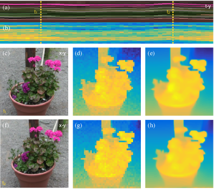
To-date, most of these methods operate on a single snapshot of the optical image and the low-resolution depth map. However, most practical uses of such systems acquire a video from the optical camera and a sequence of snapshots of the depth map. The key insight in our paper is that information about one particular frame is replicated, in some form, in nearby frames. Thus, frames across time can be exploited to superresolve the depth map and significantly improve such methods. The challenge is finding this information in the presence of scene, camera, and object motion between frames. Figure 1 provides an example, illustrating the similarity of images and depth maps across frames.

A key challenge in incorporating time into depth estimation is that depth images change significantly between frames. This results in abrupt variations in pixel values along the temporal dimension and may lead to significant degradation in the quality of the result. Thus, it is important to compensate for motion during estimation. To that end, the method we propose exploits space-time similarities in the data using motion adaptive regularization. Specifically, we identify and group similar depth patches, which we superresolve and regularize using a rank penalty.

Our method builds upon prior work on patch-based methods and low-rank regularization, which were successfully applied to a variety of practical estimation problems. It further exploits the availability of optical images which provide a very robust guide to identify and group similar patches, even if the depth map has very low resolution. Thus, the output of our iterative algorithms is robust to operating conditions. Our key contributions are summarized as follows:

• We provide a new formulation for guided depth superresolution, incorporating temporal information. In this formulation, the high resolution depth is determined by solving an inverse problem that minimizes a cost. This cost includes a quadratic data-fidelity term, as well as a new motion adaptive regularizer based on a low-rank penalty on groups of similar patches.

• We develop two optimization strategies for solving our estimation problem. The first approach is based on exact optimization of the cost via alternating direction method of multipliers (ADMM). The second approach uses a simplified algorithm that alternates between enforcing data-consistency and low-rank penalty.

• We validate our approach experimentally and demonstrate it delivers substantial improvements. In particular, we compare several algorithmic solutions to the problem and demonstrate that: (a) availability of temporal information significantly improves the quality of estimated depth; (b) motion adaptive regularization is crucial for avoiding artifacts along temporal dimension; (c) using intensity during block matching is essential for optimal performance.

2 Related Work

In the last decade, guided depth superresolution has received significant attention. Early work by Diebel and Thrun [1] showed the potential of the approach by modeling the co-occurence of edges in depth and intensity with Markov Random Fields (MRF). Kopf et al. [2] and Yang et al. [3] have independently proposed an alternative approach based on joint bilaterial filtering, where intensity is used to set the weights of the filter. The bilaterial filtering approach was further refined by Chan et al. [4] who incorporated the local statistics of the depth and by Liu et al. [5] who used geodesic distances for determining the weights. Dolson et al. [6] extended the approach to dynamic sequences to compensate for different data rates in the depth and intensity sensors. He et al. [7, 8] proposed a guided image filtering approach, improving edge preservation.

More recently, sparsity-promoting regularization—an essential component of compressive sensing [9, 10]—has provided more dramatic improvements in the quality of depth superresolution. For example, Li et al. [11] demonstrated improvements by combining dictionary learning and sparse coding algorithms. Ferstl et al. [12] relied on weighted total generalized variation (TGV) regularization for imposing a piecewise polynomial structure on depth. Gong et al. [13] combined the conventional MRF approach with an additional term promoting transform domain sparsity of the depth in an analysis form. In their recent work, Huang et al. [14] use the MRF model to jointly segment the objects and recover a higher quality depth. Schuon et al. [15] performed depth superresolution by taking several snapshots of a static scene from slightly displaced viewpoints and merging the measurements using sparsity of the weighted gradient of the depth.

Many natural images contain repetitions of similar patterns and textures. Current state-the-art image denoising methods such as nonlocal means (NLM) [16] and block matching and 3D filtering (BM3D) [17] take advantage of this redundancy by processing the image as a structured collection of patches. The original formulation of NLM was extended by Yang and Jacob [18] to more general inverse problems via introduction of specific NLM regularizers. Similarly, Danielyan et al. [19] have proposed a variational approach for general BM3D-based image reconstruction that inspired the current work. In the context of guided depth superresolution, NLM was used by Huhle et al. [20] and Park et al. [21] for reducing the amount of noise in the estimated depth. Lu et al. [22] combined a block-matching procedure with low-rank constraints for enhancing the resolution of a single depth image.

Our paper extends prior work on depth supperresolution by introducing a new variational formulation that imposes low-rank constraints in the regularization. Furthermore, our formulation is motion-adaptive, resulting in substantial improvement of the quality of the estimated depth.

3 Proposed Approach

Our approach estimates the high-resolution depth map by minimizing a cost function that—as typical in such problems—combines a data-fidelity term and a regularizer. Specifically, we impose a quadratic data fidelity term that controls the error between the measured and estimated depth values. The regularizer groups similar depth patches from multiple frames and penalizes the rank of the resulting structure. Since we use patches from multiple frames, our method is implicitly motion adaptive. Thus, by effectively combining multiple views of the scene, it yields improved depth estimates.

Figure 2: Illustration of the block matching within a space-time search area. The area in the current frame $t$ is centered at the reference patch. Search is also conducted in the same window position in multiple temporally adjacent frames. Similar patches are grouped together to construct a block $\bm{\beta}_{p}=\mathbf{B}_{p}\bm{\phi}$.

3.1 Problem Formulation

The depth sensing system collects a set of measurements denoted $\{\bm{\psi}_{t}\}_{t\in[1\dots T]}$. Each measurement is considered as a downsampled version of a higher resolution depth map $\bm{\phi}_{t}\in\mathbb{R}^{N}$ using a subsampling operator $\mathbf{H}_{t}$. Our end goal is to recover this high-resolution depth map $\bm{\phi}_{t}$ for all $t$.

In the remainder of this work, we use $N$ to denote the number of pixels in each frame, $T$ to denote the number of temporal frames, and $M$ to denote the total number of depth measurements. Furthermore, $\bm{\psi}\in\mathbb{R}^{M}$ denotes the vector of all the measurements, $\bm{\phi}\in\mathbb{R}^{NT}$ the complete sequence of high-resolution depth maps, and $\mathbf{H}\in\mathbb{R}^{M\times NT}$ the complete subsampling operator. We also have available the sequence of high-resolution intensity images from the optical camera, denoted $\mathbf{x}\in\mathbb{R}^{NT}$.

Using the above, a forward model for the depth recovery problem is given by

$$\bm{\psi}=\mathbf{H}\bm{\phi}+\mathbf{e},$$ (1)

where $\mathbf{e}\in\mathbb{R}^{M}$ denotes the measurement noise. Thus, our objective becomes to recover high-resolution depth given the measured data $\bm{\psi}$ and $\mathbf{x}$, and the sampling operator $\mathbf{H}$.

As typical in such problems, we formulate the depth estimation task as an optimization problem

$$\widehat{\bm{\phi}}=\mathop{\mathrm{arg\,min}}_{\bm{\phi}\in\mathbb{R}^{NT}}\left\{\frac{1}{2}\|\bm{\psi}-\mathbf{H}\bm{\phi}\|_{\ell_{2}}^{2}+\sum_{p=1}^{P}\mathcal{R}(\mathbf{B}_{p}\bm{\phi})\right\},$$ (2)

where $\frac{1}{2}\|\bm{\psi}-\mathbf{H}\bm{\phi}\|_{\ell_{2}}^{2}$ enforces data fidelity and $\sum_{p=1}^{P}\mathcal{R}(\mathbf{B}_{p}\bm{\phi})$ is a regularization term that imposes prior knowledge about the depth map.

We form the regularization term by constructing sets of patches from the image. Specifically, we first define an operator $\mathbf{B}_{p}$, for each set of patches $p\in[1,\dots,P]$, where $P$ is the number of such sets constructed. The operator extracts $L$ patches of size $B$ pixels from the depth image frames in $\bm{\phi}$. As illustrated in Fig. 2, each block $\bm{\beta}_{p}=\mathbf{B}_{p}\bm{\phi}\in\mathbb{R}^{B\times L}$ is obtained by first selecting a reference patch and then finding $L-1$ similar patches within the current frame as well as the adjacent temporal frames.

To determine similarity and to group similar patches together we use the intensity image as a guide. To reduce the computational complexity of the search, we restrict it to a space-time window of fixed size around the reference patch. We perform the same block matching procedure for the whole space-time image by moving the reference patch and by considering overlapping patches in each frame. Thus, each pixel in the signal $\bm{\phi}$ may contribute to multiple blocks.

The adjoint $\mathbf{B}^{T}_{p}$ of $\mathbf{B}_{p}$ simply corresponds to placing the patches in the block back to their original locations in $\bm{\phi}$. It satisfies the following property

$$\sum_{p=1}^{P}\mathbf{B}^{T}_{p}\mathbf{B}_{p}=\mathbf{R},$$ (3)

where $\mathbf{R}=\mathrm{diag}(r_{1},\dots,r_{N})\in\mathbb{R}^{NT\times NT}$ and $r_{n}$ denotes the total number of references to the $n$th pixel by the matrices $\{\mathbf{B}_{p}\}_{p=1,\dots,P}$. Therefore, the depth image $\bm{\phi}$ can be expressed in terms of an overcomplete representation using the blocks

$$\bm{\phi}=\mathbf{R}^{-1}\sum_{p=1}^{P}\mathbf{B}_{p}^{T}\mathbf{B}_{p}\bm{\phi}.$$ (4)

3.2 Rank regularization

Each block, represented as a matrix, contains multiple similar patches, i.e., similar columns. Thus, we expect the matrix to have a low rank, making rank a natural regularizer for the problem

$$\mathcal{R}(\bm{\beta})=\mathrm{rank}(\bm{\beta}).\quad(\bm{\beta}\in\mathbb{R}^{B\times L})$$ (5)

By seeking a low-rank solution to (2), we exploit the similarity of blocks to guide superresolution while enforcing consistency with the observed data. However, the rank regularizer (5) is of little practical interest since its direct optimization is intractable. The most popular approach around this, first proposed by Fazel in [23], is to convexify the rank by replacing it with the nuclear norm:

$$\mathcal{R}(\bm{\beta})=\lambda\|\bm{\beta}\|_{\ast}\,\triangleq\,\lambda\sum_{k=1}^{\min(B,L)}\sigma_{k}(\bm{\beta}),$$ (6)

where $\sigma_{k}(\bm{\beta})$ denotes the $k$th largest singular value of $\bm{\beta}$ and $\lambda>0$ is a parameter controlling the amount of regularization.

In addition to its convexity, the nuclear norm is an appealing penalty to optimize because it also has a closed form proximal operator:

$$\mathrm{prox}_{\lambda\|\cdot\|_{\ast}} (\bm{\psi})\,\triangleq\,\mathop{\mathrm{arg\,min}}_{\bm{\beta}\in\mathbb{R}^{B\times L}}\left\{\frac{1}{2}\|\bm{\psi}-\bm{\beta}\|_{F}^{2}+\lambda\|\bm{\beta}\|_{\ast}\right\}$$

$$=\mathbf{u}\,\eta_{\lambda}(\bm{\sigma}(\bm{\psi}))\,\mathbf{v}^{T},$$ (7)

where $\bm{\psi}=\mathbf{u}\bm{\sigma}\mathbf{v}^{T}$ is the singular value decomposition (SVD) of $\bm{\psi}$ and $\eta_{\lambda}$ is the soft-thresholding function applied to the diagonal matrix $\bm{\sigma}$.

Figure 3: Illustration of the $\nu$-shrinkage operator $\mathcal{T}_{\nu,\lambda}$ for a fixed $\lambda=1$ at two values of $\nu$. For $\nu=1$ the shrinkage is equivalent to soft-thresholding, while for $\nu\rightarrow 0$ it approaches hard-thresholding

Recent work has shown that nonconvex regularizers consistently outperform nuclear norm by providing stronger denoising capability without losing important signal compoenents [24, 25, 26]. In this paper, we use the nonconvex generalization to the nuclear norm proposed by Chartrand [24]

$$\mathcal{R}(\bm{\beta})=\lambda\mathcal{G}_{\lambda,\nu}(\bm{\beta})\,\triangleq\,\lambda\sum_{k=1}^{\min(B,L)}g_{\lambda,\nu}(\sigma_{k}(\bm{\beta})),$$ (8)

Here, the scalar function $g_{\lambda,\nu}$ is designed to satisfy

$$\min_{x\in\mathbb{R}}\left\{\frac{1}{2}|x-y|^{2}+\lambda g_{\lambda,\nu}(x)\right\}=h_{\lambda,\nu}(x),$$ (9)

where $h_{\lambda,\nu}$ is the $\nu$-Huber function

$$h_{\lambda,\nu}(x)\,\triangleq\,\begin{cases}\frac{|x|^{2}}{2\lambda}&\text{if }|x|<\lambda^{1/(2-\nu)}\\ \frac{|x|^{\nu}}{\nu}-\delta&\text{if }|x|\geq\lambda^{1/(2-\nu)},\end{cases}$$ (10)

with $\delta\,\triangleq\,(1/\nu-1/2)\lambda^{\nu/(2-\nu)}$. Although $g_{\lambda,\nu}$ is nonconvex and has no closed form formula, its proximal operator does admit a closed form expression

$$\mathrm{prox}_{\lambda\mathcal{G}_{\lambda,\nu}} (\bm{\psi})\,\triangleq\,\mathop{\mathrm{arg\,min}}_{\bm{\beta}\in\mathbb{R}^{B\times L}}\left\{\frac{1}{2}\|\bm{\psi}-\bm{\beta}\|_{F}^{2}+\lambda\mathcal{G}_{\lambda,\nu}(\bm{\beta})\right\}$$

$$=\mathbf{u}\,\mathcal{T}_{\lambda,\nu}(\bm{\sigma}(\bm{\psi}))\,\mathbf{v}^{T},$$ (11)

where $\mathcal{T}_{\lambda,\nu}$ is a poitwise $\nu$-shrinkage operator defined as

$$\mathcal{T}_{\lambda,\nu}(x)\,\triangleq\,\max(0,|x|-\lambda|x|^{\nu-1})\frac{x}{|x|}.$$ (12)

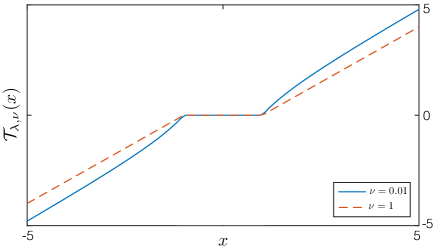
For $\nu=1$, $\nu$-shrinkage (12) is equivalent to conventional soft thresholding (See illustration in Fig. 3). When $\nu\rightarrow 0$, it approaches hard thresholding, which is similar to principal component analysis (PCA) in the sense that it retains the significant few principal components.

Thus, the regularizer (8) is a computationally tractable alternative to the rank penalty. While the regularizer is not convex, it can still be efficiently optimized due to closed form of its proximal operator (3.2). Note that due to nonconvexity of our regularizer for $\eta<1$, it is difficult to theoretically guarantee global convergence. However, we have empirically observed that our algorithms converge reliably over a broad spectrum of examples presented in Section 4.

3.3 Iterative optimization

To solve the optimization problem (2) under the rank regularizer (8), we first simplify notation by defining an operator $\mathbf{B}\,\triangleq\,(\mathbf{B}_{1},\dots,\mathbf{B}_{P})$ and a vector ${\bm{\beta}\,\triangleq\,\mathbf{B}\bm{\phi}=(\bm{\beta}_{1},\dots,\bm{\beta}_{P})}$.

The minimization is performed using an augmented-Lagrangian (AL) method [27]. Specifically, we seek the critical points of the following AL

$$\mathcal{L}(\bm{\phi},\bm{\beta},\bm{s}) \,\triangleq\,\frac{1}{2}\|\bm{\psi}-\mathbf{H}\bm{\phi}\|_{\ell_{2}}^{2}+\sum_{p=1}^{P}\mathcal{R}(\bm{\beta}_{p})$$ (13a)

$$+\frac{\rho}{2}\|\bm{\beta}-\mathbf{B}\bm{\phi}\|_{\ell_{2}}^{2}+\bm{s}^{T}(\bm{\beta}-\mathbf{B}\bm{\phi})$$

$$=\frac{1}{2}\|\bm{\psi}-\mathbf{H}\bm{\phi}\|_{\ell_{2}}^{2}+\sum_{p=1}^{P}\mathcal{R}(\bm{\beta}_{p})$$ (13b)

$$+\frac{\rho}{2}\|\bm{\beta}-\mathbf{B}\bm{\phi}+\bm{s}/\rho\|_{\ell_{2}}^{2}-\frac{1}{2\rho}\|\bm{s}\|_{\ell_{2}}^{2},$$

where $\rho>0$ is the quadratic parameter and $\bm{s}$ is the dual variable that imposes the constraint $\bm{\beta}=\mathbf{B}\bm{\phi}$. Traditionally, an AL scheme solves (2) by alternating between a joint minimization step and an update step as

$$(\bm{\phi}^{k},\bm{\beta}^{k}) \leftarrow\mathop{\mathrm{arg\,min}}_{\bm{\phi}\in\mathbb{R}^{NT},\bm{\beta}\in\mathbb{R}^{P\times B\times L}}\left\{\mathcal{L}(\bm{\phi},\bm{\beta},\bm{s}^{k-1})\right\}$$ (14a)

$$\bm{s}^{k} \leftarrow\bm{s}^{k-1}+\rho(\bm{\beta}^{k}-\mathbf{B}\bm{\phi}^{k}).$$ (14b)

However, the joint minimization step (14a) is typically computationally intensive. To reduce complexity, we separate (14a) into a succession of simpler steps using the well-established by now alternating direction method of multipliers (ADMM) [28]. The steps are as follows

$$\bm{\phi}^{k} \leftarrow\mathop{\mathrm{arg\,min}}_{\bm{\phi}\in\mathbb{R}^{NT}}\left\{\mathcal{L}(\bm{\phi},\bm{\beta}^{k-1},\bm{s}^{k-1})\right\}$$ (15a)

$$\bm{\beta}^{k} \leftarrow\mathop{\mathrm{arg\,min}}_{\bm{\beta}\in\mathbb{R}^{P\times B\times L}}\left\{\mathcal{L}(\bm{\phi}^{k},\bm{\beta},\bm{s}^{k-1})\right\}$$ (15b)

$$\bm{s}^{k} \leftarrow\bm{s}^{k-1}+\rho(\bm{\beta}^{k}-\mathbf{B}\bm{\phi}^{k}).$$ (15c)

By ignoring the terms that do not depend on $\bm{\phi}$, (15a) amounts to solving a quadratic problem

$$\bm{\phi}^{k} \leftarrow\mathop{\mathrm{arg\,min}}_{\bm{\phi}\in\mathbb{R}^{NT}}\left\{\frac{1}{2}\|\bm{\psi}-\mathbf{H}\bm{\phi}\|_{\ell_{2}}^{2}+\frac{\rho}{2}\|\mathbf{B}\bm{\phi}-\mathbf{z}^{k-1}\|_{\ell_{2}}^{2}\right\}$$

$$\leftarrow(\mathbf{H}^{T}\mathbf{H}+\rho\mathbf{B}^{T}\mathbf{B})^{-1}(\mathbf{H}\bm{\psi}+\rho\mathbf{B}^{T}\mathbf{z}^{k-1}),$$ (16)

where $\mathbf{z}^{k-1}\,\triangleq\,\bm{\beta}^{k-1}+\bm{s}^{k-1}/\rho$. Solving this quadratic equation is efficient since the inversion is performed on a diagonal matrix. Similarly, (15b) is solved by

$$\bm{\beta}^{k}\leftarrow\mathop{\mathrm{arg\,min}}_{\bm{\beta}\in\mathbb{R}^{P\times B\times L}}\left\{\frac{\rho}{2}\|\bm{\beta}-\mathbf{y}^{k}\|_{\ell_{2}}^{2}+\sum_{p=1}^{P}\mathcal{R}(\bm{\beta}_{p})\right\},$$ (17)

with $\mathbf{y}^{k}\,\triangleq\,\mathbf{B}\bm{\phi}^{k}-\bm{s}^{k-1}/\rho$. This step can be solved via block-wise application of the proximal operator (3.2) as

$$\bm{\beta}_{p}^{k}\leftarrow\mathrm{prox}_{(\lambda/\rho)\mathcal{G}_{\lambda,\nu}}(\mathbf{B}_{p}\bm{\phi}^{k}-\bm{s}_{p}^{k-1}/\rho),$$ (18)

for all $p\in[1,\dots,P]$.

3.4 Simplified algorithm

The algorithm in Section 3.3 can be significantly simplified by decoupling the enforcement of the data-fidelity from the enforcement of the rank-based regularization. The simplified algorithm reduces computational complexity while making estimation more uniform across the whole space-time depth image.

In particular, Danielyan [29] has argued that, due to inhomogeneous distribution of pixel references generated by matching across the image, using a penalty with a single regularization parameter highly penalizes pixels with a large number of references. The resulting nonuniform regularization makes the algorithm potentially oversensitive to the choice of the parameter $\lambda$. Instead, we rely on the simplified algorithm

$$\bm{\beta}_{p}^{k} \leftarrow\mathop{\mathrm{arg\,min}}_{\bm{\beta}_{p}\in\mathbb{R}^{B\times L}}\left\{\frac{1}{2}\|\bm{\beta}_{p}-\mathbf{B}_{p}\bm{\phi}^{k-1}\|_{F}^{2}+\mathcal{R}(\bm{\beta}_{p})\right\}$$ (19a)

$$\bm{\phi}^{k} \leftarrow\mathop{\mathrm{arg\,min}}_{\bm{\phi}\in\mathbb{R}^{NT}}\left\{\frac{1}{2}\|\bm{\psi}-\mathbf{H}\bm{\phi}\|_{\ell_{2}}^{2}+\frac{\rho}{2}\|\bm{\phi}-\tilde{\bm{\phi}}^{k}\|_{\ell_{2}}^{2}\right\}$$ (19b)

where $\tilde{\bm{\phi}}^{k}\,\triangleq\,\mathbf{R}^{-1}\mathbf{B}^{T}\bm{\beta}^{k}$, and $\lambda>0$ is the regularization and $\rho>0$ is the quadratic parameters.

To solve (19a) we apply the proximal operator

$$\bm{\beta}_{p}^{k}\leftarrow\mathrm{prox}_{\lambda\mathcal{G}_{\lambda,\nu}}(\mathbf{B}_{p}\bm{\phi}^{k-1}),$$ (20)

for all $p\in[1,\dots,P]$. Next, (19b) reduces to a linear step

$$\bm{\phi}^{k}\leftarrow(\mathbf{H}^{T}\mathbf{H}+\rho\mathbf{I})^{-1}(\mathbf{H}^{T}\bm{\psi}+\rho\tilde{\bm{\phi}}^{k}).$$ (21)

There are substantial similarities between algorithms (15) and (19). The main differences are that we eliminated the dual variable $\bm{s}$ and simplified the quadratic subproblem (16).

4 Experimens

	Flower				Lawn				Road
	$2\times$	$3\times$	$4\times$	$5\times$	$2\times$	$3\times$	$4\times$	$5\times$	$2\times$	$3\times$	$4\times$	$5\times$
Linear	$25.62$	$22.81$	$21.07$	$20.15$	$28.32$	$25.89$	$24.32$	$23.05$	$25.44$	$22.78$	$21.16$	$20.18$
TV-2D	$26.52$	$23.17$	$21.30$	$20.32$	$29.97$	$26.56$	$24.70$	$23.31$	$26.30$	$23.21$	$21.44$	$20.38$
WTGV-2D	$26.73$	$23.54$	$21.68$	$20.66$	$30.16$	$26.87$	$24.94$	$23.66$	$26.44$	$23.20$	$21.38$	$20.57$
WTV-3D	$26.84$	$23.56$	$21.69$	$20.72$	$30.45$	$27.00$	$25.09$	$23.68$	$26.54$	$23.49$	$21.69$	$20.73$
GDS-2D	$27.76$	$23.91$	$21.78$	$20.58$	$31.27$	$27.58$	$25.36$	$23.88$	$27.39$	$23.89$	$21.87$	$20.70$
DS-3D	$28.00$	$23.82$	$21.79$	$20.64$	$31.37$	$27.34$	$25.23$	$23.69$	$27.30$	$23.92$	$21.75$	$20.56$
ADMM-3D	$29.76$	$25.07$	$22.58$	$21.26$	$33.06$	$\bm{28.62}$	$\bm{26.07}$	$\bm{24.39}$	$28.58$	$25.18$	$22.74$	$21.39$
GDS-3D	$\bm{30.04}$	$\bm{25.34}$	$\bm{22.79}$	$\bm{21.42}$	$\bm{32.54}$	$28.51$	$26.02$	$24.36$	$\bm{29.10}$	$\bm{25.52}$	$\bm{22.96}$	$\bm{21.66}$

Table 1: Quantitative comparison on three video sequences with added noise of $30$ dB. The quality of final depth is evaluated in terms of SNR for four different downsizing factors of $2$, $3$, $4$, and $5$. The best result for each scenario is highlighted.

Figure 4: Quantitative evaluation on Road video sequence. Estimation of depth from its $3\times$ downsized version at $30$ dB input SNR. We plot the reconstruction SNR against the video frame number. The plot illustrates potential gains that can be obtained by fusing intensity and depth information in a motion-adaptive way.

Figure 5: Quantitative evaluation on Flower video sequence. Estimation of depth from its $3\times$ downsized version at $30$ dB input SNR. We plot the reconstruction SNR against the video frame number. The plot illustrates potential gains that can be obtained by fusing intensity and depth information in a motion-adaptive way.

Figure 6: Visual evaluation on Road video sequence. Estimation of depth from its $3\times$ downsized version at $30$ dB input SNR. Row 1 shows the data at time instance $t=9$. Row 2 shows the data at the time instance $t=47$. Row 3 shows the $t$-$y$ profile of the data at $x=64$. Highlights indicate some of the areas where depth estimated by GDS-3D recovers details missing in the depth estimate of DS-3D that does not use intensity information.

Figure 7: Visual evaluation on Flower video sequence. Estimation of depth from its $3\times$ downsized version at $30$ dB input SNR. Row 1 shows the data at time instance $t=10$. Row 2 shows the data at the time instance $t=40$. Row 3 shows the $t$-$y$ profile of the data at $x=64$. Highlights indicate some of the areas where depth estimated by GDS-3D recovers details missing in the depth estimate of DS-3D that does not use intensity information.

Figure 8: Visual evaluation on KITTI dataset. Estimation of depth images of size $192\times 512$ with $64$ time frames from $247794$ lidar measurements, which corresponds to a measurement rate of just $3.94\%$. Row 1 shows the data at time instance $t=20$. Row 2 shows the data at the time instance $t=53$. Row 3 shows the $t$-$y$ profile of the data at $x=96$. Highlights indicate some of the areas where depth estimated by GDS-3D recovers details missing in the WTV-3D estimate.

To verify our development, we report results on extensive simulations using our guided depth superresolution algorithms. In particular, we compare results of both the ADMM approach (denoted ADMM-3D) and its simplified variant (denoted GDS-3D) against six alternative methods.

As the first and the simplest reference method, we consider standard linear interpolation (Linear). In addition to linear interpolation, we consider methods relying in some form of total variation (TV) regularization, one of the most widely used regularizers in the context of image reconstruction due to its ability to reduce noise while preserving image edges [30]. Specifically, we consider depth interpolation using TV-regularized least squares on a frame-by-frame basis (TV-2D). We also consider the weighted-TV formulation proposed by Ferstl et al. [12] (WTGV-2D), also operating on a frame-by-frame basis. This formulation uses a weighted anisotropic total generalized variation, where weighting is computed using the guiding intensity image, thus promoting edge co-occurrence in both modalities. Finally, we consider a weighted-TV formulation which includes time, i.e., multiple frames (WTV-3D), with weights computed using the guiding intensity image, as before.

We also compare these methods to two variations of our algorithm. To illustrate the potential gains of our method due to temporal information, we run our simplified algorithm on a frame-by-frame basis (GDS-2D), i.e., using no temporal information. Similarly, to illustrate the gains due to intensity information, we also run the simplified algorithm by performing block matching on the low-resolution depth as opposed to intensity (DS-3D). This last approach conceptually corresponds to denoising the initial depth using our motion adaptive low-rank prior.

To improve convergence speed, we initialized all the iterative algorithms with the solution of linear interpolation. The regularization parameters of TV-2D, WTGV-2D, and WTV-3D were optimized for the best signal-to-noise ratio (SNR) performance. Similarly, the regularization parameters $\lambda$ for GDS-2D, DS-3D, ADMM-3D, and GDS-3D were optimized for the best SNR performance. However, in order to reduce the computational time, the selection was done from a restricted set of three predetermined parameters. The methods TV-2D, WTV-3D, GDS-2D, DS-3D, ADMM-3D, and GDS-3D were all run for a maximum of $t_{\text{\tiny max}}=100$ iterations with an additional stopping criterion based on measuring the relative change of the solution in two successive iterations

$$\frac{\|\bm{\phi}^{k}-\bm{\phi}^{k-1}\|_{\ell_{2}}}{\|\bm{\phi}^{k-1}\|_{\ell_{2}}}\leq\delta,$$ (22)

where $\delta=10^{-4}$ is the desired tolerance level. We selected other parameters of WTGV-2D as suggested in the code provided by the authors; in particular, we run the algorithm for a maximum of $1000$ iterations with the stopping tolerance of $0.1$. In all experiments, the patch size was set to $5\times 5$ pixels, the space-time window size to $11\times 11\times 3$ pixels, and the number of similar patches was fixed to $10$. Parameters $\nu$ and $\rho$ were hand selected to $0.02$ and $1$, respectively.

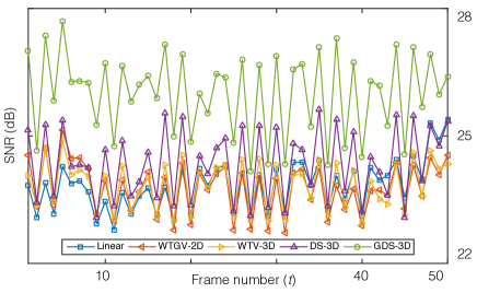
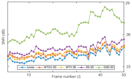
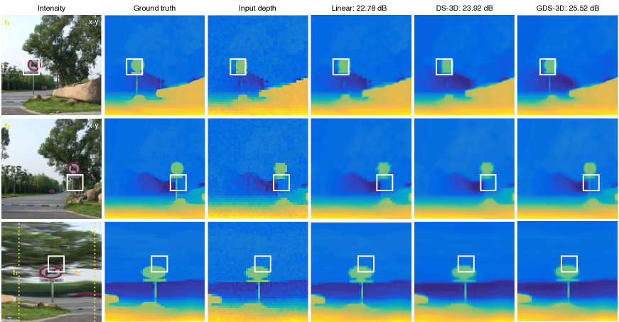
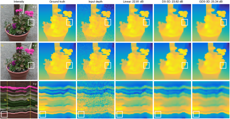
For quantitative comparison of the algorithms, we rely on the data-set by Zhang et al. [31], which consists of three video sequences Flower, Lawn, and Road, containing both intensity and depth information on the scenes. We considered images of size $128\times 128$ with $50$ time frames. The ground truth depth was downsized by factors of $2$, $3$, $4$, and $5$, and was corrupted by additive Gaussian noise corresponding to SNR of $30$ dB. Table 1 reports the SNR of superresolved depth for all the algorithms and downsizing factors. Figures 4 and 5 illustrate the evolution of SNR against the frame number for Road and Flower, respectively, at downsizing factor of $3$. The effectiveness of the proposed approach can also be appreciated visually in Figs. 6 and 7.

For additional validation, we test the algorithm on the KITTI dataset [32]. The dataset contains intensity images from PointGray Flea2 cameras and 3D point clouds from a Velodyne HDL-64E, which have been calibrated a priori using specific known targets. We consider a region of interest of $192\times 512$ pixels with $64$ time frames. The $495588$ total lidar measurements are randomly and uniformly split into a reconstruction and a validation sets. Note that this implies a depth measurement rate of just $3.94\%$. We then estimate depth from the reconstruction set using WTV-3D, as well as GDS-3D, and use the validation set to evaluate the quality of the results; these are illustrated in Fig. 8.

The examples and simulations in this section, validate our claim: the quality of estimated depth can be considerably boosted by properly incorporating temporal information into the reconstruction procedure. Comparison of GDS-2D against GDS-3D highlights the importance of additional temporal information. The approach we propose is implicitly motion adaptive and can thus preserve temporal edges substantially better than alternative approaches such as WTV-3D. Moreover, comparison between DS-3D and GDS-3D highlights that the usage of intensity significantly improves the performance of the algorithm. Note also the slight improvement in SNR of GDS-3D over ADMM-3D. This is consistent with the arguments in [29] that suggest to decouple data-fidelity from the enforcement of prior constraints when using block-matching-based methods.

5 Conclusion

We presented a novel motion-adaptive approach for guided superresolution of depth maps. Our method identifies and groups similar patches from several frames, which are then supperresolved using a rank regularizer. Using this approach, we can produce high-resolution depth sequences from significantly down-sized low-resolution ones. Compared to the standard techniques, the proposed method preserves temporal edges in the solution and effectively mitigates noise in practical configurations.

While our formulation has higher computational complexity than standard approaches that process each frame individually, it allows us to incorporate a very effective regularization for stabilizing the inverse problem associated with superresolution. The algorithms we describe enable efficient computation and straightforward implementation by reducing the problem to a succession of straightforward operations. Our experimental results demonstrate the considerable benefits of incorporating time and motion adaptivity into inverse-problems for depth estimation.

References

- [1] J. Diebel and S. Thrun, “An application of markov random ffield to range sensing,” in Proc. Advances in Neural Information Processing Systems 18, vol. 18, Vancouver, BC, Canada, December 5-8, 2005, pp. 291–298.
- [2] J. Kopf, M. F. Cohen, D. Lischinski, and M. Uyttendaele, “Joint bilateral upsampling,” in ACM Trans. Graph. (Proc. SIGGRAPH 2007), vol. 26, San Diego, CA, USA, August 5-9, 2007, p. 96.
- [3] Q. Yang, R. Yang, J. Davis, and D. Nister, “Spatial-depth super resolution for range images,” in Proc. IEEE Conf. Computer Vision and Pattern Recognition (CVPR), Minneapolis, MN, USA, June 17-22, 2007, pp. 1–8.
- [4] D. Chan, H. Buisman, C. Theobalt, and S. Thrun, “A noise-aware filter for real-time depth upsampling,” in ECCV Workshop on Multicamera and Multimodal Sensor Fusion Algorithms and Applications, 2008.
- [5] M.-Y. Liu, O. Tuzel, and Y. Taguchi, “Joint geodesic upsampling of depth images,” in Proc. IEEE Conf. Computer Vision and Pattern Recognition (CVPR), Portland, OR, USA, June 23-28, 2013, pp. 169–176.
- [6] J. Dolson, J. Baek, C. Plagemann, and S. Thrun, “Upsampling range data in dynamic environments,” in Proc. IEEE Conf. Computer Vision and Pattern Recognition (CVPR), vol. 23, San Francisco, CA, USA, June 13-18, 2010, pp. 1141–1148.
- [7] K. He, J. Sun, and X. Tang, “Guided image filtering,” in Proc. ECCV, Hersonissos, Greece, September 5-11, 2010, pp. 1–14.
- [8] ——, “Guided image filtering,” IEEE Trans. Patt. Anal. and Machine Intell., vol. 35, no. 6, pp. 1397–1409, June 2013.
- [9] E. J. Candès, J. Romberg, and T. Tao, “Robust uncertainty principles: Exact signal reconstruction from highly incomplete frequency information,” IEEE Trans. Inf. Theory, vol. 52, no. 2, pp. 489–509, February 2006.
- [10] D. L. Donoho, “Compressed sensing,” IEEE Trans. Inf. Theory, vol. 52, no. 4, pp. 1289–1306, April 2006.
- [11] Y. Li, T. Xue, L. Sun, and J. Liu, “Joint example-based depth map super-resolution,” in Proc. IEEE Int. Con. Multi., Melbourne, VIC, Australia, July 9-13, 2012, pp. 152–157.
- [12] D. Ferstl, C. Reinbacher, R. Ranftl, M. Ruether, and H. Bischof, “Image guided depth upsampling using anisotropic total generalized variation,” in Proc. IEEE Conf. Computer Vision and Pattern Recognition (CVPR), Sydney, NSW, Australia, December 1-8, 2013, pp. 993–1000.
- [13] X. Gong, J. Ren, B. Lai, C. Yan, and H. Qian, “Guided depth upsampling via a cosparse analysis model,” in Proc. IEEE CVPR WKSHP, Columbus, OH, USA, June 23-28, 2014, pp. 738–745.
- [14] W. Huang, X. Gong, and M. Y. Yang, “Joint object segmentation and depth upsampling,” IEEE Signal Process. Lett., vol. 22, no. 2, pp. 192–196, February 2015.
- [15] S. Schouon, C. Theobalt, J. Davis, and S. Thrun, “LidarBoost: Depth superresolution for ToF 3D shape scanning,” in Proc. IEEE Conf. Computer Vision and Pattern Recognition (CVPR), Miami, FL, USA, June 20-25, 2009, pp. 343–350.
- [16] A. Buades, B. Coll, and J. M. Morel, “Image denoising methods. A new nonlocal principle.” SIAM Rev, vol. 52, no. 1, pp. 113–147, 2010.
- [17] K. Dabov, A. Foi, V. Katkovnik, and K. Egiazarian, “Image denoising by sparse 3-D transform-domain collaborative filtering,” IEEE Trans. Image Process., vol. 16, no. 16, pp. 2080–2095, August 2007.
- [18] Z. Yang and M. Jacob, “Nonlocal regularization of inverse problems: A unified variational framework,” IEEE Trans. Image Process., vol. 22, no. 8, pp. 3192–3203, August 2013.
- [19] A. Danielyan, V. Katkovnik, and K. Egiazarian, “BM3D frames and variational image deblurring,” IEEE Trans. Image Process., vol. 21, no. 4, pp. 1715–1728, April 2012.
- [20] B. Huhle, T. Schairer, P. Jenke, and W. Strasser, “Fusion of range and color images for denoising and resolution enhancement with a non-local filter,” Comput. Vis. Image Underst., vol. 114, no. 12, pp. 1336–1345, December 2010.
- [21] J. Park, H. Kim, Y.-W. Tai, M. S. Brown, and I. Kweon, “High quality depth map upsampling for 3D-TOF cameras,” in Proc. IEEE Int. Conf. Comp. Vis., Barcelona, Spain, November 6-13, 2011, pp. 1623–1630.
- [22] S. Lu, X. Ren, and F. Liu, “Depth enhancement via low-rank matrix completion,” in Proc. IEEE Conf. Computer Vision and Pattern Recognition (CVPR), Columbus, OH, USA, June 23-28, 2014, pp. 3390–3397.
- [23] M. Fazel, “Matrix rank minimization with applications,” Ph.D. dissertation, PhD thesis, Stanford University, 2002.
- [24] R. Chartrand, “Nonconvex splitting for regularized Low-Rank + Sparse decomposition,” IEEE Trans. Signal Process., vol. 60, no. 11, pp. 5810–5819, November 2012.
- [25] Y. Hu, S. G. Lingala, and M. Jacob, “A fast majorize-minimize algorithm for the recovery of sparse and low-rank matrices,” IEEE Trans. Image Process., vol. 21, no. 2, pp. 742–753, February 2012.
- [26] H. Yoon, K. S. Kim, D. Kim, Y. Bresler, and J. C. Ye, “Motion adaptive patch-based low-rank approach for compressed sensing cardiac cine MRI,” IEEE Trans. Med. Imag., vol. 33, no. 11, pp. 2069–2085, November 2014.
- [27] J. Nocedal and S. J. Wright, Numerical Optimization, 2nd ed. Springer, 2006.
- [28] S. Boyd, N. Parikh, E. Chu, B. Peleato, and J. Eckstein, “Distributed optimization and statistical learning via the alternating direction method of multipliers,” Foundations and Trends in Machine Learning, vol. 3, no. 1, pp. 1–122, 2011.
- [29] A. Danielyan, “Block-based collaborative 3-D transform domain modeing in inverse imaging,” Publication 1145, Tampere University of Technology, May 2013.
- [30] L. I. Rudin, S. Osher, and E. Fatemi, “Nonlinear total variation based noise removal algorithms,” Physica D, vol. 60, no. 1–4, pp. 259–268, November 1992.
- [31] L. Zhang, S. Vaddadi, H. Jin, and S. K. Nayar, “Multiple view image denoising,” in Proc. IEEE Conf. Computer Vision and Pattern Recognition (CVPR), Miami, FL, USA, June 20-25, 2009, pp. 1542–1549.
- [32] A. Geiger, P. Lenz, C. Stiller, and R. Urtasun, “Vision meets robotics: The KITTI dataset,” International Journal of Robotics Research, vol. 32, no. 11, pp. 1231–1237, November 2013.