NNLOPS accurate associated HW production

Abstract

We present a next-to-next-to-leading order accurate description of associated HW production consistently matched to a parton shower. The method is based on reweighting events obtained with the HW plus one jet NLO accurate calculation implemented in POWHEG, extended with the MiNLO procedure, to reproduce NNLO accurate Born distributions. Since the Born kinematics is more complex than the cases treated before, we use a parametrization of the Collins-Soper angles to reduce the number of variables required for the reweighting. We present phenomenological results at 13 TeV, with cuts suggested by the Higgs Cross Section Working Group.

1 Introduction

After the discovery of the Higgs boson in Run I Aad:2012tfa ; Chatrchyan:2012xdj , one of the main tasks of the ongoing LHC Run II is to perform accurate measurements of Higgs properties. This will be done by a thorough investigation of all Higgs production and decay modes. Higgs boson production in association with a boson (HV) is the third largest Higgs production mode and so far has been studied in Run I in different channels, including $b\bar{b}$ Aad:2014xzb ; Chatrchyan:2013zna , $WW^{*}$ TheATLAScollaboration:2013hia ; CMS:zwa , and $\tau\tau$ CMS:ckv . Furthermore, for Higgs production in association with a $Z$ boson, it has been used to set bounds on invisible Higgs decay modes Chatrchyan:2014tja . Because of the largest branching ratio of Higgs to bottom quarks, so far the best significance was found in this channel, by both ATLAS (1.4 $\sigma$ significance) and CMS (2.2 $\sigma$ significance). It is expected that these results will quickly improve in Run II, both because of the increased luminosity and the higher energy. Higgs to bottom quarks is notably difficult because of the very large QCD background from $g\to bb$, hence it was suggested that associated production is best studied in a boosted regime Butterworth:2008iy . When boosted cuts are applied this channel becomes one of the most promising places to constrain the bottom Yukawa coupling.

In ref. Brein:2003wg the inclusive HV ($V=W,Z$) cross section was computed at NNLO. In refs. Ferrera:2011bk ; Ferrera:2014lca a fully differential NNLO calculation of HV including all Drell-Yan type contributions has been presented. The impact of top-quark loops at this perturbative order has also been investigated in ref. Brein:2011vx . In ref. Ferrera:2013yga NLO corrections to the $H\to bb$ decay were combined with the NNLO corrections to the production. NLO electroweak corrections are also known Ciccolini:2003jy ; Denner:2011id and available in the public code HAWK Denner:2014cla . Recently, in ref. Campbell:2016jau a NNLO calculation of HV was presented, that includes both Drell-Yan type and top Yukawa contributions, and that includes decays of the vector bosons and of the Higgs boson to $b\bar{b},\gamma\gamma,WW^{*}$.

In ref. Ferrera:2011bk it was shown that, while NNLO corrections to the inclusive HW cross section are tiny, of the order of 1-2%, the impact of NNLO corrections can increase substantially at the LHC when cuts are imposed on the decay products or when jet-veto criteria are applied. Since a jet-veto can have a large impact on the size of higher-order corrections, it should be modelled as accurately as possible. In an NNLO calculation, however, a jet is made up of only one or two partons, and no large all-order logarithms are accounted for. Although in this particular case large logarithms can be resummed quite precisely (for instance using the approaches of refs. Banfi:2012jm or Becher:2014aya ), it is often very useful, and at times needed, to model such effects by means of a fully-differential simulation, where large logarithms are resummed (although with limited logarithmic accuracy) by a parton shower algorithm. The precision required for LHC studies also demands that at least the NLO corrections be included in such event generation tools, providing therefore predictions where NLO effects are matched to parton showers (NLOPS). Thanks to the various implementations of the MC@NLO Frixione:2002ik and POWHEG Nason:2004rx algorithms such tools are now routinely used by experimentalists and theorists.

More specifically, the QCD NLO calculation of associated Higgs production (HV) was matched to parton showers with the MC@NLO method Frixione:2005gz , and, more recently, also using POWHEG Luisoni:2013kna . Ref. Luisoni:2013kna also contains NLOPS results for $\textrm{HV}{}+1$ jet, and a merging of the HV and HV+jet NLOPS simulations, obtained with the so-called “Multiscale improved NLO” approach (MiNLO in the following). The MiNLO approach was formulated in ref. Hamilton:2012np and subsequently refined in ref. Hamilton:2012rf . In the latter work it was shown that for processes where a colorless system $X$ is produced in a hadronic collision, one can simulate with NLOPS accuracy both $X$ and $X+1$ jet production simultaneously, without introducing any external merging scale. In refs. Hamilton:2012rf ; Hamilton:2013fea it was then shown that with a merged generator of $X$ and $X+1$ jet, and the NNLO computation for $X$ production, one can build an NNLO+parton shower accurate generator (NNLOPS from now on) for $X$ production. This approach was used to build NNLOPS accurate generators for Higgs via gluon fusion Hamilton:2013fea and Drell Yan production Karlberg:2014qua . Recently, the MiNLO method was extended further Frederix:2015fyz so that the one can merge even three units of multiplicity while preserving NLO accuracy. The construction of these NNLOPS generators based on MiNLO relies on a reweighting which is differential in the variables describing the inclusive $X$-production Born phase space. For Higgs production this amounts to a one-dimensional reweighting in the Higgs rapidity, while for Drell Yan production a three-dimensional reweighting has been used.

In this paper, we use the aforementioned MiNLO-based approach to match the results obtained in ref. Luisoni:2013kna for $\textrm{HW}{}+1$ jet production, to the exact NNLO QCD computation of HW presented in ref. Ferrera:2011bk , thereby obtaining the first NNLOPS accurate results for HW production, including leptonic decays of the $W$ boson. We remind the reader that, as in ref. Ferrera:2011bk , we only include contributions where the Higgs boson is radiated off a vector boson: top Yukawa contributions, i.e. contributions from diagrams containing a top-quark loop radiating an Higgs boson, have not been included in this work. Since the Born phase-space for $H\ell\nu$ production involves six variables, one would need to carry out a six-dimensional reweighting, which is currently numerically unfeasible. We will describe in the core of the paper how we deal with this problem.

The paper is organized as follows. In Sec. 2 we outline our method, and discuss in particular the treatment of the multi-dimensional Born phase space. In Sec. 3 we give all details about our practical implementation. In Sec. 4 we validate our results, while in Sec. 5 we present phenomenological results with cuts suggested for the writeup of the fourth Higgs Cross Section working group report. We conclude in Sec. 6. In App. A we give few more details about the scale variation uncertainties of the results.

2 Outline of the method

The method we use in this work is based on achieving NNLOPS accuracy by reweighting Les Houches events produced by the MiNLO-improved POWHEG HW plus one jet generator (HWJ-MiNLO). Each event, with a given weight, contains a final state made of the colorless system (the Higgs boson and the lepton pair from the $W$ boson) and 1 or 2 additional light QCD partons. NNLOPS accuracy is obtained by an appropriate rescaling of the original weight associated to each event. As described in detail in refs. Hamilton:2013fea ; Karlberg:2014qua , the rescaling must be differential in the variables describing the Born kinematics of the colorless system. Concretely, for each event one computes the Born variables using the kinematics of the colourless partons in the event kinematics, as is. Using these observables, a rescaling factor for each weight is computed. In its simplest form, the rescaling factor can be written as

$${\cal W}(\Phi_{\scriptscriptstyle B}{})=\frac{\frac{d\sigma^{\textrm{NNLO}}}{d\Phi_{\scriptscriptstyle B}{}}}{\frac{d\sigma^{{\tt MiNLO}}}{d\Phi_{\scriptscriptstyle B}{}}}\,,$$ (1)

where $\frac{d\sigma^{\textrm{NNLO}}}{d\Phi_{\scriptscriptstyle B}{}}$ ($\frac{d\sigma^{{\tt MiNLO}}}{d\Phi_{\scriptscriptstyle B}{}}$) is a multi-differential distribution obtained at pure NNLO level (using HWJ-MiNLO events), and $\Phi_{\scriptscriptstyle B}{}$ denotes the Born phase space.

It is clear that, by construction, Born variables will be described with NNLO accuracy. Furthermore, since the HWJ-MiNLO is NLO accurate for distributions inclusive on all radiation, it is straightforward to prove (along the lines of the proofs presented in refs. Hamilton:2013fea ; Karlberg:2014qua ) that this rescaling does not spoil the NLO accuracy of HWJ-MiNLO generator. As a consequence of these two facts, after rescaling, one obtains full NNLO accuracy for HW.

One might worry that once events undergo a parton shower, the NNLO accuracy might be lost. It is however easy to see that this is not the case: the second emission is generated by POWHEG precisely in such a way as to preserve the NLO accuracy of 1-jet observables. Hence the first emission generated by the parton shower is the third one, i.e. the effect of the parton shower starts at ${\cal O}(\alpha_{s}^{3})$, and is therefore beyond NNLO.

In the present case, the Born kinematics is fully specified by six independent variables. For instance one can choose the rapidity of the HW-system ($y_{\scriptscriptstyle\textrm{HW}}{}$), the difference in rapidity between the Higgs and the $W$ boson ($\Delta y_{\scriptscriptstyle\textrm{HW}}{}$), the Higgs transverse momentum ($p_{t,\scriptscriptstyle\textrm{H}}{}$), the dilepton pair invariant mass ($m_{\scriptscriptstyle\ell\nu}{}$) and two angular variables. A convenient standard choice for the angular variables is to use the Collins-Soper angles Collins:1977iv defined as follows. One considers a boost from the laboratory frame to the rest frame of the $W$ boson (the ${\cal O}^{\prime}$ frame). Using the positive and negative rapidity beam momenta, respectively $p^{\prime}_{A}$ and $p^{\prime}_{B}$ in ${\cal O}^{\prime}$, one defines a $z$-axis in this frame such that it bisects the angle between $p^{\prime}_{A}$ and $-p^{\prime}_{B}$. One then introduces a transverse unit vector $\hat{q}_{T}$, orthogonal to the $z$ axis and lying in the ($p^{\prime}_{A},p^{\prime}_{B}$) plane, pointing away from $p^{\prime}_{A}+p^{\prime}_{B}$. The Collins-Soper angles are defined as the polar angle $\theta^{*}$ of the lepton momentum $l^{\prime}$ in ${\cal O}^{\prime}$ with respect to the $z$-axis ($\vec{l}^{\prime}\cdot\hat{z}=|l^{\prime}|\cos\theta^{*}$) and the azimuthal angle $\phi^{*}$ of $l^{\prime}$ ($\vec{l}^{\prime}\cdot\hat{q}_{T}=|l^{\prime}|\sin\theta^{*}\cos\phi^{*}$).

Since the decay of a massive spin one particle is at most quadratic in the lepton momentum $\vec{l}^{\prime}$ in the frame ${\cal O}^{\prime}$, one can parametrize the angular dependence in terms of the nine spherical harmonic functions $Y_{lm}(\theta^{*},\phi^{*})$ with $l\leq 2$ and $|m|\leq l$. This can be understood from the observation that the decay of a massive spin one particle is associated to 9 degrees of freedom (the spin-density matrix is a 3x3 matrix). One of these coefficients is then fixed by the normalisation of the cross section, so that eight independent coefficients are sufficient to parametrize the angular dependence. As it is done in the case of Drell-Yan, it is convenient to introduce the following parametrisation for the angular dependence,

$$\frac{d\sigma}{d\Phi_{\scriptscriptstyle B}{}} = \frac{d^{6}\sigma}{dy_{\scriptscriptstyle\textrm{HW}}{}\,d\Delta y_{\scriptscriptstyle\textrm{HW}}{}\,dp_{t,\scriptscriptstyle\textrm{H}}{}\,dm_{\scriptscriptstyle\ell\nu}{}\,d\cos\theta^{*}d\phi^{*}}$$ (2)

$$= \frac{3}{16\pi}\left(\frac{d\sigma}{d\Phi_{\scriptscriptstyle\textrm{HW}^{*}}}(1+\cos^{2}\theta^{*})+\sum_{i=0}^{7}A_{i}(\Phi_{\scriptscriptstyle\textrm{HW}^{*}})f_{i}(\theta^{*},\phi^{*})\right)\,,$$

where we introduced for simplicity the four dimensional phase space of the $\textrm{HW}{}^{*}$ system, $\Phi_{\scriptscriptstyle\textrm{HW}^{*}}=\{y_{\scriptscriptstyle\textrm{HW}}{},\Delta y_{\scriptscriptstyle\textrm{HW}}{},p_{t,\scriptscriptstyle\textrm{H}}{},m_{\scriptscriptstyle\ell\nu}{}\}$ and $\frac{d\sigma}{d\Phi_{\scriptscriptstyle\textrm{HW}^{*}}}$ corresponds to the fully differential cross section integrated just over the Collins-Soper angles. The functions $f_{i}(\theta^{*},\phi^{*})$ are essentially given by spherical harmonics

$$\begin{aligned} f_{0}(\theta^{*},\phi^{*})&=\left(1-3\cos^{2}\theta^{*}\right)/2\,,\qquad\\ f_{2}(\theta^{*},\phi^{*})&=(\sin^{2}\theta^{*}\cos 2\phi^{*})/2\,,\\ f_{4}(\theta^{*},\phi^{*})&=\cos\theta^{*}\,,\\ f_{6}(\theta^{*},\phi^{*})&=\sin 2\theta^{*}\sin\phi^{*}\,,\\ \end{aligned}\begin{aligned} f_{1}(\theta^{*},\phi^{*})&=\sin 2\theta^{*}\cos\phi^{*}\,,\\ f_{3}(\theta^{*},\phi^{*})&=\sin\theta^{*}\cos\phi^{*}\,,\\ f_{5}(\theta^{*},\phi^{*})&=\sin\theta^{*}\sin\phi^{*}\,,\\ f_{7}(\theta^{*},\phi^{*})&=\sin^{2}\theta^{*}\sin 2\phi^{*}\,.\end{aligned}$$ (3)

They have the property that their integral over the solid angle $d\Omega=d\cos\theta^{*}d\phi^{*}$ vanishes.

Since the angular dependence is fully expressed in terms of the $f_{i}(\theta^{*},\phi^{*})$ functions, the coefficients of the expansion $A_{i}(\Phi_{\scriptscriptstyle\textrm{HW}^{*}})$ are functions only of the remaining kinematical variables $\Phi_{\scriptscriptstyle\textrm{HW}^{*}}$. The coefficients $A_{i}(\Phi_{\scriptscriptstyle\textrm{HW}^{*}})$ can then be extracted using orthogonality properties of the spherical harmonics. We find

$$\begin{aligned} A_{0}(\Phi_{\scriptscriptstyle\textrm{HW}^{*}})&=4\,({d\sigma}/{d\Phi_{\scriptscriptstyle\textrm{HW}^{*}}})-\langle 10\cos^{2}\theta^{*}\rangle\,,\quad\\ A_{2}(\Phi_{\scriptscriptstyle\textrm{HW}^{*}})&=\langle 10\sin^{2}\theta^{*}\cos 2\phi^{*}\rangle\,,\quad\\ A_{4}(\Phi_{\scriptscriptstyle\textrm{HW}^{*}})&=\langle 4\cos\theta^{*}\rangle\,,\quad\\ A_{6}(\Phi_{\scriptscriptstyle\textrm{HW}^{*}})&=\langle 5\sin 2\theta^{*}\sin\phi^{*}\rangle\,,\quad\\ \end{aligned}\begin{aligned} A_{1}(\Phi_{\scriptscriptstyle\textrm{HW}^{*}})&=\langle 5\sin 2\theta^{*}\cos\phi^{*}\rangle\,,\\ A_{3}(\Phi_{\scriptscriptstyle\textrm{HW}^{*}})&=\langle 4\sin\theta^{*}\cos\phi^{*}\rangle\,,\\ A_{5}(\Phi_{\scriptscriptstyle\textrm{HW}^{*}})&=\langle 4\sin\theta^{*}\sin\phi^{*}\rangle\,,\\ A_{7}(\Phi_{\scriptscriptstyle\textrm{HW}^{*}})&=\langle 5\sin^{2}\theta^{*}\sin 2\phi^{*}\rangle\,,\end{aligned}$$ (4)

where the expectation values $\langle f(\theta^{*},\phi^{*})\rangle$ are functions of $\Phi_{\scriptscriptstyle\textrm{HW}^{*}}$ defined as

$$\langle f(\theta^{*},\phi^{*})\rangle=\int{d\cos\theta^{*}d\phi^{*}}\frac{d\sigma}{d\Phi_{\scriptscriptstyle B}{}}f(\theta^{*},\phi^{*})\,.$$ (5)

Hence, in order to compute both the numerator and denominator in eq. (1), as required for the reweighting, we can use eq. (2) with the angular functions defined in eq. (3) and the coefficients computed using eq. (4). In summary, by using the Collins-Soper angles one can turn the problem of computing differential distributions in six variables, into the determination of nine four-dimensional distributions, i.e. $d\sigma/d\Phi_{\scriptscriptstyle\textrm{HW}^{*}}$ and the eight distributions $A_{i}(\Phi_{\scriptscriptstyle\textrm{HW}^{*}})$ of eq. (4).

3 Practical implementation

In the previous section we have outlined the method that we will use in the following to achieve NNLOPS accuracy. Here, we will provide details about the choices that we made in our practical implementation, we outline the setup that we have adopted to present the results of this paper, and we give the procedure that we used to estimate the theoretical uncertainty.

3.1 Procedure

A first consideration is that when using multi-differential distributions one needs to decide the number of bins in each distribution. Previous experience suggests that having about 25 bins per direction is sufficient for practical purposes, hence we will adopt this choice here. In order to improve the numerical precision, we find it useful to use bins that contain approximately the same cross-section, as opposed to bins that are equally spaced. Practically, we perform (moderate statistics) warm-up runs at NLO using HWJ-MiNLO. From the differential cross sections obtained from these runs, we determine the appropriate bins. We then read in the bin values when performing high-statistic runs to extract the needed distributions.

We have simplified our procedure by noting that the $m_{\scriptscriptstyle\ell\nu}{}$ invariant mass distribution has a flat $K$-factor. This is true even when examining the $d\sigma/d{m_{\scriptscriptstyle\ell\nu}{}}$ distribution in different bins of $\Phi_{\scriptscriptstyle\textrm{HW}}=\{y_{\scriptscriptstyle\textrm{HW}}{},\Delta y_{\scriptscriptstyle\textrm{HW}}{},p_{t,\scriptscriptstyle\textrm{H}}{}\}$. Therefore, in eq. (2) we replace $\Phi_{\scriptscriptstyle\textrm{HW}^{*}}$ with $\Phi_{\scriptscriptstyle\textrm{HW}}$ and in eq. (5) we integrate over $m_{\ell\nu}$, meaning that instead of having four-dimensional distributions, we use three-dimensional ones. This is an approximation, however we believe that it works extremely well, as discussed in Sec. 4.

A further point to note is that, as observed already in ref. Hamilton:2013fea , a reweighting of the form eq. (1) spreads the NNLO/NLO $K$-factor uniformly, even in regions where the HW system has a large transverse momentum, i.e. a region that is described equally well by a pure NNLO HW calculation, or by the HWJ-MiNLO generator. However, it is also possible to introduce a reweighting that goes smoothly to one in the regions where both generators have the same accuracy to start with. In order to do this, one introduces a smooth function of $p_{\scriptscriptstyle T}$, that goes to one at $p_{\scriptscriptstyle T}=0$ and that vanishes at infinity. For instance, one can introduce

$$h(p_{\scriptscriptstyle T})=\frac{(M_{\scriptscriptstyle H}+M_{\scriptscriptstyle W})^{2}}{(M_{\scriptscriptstyle H}+M_{\scriptscriptstyle W})^{2}+p_{\scriptscriptstyle T}^{\;2}}\,,$$ (6)

to split the cross-section into

$$d\sigma_{\scriptscriptstyle A}=d\sigma\,h(p_{\scriptscriptstyle T})\,,\qquad d\sigma_{\scriptscriptstyle B}=d\sigma\,(1-h(p_{\scriptscriptstyle T}))\,.$$ (7)

One then reweights the HWJ-MiNLO events using

$$\mathcal{W}\left(\Phi_{\scriptscriptstyle\textrm{HW}},\,p_{{\scriptscriptstyle\mathrm{T}}}\right) = h\left(p_{\scriptscriptstyle\mathrm{t}}\right)\,\frac{\smallint d\sigma^{{\scriptscriptstyle\mathrm{NNLO\phantom{i}}}}\,\delta\left(\Phi_{\scriptscriptstyle\textrm{HW}}-\Phi_{\scriptscriptstyle\textrm{HW}}\left(\Phi\right)\right)-\smallint d\sigma_{\scriptscriptstyle B}^{{\scriptscriptstyle\mathrm{{\tt MiNLO}}}}\,\delta\left(\Phi_{\scriptscriptstyle\textrm{HW}}-\Phi_{\scriptscriptstyle\textrm{HW}}\left(\Phi\right)\right)}{\smallint d\sigma_{\scriptscriptstyle A}^{{\scriptscriptstyle\mathrm{{\tt MiNLO}}}}\,\delta\left(\Phi_{\scriptscriptstyle\textrm{HW}}-\Phi_{\scriptscriptstyle\textrm{HW}}\left(\Phi\right)\right)}$$ (8)

$$+ \left(1-h\left(p_{\scriptscriptstyle\mathrm{t}}\right)\right)\,.$$

This reweighting factor preserves the exact value of the NNLO differential cross-section

$$\left(\frac{d\sigma}{d\Phi_{\scriptscriptstyle\textrm{HW}}}\right)^{{\scriptscriptstyle\mathrm{NNLOPS}}} = \left(\frac{d\sigma}{d\Phi_{\scriptscriptstyle\textrm{HW}}}\right)^{{\scriptscriptstyle\mathrm{NNLO}}}\,.$$ (9)

We choose $p_{\scriptscriptstyle T}$ to be the transverse momentum of the leading jet when clustering events with the inclusive $k_{T}$-algorithm with $R=0.4$ Catani:1993hr ; Ellis:1993tq . The reason for this is choice is that $h(p_{T})$ goes to one when no radiation is present, since the leading jet transverse momentum vanishes. On the contrary, when hard radiation is present, the transverse momentum of the leading jet becomes large, $h(p_{T})$ goes to zero, and accordingly ${\cal W}(\Phi_{\scriptscriptstyle\textrm{HW}},p_{\scriptscriptstyle T})$ goes to one.

3.2 Settings

We give here a complete description of the setup used for the results presented in this paper. The specific process studied is

$$pp\longrightarrow HW^{+}\longrightarrow H\ell^{+}\nu_{\ell}\,,$$ (10)

where $\ell^{+}=\{e^{+},\mu^{+}\}$. We note that we leave the Higgs boson in the final state, rather than decaying it.

We used the code HVNNLO hvnnlo to obtain NNLO predictions, and the HWJ-MiNLO code Luisoni:2013kna implemented in the POWHEG BOX Alioli:2010xd to produce Les Houches events. Throughout this work we consider 13 TeV LHC collisions and use the MMHT2014nnlo68cl parton distribution functions Harland-Lang:2014zoa , corresponding to a value of $\alpha_{s}(M_{Z})=0.118$. We set $M_{W}=80.399$ GeV and $\Gamma_{W}=2.085$ GeV. Furthermore we use $\alpha_{\rm em}=1/132.3489$ and $\sin^{2}\theta_{W}=0.2226$. Finally we use $M_{H}=125$ GeV. Jets have been constructed using the anti-$k_{t}$ algorithm with $R=0.4$ Cacciari:2008gp as implemented in FastJet Cacciari:2005hq ; Cacciari:2011ma . For HWJ-MiNLO events the scale choice is dictated by the MiNLO procedure; for the NNLO we have used for the central renormalisation and factorisation scales $\mu_{0}=M_{H}+M_{W}$.

To shower partonic events we have used Pythia8 Sjostrand:2007gs (version 8.185) with the “Monash 2013” Skands:2014pea tune. To define leptons from the boson decays we use the Monte Carlo truth, i.e. we assume that if other leptons are present, the ones coming from the $W$ decay can be identified correctly. To obtain the results shown in the following sections, we have switched on the “doublefsr” option introduced in ref. Nason:2013uba . The plots shown throughout the paper have been obtained keeping the veto scale equal to the default POWHEG prescription.

3.3 Estimating uncertainties

We outline here the procedure that we use to estimate the uncertainties in our NNLOPS event generator. This procedure is similar to the one already used in refs. Hamilton:2013fea ; Karlberg:2014qua , but we find it useful to recall it here for completeness. As is standard, the uncertainties in the HWJ-MiNLO generator are obtained by varying by a factor 2 up and down independently all renormalisation scales appearing in the MiNLO procedure by $K_{\scriptscriptstyle\mathrm{R}}$ (simultaneously) and the factorisation scale by $K_{\scriptscriptstyle\mathrm{F}}$, keeping $1/2\leq K_{\scriptscriptstyle\mathrm{R}}/K_{\scriptscriptstyle\mathrm{F}}\leq 2$. This leads to 7 different scale choices given by

$$(K_{\scriptscriptstyle\mathrm{R}},K_{\scriptscriptstyle\mathrm{F}})=(0.5,0.5),(1,0.5),(0.5,1),(1,1),(2,1),(1,2),(2,2)\,\text{.}$$ (11)

The seven scale variation combinations have been obtained by using the reweighting feature of the POWHEG BOX.

For the pure NNLO results the uncertainty band is the envelope of the same 7-scale variations as used for HWJ-MiNLO uncertainties. Currently, in the next-to-next-to-leading order computation in HVNNLO, the only way of doing scale variations is to re-run the entire program with new scales. To be more efficient, one can instead compute the NNLO result at just 3 scale choices for $\mu_{F}$, e.g. $(K_{\scriptscriptstyle\mathrm{R}},K_{\scriptscriptstyle\mathrm{F}})=(1,0.5),(1,1),(1,2)$, along with pure LO and NLO results. One can then use renormalisation group equations to predict results at different renomalization scales.

For the NNLOPS results, we have first generated a single HWJ-MiNLO event file with all the weights needed to compute the integrals $d\sigma_{A/B}^{\scriptscriptstyle\mathrm{MINLO}}/d\Phi_{\scriptscriptstyle B}{}$ entering eq. (8) for all 7 scale choices.

The differential cross-section $d\sigma^{\scriptscriptstyle\mathrm{NNLO}}/d\Phi$ was tabulated for each of the seven scale variation points corresponding to $1/2\leq K_{\scriptscriptstyle\mathrm{R}}^{\prime}/K_{\scriptscriptstyle\mathrm{F}}^{\prime}\leq 2$. The analysis is then performed by processing the MiNLO event for given values of $(K_{\scriptscriptstyle\mathrm{R}},K_{\scriptscriptstyle\mathrm{F}})$, and multiplying its weight with the factor

$$h\left(p_{\scriptscriptstyle\mathrm{t}}\right)\times\,\frac{\smallint d\sigma_{(K_{\scriptscriptstyle\mathrm{R}}^{\prime},K_{\scriptscriptstyle\mathrm{F}}^{\prime})}^{{\scriptscriptstyle\mathrm{NNLO\phantom{i}}}}\,\delta\left(\Phi_{\scriptscriptstyle B}{}-\Phi_{\scriptscriptstyle B}{}(\Phi)\right)-\smallint d\sigma_{B,(K_{\scriptscriptstyle\mathrm{R}},K_{\scriptscriptstyle\mathrm{F}})}^{{\scriptscriptstyle{\tt MiNLO}}}\,\delta\left(\Phi_{\scriptscriptstyle B}{}-\Phi_{\scriptscriptstyle B}{}(\Phi)\right)}{\smallint d\sigma_{A,(K_{\scriptscriptstyle\mathrm{R}},K_{\scriptscriptstyle\mathrm{F}})}^{{\scriptscriptstyle{\tt MiNLO}}}\,\delta\left(\Phi_{\scriptscriptstyle B}{}-\Phi_{\scriptscriptstyle B}{}(\Phi)\right)}+\left(1-h\left(p_{\scriptscriptstyle\mathrm{t}}\right)\right)\,.$$ (12)

The central value is obtained by setting $(K_{\scriptscriptstyle\mathrm{R}},K_{\scriptscriptstyle\mathrm{F}})=(K_{\scriptscriptstyle\mathrm{R}}^{\prime},K_{\scriptscriptstyle\mathrm{F}}^{\prime})=(1,1)$, while to obtain the uncertainty band we apply this formula for all the seven $(K_{{\scriptscriptstyle\mathrm{R}}},K_{{\scriptscriptstyle\mathrm{F}}})$ and seven $(K_{{\scriptscriptstyle\mathrm{R}}}^{\prime},K_{{\scriptscriptstyle\mathrm{F}}}^{\prime})$ choices. This yields 49 scale variations in the final NNLOPS accurate events.

As explained in refs. Hamilton:2013fea ; Karlberg:2014qua , the motivation to vary scales in the NNLO and HWJ-MiNLO results independently is that, in the same spirit of the efficiency method Banfi:2012yh , we regard uncertainties in the overall normalisation of distributions as being independent of the respective uncertainties in the shapes.

4 Validation

4.1 Validation of the NNLOPS method

Our method uses the approximation that the $K$-factor of the dilepton system invariant mass is flat in the whole phase space. Hence, we first discuss how good this approximation is.

Figure 1 (left)

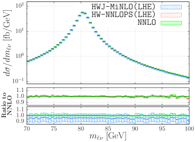
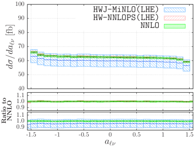
Figure 1: Comparison of HWJ-MiNLO(LHE) (blue), NNLO (green) and HW-NNLOPS(LHE) (red) for $m_{\scriptscriptstyle\ell\nu}{}$ (left) and $a_{\scriptscriptstyle\ell\nu}{}$ (right) defined in eq. (13).

shows the distribution of the $(l,\nu)$-invariant mass $m_{\ell\nu}$ integrated over the whole phase space. The right plot shows the distribution of

$$a_{\scriptscriptstyle\ell\nu}{}=\arctan\left(\frac{m_{\scriptscriptstyle\ell\nu}{}-m_{W}}{m_{W}\Gamma_{W}}\right)$$ (13)

which is constructed in order to flatten the $m_{\scriptscriptstyle\ell\nu}{}$ distribution. The upper panels show the predictions from HWJ-MiNLO(LHE) at pure Les Houches event (LHE) level, i.e. including NLO and Sudakov effects, but prior to parton shower (blue), predictions at HW-NNLOPS(LHE) level, i.e. including NNLO corrections and Sudakov effects but no parton shower (red) and NNLO results (green). The lower panels show the ratio to the NNLO result. The uncertainty bands are computed as described in Sec. 3.3. We notice that NNLO and HW-NNLOPS(LHE) predictions agree very well within their small uncertainty bands. HWJ-MiNLO(LHE) predictions are about 5% lower, but, as expected, the NNLO/NLO $K$-factor is flat over the whole region. In fact, the distributions have a Breit-Wigner shape, hence one expects higher-order corrections to affect the shape only very mildly, if at all.

Since our reweighting procedure is differential in all Born variables, but for $m_{\scriptscriptstyle\ell\nu}{}$, we need to also verity that the NNLO/NLO $K$-factor is flat in bins of all other Born variables. This is equivalent to saying that the NNLO/NLO $K$-factors for all other Born variables should be the same in every bin in $m_{\scriptscriptstyle\ell\nu}$ (or equivalently in $a_{\scriptscriptstyle\ell\nu}{}$). In Fig. 2 (left)

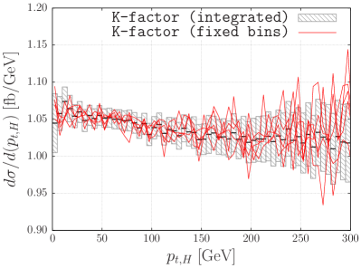
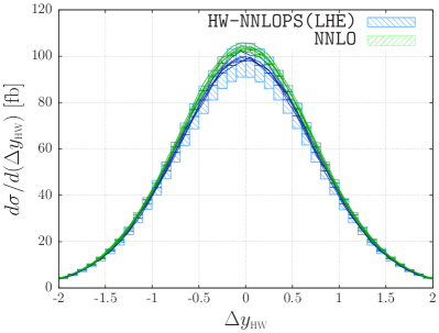
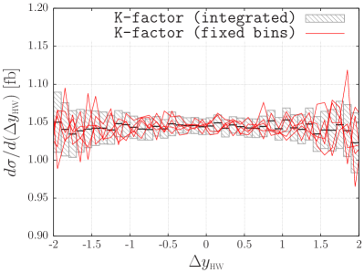
Figure 2: Comparison of HWJ-MiNLO(LHE) (blue) and NNLO (green) for Born variables $\Phi_{\scriptscriptstyle\textrm{HW}}$ chosen to perform reweighting. Left-panel: boxes represent results integrated over whole phase space (with theoretical uncertainty), whereas lines come from various $a_{\scriptscriptstyle\ell\nu}{}$ bins (as described in the text). Right-panel: boxes represent the overall $K$-factor (integrated over $a_{\scriptscriptstyle\ell\nu}{}$) with statistical uncertainty, while lines represent $K$-factors corresponding to various $a_{\scriptscriptstyle\ell\nu}{}$ bins (bin 3, 8, 13, 18, 23).

we show the comparison between HWJ-MiNLO(LHE) and NNLO for the three Born variables $y_{\scriptscriptstyle\textrm{HW}}{}$, $p_{t,\scriptscriptstyle\textrm{H}}{}$ and $\Delta y_{\scriptscriptstyle\textrm{HW}}{}$. Here the blue and green bands represent the usual theoretical uncertainty. In the right panels the black line shows the $K$-factor integrated over the whole $a_{\scriptscriptstyle\ell\nu}{}$ range and the five red lines show the same $K$-factor in a fixed $a_{\scriptscriptstyle\ell\nu}{}$ bin. Now, the grey band corresponds to the statistical uncertainty of the $K$-factor integrated over the whole $a_{l\nu}$ range, multiplied by a factor 5. Since we are probing 25 bins in $a_{\scriptscriptstyle\ell\nu}{}$, one expects that the statistical uncertainty for a particular bin is bigger by $\sqrt{N_{\textrm{bins}}}$ (we recall that the $a_{\scriptscriptstyle\ell\nu}{}$ distribution is by construction fairly flat). Therefore this band provides an estimate of the uncertainty of the $K$-factor on each $a_{\scriptscriptstyle\ell\nu}{}$ bin. We see that, within statistical fluctuations, the red lines lie within the grey band. This shows that, within the statistical uncertainties, the $K$-factor is independent of the value of $a_{\scriptscriptstyle\ell\nu}{}$.

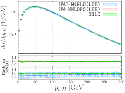
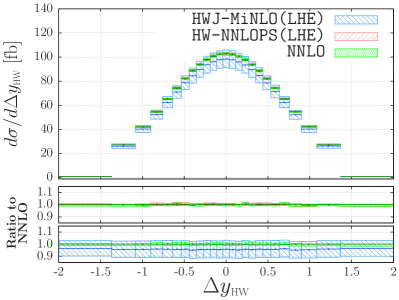
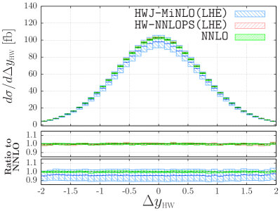
Figure 3: Comparison of HWJ-MiNLO(LHE) (blue), HW-NNLOPS(LHE) (red) and NNLO (green) predictions for the Born variables $\Phi_{\scriptscriptstyle\textrm{HW}}$ chosen to perform reweighting. Left panels show rebinned distributions (used for reweighting), right panels show differential distributions with equispaced bins.

For further validation we should check whether the distributions of the Born variables $\Phi_{\scriptscriptstyle\textrm{HW}}$ obtained with HW-NNLOPS(LHE) reproduce the results from the HVNNLO code. In Fig. 3 we can see rebinned distributions that we have used for reweighting (left) and unrebinned distributions (right) of the rapidity of the HW system $y_{\scriptscriptstyle\textrm{HW}}{}$, the transverse momentum of Higgs boson $p_{t,\scriptscriptstyle\textrm{H}}{}$ and the rapidity difference between Higgs and W-boson $\Delta y_{\scriptscriptstyle\textrm{HW}}{}$. We see that in the rebinned distributions we find perfect agreement between HW-NNLOPS(LHE) and NNLO results. For the unrebinned distributions we see that, when rebinned bins are large, e.g. for $|y_{\scriptscriptstyle\textrm{HW}}{}|\gtrsim 3$, minor artifacts are present. These can be always reduced using a suitable, finer binning for the 3D-histograms used for the reweighting.

As expected, the HW-NNLOPS(LHE) results reproduce very well results from HVNNLO and the uncertainty band of HWJ-MiNLO(LHE) shrinks from around $\pm 10\%$ to about $\pm 2\%$ in the HW-NNLOPS(LHE) case, which is a result of including NNLO corrections.

4.2 Validation of the use of Collins-Soper angles

As discussed in the previous section the Collins-Soper (CS) frame is a natural choice for the description of spin one vector boson decay. This frame is convenient since it allows the angular dependence of the vector decay to be parametrized in terms of only eight coefficients. Here we want to verify how well the CS parametrization works in practice.

In the case of $\theta^{*}$ distributions the only terms in Eq. (2) that contribute are $A_{0}$ and $A_{4}$, since the other terms drop out when integrating over $\phi^{*}$. The $\phi^{*}$ distributions on the other hand depend only on $A_{2},A_{3},A_{5}$ and $A_{7}$.

In the upper left panel of Fig. 4 we show the dependence of the coefficient $A_{4}$ on $y_{\scriptscriptstyle\textrm{HW}}{}$, whereas in the upper right plot we present the $\theta^{*}$ distribution integrated over the whole range of $p_{t,\scriptscriptstyle\textrm{H}}{}$, $\Delta y_{\scriptscriptstyle\textrm{HW}}{}$ and, as an example, in the range of $y_{\scriptscriptstyle\textrm{HW}}{}$ marked on the left upper plot by a yellow band. The red and green bands denote the theoretical uncertainty, as described before. The orange line shows the prediction from Eq. (2) with the coefficients computed for the central scale choice from Eq. (4) at pure NNLO level. Notice that the $\theta^{*}$ distribution is not symmetric since we have restricted ourselves to $y_{\scriptscriptstyle\textrm{HW}}$ values where $A_{4}$ is always positive, hence the functional dependence encoded in $f_{4}(\theta^{*},\phi^{*})$ is visible. From the r.h.s. plot we can see that the central NNLO result is fully compatible with $f(\theta^{*})$, i.e. the prediction from Eq. (2). Furthermore, we see that the NNLO prediction is consistent with the HW-NNLOPS(LHE) one, both for the central scale and for the scale variation, as was the case for the other Born variables used for reweighting.

Similar considerations apply to the $\phi^{*}{}$ dependence, whose shape is determined by the $A_{i}$ coefficients, as the first term in Eq. (2) integrates to a constant factor. We show in the lower left panel of Fig. 4 the dependence of the coefficient $A_{2}$ on $p_{t,\scriptscriptstyle\textrm{H}}{}$ while integrated over the remaining variables. In the lower right plot we display the distribution of $\phi^{*}$ integrated over whole range of $y_{\scriptscriptstyle\textrm{HW}}{}$ and $\Delta y_{\scriptscriptstyle\textrm{HW}}{}$, but restricted to the $p_{t,\scriptscriptstyle\textrm{H}}{}$ interval highlighted with a yellow band in the left plot. As for the $\theta^{*}$ distribution, we have good agreement between the HW-NNLOPS(LHE) result and the differential cross section reconstructed from the CS parametrization. As expected, the NNLO prediction is also consistent with the HW-NNLOPS(LHE) one.

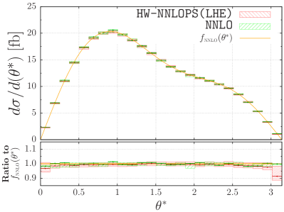
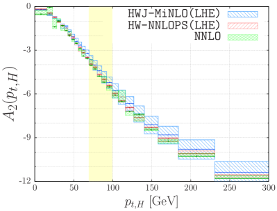
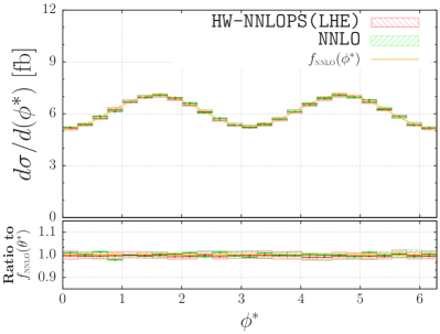
Figure 4: Upper panel: The left plot shows the $A_{4}$ coefficient as a function of $y_{\scriptscriptstyle\textrm{HW}}{}$. The right plot shows the distribution of $\theta^{*}$ integrated over all variables with $y_{\scriptscriptstyle\textrm{HW}}{}$ restricted to the region marked as yellow band in the left panel. Lower panel: The left plot shows the $A_{2}$ coefficient as a function of $p_{t,\scriptscriptstyle\textrm{H}}{}$. The right plot shows the distribution of $\phi^{*}$ integrated over all variables with $p_{t,\scriptscriptstyle\textrm{H}}{}$ restricted to the region marked as yellow band in the left panel.

These and similar plots validate our use of the extraction of the $A_{i}$ coefficients and their use to parametrize the angular dependence.

5 Phenomenological results

We will now discuss a few phenomenological results obtained with our new code. We remind the reader that the specific process studied here is $pp\rightarrow H\ell^{+}\nu_{\scriptscriptstyle\ell}$, with $\ell^{+}=\{e^{+},\mu^{+}\}$ and that we do not consider decays of the Higgs boson.

For all the results presented in this section we apply the cuts that were suggested in the context of the Higgs Cross Section Working Group (HXSWG) activity for the preparation of the fourth Yellow Report. We consider $13$ TeV LHC collisions. We require one positively charged lepton with $|y_{\ell}|<2.5$ and $p_{t,\ell}>15$ GeV, while we do not impose a missing energy cut. When applying a jet-cut or a jet-veto we define a jet as having $p_{t,j}>20$ GeV and $|y_{j}|<4.5$. Jets are reconstructed using the anti-$k_{t}$ algorithm Cacciari:2008gp with $R=0.4$, as implemented in Fastjet Cacciari:2011ma . At the moment we do not apply any cuts on the Higgs boson, however our code produces Les Houches events, which can be interfaced with any tool that provides the decay of the Higgs in the narrow width approximation. For example, this can be obtained easily by allowing Pythia8 to treat the Higgs boson as an unstable object.

5.1 Fiducial cross-section

The fiducial cross section at $\sqrt{s}=13$ TeV, together with its theoretical uncertainty, at different levels of the simulation, is given in table 1. From these results we obtain a $K$-factor between HVNNLOPS and HWJ-MiNLO equal to $1.04$.

	HWJ-MiNLO	HVNNLO	HVNNLOPS
$\sigma_{tot}$	$\quad 152.49(5)\;$fb$\>\pm 7.0\%\quad$	$\quad 158.75(8)\;$fb$\>\pm 1.0\%\quad$	$\quad 159.21(30)\;$fb$\>\pm 1.0\%\quad$

Table 1: Fiducial cross-section of $pp\rightarrow HW^{+}\rightarrow H\ell^{+}\nu_{\ell}$ at $\sqrt{s}=13$ TeV with leptonic cuts. The uncertainty band is obtained with the scale variation procedure described in the text. Numerical errors for each prediction are quoted in brackets, and relative details are given in the text.

We also see that the reweighting procedure of HWJ-MiNLO events to NNLOPS accuracy gives a result compatible with the fixed order NNLO calculation. In particular, the sizes of scale uncertainties for the HVNNLOPS and HVNNLO results are fully comparable, providing a reduction of almost one order of magnitude with respect to the HWJ-MiNLO result. The number quoted in bracket for the HWJ-MiNLO and HVNNLO results is the statistical error, and it is entirely due to Monte Carlo integration. The HVNNLOPS statistical uncertainty was found to be compatible with the one of HWJ-MiNLO. The numerical error quoted for the HVNNLOPS result is larger because it also contains a systematic component, that we added in quadrature to the statistical one, and which is due to bin-size effects in the reweighting procedure.

5.2 Higgs and Leptonic Observables

In the following we consider cross-sections obtained at various levels: at Les Houches event level before shower at NLO or NNLO accuracy, HWJ-MiNLO(LHE) and HW-NNLOPS(LHE), respectively; after showering the HWJ-MiNLO(LHE) and HW-NNLOPS(LHE) events with Pythia8, HWJ-MiNLO(Pythia8) and HW-NNLOPS(Pythia8), both with and without hadronization.

We start by showing in Fig. 5 the distributions for the transverse momenta of the $W$ boson and the HW system, respectively.

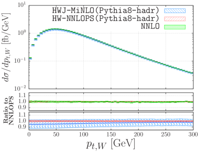
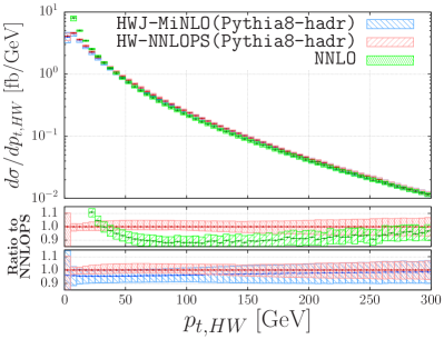
Figure 5: Comparison of HWJ-MiNLO (blue), NNLO (green), and HW-NNLOPS (red) predictions for $p_{\scriptscriptstyle\mathrm{t,W}}$ (left) and $p_{\scriptscriptstyle\mathrm{t,HW}}$ (right).

NNLO results are compared against those obtained with HWJ-MiNLO and HVNNLOPS. For observables that are fully inclusive over QCD radiation, such as $p_{\scriptscriptstyle\mathrm{t,W}}$, the agreement among the HVNNLO and NNLOPS predictions is perfect, as expected. As in the case of the fiducial cross-section one notices the sizable reduction of the uncertainty band from around $7$% in HWJ-MiNLO to about $1\%$ in the case of HVNNLO and HVNNLOPS. As no particularly tight cuts are imposed, the NNLO/NLO $K$-factor is almost exactly flat.

The right panel shows instead the effects due to the Sudakov resummation. At small transverse momenta, the NNLO cross section becomes larger and larger due to the singular behaviour of the matrix elements for HW production in association with arbitrarily soft-collinear emissions. The MiNLO method resums the logarithms associated to these emissions, thereby producing the typical Sudakov peak, which for this process is located at $2\text{ GeV }\nobreak\lesssim\nobreak p_{\scriptscriptstyle\mathrm{t,HW}}\lesssim 5\text{ GeV}$, as expected from the fact that the LO process is Drell-Yan like. It is also interesting to notice here two other features that occur away from the collinear singularity, and which are useful to understand the plots which are shown later. Firstly, the $p_{\scriptscriptstyle\mathrm{t}}$-dependence of the NNLO reweighting can be explicitly seen in the bottom panel, where one can also appreciate that at very large values not only the NNLOPS and MiNLO results approach each other, but also that the uncertainty band of HVNNLOPS becomes progressively larger (in fact, in this region, the nominal accuracy is NLO). Secondly, in the region $30\text{ GeV}\nobreak\lesssim\nobreak p_{\scriptscriptstyle\mathrm{t,HW}}\nobreak\lesssim\nobreak 250\nobreak\text{ GeV}$, the NNLO and NNLOPS lines show deviations of up to $10$ %: these are due to both the compensation that needs to take place in order for the two results to integrate to the same total cross section, and the fact that the scale choices are different (fixed for the NNLO line, dynamic and set to $p_{\scriptscriptstyle\mathrm{t,HW}}$ in MiNLO). When $p_{\scriptscriptstyle\mathrm{t,HW}}\gtrsim 250$ GeV the two predictions start to approach, as this is the region of phase space where the MiNLO scale is similar to that used at NNLO ($\mu=M_{\scriptscriptstyle H}+M_{\scriptscriptstyle W}$). At even higher transverse momenta, $p_{\scriptscriptstyle\mathrm{t,HW}}\gtrsim 400$ GeV, the MiNLO Sudakov is not active, however the MiNLO scale is set to the transverse momentum which is higher than the scale in the NNLO calculation. As consequence, the NNLOPS results are lower than the NNLO one.

It is interesting to look at a variable describing the decay of the HW resonance, e.g. the azimuthal angle between the $W^{+}$ boson and the Higgs particle ($\Delta\phi_{\textrm{HW}}$). At leading order the two particles are back-to-back, $\Delta\phi_{\textrm{HW}}=\pi$, but real radiation moves the bosons away from this configuration. In Fig. 6 (left) we show the distribution of $\Delta\phi_{\textrm{HW}{}}$ comparing the HVNNLO result to the result of our simulation after including parton shower effects, before and after the NNLO rescaling.

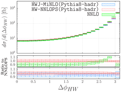
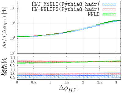
Figure 6: Azimuthal angle between the Higgs boson and the $W^{+}$ boson ($\Delta\phi_{\scriptscriptstyle\textrm{HW}{}}$, left) and azimuthal angle between the Higgs boson and the charged lepton ($\Delta\phi_{\scriptscriptstyle H\ell^{+}}$, right).

For moderate values of $\Delta\phi_{\textrm{HW}}$ ($\lesssim 2.0$) we have a very flat correction, as this region is dominated by events with high transverse momentum of the HW-system, and dominant effects captured by fixed order NNLO calculation. However, the limit with nearly back-to-back emission of $H$ and $W^{+}$ corresponds to the low-$p_{t,\textrm{HW}{}}$ region which is sensitive to the effects of soft radiation. Hence there are pronounced differences in the region $\Delta\phi_{\textrm{HW}}\gtrsim 2.5$ between the NNLOPS simulation, and the NNLO prediction that diverges at $\Delta\phi_{\textrm{HW}}=\pi$. On the contrary, the distribution of the azimuthal angle between $\ell^{+}$ and Higgs, shown in the right panel of Fig. 6, has no divergence in the NNLO calculation. It therefore has a much flatter $K$-factor throughout the whole range, and the theoretical uncertainty bands of the HVNNLO and HVNNLOPS simulations mostly overlap.

We next present in Fig. 7 the distributions of the transverse momentum (left) and the rapidity (right) of the positive lepton $\ell^{+}$.

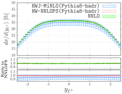
Figure 7: Transverse momentum and rapidity of the positively charged lepton $\ell^{+}$.

We can see that there is a clear agreement between NNLO predictions and NNLOPS results. Other interesting variables are the azimuthal angle between $\ell^{+}$ and the neutrino, $\Delta\phi_{\scriptscriptstyle\ell^{+}\nu}$, and the transverse mass of the $W^{+}$ boson, defined as

$$m_{\scriptscriptstyle T,W}=\sqrt{2p_{t,\nu}\,p_{t,\ell+}(1-\cos(\Delta\phi_{\ell+,\nu}))}\,.$$ (14)

These two variables have characteristic shapes and we show in Fig. 8 that, as expected, our NNLOPS code agrees very well with pure NNLO predictions.

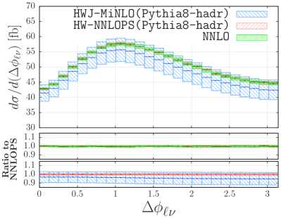
Figure 8: The transverse mass of the $W^{+}$ boson (left) and the azimuthal angle between $\ell^{+}$ and the neutrino (right).

5.3 Jet observables

We present now the study of observables involving final state jets. We will focus on the differences in distributions coming from NNLO, and HVNNLOPS at both parton and hadron level.

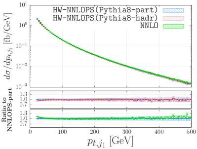
Figure 9: The transverse momentum of the two hardest jets at NNLO (green), HW-NNLOPS before hadronization (blue) and HW-NNLOPS with hadronization (red).

In Fig. 9 we show the transverse momentum of two hardest jets. The distributions are cut at the minimum transverse momentum used for jets, i.e. $20$ GeV, but, from the ratio plot, one can see that the fixed order NNLO calculation starts increasing sharply as it approaches a divergence at low-$p_{t}$. As we identify only jets with $p_{t}>20$ GeV we do not see the Sudakov peak in the HW-NNLOPS simulations, which sits below the cut.

We will first discuss differences between the pure fixed order calculation (green) and the NNLOPS result before hadronization (blue). At large transverse momenta, theoretical uncertainties for the first jet (Fig. 9, left) are of comparable size in all simulations, even if they are slightly smaller in the NNLO calculation. We should also note that, as in the case of $p_{\scriptscriptstyle\mathrm{t,HW}}$, the HVNNLO result is larger than the HVNNLOPS one for large-$p_{t}$ values. This behaviour is a result of using a fixed scale in the former, and a dynamical scale in the latter code.

For the second jet transverse momentum distribution (Fig. 9, right), we note that, as expected, the theoretical uncertainty is larger than in the previous case, as the second jet is described only with LO accuracy. However we note that the scale variation procedure now gives smaller bands for the HVNNLOPS simulation, compared to the NNLO calculation. This is due to the fact Hamilton:2013fea that POWHEG produces additional radiation (the second jet in the case of HWJ-MiNLO) with a procedure that is insensitive to scale variation. The second jet spectrum is multiplied by the NLO cross section kept differential only in the underlying Born variables, i.e. the $\bar{B}$ function. Scale variation affects only the computation of this function (which is NLO accurate), hence as a result the uncertainty due to scale variation for the $p_{\scriptscriptstyle\mathrm{t,j_{2}}}$ spectrum is underestimated with respect to a standard fixed-order computation. We recall that this is a known issue in POWHEG simulations, and was discussed in several previous publications Alioli:2008tz ; Alioli:2010xd . In order to get a more reliable uncertainty band, one can split the real contribution into a singular part (which enters in both the $\bar{B}$ function and the POWHEG Sudakov) and a finite one, corresponding to two resolved emissions. By not including the latter contribution in the $\bar{B}$ function and in the POWHEG Sudakov, the estimation of scale uncertainty would be more similar to what one expects for an observable which is described at LO, as the second-jet high-$p_{T}$ tail.

Next we find it interesting to examine the size of non-perturbative effects. Hadronization has a sizable impact on the shapes of jet distributions: differences up to $7-8$ % can be seen in the $p_{t,j1}$ spectrum at small values, and are still visible at a few percent level till relatively hard jets are required ($p_{\scriptscriptstyle\mathrm{t,j_{1}}}>100$ GeV). For the second jet, hadronization corrections are similar and only slightly more pronounced. Even larger effects can be seen in the rapidity distribution of the two leading jets at large rapidities, as can be seen from Fig. 10. This is not surprising since the large rapidity region is dominated by small transverse momenta.

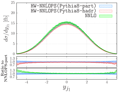
Figure 10: The rapidity of the two hardest jets in NNLO (green), HW-NNLOPS before hadronization (blue) and HW-NNLOPS with hadronization (red).

We have also studied a few dijet observables. In Fig. 11 we present a comparison between the various simulations for the rapidity difference (left) and the invariant mass of the two hardest jets (right).

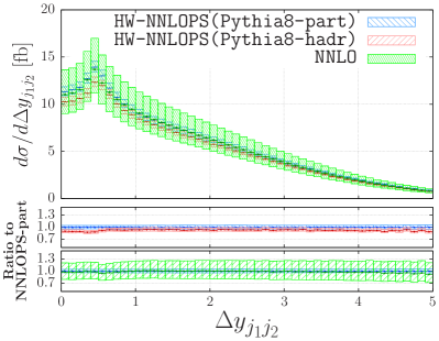
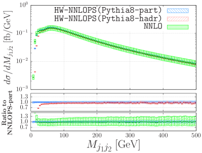
Figure 11: Rapidity difference (left) and invariant mass (right) of two hardest jets in NNLO (green), HW-NNLOPS (blue) and HW-NNLOPS with hadronization (red).

We can see that $\Delta y_{\scriptscriptstyle j_{1},j_{2}}$ displays a peak in the bin just above $\Delta y=0.4$ which is consistent with the jet radius ($R=0.4$) we used for clustering jets. A similar peak is present also in the distribution of the azimuthal angle between the jets $\Delta\phi_{\scriptscriptstyle j_{1},j_{2}}$. We notice that the invariant mass distribution has a peak and a noticeable shoulder (partially washed away after hadronization) at about 55-60 and 20-35 GeV, respectively. Their origin can be understood from the peaks in the $\Delta y_{\scriptscriptstyle j_{1},j_{2}}$ and $\Delta\phi_{\scriptscriptstyle j_{1},j_{2}}$ distributions. In fact the invariant mass can be written as $M_{\scriptscriptstyle j_{1}j_{2}}=2p_{\scriptscriptstyle t,j_{1}}p_{\scriptscriptstyle t,j_{2}}(\cosh\Delta y_{\scriptscriptstyle j_{1},j_{2}}-\cos\Delta\phi_{\scriptscriptstyle j_{1},j_{2}})$. It is easy to roughly estimate the positions of the structures present in the $M_{\scriptscriptstyle j_{1}j_{2}}$ plot: they correspond to when the transverse momenta of the jets are close to the transverse momentum cut, one of the variables ($\Delta y_{j_{1},j_{2}}$ or $\Delta\phi_{j_{1},j_{2}}$) is close to its peak and the other one is integrated over.

Finally, we examine production rates when binned into six regions according to the transverse momentum of the Higgs boson (3 bins corresponding to $0<p_{t,\scriptscriptstyle\textrm{H}}<150$ GeV, $150<p_{t,\scriptscriptstyle\textrm{H}}<250$ GeV, and $250$ GeV$<p_{t,\scriptscriptstyle\textrm{H}}$) and the presence or absence of an additional jet (with jet-veto or with one or more jets). In Fig. 12 we show the six cross-sections, after showering HW-NNLOPS(LHE) events with Pythia8 (HW-NNLOPS) with and without hadronization, and the pure NNLO predictions. We notice that, due to radiation that ends up outside the jet, jets may be softened during parton shower evolution and hence the jet-veto cross-sections are larger at HW-NNLOPS at parton level level compared to pure NNLO level. Differences can reach up to about 15% in the zero-jet bin when the Higgs boson has large transverse momentum. This effect is strengthened once hadronization is applied, since hadronization soften the leading jet spectrum even further. In this case differences up to about 20% can be found compared to pure NNLO predictions. One reason for these sizable differences between NNLO and HW-NNLOPS predictions is that the jet threshold used here is relatively soft ($20$ GeV). In this region the NNLO prediction is starting to diverge and the the leading jet transverse momentum spectrum is particularly sensitive to soft emissions and hadronization effects, as shown in Fig. 9. Furthermore, increasing the value of the jet radius would limit the impact of out-of-jet radiation. Nevertheless, these numbers demonstrate that the merging NNLO calculations to parton showers can be very important when realistic fiducial cuts are applied.

Figure 12: Total cross-section binned according to the transverse momentum of the Higgs boson and the presence of jets. Jets are defined using the anti-$k_{t}$ algorithm with $R=0.4$, $p_{t,j}>20$ GeV and $|y_{j}|<4.5$. Results are shown at various levels of the simulation, see text for more details.

6 Conclusion

In this paper we have used the MiNLO-based merging method to obtain the first NNLO accurate predictions for HW production consistently matched to a parton shower, including the decay of the W boson to leptons. The method requires a multi-differential reweighting of the weight of HWJ-MiNLO events to the NNLO accurate Born distributions. We have used that the $K-$factor, within our statistical accuracy, is independent of the mass of the dilepton system over the whole phase space, hence we have performed the reweighting in the three Born variables $\{y_{\scriptscriptstyle\textrm{HW}}{},\Delta y_{\scriptscriptstyle\textrm{HW}}{},p_{t,\scriptscriptstyle\textrm{H}}{}\}$ and in the two Collins-Soper angles that describe the decay of the $W$ boson. For the latter variables, we have exploited the fact that the kinematic dependence can be parametrized in terms of spherical harmonics of degree up to two.

For our phenomenological results, we have considered a setup suggested recently in the context of the Higgs cross section working group. We find that including NNLO corrections in the MiNLO simulation reduces scale variation uncertainties from about 10% to about 1-2%. Compared to a pure NNLO calculation, while the perturbative accuracy is the same, our tool allows one to perform fully realistic simulations, including the study of non-perturbative effects and multi-parton interactions.

By construction, for leptonic observables we find that the NNLO and NNLOPS simulations agree when no cut on additional radiation is imposed. However, we find sizable differences between the two simulations when realistic cuts are imposed. This is particularly the case in the region where the Higgs boson is boosted and a jet-veto condition is imposed. In this case differences amount to about 15% at the 13 TeV LHC. This large effect is due to a migration of events that, before the parton shower, have a soft jet (whose transverse momentum is just above the veto scale) from the one-jet to the zero-jet category. In fact, with our setup, the main effect of the parton shower is to soften the leading jet, therefore increasing the fraction of events that fall into the zero-jet category. Different jet-thresholds and jet-radii leads to quite different conclusions. Still, these differences are in general outside the scale-variation uncertainties of the NNLO calculation, hence the NNLOPS accurate prediction becomes important to provide a more realistic uncertainty estimate. The HVNNLOPS generator we have developed will allow to simulate these features in a fully-exclusive way, retaining at the same time all the virtues of an NNLO computation for fully inclusive observables, as well as resummation effects, thanks to the interplay among POWHEG, MiNLO and parton showering.

Appendix A Pure NNLO Uncertainties

This section we compare the 49 scale method we used, as detailed in Sec. 3.3, to the 21 scale method used for HNNLOPS Hamilton:2013fea and DYNNLOPS Karlberg:2014qua . To do this we repeated our analysis using the 21 scale uncertainty method, with $(K_{\scriptscriptstyle\mathrm{R}},K_{\scriptscriptstyle\mathrm{F}})=(0.5,0.5),(1,1),(2,2)$ for the fixed order NNLO results. We find that in general both methods result in uncertainty bands they are very similar, with the 49 scale uncertainty band being only 1-2 permille larger in some bins.

There are however few cases where having only 21 scales results in noticeably smaller uncertainty bands than 49 scales. To quantify better the differences between the two uncertainties from the two methods, we show in Fig. 13 four observables for which we found the largest differences in uncertainties bands.

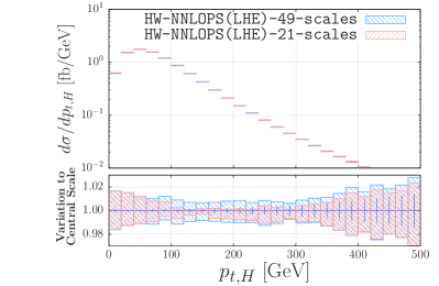
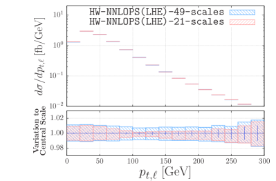
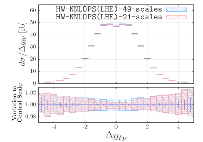
Figure 13: Comparison of the uncertainty from the envelope of 49 scale variations (blue) vs 21 scale variations (green) for $p_{t,\scriptscriptstyle\textrm{H}}$ (upper left), $p_{t,\scriptscriptstyle\ell}$ (upper right), for $m_{\scriptscriptstyle HW}$ (lower left), and for $\Delta y_{\ell\nu}$. Statistical error of the central scale result shown for reference.

References

- (1) G. Aad et al. [ATLAS Collaboration], Phys. Lett. B 716, 1 (2012) [arXiv:1207.7214 [hep-ex]]
- (2) S. Chatrchyan et al. [CMS Collaboration], Phys. Lett. B 716, 30 (2012) [arXiv:1207.7235 [hep-ex]]
- (3) G. Aad et al. [ATLAS Collaboration], JHEP 1501, 069 (2015) [arXiv:1409.6212 [hep-ex]]
- (4) S. Chatrchyan et al. [CMS Collaboration], Phys. Rev. D 89, no. 1, 012003 (2014) [arXiv:1310.3687 [hep-ex]]
- (5) The ATLAS collaboration, ATLAS-CONF-2013-075.
- (6) The CMS Collaboration, CMS-PAS-HIG-13-009.
- (7) The CMS Collaboration, CMS-PAS-HIG-12-053.
- (8) S. Chatrchyan et al. [CMS Collaboration], Eur. Phys. J. C 74, 2980 (2014) [arXiv:1404.1344 [hep-ex]]
- (9) J. M. Butterworth, A. R. Davison, M. Rubin and G. P. Salam, Phys. Rev. Lett. 100, 242001 (2008) [arXiv:0802.2470 [hep-ph]]
- (10) O. Brein, A. Djouadi and R. Harlander, Phys. Lett. B 579, 149 (2004) [hep-ph/0307206]
- (11) G. Ferrera, M. Grazzini and F. Tramontano, Phys. Rev. Lett. 107, 152003 (2011) [arXiv:1107.1164 [hep-ph]]
- (12) G. Ferrera, M. Grazzini and F. Tramontano, Phys. Lett. B 740, 51 (2015) [arXiv:1407.4747 [hep-ph]]
- (13) O. Brein, R. Harlander, M. Wiesemann and T. Zirke, Eur. Phys. J. C 72, 1868 (2012) [arXiv:1111.0761 [hep-ph]]
- (14) G. Ferrera, M. Grazzini and F. Tramontano, JHEP 1404, 039 (2014) [arXiv:1312.1669 [hep-ph]]
- (15) M. L. Ciccolini, S. Dittmaier and M. Kramer, Phys. Rev. D 68, 073003 (2003) [hep-ph/0306234]
- (16) A. Denner, S. Dittmaier, S. Kallweit and A. Muck, JHEP 1203, 075 (2012) [arXiv:1112.5142 [hep-ph]]
- (17) A. Denner, S. Dittmaier, S. Kallweit and A. Muck, Comput. Phys. Commun. 195, 161 (2015) [arXiv:1412.5390 [hep-ph]]
- (18) J. M. Campbell, R. K. Ellis and C. Williams, [arXiv:1601.00658 [hep-ph]]
- (19) A. Banfi, P. F. Monni, G. P. Salam and G. Zanderighi, Phys. Rev. Lett. 109, 202001 (2012) [arXiv:1206.4998 [hep-ph]]
- (20) T. Becher, R. Frederix, M. Neubert and L. Rothen, Eur. Phys. J. C 75, no. 4, 154 (2015) [arXiv:1412.8408 [hep-ph]]
- (21) S. Frixione and B. R. Webber, JHEP 0206, 029 (2002) [hep-ph/0204244]
- (22) P. Nason, JHEP 0411, 040 (2004) [hep-ph/0409146]
- (23) S. Frixione and B. R. Webber [hep-ph/0506182]
- (24) G. Luisoni, P. Nason, C. Oleari and F. Tramontano, JHEP 1310, 083 (2013) [arXiv:1306.2542 [hep-ph]]
- (25) D. Goncalves, F. Krauss, S. Kuttimalai and P. Maierhöfer, Phys. Rev. D 92 (2015) 7, 073006 [arXiv:1509.01597 [hep-ph]]
- (26) K. Hamilton, P. Nason and G. Zanderighi, JHEP 1210, 155 (2012) [arXiv:1206.3572 [hep-ph]]
- (27) K. Hamilton, P. Nason, C. Oleari and G. Zanderighi, JHEP 1305, 082 (2013) [arXiv:1212.4504 [hep-ph]]
- (28) K. Hamilton, P. Nason, E. Re and G. Zanderighi, JHEP 1310, 222 (2013) [arXiv:1309.0017 [hep-ph]]
- (29) A. Karlberg, E. Re and G. Zanderighi, JHEP 1409, 134 (2014) [arXiv:1407.2940 [hep-ph]]
- (30) R. Frederix and K. Hamilton, [arXiv:1512.02663 [hep-ph]]
- (31) J. C. Collins and D. E. Soper, Phys. Rev. D 16 (1977) 2219.
- (32) S. Catani, Y. L. Dokshitzer, M. H. Seymour and B. R. Webber, Nucl. Phys. B 406 (1993) 187.
- (33) S. D. Ellis and D. E. Soper, Phys. Rev. D 48 (1993) 3160 [hep-ph/9305266]
- (34) G. Ferrera, M. Grazzini, F. Tramontano, private communication.
- (35) S. Alioli, P. Nason, C. Oleari and E. Re, JHEP 1006 (2010) 043 [arXiv:1002.2581 [hep-ph]]
- (36) L. A. Harland-Lang, A. D. Martin, P. Motylinski and R. S. Thorne, Eur. Phys. J. C 75 (2015) 5, 204 [arXiv:1412.3989 [hep-ph]]
- (37) M. Cacciari, G. P. Salam and G. Soyez, JHEP 0804 (2008) 063 [arXiv:0802.1189 [hep-ph]]
- (38) M. Cacciari and G. P. Salam, Phys. Lett. B 641 (2006) 57 [hep-ph/0512210]
- (39) M. Cacciari, G. P. Salam and G. Soyez, Eur. Phys. J. C 72 (2012) 1896 [arXiv:1111.6097 [hep-ph]]
- (40) T. Sjostrand, S. Mrenna and P. Z. Skands, Comput. Phys. Commun. 178 (2008) 852 [arXiv:0710.3820 [hep-ph]]
- (41) P. Skands, S. Carrazza and J. Rojo, Eur. Phys. J. C 74 (2014) 8, 3024 [arXiv:1404.5630 [hep-ph]]
- (42) P. Nason and C. Oleari, [arXiv:1303.3922 [hep-ph]]
- (43) A. Banfi, G. P. Salam and G. Zanderighi, JHEP 1206 (2012) 159 [arXiv:1203.5773 [hep-ph]]
- (44) S. Alioli, P. Nason, C. Oleari and E. Re, JHEP 0904 (2009) 002 [arXiv:0812.0578 [hep-ph]]