Signatures of Gravitational Instability in Resolved Images of Protostellar Disks

Abstract

Protostellar (class 0/I) disks, having masses comparable to those of their nascent host stars, and fed continuously from their natal infalling envelopes, are prone to gravitational instability (GI). Motivated by advances in near-infrared (NIR) adaptive optics imaging and mm-wave interferometry, we explore the observational signatures of GI in disks, using hydrodynamical and Monte Carlo radiative transfer simulations to synthesize NIR scattered light images and mm dust continuum maps. Spiral arms induced by GI, located at disk radii of hundreds of AUs, are local overdensities and have their photospheres displaced to higher altitudes above the disk midplane; arms therefore scatter more NIR light from their central stars than inter-arm regions, and are detectable at distances up to 1 kpc by Gemini/GPI, VLT/SPHERE, and Subaru/HiCIAO/SCExAO. By contrast, collapsed clumps formed by disk fragmentation have such strong local gravitational fields that their scattering photospheres are at lower altitudes; such fragments appear fainter than their surroundings in NIR scattered light. Spiral arms and streamers recently imaged in four FU Ori systems at NIR wavelengths resemble GI-induced structures and support the interpretation that FUors are gravitationally unstable protostellar disks. At mm wavelengths, both spirals and clumps appear brighter in thermal emission than the ambient disk and can be detected by ALMA at distances up to 0.4 kpc with one-hour integration times at $\sim$0.1$\arcsec$ resolution. Collapsed fragments having masses $\gtrsim 1M_{\rm J}$ can be detected by ALMA within $\sim$10 minutes.

1 Introduction

Both stellar and substellar companions can be spawned within gaseous accretion disks around newly born stars. At early times, the mass of the disk can be significant compared with the still-forming central star, and the mass infall rate from the disk’s natal envelope can be larger than the accretion rate through the disk. Such young and unsteady disks experience gravitational instability (GI) if they satisfy the $Q$ criterion (Goldreich & Lynden-Bell, 1965):

$$Q=\frac{c_{\rm s}\Omega}{\pi{\rm G}\Sigma}\lesssim{\rm unity},$$ (1)

where $c_{\rm s}$, $\Omega$, and $\Sigma$ are the disk’s sound speed, orbital frequency, and surface density. Gravitationally unstable disks have been simulated extensively (e.g., Vorobyov & Basu, 2005, 2006, 2010b; Boley et al., 2010; Machida et al., 2011b; Tsukamoto et al., 2013; Zhu et al., 2012a). The disks may also fragment if they cool sufficiently fast (e.g., Gammie, 2001; Rice et al., 2003; Rafikov, 2009; Shi & Chiang, 2014):

$$\beta=t_{\rm cool}\Omega\lesssim{\rm a\ few},$$ (2)

where $t_{\rm cool}$ is the cooling timescale. Disk fragmentation can result in bound self-gravitating objects, and is thought to be a channel for the formation of giant planets, brown dwarfs, or stars.

We can enumerate a number of observational consequences of GI in protostellar/protoplanetary disks:

1. GI excites large-scale spiral arms, which may be visible in resolved observations at near-infrared (NIR; e.g., Dong et al., 2015a; Pohl et al., 2015) and mm wavelengths (e.g., Cossins et al., 2010; Vorobyov et al., 2013; Dipierro et al., 2014).

2. At large orbital distances from the star, disk fragmentation may form bound objects such as giant planets, brown dwarfs, or stellar mass companions (e.g., Boss, 1997; Rice et al., 2005; Rafikov, 2005; Stamatellos & Whitworth, 2009; Kratter et al., 2010; Meru & Bate, 2011; Machida et al., 2011b; Vorobyov & Basu, 2010a; Vorobyov, 2013). These objects, or their circumsecondary disks (e.g., Kraus et al., 2015; Caceres et al., 2015), may be detectable by adaptive optics (AO) imaging (e.g., Kraus & Ireland, 2012; Bowler et al., 2013; Kuzuhara et al., 2013).

3. GI (possibly in combination with other disk instabilities such as the magnetorotational instability) can trigger outbursts (e.g., Vorobyov & Basu, 2005, 2006, 2010b; Zhu et al., 2009; Machida et al., 2011b; Bae et al., 2014; Vorobyov & Basu, 2015), detectable as abrupt and possibly repetitive surges in the accretion luminosity. The accretion outbursts in FU Orionis objects (FUor; Hartmann et al., 1998; Audard et al., 2014) and in some EX Orionis objects (EXor; Herbig, 2008) have been suggested to be triggered by GI.

4. The gas kinematics in self-gravitating disks deviates from Keplerian. These deviations may be detectable in molecular line observations (e.g., Rosenfeld et al., 2014).

Historically, program 1 — resolved imaging — has been difficult to pursue. Young disks are often embedded in and highly extincted by gaseous envelopes at optical to NIR wavelengths. FUors and EXors are rare and typically found in distant clusters of young stellar objects (e.g., Orion at $\sim$400 pc). To resolve GI-induced spiral arms and fragments at these distances demands 0.1$\arcsec$ or better angular resolution, and sub-arcsec inner working angles. Observations of possibly GI-unstable class 0/I objects (Andre & Montmerle 1994) have so far been mostly indirect/photometric.

The situation, however, has been recently evolving, thanks to technological advances in both NIR direct imaging and mm-wave interferometry. At NIR wavelengths, a fleet of new instruments equipped with extreme adaptive optics and polarimetric differential imaging (PDI; e.g., Perrin et al., 2004; Hinkley et al., 2009) has been deployed, including VLT/SPHERE (Beuzit et al., 2008), Gemini/GPI (Macintosh et al., 2008), and Subaru/HiCIAO/SCExAO (Jovanovic et al., 2015). At mm wavelengths, the new interferometers ALMA and JVLA are probing young stellar objects with unprecedentedly high sensitivity and resolution. Liu et al. (2016b) directly imaged four FUors using Subaru/HiCIAO with sub-0.1$\arcsec$ angular resolution: FU Ori, V1735 Cyg, V1057 Cyg, and Z CMa (see also the VLT/NaCo observation of Z CMa by Canovas et al. 2015). Polarization vector analysis confirmed that these objects contain disks. Large-scale asymmetric structures such as spirals and streamers, possibly produced by GI, were discerned at stellocentric distances of hundreds of AU. With its sub-0.05$\arcsec$ resolution, ALMA resolved the class 0/I disk HL Tau (ALMA Partnership et al., 2015), which has an estimated mass of $\gtrsim 0.1M_{\odot}$ ($\gtrsim 0.2$ times the mass of its central star $M_{\star}$; Greaves et al. 2008; Kwon et al. 2011) and whose self-gravity may be significant (Takahashi & Inutsuka, 2014; Jin et al., 2016).

Looking ahead, we anticipate a great many images of class 0/I disks to become available at high angular resolution in the next decade. These new data will help to answer key questions in disk evolution and planet formation: How long is the GI-unstable phase? Do companions form through disk fragmentation? What are the nature of FUor and EXor outbursts? Motivated by these upcoming observations, in this paper we synthesize images of gravitationally unstable protostellar/protoplanetary disks at early times $\lesssim 0.5$ Myr, when infall from the envelope is still occurring. We employ the Vorobyov & Basu (2015) hydrodynamics code to simulate the formation and evolution of a disk-star system directly from the collapse of a rotating, initially starless cloud core. The results of the hydro code are fed into the Whitney et al. (2013) Monte Carlo radiative transfer (MCRT) code to produce synthetic images of the disk. We focus on direct imaging of the NIR polarized intensity (PI), and on interferometric maps of the mm-wave dust thermal emission. The goal is to make predictions for future resolved observations, and in particular to answer the question of whether GI-induced spiral arms and fragments are detectable in NIR imaging observations using Gemini/GPI, VLT/SPHERE, and Subaru/HiCIAO/SCExAO, and in mm dust continuum observations using ALMA.

Some groundwork on synthesizing images has been laid. Vorobyov et al. (2013) carried out semianalytic calculations to create mock ALMA observations of GI-unstable disks. They did not examine the properties of the disk in scattered light, nor did they consider non-face-on viewing angles. These limitations are removed in our work. Stamatellos et al. (2011) simulated ALMA observations of GI-unstable disks produced by their smoothed particle hydrodynamics code. We relax their assumptions that dust has a constant temperature and is optically thin. The appearance of GI-induced spiral arms and clumps has been studied by Cossins et al. (2010), Douglas et al. (2013) and Mayer et al. (2016) at mm wavelengths and by Dong et al. (2015a) at NIR wavelengths; these works focused on isolated systems (i.e., those without infalling envelopes) and on small scales ($\sim$100 AU); moreover, the systems were only evolved for a few tens of thousand years or less.

The structure of our paper is as follows. We introduce our hydrodynamics simulation in Section 2.1 and our MCRT simulations in Section 2.2. The results of the hydro simulation are presented in Section 3.1, and synthetic images are shown in NIR scattered light in Section 3.2 and in the mm-wave thermal continuum in Section 3.3. In Section 4.1 we discuss the limitations of our models, and in Section 4.2 we review the near-term prospects for observing GI-unstable young disks. Section 5 summarizes.

2 Simulations

We carry out a 2+1D hydrodynamics simulation to model the formation and evolution of a disk-star system directly from the collapse of an initially starless, rotating molecular cloud core. The hydro code (Section 2.1) is adopted largely from Vorobyov & Basu (2015) with a few improvements as described below. The gas surface density is calculated from the hydro simulation at 6 epochs. For insertion into the Whitney et al. (2013) MCRT code (Section 2.2), the 2D surface density from the hydro model is “puffed up” vertically into a 3D density field by assuming hydrostatic equilibrium, using an approximate temperature and vertical scale height inferred from the hydro model. The MCRT code produces both scattered light and thermal emission maps; the latter are computed from dust temperatures calculated in detail from the MCRT model.

2.1 Hydrodynamical Simulation

We start our numerical simulation from the gravitational collapse of a starless cloud core, continue into the embedded phase of star formation — during which a star, disk, and envelope are formed — and terminate our simulations at $t\sim 0.5$ Myr when the envelope dissipates after accreting onto the star+disk system. Long integration times are made possible by the use of the thin-disk (2D) approximation. This approximation enables us to follow the evolution of the disk for many orbital periods and its justification is discussed in Vorobyov & Basu (2010b). Once formed, the protostellar disk occupies the inner part of the numerical polar grid (usually, several hundreds of AU), while the contracting envelope occupies the rest of the grid (which may extend to several thousands of AU).

To avoid time steps that are too short, we introduce a “sink cell” at $r_{\rm sc}=10.0$ AU and impose a free outflow boundary condition so that matter is allowed to flow out of the computational domain but is prevented from flowing in. During the early stages of core collapse, we monitor the gas surface density in the sink cell; when its value exceeds a critical value for the transition from isothermal to adiabatic evolution, we introduce a first hydrostatic core (FHSC) with a size equal to that of the sink cell. The parameters of the FHSC are calculated assuming a simple polytropic sphere model with index $n=2.5$ ($\gamma=7/5$). When the temperature in the center of the FHSC exceeds 2000 K (triggering the dissociation of molecular hydrogen) or its mass exceeds 0.05 $M_{\odot}$ (as suggested by radiation transfer calculations of Masunaga & Inutsuka 2000), we assume that the second collapse ensues and a central protostar forms. In the subsequent evolution, 90% of the gas that crosses the inner boundary is assumed to land on the protostar. The other 10% of the accreted gas is assumed to be carried away by protostellar jets. The FHSC stage is usually short (tens of thousands of years) compared to the protostellar stage (several hundred thousand years).

The equations of mass, momentum, and energy transport in the thin-disk limit are

$$\frac{{\partial\Sigma}}{{\partial t}}=-\nabla_{p}\cdot\left(\Sigma\mbox{\boldmath$v$}_{p}\right),$$ (3)

$$\frac{\partial}{\partial t}\left(\Sigma\mbox{\boldmath$v$}_{p}\right)+\left[\nabla\cdot\left(\Sigma\mbox{\boldmath$v$}_{p}\otimes\mbox{\boldmath$v$}_{p}\right)\right]_{p}=-\nabla_{p}{\cal P}+\Sigma\,\mbox{\boldmath$g$}_{p}+(\nabla\cdot\mathbf{\Pi})_{p}$$ (4)

$$\frac{\partial e}{\partial t}+\nabla_{p}\cdot\left(e\mbox{\boldmath$v$}_{p}\right)=-{\cal P}(\nabla_{p}\cdot\mbox{\boldmath$v$}_{p})-\Lambda+\Gamma+\left(\nabla\mbox{\boldmath$v$}\right)_{pp^{\prime}}:\Pi_{pp^{\prime}},$$ (5)

where subscripts $p$ and $p^{\prime}$ refers to the planar components $(r,\phi)$ in polar coordinates, $\Sigma$ is the mass surface density, $e$ is the internal energy per surface area, ${\cal P}$ is the vertically integrated gas pressure calculated via the ideal equation of state as ${\cal P}=(\gamma-1)e$, $\mbox{\boldmath$v$}_{p}=v_{r}\hat{\mbox{\boldmath$r$}}+v_{\phi}\hat{\mbox{\boldmath$\phi$}}$ is the velocity in the disk plane, and $\nabla_{p}=\hat{\mbox{\boldmath$r$}}\partial/\partial r+\hat{\mbox{\boldmath$\phi$}}r^{-1}\partial/\partial\phi$. Turbulent viscosity is taken into account via the viscous stress tensor $\mathbf{\Pi}$, the expression for which is provided in Vorobyov & Basu (2010b). We parameterize the magnitude of kinematic viscosity $\nu$ using the $\alpha$-prescription with a spatially and temporally uniform $\alpha=0.01$. The ratio of specific heats is calculated by assuming that $\gamma=5/3$ below 100 K and $\gamma=7/5$ above 100 K. We apply a smooth transition at the critical temperature to avoid sharp changes in the values of $\gamma$. This form of $\gamma$ takes into account the fact that the rotational and vibrational degrees of freedom of molecular hydrogen are excited only above 100 K.

The gravitational acceleration in the disk plane, $\mbox{\boldmath$g$}_{p}=g_{r}\hat{\mbox{\boldmath$r$}}+g_{\phi}\hat{\mbox{\boldmath$\phi$}}$, takes into account the self-gravity of the disk and the gravity of the central protostar when formed. The former component is found by solving for the Poisson integral

$$\Phi(r,\phi) = -G\int_{r_{\rm sc}}^{r_{\rm out}}r^{\prime}dr^{\prime}$$ (6)

$$\times\int_{0}^{2\pi}\frac{\Sigma(r^{\prime},\phi^{\prime})d\phi^{\prime}}{\sqrt{{r^{\prime}}^{2}+r^{2}-2rr^{\prime}\cos(\phi^{\prime}-\phi)}}\,,$$

where $r_{\rm out}$ is the radial position of the computational outer boundary (equivalently, the initial radius of the cloud core). This integral is calculated using a FFT technique which applies the 2D Fourier convolution theorem for polar coordinates (see Binney & Tremaine, 1987, Sect. 2.8).

An approximate expression for the radially and azimuthally varying vertical scale height $h$ is determined in each computational cell via the equation of local vertical pressure balance (Vorobyov & Basu, 2009):

$$\rho\,\tilde{c}_{s}^{2}=2\int_{0}^{h}\rho\left(g_{z,\rm gas}+g_{z,\rm st}\right)dz,$$ (7)

where $\rho$ is the gas volume density, $g_{z,\rm gas}$ and $g_{z,\rm st}$ are the vertical gravitational accelerations due to disk self-gravity and the gravitational pull of the central star, respectively, and $\tilde{c}^{2}_{s}=\partial{\cal P}/\partial\Sigma$ is the effective sound speed of the non-isothermal gas. Assuming that $\rho$ is a slowly varying function of vertical distance $z$ between $z=0$ (midplane) and $z=h$ — i.e., $\Sigma=2\,h\,\rho$ — and using Gauss’s theorem, one can show that

$$\int_{0}^{h}\rho\,g_{z,\rm gas}\,dz = \frac{\pi}{4}G\Sigma^{2}\>,$$ (8)

$$\int_{0}^{h}\rho\,g_{z,\rm st}\,dz = \frac{GM_{\ast}\rho}{r}\left\{1-\left[1+\left({\Sigma\over 2\rho r}\right)\right]^{-1/2}\right\},$$ (9)

where $M_{\ast}$ is the mass of the central star. Substituting equations (8) and (9) back into equation (7), we obtain

$$\rho\,\tilde{c}_{s}^{2}={\pi\over 2}G\Sigma^{2}+{2GM_{\ast}\rho\over r}\left\{1-\left[1+\left({\Sigma\over 2\rho r}\right)\right]^{-1/2}\right\}.$$ (10)

This can be solved for $\rho$ given the model’s known $\tilde{c}_{s}^{2}$, $\Sigma$, and $M_{\ast}$, using Newton-Raphson iteration. The vertical scale height is finally derived as

$$h=\frac{\Sigma}{2\rho}.$$ (11)

This height is used to calculate the stellar flux incident upon the disk surface, as per equation (15) below, and to enable a connection to our 3D MCRT code, as described in Section 2.2.

The radiative cooling per surface area in equation (5) is determined using the diffusion approximation for vertical radiation transport in a one-zone model (see the Appendix for details)

$$\Lambda=\frac{4\tau_{\rm P}\sigma T_{\rm hydro}^{4}}{1+2\tau_{\rm P}+{3\over 2}\tau_{\rm R}\tau_{\rm P}},$$ (12)

where $\sigma$ is the Stefan-Boltzmann constant, $T_{\rm hydro}={\cal P}\mu/{\cal R}\Sigma$ is the temperature (“hydro” to distinguish this temperature from the temperature calculated from the MCRT code later), $\mu=2.33$ the mean molecular weight, $\cal R$ the universal gas constant, $\tau_{\rm R}=\kappa_{\rm R}\Sigma_{1/2}$ and $\tau_{\rm P}=\kappa_{\rm P}\Sigma_{1/2}$ the Rosseland and Planck optical depths to the disk midplane, and $\Sigma_{1/2}=\Sigma/2$ the gas surface density from the disk surface to the midplane. The Planck and Rosseland mean opacities are calculated from the opacity tables by Semenov et al. (2003). The heating function per surface area of the disk is expressed as

$$\Gamma=\frac{4\tau_{\rm P}\sigma T_{\rm irr}^{4}}{1+2\tau_{\rm P}+{3\over 2}\tau_{\rm R}\tau_{\rm P}},$$ (13)

where $T_{\rm irr}$ is the irradiation temperature at the disk surface determined by the stellar and background blackbody radiation fields as

$$T_{\rm irr}^{4}=T_{\rm bg}^{4}+\frac{F_{\rm irr}(r)}{\sigma},$$ (14)

where $T_{\rm bg}$ is the uniform background temperature (set to the initial temperature of the natal cloud core) and $F_{\rm irr}(r)$ is the radiation flux (energy per unit time per unit surface area) absorbed by the disk surface from the central star. The latter quantity is calculated as

$$F_{\rm irr}(r)=\frac{L_{\ast}}{4\pi r^{2}}\cos{\gamma_{\rm irr}},$$ (15)

where $\gamma_{\rm irr}$ is the incidence angle of radiation arriving at the disk surface (with respect to the normal). The incidence angle is calculated using the disk vertical scale height $h$, as described in Vorobyov & Basu (2010b); disk self-shielding is not taken into account in the present study.

The stellar luminosity $L_{\ast}$ is the sum of the accretion luminosity $L_{\rm\ast,accr}=(1-\epsilon)GM_{\ast}\dot{M}/2R_{\ast}$ arising from the gravitational energy of accreted gas and the photospheric luminosity $L_{\rm\ast,ph}$ due to gravitational contraction and deuterium burning in the stellar interior. The stellar mass $M_{\ast}$ and accretion rate onto the star $\dot{M}$ are determined from the amount of gas passing into the sink cell. The properties of the forming protostar ($L_{\rm\ast,ph}$ and radius $R_{\ast}$) are calculated using the Lyon stellar evolution code described in Baraffe & Chabrier (2010). As in Baraffe et al. (2012), we assume that a fraction $\epsilon$ of the accretion energy $GM_{\ast}{\dot{M}}/(2{R_{\ast}})$ is absorbed by the protostar, while the remaining fraction $(1-\epsilon$) is radiated away and contributes to the accretion luminosity of the star $L_{\rm\ast,accr}$. Despite many efforts, the exact value of $\epsilon$ in low-mass star formation is not known. In the present calculations, we adopt a so-called “hybrid” scheme (for details, see Baraffe et al., 2012) with $\epsilon=0$ when accretion rates remain smaller than a critical value $\dot{M}_{\rm cr}=10^{-5}~{}M_{\odot}$ yr^-1, and $\epsilon=0.2$ when $\dot{M}>\dot{M}_{\rm cr}$. The stellar evolution code is coupled with the main hydrodynamical code in real time. Because of the heavy computational load, the stellar evolution code updates the properties of the protostar only every 20 yr, while the hydrodynamical time step may be as short as a few months.

Equations (3)–(5) are solved in polar coordinates on a numerical grid with $512\times 512$ grid zones. The radial grid zones are logarithmically spaced, while the grid spacing in the azimuthal direction is uniform. The details of the solution procedure are given in Vorobyov & Basu (2010b). For initial conditions, we considered a gravitationally unstable pre-stellar core with the following radial profiles of column density $\Sigma$ and angular velocity $\Omega$:

$$\Sigma = {r_{0}\Sigma_{0}\over\sqrt{r^{2}+r_{0}^{2}}}\>,$$ (16)

$$\Omega = 2\Omega_{0}\left({r_{0}\over r}\right)^{2}\left[\sqrt{1+\left({r\over r_{0}}\right)^{2}}-1\right],$$ (17)

where $\Sigma_{0}=5.2\times 10^{-2}$ g cm^-2 and $\Omega_{0}=1.25$ km s^-1 pc^-1 are the gas surface density and angular velocity at the center of the core. These profiles have a small near-uniform central region of size $r_{0}=2400$ AU which transitions to an $r^{-1}$ profile; they are representative of a wide class of observations and theoretical models (Basu, 1997; Andre et al., 1993; Dapp & Basu, 2009). The initial radius of the core is 0.07 pc and its initial temperature is uniform at 10 K. The total mass of the core is 1.08 $M_{\odot}$.

2.2 Monte Carlo Radiative Transfer Simulations

The MCRT simulations largely follow the procedures in Dong et al. (2015b), and are summarized below. We construct a 3D grid in the radial ($r$), azimuthal ($\phi$), and polar ($\theta$) directions. The grid covers from the dust sublimation radius $r_{\rm sub}$ to an outer radius $r_{\rm out}=1000$ AU, $0-2\pi$ in $\phi$, and $0-\pi$ in $\theta$ ($\theta=\pi/2$ is the disk midplane), and has $419\times 512\times 200$ cells in $r\times\phi\times\theta$. At $r\geq r_{\rm in}$ the $r\times\phi$ grid is identical to the polar grid in the hydro model, while from $r_{\rm sub}\leq r<r_{\rm in}$ (a region not covered by the hydro model) the grid is logarithmic in $r$. The sublimation radius $r_{\rm sub}$ is determined for each epoch of the hydro model as where the dust temperature reaches 1600 K ($r_{\rm sub}\sim 0.1$ AU). The grid spacing $\delta\theta$ is linearly proportional to $\theta$ to better resolve the disk midplane. At $1000\geq r({\rm AU})\geq 20$, $\Sigma_{\rm gas}$ is set by the hydro model; at $20\,{\rm AU}\geq r\geq r_{\rm sub}$, $\Sigma_{\rm gas}$ follows a $1/r$ radial profile. We note that the envelope at $r>1000$ AU in the hydro simulation is not included in the MCRT calculations; this omission will be discussed in Section 4.2. To construct 3D disk models from 2D hydro $\Sigma_{\rm gas}$ maps, we assume hydrostatic equilibrium in the vertical direction $z$, and puff up the 2D disk according to a Gaussian profile,

$$\rho_{\rm gas}(z)=\frac{\Sigma_{\rm gas}}{h\sqrt{2\pi}}e^{-z^{2}/2h^{2}},$$ (18)

where $\rho_{\rm gas}$ is the gas volume density and the scale height $h$ is computed from the hydro simulation (Equation 11). This treatment is necessary as 2D hydro simulations are needed to follow the evolution of the system for hundreds of thousands of years, while 3D disk structures are required in the radiative transfer post processing. Millimeter fluxes from our models are not affected by this treatment. At NIR wavelengths, contrasts of disk features may be weakened (Zhu et al., 2015), which enhances our conclusion that GI-induced spiral arms are visible (see below). The central star in MCRT simulations has the same temperature, mass, and luminosity (photospheric+accretion) as determined in the hydro simulation at each epoch (Table LABEL:tab:models). MCRT simulations have only one illumination source (the central star), i.e., the fragments are not self-luminous. All simulations are run with at least 2 billion photon packets.

Millimeter observations have shown evidence of grain growth in class 0/I objects. For example, the $\sim$1 Myr old HL Tau disk is very bright at mm wavelengths, indicating the presence of large grains (ALMA Partnership et al., 2015). Also, Miotello et al. (2014) and Chiang et al. (2012) found low values of the mm spectral index in class I objects. To take grain growth into account, we include two populations of dust grains in the MCRT simulations: small and big grains. Small grains are standard interstellar medium (ISM) grains (Kim et al., 1994) made of silicate, graphite, and amorphous carbon. Their size distribution obeys a power law in the size range of $0.02\lesssim s\lesssim 0.25$ $\micron$, followed by an exponential cut off at larger sizes. Big grains have identical composition, but have grown to a maximum size of 1 mm with a power law size distribution $dn(s)/ds\propto s^{-3}$. The optical properties of both populations can be found in Figure 2 of Dong et al. (2012). The opacity of the big grains is 13 cm² g^-1 at 1.3 mm (dust only, not dust+gas). The scattering phase function of the small grains is approximated using the Henyey & Greenstein (1941) function, and a Rayleigh-like phase function is assumed for the linear polarization (White, 1979).

Dust grains dominate the opacity in disks. Specifically, NIR scattered light arises from the disk surface, and mainly probes the distribution of small grains (both their surface density and vertical distribution). Mm continuum emission is sensitive to the surface density distribution of big grains. To convert $\rho_{\rm gas}$ into $\rho_{\rm grains}$, we assume a total dust-to-gas mass density ratio of 1:100 and a small-to-big dust mass density ratio of 1:9. We assign $\rho_{\rm small\ grains}=10^{-3}\rho_{\rm gas}$ (small grains are well-mixed with gas). For the big grains, we take $\Sigma_{\rm big\ grains}=9\times 10^{-3}\Sigma_{\rm gas}$ and distribute them vertically according to a Gaussian with scale height $h_{\rm big\ grains}=0.5h$ to mimic vertical settling. We note that the specific ratio of $h_{\rm big\ grains}/h$ is not important as long as it is less than 1; the NIR scattered light is more sensitive to the small grains, and the mm continuum emission is not sensitive to the vertical distribution of the big grains.

Full resolution synthesized PI images at $\lambda=1.6\,\micron$ ($H$-band) and mm continuum maps at 1.3 mm (230 GHz; ALMA band 6) and 0.87 mm (345 GHz; ALMA band 7) are produced from the MCRT simulations. Full resolution $H$-band images are then convolved by a Gaussian PSF with a full width half maximum (FWHM) of 0.04$\arcsec$, to simulate the diffraction limited angular resolution of Subaru, VLT, and Gemini. Full resolution mm images are transformed to simulated ALMA observations using the simobserve and simanalyze tools under Common Astronomy Software Applications (CASA). A full array of 50 12-meter antennas is used. Throughout the paper, we use a blue-hot color scheme at $H$-band and a red-hot color scheme for ALMA images. We assume a source distance of 400 pc (the distance to the Orion star forming region) unless noted otherwise.

3 Results

In this section, we examine the outcomes from both the hydro and MCRT simulations. The general evolution of the disk, the behavior of episodic accretion, and the formation and properties of fragments in the hydro simulations have been explored extensively in the series of papers by Vorobyov et al. In this work we focus on the visibility of GI-induced fragments and spiral arms in resolved images. To reiterate some of the global model parameters from Section 2.1, the initial radius of the core is 0.07 pc, its total mass is $1.08M_{\odot}$, and the ratio of its initial rotational energy to its gravitational potential energy is 0.68%.

3.1 Hydro Models

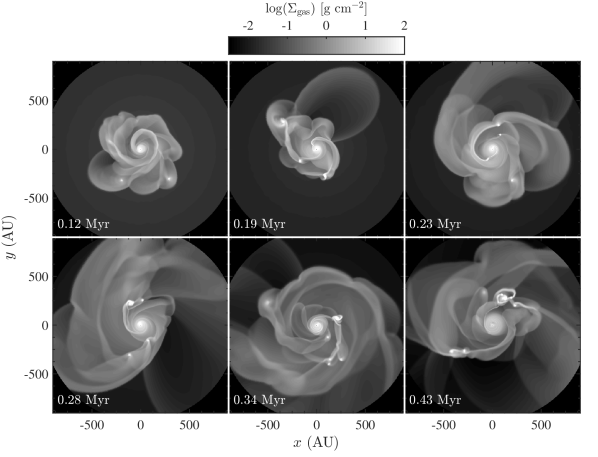
Figure 1 shows $\Sigma_{\rm gas}$ at $t=0.12$, 0.19, 0.23, 0.28, 0.34, and 0.43 Myr in the hydro simulation. Time here is counted from the formation of the protostar (and not from the onset of molecular cloud collapse). A rotating disk component emerges around the protostar at $\sim$0.016 Myr. The disk mass grows from $0.13M_{\odot}$ at t=0.12 Myr to $0.18M_{\odot}$ at t=0.32 Myr; at the meantime the stellar mass increases from $0.37M_{\odot}$ to $0.61M_{\odot}$ (the disk-to-star mass ratio gradually declines with time). Soon after the disk forms, it undergoes GI as driven by ongoing mass loading from the infalling envelope, and fragments. The disk radius increases from $\sim$300 AU at $\sim$0.1 Myr to a maximum of $\sim$700 AU at $\sim$0.3 Myr, and afterwards shrinks. At the 6 epochs, 3–7 fragments are present at stellocentric distances between 100–600 AU. The fragments are generally smaller than 40 AU (0.1$\arcsec$ at 400 pc), and are characterized by surface densities of $\sim$50–2000 g cm^-2. Spiral arms and lobes are present at all epochs. These structures are located at hundreds of AUs from their central stars, and can often extend over $\pi$ in the azimuthal direction. The surface density $\Sigma_{\rm gas}$ of the arms is usually 2.5–20$\times$ higher than the azimuthal average of the background disk at the same radius.

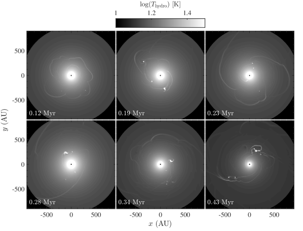
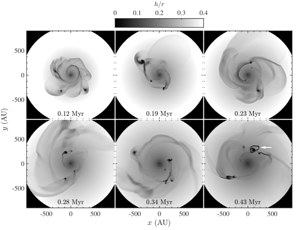
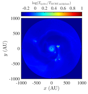
Figures 2 and 3 show $T_{\rm hydro}$ and $h/r$ from the hydro simulation. As derived in Section 2.1, $h$ follows from gravity (from both the central star and disk) balancing pressure $P$ in the vertical direction, where $P$ is set by the hydro disk temperature $T_{\rm hydro}$. Azimuthally averaged $T_{\rm hydro}$ vary from $\sim 80$ K at 10 AU to $\sim 30$ K at 100 AU. In high density regions such as spiral arms and fragments, $T_{\rm hydro}$ increases to up to 230 k because $PdV$ work is done to compress the gas, increasing $h$. On the other hand, in these same overdensities, the local gravity is stronger, decreasing $h$. Our results show that the latter effect dominates the former so that $h$ decreases in high density regions. In most spiral arms, $h$ drops by $\lesssim 20\%$. Such a drop does not necessarily imply that the NIR scattering surface is lower inside arms than outside arms; we will find in Section 3.2 that the scattering surface is actually higher inside the arms because they contain more material. In fragments, the collapse of the local scale height is more dramatic: $h$ drops by factors of 3–30.

3.2 NIR Images

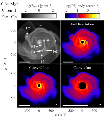
Full resolution and convolved $H$-band PI images of disks at a distance of 400 pc are shown in Figure 4 for all 6 epochs and 2 viewing angles (face-on and $45^{\circ}$ inclination). A detailed comparison between these images at $t=0.34$ Myr and the raw $\Sigma$ image is made in Figure 5. At all epochs the disk is bright and shows complicated structures. We note that the current detection limit (noise level) in NIR PI imaging observations lies at about 0.1 mJy arcsec^-2, if not lower (e.g., Hashimoto et al., 2012; Mayama et al., 2012; Kusakabe et al., 2012; Grady et al., 2013; Follette et al., 2013). This corresponds to the transition between blue (undetectable) and red (detectable) in our NIR color scheme. Our assumed angular resolution ($0.04\arcsec$) is small enough to resolve most spiral arms. As a result, the convolved images are quite similar to the full resolution images.

Most spiral arms appear as prominent bright features, while all fragments appear as depressions in surface brightness (see the 6 fragments marked in Figure 5). These brightness variations are caused by variations in the height of the scattering photosphere, defined as the surface where the optical depth $\tau_{\star}$ to the star is 1. This $\tau_{\star}=1$ surface is determined by $\Sigma$ and $h$. As shown in Juhász et al. (2015), a change in $h$ of at least $20\%$ is required for a structure to be visible in current NIR observations. In our simulated spiral arms, the drop in $h$ due to self-gravity is generally $\lesssim 20\%$ and therefore insignificant; thus, the increase in surface density within the arms pushes the local $\tau_{\star}=1$ surface higher than the surrounding background. Spirals arms are therefore illuminated by the star and appear brighter. By contrast, in fragments, the drop in $h$ due to self-gravity is so significant that these regions are shadowed and appear as holes in NIR scattered light.

Figure 5 also demonstrates the effect of increasing the distance to the object to 1 kpc (roughly the distance to FUors V1735 Cyg and Z CMa). The major spirals at $r\gtrsim 200$ AU remain visible as their physical sizes (in particular their widths) are comparable to the resolution.

The spiral arms appear similar when viewed face-on or at $45^{\circ}$ inclination (see the right two columns of Figure 4). The edge of the nearside of the disk (the bottom side) is not always parallel to the (horizontal) major axis because of variations in disk surface density and scale height. At 0.28 Myr the disk is so asymmetric that even when viewed face-on, it appears nearly one-sided.

3.3 Millimeter Images

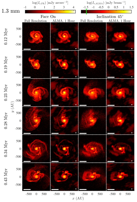
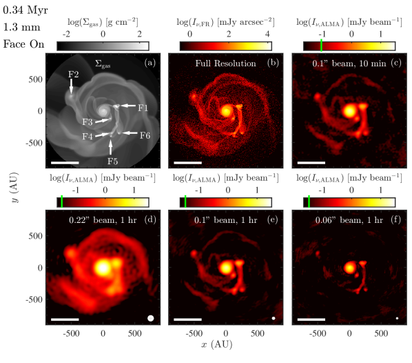
Figure 6 shows full resolution MCRT dust continuum images and simulated ALMA images at 1.3 mm (230 GHz; ALMA band 6). Full resolution images closely trace the surface density at all 6 epochs. Figure 7 provides a closer look at 0.34 Myr, at which time all 6 fragments and major spiral arms identified in $\Sigma$ (panel a) are clearly visible in the full resolution image (panel b). By contrast to the NIR, both spiral arms and fragments in the thermal continuum appear as local maxima, despite the fact that the surface temperatures of the fragments are lower than their surroundings because they are shadowed. Fragments appear bright in the mm because they are optically thick, whereas the ambient disk is optically thin, with vertical optical depths $\lesssim 0.05$.

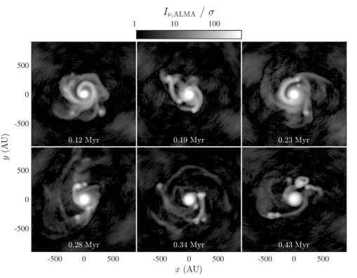
The simulated ALMA images in Figure 6 are produced with array configuration #19 and integration times of 1 hour. The 3$\sigma$ detection limit is 34 $\mu$Jy beam^-1 as calculated by the ALMA sensitivity calculator; in our color scheme this noise floor corresponds to the transition between black (undetected) and red (detected). The synthetic beam size is $\sim$0.1$\arcsec$ (40 AU at 400 pc). Evidently, $0.1\arcsec$ angular resolution is sufficient to resolve most fragments and spiral arms at 400 pc. This can be further illustrated by comparing panels (a) and (e) in Figure 7. Among the 6 fragments in (a), F1, F2, F3, and F6 are clearly visible and distinguishable in (e), while F4 and F5 may be difficult to separate because of their small separation ($\sim$50 AU). The sensitivity is sufficient to detect emission from all major structures out to hundreds of AUs. Figure 8 shows the significance of detections for face-on ALMA images in Figure 6. The masses of fragments, determined using the fragment tracking algorithm of Vorobyov (2013), are 33, 1.0, 2.7, 2.7, 1.9, and 2.5 $M_{\rm J}$, respectively (note that F2 is likely still in the process of formation and will continue growing in the subsequent evolution). All fragments are significantly detected in (c) by at least $40\sigma$, even for the lowest mass fragment F2 of 1$M_{\rm J}$ (also the lowest mass fragment among all epochs). Spiral arms are generally detected at $\gtrsim 10\sigma$ except in the outer regions beyond $\sim$700 AU. Simulated ALMA observations using the parameters underlying Figure 6 recover $>70\%$ of the total mm flux density, as listed in Table LABEL:tab:models. These conclusions are consistent with those of Vorobyov et al. (2013).

The angular resolution and the total integration time are two key parameters in ALMA observations. Figure 7 illustrates the effects of varying these two parameters. Panels (c) and (e) demonstrate the difference between an integration time of 10 minutes (c) and 60 minutes (e), while the resolution is fixed at $0.1\arcsec$. Since the sensitivity is inversely proportional to $\sqrt{\rm integration\ time}$, the noise level in (c) is 2.4 times higher than in (e). The uv sampling of the 10-minute snapshot observation is less complete, and thus side lobes are more prominent in (c). Nevertheless, qualitatively the two panels are quite similar to each other. Fragments F1, F2, F3, F4+F5, and F6 are all significantly detected in (c), with the the least massive fragment F2 (1 $M_{\rm J}$) detected at $17\sigma$. Most spiral arms are also visible in (c), though some are only marginally detected.

Panels (d), (e), and (f) demonstrate the effect of different angular resolutions, achieved by varying the array configuration: (d) has an angular resolution of $0.22\arcsec$ (88 AU at 400 pc, or 2.2 times larger than (e)), while (f) has an angular resolution of $0.06\arcsec$ (24 AU at 400 pc, or $40\%$ smaller than (e)). The integration time is fixed (1 hour) so that their sensitivities are the same in units of mJy beam^-1. The impact of angular resolution is dramatic. In (d), F4, F5, and F6 merge into a larger clump, and F3 is absorbed into the central peak. Spiral arms that are close together also merge to form larger (wider) arms. In (f), although all 6 fragments are resolved by the small beam, their detection significance drops: the weakest source F2 is now a $10\sigma$ detection. At small angular resolution, large-scale structures, such as most spiral arms, are severely resolved out and not visible. As a result, (f) only recovers about $40\%$ of the total flux density in the original full resolution image, while (d) recovers $90\%$ and (e) recovers $72\%$ of the total flux density.

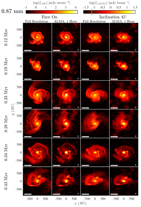
Synthetic ALMA observations at 0.87 mm (345 GHz; ALMA band 7) with $0.1\arcsec$ angular resolution (produced with array configuration #16) are shown in Figure 9. Qualitatively they are similar to the 1.3 mm images.

4 Discussion

4.1 Limitations of Our Models

4.1.1 Gas-Dust Decoupling

Grains in disks are subject to both gravity and gas drag (e.g., Weidenschilling, 1977; Birnstiel et al., 2010). Particles with dimensionless stopping times (a.k.a. Stokes numbers)

$$\tau_{\rm s}=\frac{\pi s\rho_{\rm bulk}}{2\Sigma_{\rm gas}}$$ (19)

approaching unity drift the most quickly toward gas pressure maxima (e.g., Rice et al., 2006; Zhu et al., 2012b). Here $\rho_{\rm bulk}\sim 1$ g/cm³ is the internal bulk density of a grain, and $s$ is the grain size. In our models, big grains with sizes $s\sim 1$ mm at $r\gtrsim 300$ AU can have $\tau_{\rm s}\sim 1$ in low-density inter-arm regions. As a result, our models may be overestimating the surface density of the big grains in low density regions at large distances, as big grains may actually be accumulating in high pressure regions such as spiral arms and fragments. Consequently, we may be underestimating the contrast of the arms and fragments at $r\gtrsim 300$ AU in mm images relative to the surrounding background. Nevertheless, fragments and spiral arms are already detected with high significance in our simulated ALMA images, even without this further concentration; properly taking this effect into account can only enhance their visibilities.

4.1.2 $T_{\rm hydro}$ vs. $T_{\rm MCRT}$

There are two versions of disk temperature in our models. The temperature from our hydro code, $T_{\rm hydro}$, takes into account both radiation from the central star and hydrodynamical processes such as $PdV$ work, viscous and shock heating, and is computed assuming the radiation field is diffusive (Appendix). On the other hand, the MCRT simulation calculates its own temperature, $T_{\rm MCRT}$, which takes into account scattering, absorption, and re-emission of starlight in 3D, but does not include hydrodynamical processes. We expect $T_{\rm MCRT}$ to be more accurate than $T_{\rm hydro}$, everywhere except in regions where hydrodynamical processes are significant, such as inside fragments.

Figure 10 compares the midplane temperatures calculated by the two methods at 0.34 Myr. For the most part, except in fragments, $T_{\rm hydro}$ is lower than $T_{\rm MCRT}$ by $\lesssim 40\%$. Since $h\propto\sqrt{T}$, the inaccuracy in $h$ as propagated from $T_{\rm hydro}$ is expected to be $\lesssim 20\%$. This is not a major source of error; Juhász et al. (2015) found that abrupt changes in $h$ of $\gtrsim 20\%$ are needed to generate discernible effects in current NIR direct imaging observations.

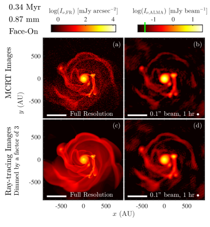
More serious is the discrepancy between temperatures calculated within dense fragments. In fragment centers, $T_{\rm hydro}$ can exceed $T_{\rm MCRT}$ by up to one order of magnitude (Figure 10). The mm-wave thermal fluxes of fragments may therefore be underestimated by our MCRT simulations (the NIR images are more reliable insofar as they depend on vertical scale heights calculated from the more realistic hydro simulation). To assess the error in the mm-wave images, we re-calculate the mm fluxes by inserting the $T_{\rm hydro}$ data into the 3D ray-tracing module of the NATALY radiative transfer code described in Pavlyuchenkov et al. (2011). In these ray-tracing calculations, the disk temperature is set by $T_{\rm hydro}$ and is vertically uniform; the disk is puffed up in the vertical direction in the same way as for the MCRT simulations (see equation 18 and related text); and the (big) dust grains are assumed well mixed with gas with a dust-to-gas mass ratio of $0.9:100$ and an opacity identical to that of big dust in the MCRT simulations. To simulate the inner disk in these ray-tracing calculations, we fill the inner 30 AU with H₂ (number density $10^{10}$ cm^-3 and temperature 50 K).

Figure 11 compares the ray-traced mm images with the MCRT images at 0.34 Myr. The ray-traced images are dimmed by a factor of 3 to fit within the same color scheme used for the MCRT images. Qualitatively the morphology of the disk in the two sets of images are similar, with the peak MCRT fluxes lower by a factor of $\sim$3. This factor of 3 difference in flux is less than the factor of 10 difference in midplane temperature because the fragments are optically thick. In the end, the MCRT and ray-traced images agree that GI-induced spirals and fragments in class 0/I disks at 400 pc can be detected and resolved by ALMA with 1-hour integration times at $0.1\arcsec$ angular resolution.

4.2 Near-Term Prospects for Observing GI in Disks

Disks with $Q<1$ fragment on dynamical, i.e., orbital timescales. Fragments produced by GI may appear quickly, within $\sim$10⁴ years, reducing the disk mass and stabilizing the system against further activity (e.g., Stamatellos et al., 2011). Thus GI may be a short-lived phenomenon that is difficult to observe. However, GI can be recurring and prolonged if fresh gas is supplied to the disk from its natal envelope, on timescales up to a few $\times$ 10⁵ yr. Similarly, individual fragments may be lost (or downsized) as they get shredded by tidal forces, migrate into the central star, or get ejected from the system (e.g., Vorobyov & Basu, 2010a; Boley et al., 2010; Nayakshin, 2010; Machida et al., 2011b; Zhu et al., 2012a; Basu & Vorobyov, 2012; Tsukamoto et al., 2015); but fragments can be recurring as well.

At mm wavelengths, envelopes do not much obscure our view of embedded disks. Contamination from envelope emission is on the order of $\sim$30% in dust continuum emissions for class 0 sources, and $\sim$10% for class I sources (Jørgensen et al., 2009). At NIR wavelengths, the situation is more challenging, as disks can be heavily extincted by envelopes. Our MCRT calculations ignore envelopes and should therefore be applied to systems in kind (i.e., late stage I), or to disks with envelopes viewed nearly face-on with large opening angles for their bipolar cavities.

We may search for GI in (1) disks with $M_{\rm disk}\gtrsim 0.3M_{\star}$, and (2) disks undergoing accretion outbursts. Millimeter observations of class 0/I disks have confirmed the presence of large ($>100$ AU) disks in a few systems (Tobin et al., 2015; Yen et al., 2015a; Choi et al., 2007), and have suggested a number of candidates with $M_{\rm disk}\gtrsim 0.1M_{\odot}$ (Jørgensen et al., 2007, 2009; Eisner et al., 2008), modulo the usual uncertainties in gas-to-dust ratio and dust opacity (e.g., Dunham et al., 2014). A particularly interesting case is HL Tau (ALMA Partnership et al., 2015), which has an estimated disk mass of about $0.1M_{\odot}$, or $20\%$ of the stellar mass (Greaves et al., 2008; Kwon et al., 2011). Jin et al. (2016) have suggested that the disk is marginally GI-unstable, and that disk self-gravity facilitates the formation of gaps by relatively low-mass planets (e.g., Dong et al., 2015b; Dipierro et al., 2015).

Young stellar objects undergoing accretion outbursts, such as FUors and EXors, are thought to be GI-unstable disks. Measuring their disk masses (e.g., Liu et al., 2016a) will be crucial for validating this interpretation. These objects are excellent targets for future high angular resolution observations to detect GI-induced spiral arms. In pioneering work, Liu et al. (2016b) directly imaged spiral arms and streams in four FUors with Subaru. The structures seen in the Subaru images resemble those in our NIR model images, supporting the idea that FUors are GI-unstable protostellar/protoplanetary disks (e.g., Vorobyov & Basu, 2005, 2010b, 2015).

What are the implications if the clumps and spiral arms predicted by our synthetic images are not seen?

1. If mm continuum observations do not detect the disk while NIR imaging observations do, it may imply that we have overestimated the mm-wave dust opacity. In our model, the mm opacity of the big grains (up to 1 mm in size) is about 13 cm² g^-1, consistent with the results found by Draine (2006) to within factors of a few for grains of similar sizes, and about two orders of magnitude higher than the corresponding opacity for ISM grains. If substantial grain growth has not occurred in class 0/I disks, the mm fluxes of our models could be overestimated by up to two orders of magnitude.

2. If mm observations reveal no Keplerian disk beyond a few tens of AU (e.g., as suggested in B335 by Yen et al. 2015b), it may imply the action of strong magnetic braking (Krasnopolsky & Königl, 2002; Li et al., 2011; Machida et al., 2011a), enabled perhaps by very small grains $\sim$10–100 $\AA$ in size that can couple magnetic fields to matter (Zhao et al., 2016). NIR imaging observations may not see these small disks at all if they lie inside the inner working angle (a few tens of AU at a few hundred pc).

3. If observations at both NIR and mm wavelengths show a large but featureless (i.e., axisymmetric) disk on scales $\gtrsim 100$ AU, the disk may either be insufficiently massive to be GI-unstable (equation 1 is not satisfied) or cool on timescales so long that GI-induced activity is too anemic to be detected ($t_{\rm cool}\Omega\gg 1$; cf. equation 2).

5 Summary

Using 2+1D hydrodynamics simulations, we modeled the formation and subsequent evolution of a protostellar disk starting from a molecular cloud core, for times ranging up $0.5$ Myr. The disk, fed by an infalling envelope, experiences gravitational instability. It develops large-scale spiral arms, portions of which fragment. The resulting density structures at six epochs spanning 0.12–0.43 Myr after the formation of the protostar are transformed into NIR scattered light images and simulated ALMA dust continuum maps using a 3D Monte Carlo radiative transfer code. Our main conclusions are as follows.

1. As long as they are not obscured by an intervening envelope, GI-induced spiral arms viewed at modest inclinations ($\lesssim 45^{\circ}$) are visible at distances up to 1 kpc with the current suite of NIR imaging instrumentation (including Gemini/GPI, VLT/SPHERE, and Subaru/HiCIAO/SCExAO).

2. The spiral arms and streamers in four FU Ori objects recently revealed by Subaru (Liu et al., 2016a, b) resemble GI-induced structures in our models, supporting the idea that FUors represent GI-unstable disks (e.g., Vorobyov & Basu, 2005, 2010b, 2015).

3. Clumps formed by disk fragmentation have such small vertical scale heights that they are shadowed and appear as surface brightness depressions in NIR scattered light.

4. Both spiral arms and fragments in GI-unstable disks can be resolved and readily detected (by $\sim$10$\sigma$ for arms and by $\gtrsim 40\sigma$ for fragments) in ALMA dust continuum observations of sources at 400 pc with an angular resolution of $0.1\arcsec$ and one-hour integration times. The minimum detectable fragment mass is $\sim$1 $M_{\rm J}$ under these observing conditions.

Future work can focus on developing a 3D code that treats the hydrodynamics and radiative transfer of self-gravitating disks self-consistently, and on allowing dust and gas to slip past each other. Although our work is deficient in these regards, it points robustly to the observability of gravitational instability in protostellar disks, given the powerful instrumentation available today.

Appendix: Relation between the emergent radiative flux and midplane temperature

Let us consider a locally isothermal disk in vertical hydrostatic equilibrium. In the plane-parallel approximation, the thermal structure of the disk can be described by the following system of radiative transfer moment equations:

$$\frac{dF}{dz}=c\rho\kappa_{P}(B-E)$$ (20)

$$\frac{c}{3}\frac{dE}{dz}=-\rho\kappa_{R}F,$$ (21)

where $c$ is the speed of light, $\rho$ the gas volume density, $\kappa_{P}$ and $\kappa_{R}$ the Planck and Rosseland mean opacities, $E$ the radiation energy density, $F$ the radiative flux, $B=aT^{4}$ the radiation energy density in thermal equilibrium ($a=4\sigma/c$ the radiation constant, $T$ the gas temperature). Equation (20) indicates that the radiative flux $F$ depends on the difference between emission and absorption in the vertical column of the disk. Equation (21) expresses the relation between the radiative flux and radiation energy density in the Eddington approximation.

This system of equations is closed with the following equation:

$$\frac{dF}{dz}=\rho S,$$ (22)

which states that the radiative flux $F$ is actually produced by a non-radiative heating source $\rho S$. Here, $S$ is defined as the heating rate per unit mass. It is convenient to rewrite these equations using the integrated surface density from the midplane to a given vertical distance $z$, $\overline{\Sigma}(z)=\int\limits_{0}^{z}\rho(z^{\prime})dz^{\prime}$. We note that $\overline{\Sigma}(h)\equiv\Sigma_{1/2}\equiv\Sigma/2$ is the gas surface density from the midplane to the disk surface. The resulting equations take the following form:

$$c\kappa_{P}(B-E)=S$$ (23)

$$\frac{c}{3}\frac{dE}{d\overline{\Sigma}}=-\kappa_{R}F$$ (24)

$$\frac{dF}{d\overline{\Sigma}}=S.$$ (25)

We now assume that $S$ is constant in the vertical direction, meaning that $\rho S$ is proportional to the mass in the vertical column of the disk. Given that the radiative flux is zero at the midplane, the integration of equation (25) yields:

$$F=S\overline{\Sigma}.$$ (26)

After substituting equation (26) into equation (24) and integrating equation (24) from the midplane to the surface of the disk, we obtain:

$$E(\Sigma_{1/2})=E(0)-\dfrac{3\kappa_{R}S}{2c}\Sigma_{1/2}^{2},$$ (27)

where $E(0)$ and $E(\Sigma_{1/2})$ are the radiation energy densities at the midplane and at the disk surface, correspondingly. Now, let us adopt the following boundary condition at the disk surface:

$$F(\Sigma_{1/2})=\frac{1}{2}cE(\Sigma_{1/2}),$$ (28)

which assumes that radiation escapes from the disk surface isotropically. Using equation (26) we obtain:

$$S=\frac{cE(\Sigma_{1/2})}{2\Sigma_{1/2}}.$$ (29)

Finally, substituting $S$ in equation (27), we obtain the relation between the radiation energy density at the disk surface surface and midplane:

$$E(\Sigma_{1/2})=\frac{E(0)}{1+\dfrac{3}{4}\tau_{\rm R}},$$ (30)

where $\tau_{\rm R}=\kappa_{\rm R}\Sigma_{1/2}$ is the the Rosseland optical depth from the midplane to the disk surface. Using equations (23) and (29), $E(0)$ can be rewritten in the following form:

$$E(0)=B(0)-\frac{E(\Sigma_{1/2})}{2\tau_{\rm P}},$$ (31)

where $\tau_{P}=\kappa_{P}\Sigma_{1/2}$ is the Planck optical depth from the midplane to the disk surface and $B(0)$ the Planck radiation energy density at the midplane. Substituting equation (31) into equation (30), we obtain:

$$E(\Sigma_{1/2})=\frac{2\tau_{\rm P}}{1+2\tau_{\rm P}+\dfrac{3}{2}\tau_{\rm R}\tau_{\rm P}}B(0)$$ (32)

Using the boundary condition (28) and noting that $\sigma=ca/4$ we finally obtain the relation between the midplane temperature and the radiative flux emerging from the disk surface:

$$F(\Sigma_{1/2})=\frac{4\tau_{\rm P}\sigma T_{\rm hydro}^{4}}{1+2\tau_{\rm P}+\dfrac{3}{2}\tau_{\rm R}\tau_{\rm P}},$$ (33)

where $T_{\rm hydro}$ is the midplane temperature in hydro simulations.

Table 1: Models

Time	$M_{\rm disk}$	$M_{\star}$	$T_{\star}$	$L_{\star}$	$\dot{M}$	$F_{\rm 0^{\circ},FR}$	$F_{\rm 0^{\circ},ALMA}$	$F_{\rm 45^{\circ},FR}$	$F_{\rm 45^{\circ},ALMA}$
Myr	$M_{\odot}$	$M_{\odot}$	K	$L_{\odot}$	$M_{\odot}$ yr-1	mJy	mJy	mJy	mJy
0.12	0.135	0.366	4270	5.15	$1.1\times 10^{-6}$	152	112	136	98
0.19	0.190	0.463	4100	5.5	$1.3\times 10^{-6}$	154	122	131	104
0.23	0.203	0.514	4050	5.2	$2.0\times 10^{-6}$	191	133	169	115
0.28	0.209	0.571	3830	7.2	$1.8\times 10^{-6}$	176	130	153	110
0.34	0.171	0.615	3800	4.2	$8.0\times 10^{-6}$	117	84	101	67
0.43	0.179	0.655	3800	4	$8.0\times 10^{-6}$	107	71	99	65

Figure 1: Model gas surface densities. The disk rotation is counterclockwise.

Figure 2: Temperature in the hydro models $T_{\rm hydro}$.

Figure 3: Disk aspect ratios $h/r$ in the hydro models.

Figure 4: $H$-band PI images of the disk viewed face-on (left two columns) and at an inclination of $45^{\circ}$ (right two columns; the side of the disk nearest the observer is located at the bottom of each panel, and the major axis is horizontal). The $1^{\rm st}$ and $3^{\rm rd}$ columns are at full resolution, while the $2^{\rm nd}$ and $4^{\rm th}$ columns contain images convolved with a Gaussian PSF with a FWHM of 0.04$\arcsec$ (angular resolution of an 8-m telescope at $H$-band) at a source distance of 400 pc. Current detection limits (noise levels) for NIR PI imaging are $\sim$0.1 mJy arcsec^-2, corresponding to the transition between red (detected) and blue (undetected). Each panel masks out an inner working angle of $0.15\arcsec$. The scale bar at the lower left is $1\arcsec$ long. See Section 3.2 for details.

Figure 5: Comparing gas surface density to NIR surface brightness at 0.34 Myr, and the effect of source distance. The bottom two panels are convolved images assuming a distance of 400 pc (left) and 1 kpc (right). The locations of 6 fragments are marked in the $\Sigma_{\rm gas}$ map. The central $0.15\arcsec$ in each NIR image is masked out, and the scale bar is $1\arcsec$. Current detection limits (noise levels) for NIR PI imaging are $\sim$0.1 mJy arcsec^-2, marked as the green tick on the color bar. See Section 3.2 for details.

Figure 6: ALMA band 6 (1.3 mm) images at viewing angles of $0^{\circ}$ (left two columns) and $45^{\circ}$ (right two columns; the side of the disk nearest the observer is oriented toward the bottom of each panel, and the major axis is horizontal). The $1^{\rm st}$ and $3^{\rm rd}$ columns are at full resolution and use the color bar on the left. The $2^{\rm nd}$ and $4^{\rm th}$ columns, using the color bar on the right, are simulated one-hour integrations with ALMA in array configuration #19 (angular resolution $\sim$0.1$\arcsec$; the beam is indicated in the lower right corner). The source distance is 400 pc. The $3\sigma$ detection limit in simulated ALMA images is 0.034 mJy beam^-1 and is marked by the green tick on the color bar. The horizontal scale bar indicates $1\arcsec$. See Section 3.3 for details.

Figure 7: The effects of integration time and angular resolution on ALMA observations. Panels (c), (d), (e), and (f) are simulated ALMA observations based on the full resolution synthetic MCRT image in (b). The source is at 400 pc. The array configurations used in the ALMA simulator are #13 (d; angular resolution $\sim$$0.22\arcsec$), #19 (b, e; angular resolution $\sim$$0.1\arcsec$), and #22 (d; angular resolution $\sim$$0.06\arcsec$). The difference between (c) and (e) is integration time: 10 minutes vs. 1 hour. The $3\sigma$ detection limit in each simulated ALMA image is marked as a green tick on the color scale. See Section 3.3 for details.

Figure 8: The statistical significance of detections in simulated face-on ALMA Band 6 observations (see also Figure 6), in units of $\sigma=0.011$ mJy beam^-1. See Section 3.3 for details.

Figure 9: Same as Figure 6, but for ALMA Band 7 (0.87 mm), array configuration #16, and a one-hour integration time.

Figure 10: Log$({T_{\rm hydro}/T_{\rm MCRT,midplane}})$ at 0.34 Myr. The difference between the two temperatures is $\lesssim 40$% everywhere except at the centers of fragments, where $T_{\rm hydro}$ can be up to one order of magnitude higher than $T_{\rm MCRT,midplane}$. See Section 4.1 for details.

Figure 11: Comparison between MCRT mm-wave images (top row) and mm-wave images produced by ray-tracing calculations with NATALY (bottom row). The source is at 400 pc distance. The left panels show full resolution images, while the right panels show simulated one-hour ALMA observations with array configuration #19 (resolution $\sim 0.1\arcsec$). The ray-traced images are dimmed by a factor of 3 to fit within the color scheme adopted for the MCRT images. See Section 4.1 for details.

References

- ALMA Partnership et al. (2015) ALMA Partnership, et al. 2015, ApJ, 808, L3
- Andre & Montmerle (1994) Andre, P., & Montmerle, T. 1994, ApJ, 420, 837
- Andre et al. (1993) Andre, P., Ward-Thompson, D., & Barsony, M. 1993, ApJ, 406, 122
- Audard et al. (2014) Audard, M., et al. 2014, Protostars and Planets VI, 387
- Bae et al. (2014) Bae, J., Hartmann, L., Zhu, Z., & Nelson, R. P. 2014, ApJ, 795, 61
- Baraffe & Chabrier (2010) Baraffe, I., & Chabrier, G. 2010, A&A, 521, A44
- Baraffe et al. (2012) Baraffe, I., Vorobyov, E., & Chabrier, G. 2012, ApJ, 756, 118
- Basu (1997) Basu, S. 1997, ApJ, 485, 240
- Basu & Vorobyov (2012) Basu, S., & Vorobyov, E. I. 2012, ApJ, 750, 30
- Beuzit et al. (2008) Beuzit, J.-L., et al. 2008, in Society of Photo-Optical Instrumentation Engineers (SPIE) Conference Series, Vol. 7014, Society of Photo-Optical Instrumentation Engineers (SPIE) Conference Series
- Binney & Tremaine (1987) Binney, J., & Tremaine, S. 1987, Galactic dynamics (Princeton, NJ, Princeton University Press, 1987, 747 p.)
- Birnstiel et al. (2010) Birnstiel, T., Dullemond, C. P., & Brauer, F. 2010, A&A, 513, A79
- Boley et al. (2010) Boley, A. C., Hayfield, T., Mayer, L., & Durisen, R. H. 2010, Icarus, 207, 509
- Boss (1997) Boss, A. P. 1997, Science, 276, 1836
- Bowler et al. (2013) Bowler, B. P., Liu, M. C., Shkolnik, E. L., & Dupuy, T. J. 2013, ApJ, 774, 55
- Caceres et al. (2015) Caceres, C., et al. 2015, ApJ, 806, L22
- Canovas et al. (2015) Canovas, H., et al. 2015, A&A, 578, L1
- Chiang et al. (2012) Chiang, H.-F., Looney, L. W., & Tobin, J. J. 2012, ApJ, 756, 168
- Choi et al. (2007) Choi, M., Tatematsu, K., Park, G., & Kang, M. 2007, ApJ, 667, L183
- Cossins et al. (2010) Cossins, P., Lodato, G., & Testi, L. 2010, MNRAS, 407, 181
- Dapp & Basu (2009) Dapp, W. B., & Basu, S. 2009, MNRAS, 395, 1092
- Dipierro et al. (2014) Dipierro, G., Lodato, G., Testi, L., & de Gregorio Monsalvo, I. 2014, MNRAS, 444, 1919
- Dipierro et al. (2015) Dipierro, G., Price, D., Laibe, G., Hirsh, K., Cerioli, A., & Lodato, G. 2015, MNRAS, 453, L73
- Dong et al. (2015a) Dong, R., Hall, C., Rice, K., & Chiang, E. 2015a, ApJ, 812, L32
- Dong et al. (2012) Dong, R., et al. 2012, ApJ, 750, 161
- Dong et al. (2015b) Dong, R., Zhu, Z., & Whitney, B. 2015b, ApJ, 809, 93
- Douglas et al. (2013) Douglas, T. A., Caselli, P., Ilee, J. D., Boley, A. C., Hartquist, T. W., Durisen, R. H., & Rawlings, J. M. C. 2013, MNRAS, 433, 2064
- Draine (2006) Draine, B. T. 2006, ApJ, 636, 1114
- Dunham et al. (2014) Dunham, M. M., Vorobyov, E. I., & Arce, H. G. 2014, MNRAS, 444, 887
- Eisner et al. (2008) Eisner, J. A., Plambeck, R. L., Carpenter, J. M., Corder, S. A., Qi, C., & Wilner, D. 2008, ApJ, 683, 304
- Follette et al. (2013) Follette, K. B., et al. 2013, ApJ, 767, 10
- Gammie (2001) Gammie, C. F. 2001, ApJ, 553, 174
- Goldreich & Lynden-Bell (1965) Goldreich, P., & Lynden-Bell, D. 1965, MNRAS, 130, 97
- Grady et al. (2013) Grady, C. A., et al. 2013, ApJ, 762, 48
- Greaves et al. (2008) Greaves, J. S., Richards, A. M. S., Rice, W. K. M., & Muxlow, T. W. B. 2008, MNRAS, 391, L74
- Hartmann et al. (1998) Hartmann, L., Calvet, N., Gullbring, E., & D’Alessio, P. 1998, ApJ, 495, 385
- Hashimoto et al. (2012) Hashimoto, J., et al. 2012, ApJ, 758, L19
- Henyey & Greenstein (1941) Henyey, L. G., & Greenstein, J. L. 1941, ApJ, 93, 70
- Herbig (2008) Herbig, G. H. 2008, AJ, 135, 637
- Hinkley et al. (2009) Hinkley, S., et al. 2009, ApJ, 701, 804
- Jin et al. (2016) Jin, S., Li, S., Isella, A., Li, H., & Ji, J. 2016, ArXiv e-prints
- Jørgensen et al. (2007) Jørgensen, J. K., et al. 2007, ApJ, 659, 479
- Jørgensen et al. (2009) Jørgensen, J. K., van Dishoeck, E. F., Visser, R., Bourke, T. L., Wilner, D. J., Lommen, D., Hogerheijde, M. R., & Myers, P. C. 2009, A&A, 507, 861
- Jovanovic et al. (2015) Jovanovic, N., et al. 2015, PASP, 127, 890
- Juhász et al. (2015) Juhász, A., Benisty, M., Pohl, A., Dullemond, C. P., Dominik, C., & Paardekooper, S.-J. 2015, MNRAS, 451, 1147
- Kim et al. (1994) Kim, S.-H., Martin, P. G., & Hendry, P. D. 1994, ApJ, 422, 164
- Krasnopolsky & Königl (2002) Krasnopolsky, R., & Königl, A. 2002, ApJ, 580, 987
- Kratter et al. (2010) Kratter, K. M., Murray-Clay, R. A., & Youdin, A. N. 2010, ApJ, 710, 1375
- Kraus et al. (2015) Kraus, A. L., Andrews, S. M., Bowler, B. P., Herczeg, G., Ireland, M. J., Liu, M. C., Metchev, S., & Cruz, K. L. 2015, ApJ, 798, L23
- Kraus & Ireland (2012) Kraus, A. L., & Ireland, M. J. 2012, ApJ, 745, 5
- Kusakabe et al. (2012) Kusakabe, N., et al. 2012, ApJ, 753, 153
- Kuzuhara et al. (2013) Kuzuhara, M., et al. 2013, ApJ, 774, 11
- Kwon et al. (2011) Kwon, W., Looney, L. W., & Mundy, L. G. 2011, ApJ, 741, 3
- Li et al. (2011) Li, Z.-Y., Krasnopolsky, R., & Shang, H. 2011, ApJ, 738, 180
- Liu et al. (2016a) Liu, H. B., et al. 2016a, ApJ, 816, L29
- Liu et al. (2016b) —. 2016b, ArXiv e-prints
- Machida et al. (2011a) Machida, M. N., Inutsuka, S.-I., & Matsumoto, T. 2011a, PASJ, 63, 555
- Machida et al. (2011b) Machida, M. N., Inutsuka, S.-i., & Matsumoto, T. 2011b, ApJ, 729, 42
- Macintosh et al. (2008) Macintosh, B. A., et al. 2008, in Society of Photo-Optical Instrumentation Engineers (SPIE) Conference Series, Vol. 7015, Society of Photo-Optical Instrumentation Engineers (SPIE) Conference Series
- Masunaga & Inutsuka (2000) Masunaga, H., & Inutsuka, S.-i. 2000, ApJ, 531, 350
- Mayama et al. (2012) Mayama, S., et al. 2012, ApJ, 760, L26
- Mayer et al. (2016) Mayer, L., Peters, T., Pineda, J. E., & Wadsley, J. 2016, ArXiv e-prints
- Meru & Bate (2011) Meru, F., & Bate, M. R. 2011, MNRAS, 411, L1
- Miotello et al. (2014) Miotello, A., Testi, L., Lodato, G., Ricci, L., Rosotti, G., Brooks, K., Maury, A., & Natta, A. 2014, A&A, 567, A32
- Nayakshin (2010) Nayakshin, S. 2010, MNRAS, 408, L36
- Pavlyuchenkov et al. (2011) Pavlyuchenkov, Y. N., Wiebe, D. S., Fateeva, A. M., & Vasyunina, T. S. 2011, Astronomy Reports, 55, 1
- Perrin et al. (2004) Perrin, M. D., Graham, J. R., Kalas, P., Lloyd, J. P., Max, C. E., Gavel, D. T., Pennington, D. M., & Gates, E. L. 2004, Science, 303, 1345
- Pohl et al. (2015) Pohl, A., Pinilla, P., Benisty, M., Ataiee, S., Juhász, A., Dullemond, C. P., Van Boekel, R., & Henning, T. 2015, MNRAS, 453, 1768
- Rafikov (2005) Rafikov, R. R. 2005, ApJ, 621, L69
- Rafikov (2009) —. 2009, ApJ, 704, 281
- Rice et al. (2003) Rice, W. K. M., Armitage, P. J., Bate, M. R., & Bonnell, I. A. 2003, MNRAS, 339, 1025
- Rice et al. (2006) Rice, W. K. M., Armitage, P. J., Wood, K., & Lodato, G. 2006, MNRAS, 373, 1619
- Rice et al. (2005) Rice, W. K. M., Lodato, G., & Armitage, P. J. 2005, MNRAS, 364, L56
- Rosenfeld et al. (2014) Rosenfeld, K. A., Chiang, E., & Andrews, S. M. 2014, ApJ, 782, 62
- Semenov et al. (2003) Semenov, D., Henning, T., Helling, C., Ilgner, M., & Sedlmayr, E. 2003, A&A, 410, 611
- Shi & Chiang (2014) Shi, J.-M., & Chiang, E. 2014, ApJ, 789, 34
- Stamatellos et al. (2011) Stamatellos, D., Maury, A., Whitworth, A., & André, P. 2011, MNRAS, 413, 1787
- Stamatellos & Whitworth (2009) Stamatellos, D., & Whitworth, A. P. 2009, MNRAS, 392, 413
- Takahashi & Inutsuka (2014) Takahashi, S. Z., & Inutsuka, S.-i. 2014, ApJ, 794, 55
- Tobin et al. (2015) Tobin, J. J., et al. 2015, ApJ, 805, 125
- Tsukamoto et al. (2013) Tsukamoto, Y., Machida, M. N., & Inutsuka, S.-i. 2013, MNRAS, 436, 1667
- Tsukamoto et al. (2015) Tsukamoto, Y., Takahashi, S. Z., Machida, M. N., & Inutsuka, S. 2015, MNRAS, 446, 1175
- Vorobyov (2013) Vorobyov, E. I. 2013, A&A, 552, A129
- Vorobyov & Basu (2005) Vorobyov, E. I., & Basu, S. 2005, ApJ, 633, L137
- Vorobyov & Basu (2006) —. 2006, ApJ, 650, 956
- Vorobyov & Basu (2009) —. 2009, MNRAS, 393, 822
- Vorobyov & Basu (2010a) —. 2010a, ApJ, 714, L133
- Vorobyov & Basu (2010b) —. 2010b, ApJ, 719, 1896
- Vorobyov & Basu (2015) —. 2015, ApJ, 805, 115
- Vorobyov et al. (2013) Vorobyov, E. I., Zakhozhay, O. V., & Dunham, M. M. 2013, MNRAS, 433, 3256
- Weidenschilling (1977) Weidenschilling, S. J. 1977, MNRAS, 180, 57
- White (1979) White, R. L. 1979, ApJ, 229, 954
- Whitney et al. (2013) Whitney, B. A., Robitaille, T. P., Bjorkman, J. E., Dong, R., Wolff, M. J., Wood, K., & Honor, J. 2013, ApJS, 207, 30
- Yen et al. (2015a) Yen, H.-W., Koch, P. M., Takakuwa, S., Ho, P. T. P., Ohashi, N., & Tang, Y.-W. 2015a, ApJ, 799, 193
- Yen et al. (2015b) Yen, H.-W., Takakuwa, S., Koch, P. M., Aso, Y., Koyamatsu, S., Krasnopolsky, R., & Ohashi, N. 2015b, ApJ, 812, 129
- Zhao et al. (2016) Zhao, B., Caselli, P., Li, Z.-Y., Krasnopolsky, R., Shang, H., & Nakamura, F. 2016, ArXiv e-prints
- Zhu et al. (2009) Zhu, Z., Hartmann, L., Gammie, C., & McKinney, J. C. 2009, ApJ, 701, 620
- Zhu et al. (2012a) Zhu, Z., Hartmann, L., Nelson, R. P., & Gammie, C. F. 2012a, ApJ, 746, 110
- Zhu et al. (2012b) Zhu, Z., Nelson, R. P., Dong, R., Espaillat, C., & Hartmann, L. 2012b, ApJ, 755, 6
- Zhu et al. (2015) Zhu, Z., Dong, R., Stone, J. M., & Rafikov, R. R. 2015, ApJ, 813, 88