Rungs 1 to 4 of DFT Jacob’s ladder: extensive test on the lattice constant, bulk modulus, and cohesive energy of solids

Abstract

A large panel of old and recently proposed exchange-correlation functionals belonging to rungs 1 to 4 of Jacob’s ladder of density functional theory are tested (with and without a dispersion correction term) for the calculation of the lattice constant, bulk modulus, and cohesive energy of solids. Particular attention will be paid to the functionals MGGA_MS2 [J. Sun et al., J. Chem. Phys. 138, 044113 (2013)], mBEEF [J. Wellendorff et al., J. Chem. Phys. 140, 144107 (2014)], and SCAN [J. Sun et al., Phys. Rev. Lett. 115, 036402 (2015)] that are approximations of the meta-generalized gradient type and were developed with the goal to be universally good. Another goal is also to determine for which semilocal functionals and groups of solids it is beneficial (or not necessary) to use the Hartree-Fock exchange or a dispersion correction term.

I Introduction

Starting in the mid 1980’s,Becke (1986); Perdew and Wang (1986) there has been a constantly growing interest in the development of exchange-correlation (xc) functionals $E_{\text{xc}}=E_{\text{x}}+E_{\text{c}}$ in the Kohn-Sham (KS) density functional theory (DFT), Hohenberg and Kohn (1964); Kohn and Sham (1965) and the number of functionals that have been proposed so far is rather huge (see, e.g., Refs. Cohen et al., 2012; Burke, 2012; Becke, 2014; Jones, 2015 for recent reviews). This is understandable since KS-DFT is the most used method for the theoretical modeling of solids, surfaces, and molecules at the quantum level, and the accuracy of a KS-DFT calculation depends to a large extent on the chosen approximation for $E_{\text{xc}}$. Over the years, the degree of sophistication of the functionals (and their accuracy) has increased and most of the functionals belong to one of the rungs of Jacob’s ladder.Perdew and Schmidt (2001); Perdew et al. (2005) On the first three rungs there are the so-called semilocal (SL) approximations which consist of a single integral for $E_{\text{xc}}$,

$$E_{\text{xc}}^{\text{SL}}=\int\epsilon_{\text{xc}}(\mathbf{r})d^{3}r,$$ (1)

and where $\epsilon_{\text{xc}}$, the exchange-correlation energy density per volume, is a function of (a) the electron density $\rho=\sum_{i=1}^{N}\left|\psi_{i}\right|^{2}$ in the local density approximation (LDA, first rung), (b) $\rho$ and its first derivative $\nabla\rho$ in the generalized gradient approximation (GGA, second rung), and (c) $\rho$, $\nabla\rho$, and the kinetic-energy (KE) density $t=\left(1/2\right)\sum_{i=1}^{N}\nabla\psi_{i}^{*}\cdot\nabla\psi_{i}$ and/or $\nabla^{2}\rho$ in the meta-GGA approximation (MGGA, third rung). On the fourth rung there are the functionals which make use of the (short-range, SR) Hartree-Fock (HF) exchange, like the hybrid functionals Becke (1993)

$$E_{\text{xc}}^{\text{hybrid}}=E_{\text{xc}}^{\text{SL}}+\alpha_{\text{x}}\left(E_{\text{x}}^{\text{(SR-)HF}}-E_{\text{x}}^{\text{(SR-)SL}}\right),$$ (2)

where $\alpha_{\text{x}}$ ($\in[0,1]$) is the fraction of HF exchange energy $E_{\text{x}}^{\text{(SR-)HF}}$ which is a double integral:

$$E_{\text{x}}^{\text{(SR-)HF}} = -\frac{1}{2}\sum_{i=1}^{N}\sum_{j=1}^{N}\delta_{\sigma_{i}\sigma_{j}}\int\int\psi_{i}^{*}(\mathbf{r})\psi_{j}(\mathbf{r})$$ (3)

$$\times v\left(\left|\mathbf{r}-\mathbf{r^{\prime}}\right|\right)\psi_{j}^{*}(\mathbf{r^{\prime}})\psi_{i}(\mathbf{r^{\prime}})d^{3}rd^{3}r^{\prime},$$

where the indices $i$ and $j$ run over the occupied orbitals and $v$ is the Coulomb potential $1/\left|\mathbf{r}-\mathbf{r^{\prime}}\right|$ or only the SR part of itBylander and Kleinman (1990); Heyd et al. (2003) (i.e., a screened potential). On the fifth rung of Jacob’s ladder there are the functionals which utilize all (occupied and unoccupied) orbitals, like the random phase approximation (RPA, see, e.g., Refs. Harl and Kresse, 2008; Olsen and Thygesen, 2013).

The functionals of the first four rungs have been extremely successful in describing the properties of all kinds of electronic systems, ranging from atoms to solids.Cohen et al. (2012); Burke (2012); Becke (2014) However, a well-known problem common to all these functionals is that the long-range London dispersion interactions (always attractive and resulting from the interaction between non-permanent multipoles) are formally not included. In the case of two nonoverlapping spherical atoms, these functionals give an interaction energy of strictly zero, which is not the case in reality because of the attractive London dispersion interactions. As a consequence, the results obtained with the semilocal and hybrid functionals on systems where the London dispersion interactions play a major role can be qualitatively wrong.Klimeš and Michaelides (2012) Nevertheless, as underlined in Ref. Zhao and Truhlar, 2005, at equilibrium geometry the overlap between two interacting entities is not zero, such that a semilocal or hybrid xc-functional can eventually lead to a non-zero contribution to the interaction energy and therefore, possibly useful results (see, e.g., Ref. Sun et al., 2013a). In order to improve the reliability of KS-DFT calculations for such systems, functionals including the dispersion interactions in their construction were proposed. A simple and widely used method consists of adding to the semilocal or hybrid functional an atom-pairwise (PW) term of the form

$$E_{\text{c,disp}}^{\text{PW}}=-\sum_{A<B}\sum_{n=6,8,10,\ldots}f_{n}^{\text{damp}}(R_{AB})\frac{C_{n}^{AB}}{R_{AB}^{n}},$$ (4)

where $C_{n}^{AB}$ are the dispersion coefficients for the atom pair $A$ and $B$ separated by the distance $R_{AB}$ and $f_{n}^{\text{damp}}$ is a damping function preventing Eq. (4) to become too large for small $R_{AB}$. The coefficients $C_{n}^{AB}$ can be either precomputed (see, e.g., Refs. Wu et al., 2001; Wu and Yang, 2002; Hasegawa and Nishidate, 2004; Grimme, 2004, 2006; Ortmann et al., 2006) or calculated using properties of the system like the atomic positions or the electron density (see, e.g., Refs. Becke and Johnson, 2005; Tkatchenko and Scheffler, 2009; Grimme et al., 2010). The other group of well-known methods accounting explicitly of dispersion interactions consists of adding to $E_{\text{xc}}^{\text{SL/hybrid}}$ a nonlocal (NL, in the sense of being a double integral) term of the form Dion et al. (2004)

$$E_{\text{c,disp}}^{\text{NL}}=\frac{1}{2}\int\int\rho(\textbf{r})\Phi\left(\textbf{r},\textbf{r}^{\prime}\right)\rho(\textbf{r}^{\prime})d^{3}rd^{3}r^{\prime},$$ (5)

where the kernel $\Phi$ depends on $\rho$ and $\nabla\rho$ at r and $\textbf{r}^{\prime}$ as well as on $\left|\textbf{r}-\textbf{r}^{\prime}\right|$. Several functionals of the form of Eq. (5) are available in the literatureDion et al. (2004); Lee et al. (2010); Vydrov and Van Voorhis (2009, 2010); Sabatini et al. (2013); Berland and Hyldgaard (2014) and good results can be obtained if the proper combination $E_{\text{xc}}^{\text{SL/hybrid}}+E_{\text{c,disp}}^{\text{NL}}$ is used (see, e.g., Refs. Lee et al., 2010; Vydrov and Van Voorhis, 2010; Klimeš et al., 2010). Overall, the KS-DFT+dispersion methods produce results which are more reliable when applied to systems where the dispersion play a major role, and therefore, the very cheap atom-pairwise and not-too-expensive nonlocal methods are nowadays routinely applied (see Refs. Grimme, 2011; Klimeš and Michaelides, 2012; Berland et al., 2015 for recent reviews).

At this point we should certainly also mention that truly ab initio (beyond DFT) methods have been used for the calculation of geometrical and energetic properties of solids (the focus of the present work). This includes RPA, which has been shown during these last few years to be quite reliable in many situations (see, e.g., Refs. Harl et al., 2010; Olsen and Thygesen, 2013; Schimka et al., 2013; Yan and Nørskov, 2013 for extensive tests), the quantum Monte Carlo methods as exemplified in Ref. Shulenburger and Mattsson, 2013 for the calculation of the lattice and bulk modulus of a set of solids, and the post-HF methods which, as expected, should converge to the exact results.Booth et al. (2013)

Another well-known problem in KS-DFT, that we will not address in this work, is the inadequacy of the semilocal functionals (or more precisely of the potential $v_{\text{xc}}=\delta E_{\text{xc}}/\delta\rho$) for the calculation of band gaps, while the hybrid functionals work reasonably well in this respect thanks to the nonlocal HF exchange (see, e.g., Refs. Heyd et al., 2005; Schimka et al., 2011; Pernot et al., 2015).

In the present work, a large number of functionals of rungs 1 to 4 of Jacob’s ladder, with or without a dispersion term, are tested on solids for the calculation of lattice constant, bulk modulus, and cohesive energy. A particular focus will be on the MGGA functionals recently proposed by Perdew and co-workers, namely MGGA_MS (MGGA made simple) Sun et al. (2012, 2013b, 2013a) and SCAN (strongly constrained and appropriately normed semilocal density functional),Sun et al. (2015a) and by Wellendorff et al.,Wellendorff et al. (2014) mBEEF (model Bayesian error estimation functional), which should in principle be accurate semilocal functionals for both finite and infinite systems, and to bind systems bound by weak interactions. Two testing sets of solids will be considered. The first one consists of cubic elemental solids and binary compounds bound by relatively strong interactions, while the second set is composed of systems bound mainly by weak interactions (e.g., dispersion). This extensive study of functionals performance on solids complements previous works, which include Refs. Tran et al., 2007; Ropo et al., 2008; Mattsson et al., 2008; Csonka et al., 2009; Haas et al., 2009a, 2010; Sun et al., 2011a; Hao et al., 2012; Peverati and Truhlar, 2012a; Janthon et al., 2013; Constantin et al., 2016 for semilocal functionals, Refs. Heyd et al., 2005; Schimka et al., 2011; Lucero et al., 2012; Peverati and Truhlar, 2012b; Janthon et al., 2014; Pernot et al., 2015; Råsander and Moram, 2015 for tests including hybrid functionals, Refs. Harl et al., 2010; Schimka et al., 2013; Olsen and Thygesen, 2013 for RPA, and Refs. Klimeš et al., 2011; Björkman et al., 2012; Björkman, 2012, 2014; Wellendorff et al., 2012, 2014; Park et al., 2015 for a focus on functionals including dispersion via an atom-pairwise term or a nonlocal term.

The paper is organized as follows. The computational details are given in Sec. II. In Sec. III, the tested functionals are presented and some of their features are discussed. The results are presented and discussed in Sec. IV, while Sec. V gives a brief literature overview of the accuracy of functionals for the energetics of molecules. Finally, Sec. VI gives a summary of this work.

II Computational details

Table 1: The test set of 44 strongly and 5 weakly bound solids considered in this work. The space group is indicated in parenthesis. With the exception of hexagonal graphite and h-BN, all solids are cubic.

Strongly bound solids

C ($Fd\overline{3}m$), Si ($Fd\overline{3}m$), Ge ($Fd\overline{3}m$), Sn ($Fd\overline{3}m$)

SiC ($F\overline{4}3m$), BN ($F\overline{4}3m$), BP ($F\overline{4}3m$), AlN ($F\overline{4}3m$), AlP ($F\overline{4}3m$), AlAs ($F\overline{4}3m$)

GaN ($F\overline{4}3m$), GaP($F\overline{4}3m$), GaAs ($F\overline{4}3m$), InP ($F\overline{4}3m$), InAs ($F\overline{4}3m$), InSb ($F\overline{4}3m$)

LiH ($Fm\overline{3}m$), LiF ($Fm\overline{3}m$), LiCl ($Fm\overline{3}m$), NaF ($Fm\overline{3}m$), NaCl ($Fm\overline{3}m$), MgO ($Fm\overline{3}m$)

Li ($Im\overline{3}m$), Na ($Im\overline{3}m$), Al ($Fm\overline{3}m$), K ($Im\overline{3}m$), Ca ($Fm\overline{3}m$), Rb ($Im\overline{3}m$), Sr ($Fm\overline{3}m$), Cs ($Im\overline{3}m$), Ba ($Im\overline{3}m$)

V ($Im\overline{3}m$), Ni ($Fm\overline{3}m$), Cu ($Fm\overline{3}m$), Nb ($Im\overline{3}m$), Mo ($Im\overline{3}m$), Rh ($Fm\overline{3}m$), Pd ($Fm\overline{3}m$), Ag ($Fm\overline{3}m$)

Ta ($Im\overline{3}m$), W ($Im\overline{3}m$), Ir ($Fm\overline{3}m$), Pt ($Fm\overline{3}m$), Au ($Fm\overline{3}m$)

Weakly bound solids

Ne ($Fm\overline{3}m$), Ar ($Fm\overline{3}m$), Kr ($Fm\overline{3}m$), graphite ($P6_{3}/mmc$), h-BN ($P6_{3}/mmc$)

All calculations were done with the WIEN2k code,Blaha et al. (2001) which uses the full-potential (linearized) augmented plane-wave plus local orbitals method Singh and Nordström (2006) to solve the KS equations. The parameters of the calculations like the number of $\mathbf{k}$-points for the integration of the Brillouin zone or size of the basis set were chosen to be large enough such that the results are well converged.

In order to make the testing of the numerous functionals tractable (especially for the hybrids which use the expensive HF exchange), the results on the strongly bound solids (listed in Table 1) were obtained non-self-consistently by using the PBEPerdew et al. (1996a) orbitals and densities. According to tests, the error in the lattice constant induced by this non-self-consistent procedure should be in most cases below 0.005 Å. The worst cases are the very heavy alkali and alkali-earth metals (Cs in particular) for which the error can be of the order of $\sim 0.02$ Å. Errors in the range 0.005-0.015 Å can eventually be obtained in the case of metals with hybrid functionals (a comparison can be done with our self-consistent hybrid calculations reported in Refs. Tran and Blaha, 2011; Tran et al., 2012). For the cohesive energy the effect should not exceed 0.05 eV/atom except in the eventual cases where self-consistency would lead to an atomic electronic configuration for the isolated atom that is different from the one obtained with PBE. For the very weakly bound rare-gas solids Ne, Ar, and Kr and layered solids graphite and h-BN we observed that self-consistency may have a larger impact on the results (up to a few 0.1 Å in the case of very shallow total-energy curves), therefore the calculations were done self-consistently for LDA/GGA, but not for the MGGA functionals (not implemented self-consistently in WIEN2k) as well as the very expensive hybrid functionals.

The results of our calculations for the strongly bound solids were compared with experimental results that were corrected for thermal and zero-point vibrational effects (see Refs. Schimka et al., 2011; Lejaeghere et al., 2014). For the weakly bound systems, the results were compared with accurate ab initio results; coupled cluster with singlet, doublet, and perturbative triplet [CCSD(T)] for the rare gasesRościszewski et al. (2000) and RPA for the layered solids.Lebègue et al. (2010); Björkman et al. (2012)

At this point we should remind that in general, the observed trends in the relative performance of the functionals may depend on the test set and more particularly on the diversity of solids. Since our test set contains elements from all parts of the periodic table except lanthanides and actinides, our results should give a rather fair and unbiased overview of the accuracy of the functionals.

Finally, we mention that we did not include ferromagnetic bcc Fe in our test set of solids, since the total-energy curves exhibit a discontinuity at the lattice constant of $\sim 2.94$ Å (same value as found in Ref. Schimka et al., 2013), that is due to a change in orbitals occupation with PBE. This discontinuity is very large when the HF exchange is used, making an unambiguous determination of the equilibrium volume not possible with some of the hybrid functionals.

III The functionals

Table 2: The ME, MAE, MRE, and MARE on the testing set of 44 strongly bound solids for the lattice constant $a_{0}$, bulk modulus $B_{0}$, and cohesive energy $E_{\text{coh}}$. The units of the ME and MAE are Å, GPa, and eV/atom for $a_{0}$, $B_{0}$, and $E_{\text{coh}}$, respectively, and % for the MRE and MARE. All results were obtained non-self-consistently using PBE orbitals/density. Within each group, the functionals are ordered by increasing value of the MARE of $a_{0}$. For hybrid functionals, the fraction $\alpha_{\text{x}}$ of HF exchange is indicated in parenthesis.

	$a_{0}$				$B_{0}$				$E_{\text{coh}}$
Functional	ME	MAE	MRE	MARE	ME	MAE	MRE	MARE	ME	MAE	MRE	MARE
LDA
LDA Perdew and Wang (1992)	$-0.071$	$0.071$	$-1.5$	$1.5$	$10.1$	$11.5$	$8.1$	$9.4$	$0.77$	$0.77$	$17.2$	$17.2$
GGA
SG4 Constantin et al. (2016)	$0.005$	$0.026$	$0.0$	$0.6$	$1.7$	$7.9$	$-2.2$	$7.8$	$0.19$	$0.28$	$3.5$	$7.0$
WC Wu and Cohen (2006)	$0.002$	$0.029$	$0.0$	$0.6$	$-0.2$	$7.6$	$-2.6$	$7.4$	$0.22$	$0.26$	$4.2$	$6.2$
SOGGA Zhao and Truhlar (2008a)	$-0.012$	$0.027$	$-0.3$	$0.6$	$4.1$	$8.9$	$0.6$	$7.4$	$0.39$	$0.41$	$8.8$	$9.2$
PBEsol Perdew et al. (2008)	$-0.005$	$0.030$	$-0.1$	$0.6$	$0.7$	$7.8$	$-1.4$	$7.0$	$0.29$	$0.31$	$6.1$	$6.9$
AM05 Armiento and Mattsson (2005)	$0.014$	$0.037$	$0.2$	$0.8$	$-0.3$	$8.8$	$-4.0$	$9.2$	$0.30$	$0.45$	$7.6$	$12.6$
PBEint Fabiano et al. (2010)	$0.026$	$0.039$	$0.5$	$0.8$	$-3.0$	$8.4$	$-5.3$	$8.7$	$0.10$	$0.20$	$1.5$	$4.7$
PBEalpha Madsen (2007)	$0.021$	$0.042$	$0.4$	$0.9$	$-6.0$	$8.4$	$-5.0$	$7.6$	$0.10$	$0.18$	$1.8$	$4.1$
RGE2 Ruzsinszky et al. (2009)	$0.043$	$0.051$	$0.8$	$1.0$	$-4.3$	$9.0$	$-7.3$	$10.2$	$-0.00$	$0.20$	$-1.2$	$5.0$
PW91 Perdew et al. (1992)	$0.053$	$0.059$	$1.1$	$1.2$	$-11.0$	$12.1$	$-9.8$	$10.9$	$-0.12$	$0.18$	$-3.5$	$4.6$
PBE Perdew et al. (1996a)	$0.056$	$0.061$	$1.1$	$1.2$	$-11.2$	$12.2$	$-9.8$	$11.0$	$-0.13$	$0.19$	$-3.9$	$5.0$
HTBS Haas et al. (2011)	$0.068$	$0.077$	$1.3$	$1.6$	$-4.0$	$9.9$	$-9.4$	$12.7$	$-0.14$	$0.23$	$-4.5$	$6.2$
PBEfe Sarmiento-Pérez et al. (2015)	$0.002$	$0.082$	$0.1$	$1.7$	$-10.0$	$12.6$	$-3.3$	$11.2$	$0.15$	$0.22$	$3.4$	$5.0$
revPBE Zhang and Yang (1998)	$0.106$	$0.107$	$2.2$	$2.2$	$-17.1$	$17.5$	$-16.0$	$16.4$	$-0.48$	$0.48$	$-12.6$	$12.6$
RPBE Hammer et al. (1999)	$0.119$	$0.119$	$2.4$	$2.4$	$-19.0$	$19.3$	$-17.2$	$17.5$	$-0.52$	$0.52$	$-13.2$	$13.2$
BLYP Becke (1988); Lee et al. (1988)	$0.118$	$0.120$	$2.5$	$2.5$	$-25.1$	$25.2$	$-19.9$	$20.3$	$-0.69$	$0.69$	$-20.3$	$20.3$
MGGA
MGGA_MS2 Sun et al. (2013b)	$0.016$	$0.029$	$0.2$	$0.6$	$4.1$	$7.6$	$0.2$	$6.8$	$0.06$	$0.21$	$0.9$	$5.2$
SCAN Sun et al. (2015a)	$0.018$	$0.030$	$0.3$	$0.6$	$3.5$	$7.4$	$-0.4$	$6.5$	$-0.02$	$0.19$	$-0.7$	$4.9$
revTPSS Perdew et al. (2009)	$0.023$	$0.039$	$0.4$	$0.8$	$-0.1$	$9.6$	$-3.4$	$9.4$	$0.05$	$0.22$	$1.2$	$5.1$
MGGA_MS0 Sun et al. (2012)	$0.032$	$0.044$	$0.5$	$0.9$	$4.2$	$8.3$	$-0.9$	$7.3$	$-0.02$	$0.22$	$-1.2$	$5.2$
MVS Sun et al. (2015b)	$-0.008$	$0.043$	$-0.3$	$0.9$	$12.3$	$13.3$	$8.2$	$12.7$	$0.21$	$0.37$	$5.8$	$9.3$
mBEEF Wellendorff et al. (2014)	$0.033$	$0.050$	$0.5$	$1.0$	$1.4$	$7.9$	$-1.4$	$7.8$	$-0.13$	$0.21$	$-3.0$	$4.6$
MGGA_MS1 Sun et al. (2013b)	$0.045$	$0.054$	$0.8$	$1.1$	$1.8$	$8.1$	$-3.1$	$8.0$	$-0.10$	$0.24$	$-3.3$	$5.9$
TPSS Tao et al. (2003)	$0.045$	$0.054$	$0.9$	$1.1$	$-4.6$	$9.6$	$-6.7$	$10.3$	$-0.09$	$0.20$	$-2.3$	$4.9$
PKZB Perdew et al. (1999)	$0.086$	$0.088$	$1.7$	$1.8$	$-8.1$	$11.0$	$-10.0$	$12.4$	$-0.30$	$0.34$	$-7.2$	$8.1$
hybrid-LDA
LDA0 Perdew and Wang (1992); Perdew et al. (1996b) (0.25)	$-0.036$	$0.037$	$-0.8$	$0.9$	$12.0$	$12.6$	$7.2$	$8.7$	$0.03$	$0.31$	$0.1$	$7.5$
YSLDA0 Perdew and Wang (1992); Perdew et al. (1996b) (0.25)	$-0.041$	$0.041$	$-0.9$	$0.9$	$11.7$	$12.2$	$7.2$	$8.6$	$0.16$	$0.30$	$3.6$	$6.8$
hybrid-GGA
YSPBEsol0 Schimka et al. (2011) (0.25)	$0.002$	$0.021$	$-0.0$	$0.5$	$6.9$	$8.7$	$1.5$	$6.9$	$-0.17$	$0.27$	$-4.0$	$6.0$
PBEsol0 Perdew et al. (2008, 1996b) (0.25)	$-0.011$	$0.021$	$-0.3$	$0.5$	$10.3$	$11.1$	$4.4$	$7.9$	$-0.13$	$0.28$	$-3.3$	$6.5$
PBE0 Ernzerhof and Scuseria (1999); Adamo and Barone (1999) (0.25)	$0.032$	$0.038$	$0.6$	$0.8$	$1.7$	$7.5$	$-1.8$	$6.9$	$-0.45$	$0.46$	$-10.7$	$10.9$
B3PW91 Becke (1993) (0.20)	$0.047$	$0.050$	$0.9$	$1.0$	$-3.0$	$7.5$	$-5.8$	$8.3$	$-0.55$	$0.55$	$-14.1$	$14.1$
YSPBE0 Krukau et al. (2006); Tran and Blaha (2011) (0.25)	$0.054$	$0.056$	$1.0$	$1.1$	$-3.3$	$8.0$	$-5.9$	$8.6$	$-0.55$	$0.55$	$-12.9$	$12.9$
B3LYP Stephens et al. (1994) (0.20)	$0.082$	$0.084$	$1.7$	$1.7$	$-13.3$	$14.5$	$-12.2$	$13.1$	$-0.84$	$0.84$	$-22.9$	$22.9$
hybrid-MGGA
MGGA_MS2h Sun et al. (2013b) (0.09)	$0.012$	$0.027$	$0.1$	$0.6$	$7.4$	$8.8$	$2.2$	$7.1$	$-0.07$	$0.21$	$-2.0$	$5.1$
revTPSSh Csonka et al. (2010) (0.10)	$0.018$	$0.033$	$0.3$	$0.7$	$3.8$	$8.8$	$-1.0$	$8.1$	$-0.09$	$0.18$	$-2.0$	$4.1$
TPSS0 Tao et al. (2003); Perdew et al. (1996b) (0.25)	$0.025$	$0.039$	$0.4$	$0.8$	$6.6$	$9.2$	$0.5$	$8.1$	$-0.41$	$0.42$	$-9.3$	$9.4$
TPSSh Staroverov et al. (2003) (0.10)	$0.037$	$0.044$	$0.7$	$0.9$	$-0.1$	$7.7$	$-3.8$	$8.4$	$-0.22$	$0.25$	$-5.2$	$5.7$
MVSh Sun et al. (2015b) (0.25)	$-0.013$	$0.055$	$-0.4$	$1.2$	$19.5$	$20.3$	$11.8$	$16.2$	$-0.19$	$0.39$	$-3.4$	$8.7$
GGA+D
PBEsol-D3 Goerigk and Grimme (2011)	$-0.031$	$0.039$	$-0.7$	$0.9$	$5.9$	$10.0$	$2.7$	$7.3$	$0.50$	$0.50$	$11.7$	$11.7$
PBE-D3 Grimme et al. (2010)	$0.022$	$0.042$	$0.4$	$0.9$	$-4.8$	$8.7$	$-5.0$	$8.3$	$0.12$	$0.16$	$2.9$	$3.9$
PBE-D3(BJ) Grimme et al. (2011)	$-0.002$	$0.042$	$-0.1$	$0.9$	$-3.1$	$7.5$	$-2.1$	$7.4$	$0.20$	$0.21$	$4.8$	$5.2$
revPBE-D3(BJ) Grimme et al. (2011)	$-0.011$	$0.043$	$-0.4$	$1.0$	$-0.4$	$8.5$	$-1.4$	$8.6$	$0.18$	$0.21$	$4.2$	$5.2$
revPBE-D3 Grimme et al. (2010)	$0.042$	$0.060$	$0.7$	$1.2$	$-6.9$	$11.9$	$-7.4$	$13.4$	$-0.02$	$0.18$	$-0.3$	$4.4$
PBEsol-D3(BJ) Goerigk and Grimme (2011)	$-0.060$	$0.061$	$-1.3$	$1.3$	$8.6$	$11.2$	$6.2$	$8.7$	$0.62$	$0.62$	$14.9$	$14.9$
RPBE-D3 DFT	$0.063$	$0.070$	$1.2$	$1.4$	$-13.9$	$15.2$	$-10.6$	$14.1$	$-0.14$	$0.20$	$-2.9$	$5.0$
BLYP-D3 Grimme et al. (2010)	$0.043$	$0.070$	$0.7$	$1.4$	$-12.3$	$16.1$	$-10.5$	$15.6$	$-0.18$	$0.24$	$-6.6$	$7.7$
BLYP-D3(BJ) Grimme et al. (2011)	$-0.034$	$0.074$	$-0.8$	$1.6$	$-5.7$	$10.8$	$-1.0$	$10.6$	$0.11$	$0.21$	$0.8$	$6.1$
MGGA+D
MGGA_MS2-D3 Sun et al. (2013b)	$0.002$	$0.030$	$-0.1$	$0.6$	$7.5$	$9.9$	$2.7$	$8.1$	$0.17$	$0.25$	$3.7$	$5.8$
MGGA_MS0-D3 Sun et al. (2013b)	$0.019$	$0.040$	$0.2$	$0.8$	$7.6$	$10.5$	$1.5$	$8.9$	$0.08$	$0.21$	$1.5$	$4.9$
MGGA_MS1-D3 Sun et al. (2013b)	$0.026$	$0.047$	$0.4$	$1.0$	$6.4$	$10.5$	$0.2$	$8.9$	$0.05$	$0.20$	$0.5$	$4.6$
TPSS-D3 Grimme et al. (2010)	$-0.004$	$0.045$	$-0.3$	$1.0$	$5.9$	$14.0$	$0.9$	$11.2$	$0.27$	$0.30$	$7.5$	$8.1$
TPSS-D3(BJ) Grimme et al. (2011)	$-0.042$	$0.049$	$-1.0$	$1.1$	$8.7$	$12.9$	$5.1$	$10.3$	$0.42$	$0.42$	$11.0$	$11.1$
hybrid-GGA+D
PBE0-D3 Grimme et al. (2010) (0.25)	$-0.005$	$0.027$	$-0.3$	$0.6$	$9.3$	$11.7$	$4.0$	$9.0$	$-0.16$	$0.23$	$-2.9$	$4.8$
YSPBE0-D3(BJ) DFT (0.25)	$-0.023$	$0.030$	$-0.6$	$0.7$	$7.8$	$9.9$	$4.4$	$7.7$	$-0.10$	$0.22$	$-0.9$	$5.2$
PBE0-D3(BJ) Grimme et al. (2011) (0.25)	$-0.030$	$0.035$	$-0.7$	$0.8$	$11.3$	$12.2$	$7.2$	$9.3$	$-0.07$	$0.24$	$-0.7$	$5.2$
YSPBE0-D3 DFT (0.25)	$0.035$	$0.042$	$0.6$	$0.8$	$0.8$	$7.4$	$-3.0$	$7.5$	$-0.41$	$0.41$	$-9.3$	$9.4$
B3LYP-D3 Grimme et al. (2010) (0.20)	$0.018$	$0.047$	$0.2$	$1.0$	$-1.3$	$10.5$	$-3.1$	$11.3$	$-0.38$	$0.38$	$-10.2$	$10.4$
B3LYP-D3(BJ) Grimme et al. (2011) (0.20)	$-0.043$	$0.055$	$-1.0$	$1.2$	$4.0$	$8.7$	$4.9$	$8.7$	$-0.15$	$0.22$	$-4.6$	$6.4$
hybrid-MGGA+D
MGGA_MS2h-D3 Sun et al. (2013b) (0.09)	$-0.002$	$0.030$	$-0.2$	$0.7$	$10.9$	$11.7$	$4.7$	$9.1$	$0.04$	$0.21$	$0.8$	$5.1$
TPSSh-D3 Goerigk and Grimme (2011) (0.10)	$-0.013$	$0.040$	$-0.5$	$0.9$	$10.6$	$14.5$	$4.1$	$11.1$	$0.16$	$0.19$	$5.0$	$5.7$
TPSS0-D3 Grimme et al. (2010) (0.25)	$-0.023$	$0.045$	$-0.7$	$1.1$	$17.6$	$18.7$	$8.6$	$13.4$	$-0.03$	$0.20$	$0.9$	$5.1$
TPSSh-D3(BJ) Hoffmann et al. (2014) (0.10)	$-0.049$	$0.054$	$-1.2$	$1.2$	$13.5$	$15.0$	$8.3$	$11.4$	$0.30$	$0.30$	$8.5$	$8.5$
TPSS0-D3(BJ) Grimme et al. (2011) (0.25)	$-0.064$	$0.068$	$-1.5$	$1.6$	$20.9$	$21.0$	$14.0$	$15.3$	$0.13$	$0.24$	$4.9$	$7.0$

The exchange-correlation functionals that were tested for the present work are listed in Table 2. They are grouped into families, namely, LDA, GGA, and MGGA, and their extensions that use the HF exchange, Eq. (2), [hybrid-…], a dispersion correction of the atom-pairwise type as given by Eq. (4) […+D], or both. Among the GGA functionals, BLYPBecke (1988); Lee et al. (1988) and PBEPerdew et al. (1996a) have been the most used in chemistry and physics, respectively. PBE leads to reasonable results for solids (lattice constant and cohesive energy), while BLYP is much more appropriate for the atomization energy of molecules. More recent GGA functionals are AM05,Armiento and Mattsson (2005) WC,Wu and Cohen (2006) SOGGA,Zhao and Truhlar (2008a) and PBEsol,Perdew et al. (2008) which are more accurate for the lattice constant of solids (see, e.g., Ref. Haas et al., 2009a), but severely overbind molecules.Haas et al. (2011) Other recent GGA functionals that were also tested are PBEint,Fabiano et al. (2010) PBEfe,Sarmiento-Pérez et al. (2015) and SG4.Constantin et al. (2016) In the group of MGGA functionals, there are the relatively old functionals PKZBPerdew et al. (1999) and TPSS,Tao et al. (2003) as well as the very recent ones MGGA_MS2,Sun et al. (2013b, a) mBEEF,Wellendorff et al. (2014) and SCAN,Sun et al. (2015a) which should be among the most accurate semilocal functionals for molecules and solids and also provide (possibly) useful results for weakly bound systems. The other recent MGGA MVSSun et al. (2015b) is also among the tested functionals.

A semilocal functional can be defined by its xc-enhancement factor $F_{\text{xc}}$:

$$F_{\text{xc}}(\mathbf{r})=\frac{\epsilon_{\text{xc}}(\mathbf{r})}{\epsilon_{\text{x}}^{\text{LDA}}(\mathbf{r})}=\frac{\epsilon_{\text{x}}(\mathbf{r})+\epsilon_{\text{c}}(\mathbf{r})}{\epsilon_{\text{x}}^{\text{LDA}}(\mathbf{r})}=F_{\text{x}}(\mathbf{r})+F_{\text{c}}(\mathbf{r}),$$ (6)

where $\epsilon_{\text{x}}^{\text{LDA}}=-\left(3/4\right)\left(3/\pi\right)^{1/3}\rho^{4/3}$ is the exact exchange-energy density for constant electron densities. Dirac (1930); Gáspár (1954); Kohn and Sham (1965) For convenience, $F_{\text{xc}}$ is usually expressed as a function of the variables $r_{s}=\left(3/\left(4\pi\rho\right)\right)^{1/3}$ (the radius of the sphere which contains one electron), $s=\left|\nabla\rho\right|/\left(2\left(3\pi^{2}\right)^{1/3}\rho^{4/3}\right)$ (the reduced density gradient), and $\alpha=\left(t-t^{\text{W}}\right)/t^{\text{TF}}$ where $t^{\text{W}}=\left|\nabla\rho\right|^{2}/\left(8\rho\right)$ is the von Weizsäckerv. Weizsäcker (1935) KE density (exact for systems with only one occupied orbital) and $t^{\text{TF}}=\left(3/10\right)\left(3\pi^{2}\right)^{2/3}\rho^{5/3}$ is the Thomas-Fermi KE densityThomas (1927); Fermi (1927) (exact for constant electron densities). Note that the exchange part $F_{\text{x}}$ does not depend on $r_{s}$, but only on $s$ (and $\alpha$ for MGGAs).

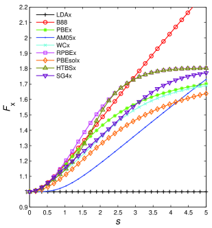
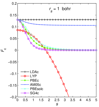
Figure 1: GGA enhancement factors $F_{\text{x}}$ (upper panel) and $F_{\text{c}}$ (lower panel, for $r_{s}=1$ bohr) plotted as a function of $s$.

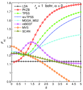
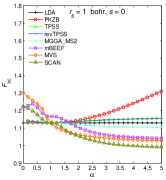
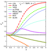
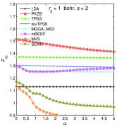
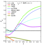
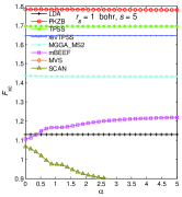
Figure 2: MGGA enhancement factors $F_{\text{xc}}$ plotted as a function of $s$ for three values of $\alpha$ (left panels) and as a function of $\alpha$ for three values of $s$ (right panels). $r_{s}$ is kept fixed to 1 bohr. The $F_{\text{xc}}$ for LDA is also shown.

Figures 1 and 2 show the enhancement factor of most GGA and MGGA functionals tested in this work. Now, we summarize the trends in the performances of GGA functionals and how their are related to the shape of $F_{\text{xc}}$ (mainly determined by the dominating exchange part $F_{\text{x}}$, see upper panel of Fig. 1). LDA, which has the weakest enhancement factor underestimates the equilibrium lattice constant $a_{0}$ of solids. Since large unit cells contain more density gradient (i.e., larger $s$) than small unit cells, then a stronger $F_{\text{xc}}$ (any GGA, see Fig. 1) will lower the total energy more for large unit cells than for smaller ones (a stronger $F_{\text{xc}}$ makes the total energy more negative), and therefore reduce the underestimation of $a_{0}$ obtained with LDA. A good balance is obtained with weak GGAs like AM05 or PBEsol (see Fig. 1) that are among the most accurate for lattice constants. Concerning the cohesive energy $E_{\text{coh}}$ of solids, LDA overestimates the values. Since an isolated atom contains much more density gradient than the solid, then a GGA (w.r.t. LDA) lowers the total energy of the atom by a larger amount than for the solid, thus reducing the overestimation of $E_{\text{coh}}$. In this respect, functionals with a medium $F_{\text{xc}}$ like PBE do a pretty good job. GGAs with a strong $F_{\text{xc}}$ like B88 or RPBE overcorrect LDA and lead to overestimation and underestimation of $a_{0}$ and $E_{\text{coh}}$, respectively. LDA overestimates the atomization energies of molecules as well, and, using the same argument as for $E_{\text{coh}}$, a GGA lowers (w.r.t. LDA) the total energy more for the atoms than for the molecule. However, in this case, functionals with a strong enhancement factor (e.g., B88) are the best performing GGAs, while weaker GGAs reduce only partially the LDA overestimation. One may ask the following question: Why is it necessary to use a $F_{\text{xc}}$ that is stronger for the atomization energy of molecules than for the cohesive energy of solids? The reason is that the degrees of $\rho$-inhomogeneity in the solid and atom (both used to calculate $E_{\text{coh}}$) are very different, such that the appropriate difference (between the solid and atom) in the lowering of the total energy (w.r.t. LDA) is already achieved with a weak $F_{\text{xc}}$. Since the atomization energy of molecules requires calculations on the atoms and molecule, which have more similar inhomogeneities (slightly larger in atoms than in molecule), then a stronger $F_{\text{xc}}$ is required to achieve the desired difference (between the atoms and the molecule) in the lowering of the total energy (w.r.t. LDA).

The above trends hold for GGA functionals that are conventional in the sense that $F_{\text{xc}}$ does not exhibit a strange behavior like oscillations or a suddenly large slope $\partial F_{\text{xc}}/\partial s$ in a small region of $s$. More unconventional forms for $F_{\text{xc}}$ are usually obtained when $F_{\text{xc}}$ contains empirical parameters that are determined by a fit of reference data. The problem of such functionals is a reduced degree of transferability and clear failures in particular cases. An example of such a functional is given by the GGA exchange HTBSHaas et al. (2011) (shown in Fig. 1) that was an attempt to construct a functional which leads to good results for both the lattice constants of solids and atomization energies of molecules: $F_{\text{x}}^{\text{HTBS}}=F_{\text{x}}^{\text{WC}}$ for $s<0.6$ (weak GGA for $s$ values relevant for solids) and $F_{\text{x}}^{\text{HTBS}}=F_{\text{x}}^{\text{RPBE}}$ for $s>2.6$ (strong GGA for $s$ values relevant for finite systems), while a linear combination of WC and RPBE is used for $s\in[0.6,2.6]$. The results were shown to be very good except for systems containing alkali metals whose lattice constants are largely overestimated,Haas et al. (2011) which is due to the large values of $s$ in the core-valence separation region of the alkali metals (see Ref. Haas et al., 2009b).

Concerning the correlation enhancement factor $F_{\text{c}}$ (see lower panel of Fig. 1), we just note that for LYP it behaves differently from the others and that the LDA limit is not recovered, since LYP was designed to reproduce the correlation energy of the helium atom and not of a constant electron density.Lee et al. (1988)

In Fig. 2, the total enhancement factor $F_{\text{xc}}$ of MGGAs is plotted as a function of $s$ for three values of $\alpha$ (on the left panels) and as a function of $\alpha$ for three values of $s$ (on the right panels). The three values of $\alpha$ correspond to regions dominated by a single orbital ($\alpha=0$), of constant electron density ($\alpha=1$), and of overlap of closed shells ($\alpha\gg 5$).Sun et al. (2013a) A few comments can be made. As mentioned above, it can happen for parameterized functionals, like the Minnesota suite of functionals,Zhao and Truhlar (2008b) to have an enhancement factor that shows features like bumps or oscillations that are unphysical and may lead to problems of transferability of the functional. Furthermore, such features lead to numerical noise.Johnson et al. (2009); Mardirossian and Head-Gordon (2015) The mBEEF is such a highly parameterized functional, however, since its parameters were fitted with a regularization procedureWellendorff et al. (2014) the bump visible in Fig. 2 is moderate. A particularity of the SCAN and MVS enhancement factors is to be much more a decreasing function of $s$ and $\alpha$ than the other functionals. Note also the very weak variation of $F_{\text{xc}}$ with respect to $\alpha$ for the TPSS, revTPSS, and MGGA_MS2 functionals. For MGGA functionals, it is maybe more difficult than for GGAs to establish simple relations between the shape of $F_{\text{xc}}$ and the trends in the results. Anyway, it is clear that the additional dependency on the KE density leads to more flexibility and therefore potentially more universal functionals. Finally, we mention Refs. Madsen et al., 2010; Sun et al., 2013a, where it was argued that at small $s$ the enhancement factor should be a decreasing function of $\alpha$ in order to obtain a binding between weakly interacting systems, which is the case for MGGA_MS2, MVS, and SCAN as shown in Fig. 2.

The hybrid functionals can be split into two groups according to the type of HF exchange that is used: the ones that use the unscreened HF exchange and those using only the SR part that was obtained by means of the screened Yukawa potential (details of the implementation can be found in Ref. Tran and Blaha, 2011). The screened hybrid functionals in Table 2 are those whose name starts with YS (Yukawa screened), and among them, YSPBE0Tran and Blaha (2011) is based on the popular functional of Heyd et al.Heyd et al. (2003); Krukau et al. (2006) HSE06 and differs from it by the screening (Yukawa in YSPBE0 versus error function in HSE06) and the way the screening is applied in the semilocal exchange (via the exchange holeHeyd et al. (2003) or via the GGA enhancement factorIikura et al. (2001)). As noticed in Ref. Shimazaki and Asai, 2008, the error function- and Yukawa-screened potentials are very similar if the screening parameter in the Yukawa potential is $3/2$ larger than in the error function. In Ref. Tran and Blaha, 2011 it was shown that HSE06 and YSPBE0 lead to basically the same band gaps, while non-negligible differences were observed for the lattice constants. A comparison between the YSPBE0 results obtained in the present work and the HSE06 results reported in Ref. Schimka et al., 2011 shows that the YSPBE0 lattice constants are in most cases slightly larger by 0.01-0.02 Å, while the atomization energies can differ by 0.05-0.2 eV/atom. Similarly, YSPBEsol0 uses the same underlying semilocal functional (PBEsolPerdew et al. (2009)) and fraction of HF exchange (0.25) as HSEsol (Ref. Schimka et al., 2011). For all screened hybrid functionals tested in this work, a screening parameter $\lambda=0.165$ bohr^-1 was used, which is $3/2$ of the value used in HSE06 with the error function.Krukau et al. (2006) The fraction $\alpha_{\text{x}}$ of HF exchange (indicated in Table 2) varies between 0.09 (MGGA_MS2h) and 0.25 (e.g., PBE0). Among the unscreened hybrid functionals in Table 2, the two most well-known are B3LYPBecke (1993); Stephens et al. (1994) and PBE0.Ernzerhof and Scuseria (1999); Adamo and Barone (1999) Note that in Refs. Tran et al., 2012; Jang and Yu, 2012; Gao et al., , the use of hybrid functionals for metals has been severely criticized, since qualitatively wrong results (e.g., incorrect prediction for the ground state or largely overestimated magnetic moment) were obtained for simple transition metals like Fe or Pd.

The two variants of atom-pairwise dispersion correction [Eq. (4)] that are considered were proposed by Grimme and co-workers.Grimme et al. (2010, 2011) The two schemes, which use the position of atoms to calculate the dispersion coefficients $C_{n}^{AB}$, differ in the damping function $f_{n}^{\text{damp}}$. In the first scheme (DFT-D3, Ref. Grimme et al., 2010), the dispersion energy $E_{\text{c,disp}}^{\text{PW}}$ goes to zero when $R_{AB}\rightarrow 0$, while with the Becke-Johnson (BJ) damping functionJohnson and Becke (2006) that is used in DFT-D3(BJ),Grimme et al. (2011) $E_{\text{c,disp}}^{\text{PW}}$ goes to a nonzero value, which is theoretically correct.Koide (1976) All DFT-D3/D3(BJ) calculations were done with and without the three-body non-additive dispersion term,Grimme et al. (2010) which has little influence on the results for the strongly bound and rare-gas solids. For the layered compounds, however, the effect is larger since adding the three-body term increases the equilibrium lattice constant $c_{0}$ by $\sim 0.1$ Å and decreases the interlayer binding energy by $\sim 10$ meV/atom, which for the latter quantity leads to better agreement with the references results in most cases. In the following, only the results including the three-body term will be shown. Note that in the case of YSPBE0-D3/D3(BJ), the parameters of the D3/D3(BJ) corrections are those that were proposed for the HSE06 functional. The DFT-D3/D3(BJ) dispersion energies were evaluated by using the package provided by GrimmeDFT that supports periodic boundary conditions. Moellmann et al. (2012); Moellmann and Grimme (2014)

IV Results and discussion

IV.1 Strongly bound solids

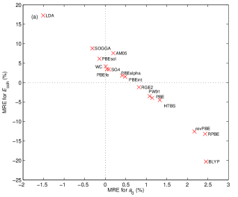
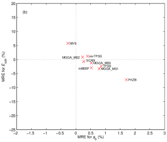
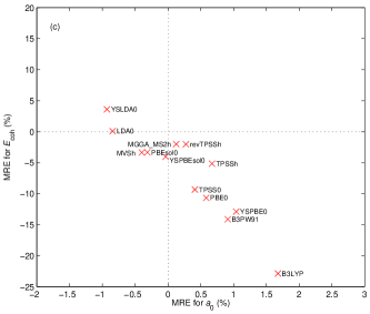
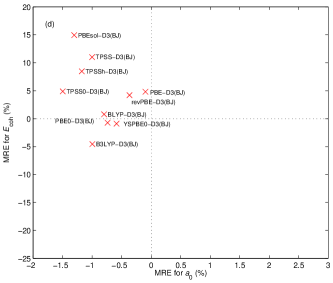
Figure 3: MRE of $a_{0}$ versus MRE of $E_{\text{coh}}$ for the (a) LDA and GGA, (b) MGGA, (c) hybrid, and (d) DFT-D3(BJ) functionals.

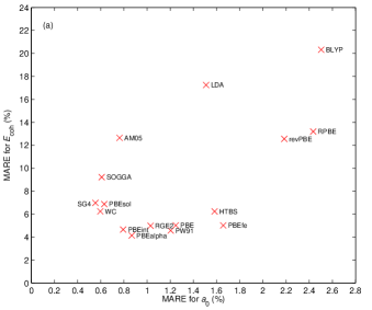
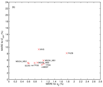
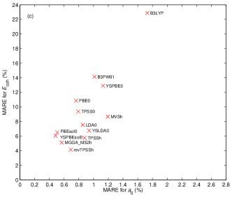
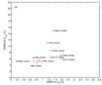
Figure 4: MARE of $a_{0}$ versus MARE of $E_{\text{coh}}$ for the (a) LDA and GGA, (b) MGGA, (c) hybrid, and (d) DFT-D3(BJ) functionals.

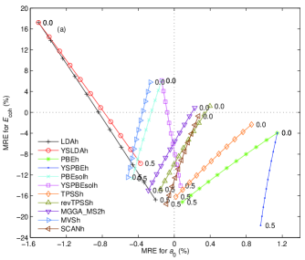
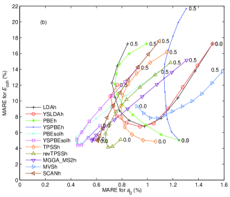
Figure 5: (a) MRE of $a_{0}$ versus MRE of $E_{\text{coh}}$ and (b) MARE of $a_{0}$ versus MARE of $E_{\text{coh}}$ for hybrid functionals with the fraction of HF exchange $\alpha_{\text{x}}$ varied between 0 and 0.5 with steps of 0.05. The lines connecting the data points are guide to the eyes.

Table 2 shows the mean error (ME), mean absolute error (MAE), mean relative error (MRE), and mean absolute error (MARE) on the equilibrium lattice constant $a_{0}$, bulk modulus $B_{0}$, and cohesive energy $E_{\text{coh}}$ for the 44 strongly bound solids. Most of the results are also shown graphically in Figs. 3, and 4, which provide a convenient way to compare the performance of the functionals. The values of $a_{0}$, $B_{0}$, and $E_{\text{coh}}$ for all solids and functionals can be found in the supplementary material (SM).SM_ Since the trends in the MRE/MARE are similar as for the ME/MAE, the discussion of the results will be based mainly on the ME and MAE.

We start with the results for the lattice constant and bulk modulus. These two properties are quite often described with the same accuracy by a functional, but with opposite trends (i.e., an underestimation of $a_{0}$ is accompanied by an overestimation of $B_{0}$ or vice-versa), as seen in Figs. S1-S62 of the SM where the curves for the relative error for $a_{0}$ (left panel) and $B_{0}$ (middle panel) are approximately like mirror images. The smallest MAE for $a_{0}$, 0.021 Å, is obtained by the hybrid-GGA functionals YSPBEsol0 and PBEsol0, which is in line with the conclusion of Ref. Schimka et al., 2011 that combining PBEsol with 25% of HF exchange improves over PBEsol (one of the most accurate GGA functionals for this quantity), PBE, and HSE06 ($\approx$YSPBE0). YSPBEsol0 performs rather well also for $B_{0}$ with a MAE of 8.7 GPa, but is not the best method since a couple of other functionals lead to a MAE around 7.5 GPa, like for example WC, MGGA_MS2, SCAN, PBE0, and PBE-D3(BJ). Note that four functionals (PBEsol, MGGA_MS2, SCAN, and YSPBEsol0) lead to a MARE for $B_{0}$ below 7%. The functionals which perform very well for both $a_{0}$ (MAE not larger than $\sim 0.03$ Å) and $B_{0}$ (MAE below 9 GPa) are the GGAs WC, SOGGA, PBEsol, and SG4, the MGGAs MGGA_MS2 and SCAN, and the hybrids YSPBEsol0 and MGGA_MS2h.

Turning now to the results for the cohesive energy $E_{\text{coh}}$, we can see that the MAE is below $\sim 0.2$ eV/atom for a dozen of functionals, e.g., the GGAs PW91, PBE, and PBEalpha, the MGGA SCAN, the hybrid-MGGA revTPSSh, and a few DFT-D3/D3(BJ) methods. The MAE obtained with YSPBEsol0 and PBEsol0 (the best for the lattice constant) are slightly larger ($\sim 0.27$ eV/atom).

Overall, by considering the results for the three properties ($a_{0}$, $B_{0}$, and $E_{\text{coh}}$), the recent MGGAs MGGA_MS2 and SCAN seem to be the most accurate functionals. They are among the very best functionals for $B_{0}$ and $E_{\text{coh}}$, and only YSPBEsol0, PBEsol0, and SG4 are more accurate for $a_{0}$. Other functionals which are also consistently good for the three properties are the GGAs WC, PBEsol, PBEalpha, PBEint, and SG4, the hybrids YSPBEsol0, MGGA_MS2h, and revTPSSh, and the dispersion-corrected PBE-D3 and PBE-D3(BJ).

It does not seem to be always necessary to use a functional with an atom-pairwise dispersion term [D3 or D3(BJ)] for the strongly bound solids. Actually, adding a dispersion term does not systematically improve the results (we remind that adding a dispersion term should, in principle, shorten bond lengths since the London dispersion interactions are attractive). This is for instance the case with TPSS, TPSSh, and TPSS0, for which the addition of D3(BJ) strongly overcorrects the overestimation of $a_{0}$, leading to large negative ME (and large positive ME for $B_{0}$). In the case of PBEsol (very small ME for $a_{0}$ and $B_{0}$), adding D3 or D3(BJ) can only deteriorate the results since this functional alone does not overestimate the lattice constant on average. However, a clear improvement is obtained with PBE, revPBE, and BLYP. We note that none of these dispersion-corrected methods lead, for instance, to MAE below 0.040 Å for $a_{0}$ and 8 GPa for $B_{0}$ at the same time. Furthermore, the MAE for $B_{0}$ is rather large (above 10 GPa) for many of the dispersion corrected functionals, including PBE0-D3, which leads to a large MAE of 11.7 GPa despite its MAE for $a_{0}$ is only 0.027 Å.

Regarding the hybrid functionals, it is instructive to look at how the MRE and MARE for $a_{0}$ and $E_{\text{coh}}$ vary as functions of the fraction $\alpha_{\text{x}}$ of HF exchange in Eq. (2). This is shown in Fig. 5 for most screened and unscreened hybrid functionals without D3 term, where $\alpha_{\text{x}}$ is varied between 0 and 0.5 with steps of 0.05. The trends observed in Fig. 5(a) for the MRE show two different behaviors. For the LDA-based and YSPBEsolh functionals, the value of the MRE for $a_{0}$ goes in the direction of the positive values when $\alpha_{\text{x}}$ is increased, while the opposite is observed with the other functionals. Interestingly, in most cases except PBEsolh and MVSh, adding a fraction of HF exchange reduces the magnitude of the MRE with respect to the case $\alpha_{\text{x}}=0$. For the MARE [Fig. 5(b)] the main observations are the following: the smallest MARE for $a_{0}$ and $E_{\text{coh}}$ are obtained simultaneously with more or less the same value of $\alpha_{\text{x}}$ in the case of PBEsolh, YSPBEsolh, revTPSSh, MGGA_MS2h, and SCANh. This optimal $\alpha_{\text{x}}$ is $\sim 0$ for MGGA_MS2h and SCANh and $\sim 0.15$ for the others. For MGGA_MS2h and SCANh, it can be argued that since MGGA functionals are more nonlocal than LDA/GGA (in the sense that the KE density $t$ is probably a truly nonlocal functional of $\rho$), then less HF exchange is required when combined with a MGGA. For all other functionals except MVSh, the optimal $\alpha_{\text{x}}$ is larger for $a_{0}$ than for $E_{\text{coh}}$. The exception observed with MVSh should be related to the behavior of its enhancement factor $F_{\text{xc}}$, which has by far the most negative slope as function of $s$ and $\alpha$, as noticed above in Fig. 2.

A few words about the functionals that were not considered in this work should also be added, and in particular about the so-called nonlocal van der Waals (vdW) functionals,Dion et al. (2004) which include a term of the form given by Eq. (5). The first of these functionals which were shown to be, at least, as accurate as PBE for strongly bound solids, namely optPBE-vdW, optB88-vdW, and optB86b-vdW, were proposed in Refs. Klimeš et al., 2010, 2011. In Refs. Klimeš et al., 2011; Schimka et al., 2013; Shulenburger and Mattsson, 2013; Park et al., 2015 it was shown that compared to PBE, optB88-vdW and optPBE-vdW are slightly better for the cohesive energy, while optB86b-vdW is slightly better for the lattice constant. In order to make the SCAN functional more accurate for the treatment of weak interactions, Peng et al.Peng et al. proposed to add a refitted version of the nonlocal vdW functional rVV10.Vydrov and Van Voorhis (2010); Sabatini et al. (2013) For a test set of 50 solids, SCAN+rVV10 was shown to perform similarly as SCAN for the lattice constant, but to increase by about 1% the MARE for the cohesive energy.

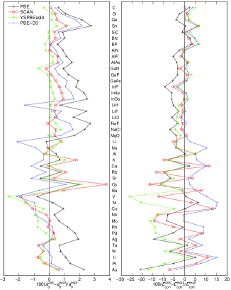
Figure 6: Relative error (in %) in the calculated lattice constant (left panel) and cohesive energy (right panel) for the 44 strongly bound solids.

The detailed results for every solid and functional are shown in the SM,SM_ and Fig. 6 gathers the results for some of the most accurate functionals compared to the standard PBE. In order to avoid a lengthy discussion, only the most interesting observations are now discussed. By looking at Figs. S1-S62, which show the MRE (in %) for the lattice constant, bulk modulus, and cohesive energy, we can immediately see that for many functionals, some of the largest MRE for $a_{0}$ and $B_{0}$ are found for alkali metals (K, Rb, and Cs), alkali-earth metals (Ca, Sr, and Ba), and the transition metal V. For these solids, the MRE for $a_{0}$ increases with the nuclear charge and can reach 4%-8% for Cs. Such large MRE for $a_{0}$ are negative for LDA (accompanied by an overbinding) and positive (underbinding) for several GGAs like revPBE or HTBS and, quite interestingly, all (hybrid)-MGGAs. Such very large overestimations for the heavy alkali metals with TPSS and revTPSS were already reported. Csonka et al. (2009); Perdew et al. (2009); Tao et al. (2010); Schimka et al. (2013) As argued in Ref. Tao et al., 2010, the alkali metals are very soft ($B_{0}$ is below 5 GPa) and have a large polarizable core, such that the long-range core-core dispersion interactions, missing in non-dispersion corrected functionals, should have a non-negligible effect on the results. Therefore, it is maybe for the right reason that a semilocal/hybrid functional, in particular if it is constructed from first-priciples, underbinds the alkali metals. Adding a D3/D3(BJ) term reduces the error for the alkali metals, but overcorrects strongly in some cases [e.g., BLYP-D3(BJ) in Fig. S47]. The results with the DFT-D3/D3(BJ) methods could easily be improved by tuning the coefficients $C_{n}^{AB}$ in Eq. (4). In the case of PBE-D3, for instance, it would be possible to strongly reduce the errors involving the Li atoms by using smaller value for the coefficients, while for all systems with the diamond or zincblende structures, larger coefficients would be required. Such underbinding with the semilocal/hybrid functionals is not observed in the case of the similar alkali-earth metals, which should be due to the following reasons: they are slightly less van der Waals like ($B_{0}$ is above 10 GPa) and the additional valence $s$-electron should reduce the inhomogeneity in $\rho$, making the semilocal functionals more appropriate. The ionic solids Li$X$ and Na$X$ are systems for which the MRE can also very large.

Looking at the trends for the $3d$, $4d$, and $5d$ transition metals, most functionals show the same behavior for the lattice constant; from left to right within a row (e.g., from Nb to Ag), the MRE goes in the direction of the positive values.Ropo et al. (2008); Schimka et al. (2013); Janthon et al. (2014) This behavior is the most pronounced for the strong GGAs like revPBE or BLYP [also if D3/D3(BJ) is included], while it can be strongly reduced with some of the MGGA and hybrid functionals, similarly as RPA does.Schimka et al. (2013)

A summary of this section on the strongly bound solids is the following. Among the tested functionals, about 12 of them are in the group of the best performing for all three properties ($a_{0}$, $B_{0}$, and $E_{\text{coh}}$) at the same time. This includes GGAs (WC, PBEsol, PBEalpha, PBEint, and SG4), MGGAs (MGGA_MS2 and SCAN), hybrids (YSPBEsol0, MGGA_MS2h, and revTPSSh), and dispersion-corrected methods [PBE-D3/D3(BJ)]. Therefore, as also shown more clearly in Figs. 3 and 4, for every type of approximations except LDA, there are a few functionals belonging to the group of the best ones. Furthermore, we have also noticed that MGGA_MS2 and SCAN give the best results when they are not mixed with HF exchange, which is a very interesting property from the practical point of view since the calculation of the HF exchange is very expensive for solids.

IV.2 Weakly bound solids

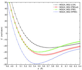
Figure 7: MGGA_MS2 total energy of Ar plotted as a function of the lattice constant $a$. The MGGA_MS2 total-energy functional was evaluated with orbitals/densities generated from various potentials (indicated in parenthesis). The zero of the energy axis was chosen such that the cohesive energy of Ar is given by the value at the minimum of a curve. The reference CCSD(T) values for $a_{0}$ and $E_{\text{coh}}$ are 5.25 Å and 88 meV/atom, respectively.

Table 3: Equilibrium lattice constant $a_{0}$ (in Å) and cohesive energy $E_{\text{coh}}$ (in meV/atom and with opposite sign) of rare-gas solids calculated from various functionals and compared to reference [CCSD(T), very close to experiment] as well as other methods. The results for the LDA, GGA, and GGA+D functionals were obtained from self-consistent calculations, while the PBE orbitals/density were used for the other functionals. Within each group, the functionals are ordered by increasing overall error. For hybrid functionals, the fraction $\alpha_{\text{x}}$ of HF exchange is indicated in parenthesis.

	Ne		Ar		Kr
Functional	$a_{0}$	$E_{\text{coh}}$	$a_{0}$	$E_{\text{coh}}$	$a_{0}$	$E_{\text{coh}}$
LDA
LDA Perdew and Wang (1992)	3.86 (-10%)	87 (234%)	4.94 (-6%)	138 (57%)	5.33 (-5%)	169 (39%)
GGA
PBEalpha Madsen (2007)	4.39 (2%)	23 (-10%)	5.59 (6%)	33 (-62%)	5.97 (7%)	43 (-65%)
SOGGA Zhao and Truhlar (2008a)	4.52 (5%)	23 (-11%)	5.77 (10%)	29 (-67%)	6.14 (10%)	35 (-71%)
RPBE Hammer et al. (1999)	4.74 (10%)	26 (0%)	6.25 (19%)	28 (-68%)	6.83 (22%)	29 (-76%)
PBE Perdew et al. (1996a)	4.60 (7%)	19 (-26%)	5.96 (13%)	23 (-73%)	6.42 (15%)	27 (-78%)
HTBS Haas et al. (2011)	4.80 (12%)	23 (-12%)	6.34 (21%)	25 (-72%)	6.93 (24%)	26 (-79%)
PW91 Perdew et al. (1992)	4.62 (7%)	47 (82%)	6.05 (15%)	49 (-44%)	6.55 (17%)	51 (-58%)
PBEsol Perdew et al. (2008)	4.70 (9%)	12 (-54%)	5.88 (12%)	17 (-81%)	6.13 (10%)	23 (-81%)
PBEint Fabiano et al. (2010)	4.78 (11%)	14 (-46%)	6.21 (18%)	17 (-81%)	6.67 (19%)	20 (-84%)
RGE2 Ruzsinszky et al. (2009)	4.92 (14%)	14 (-45%)	6.43 (23%)	16 (-81%)	6.99 (25%)	18 (-85%)
WC Wu and Cohen (2006)	4.87 (13%)	12 (-54%)	6.34 (21%)	14 (-84%)	6.86 (23%)	16 (-87%)
PBEfe Sarmiento-Pérez et al. (2015)	3.88 (-10%)	99 (280%)	5.00 (-5%)	152 (73%)	5.42 (-3%)	184 (51%)
SG4 Constantin et al. (2016)	5.25 (22%)	9 (-67%)	$>$ 6.6 ($>$ 26%)		$>$ 7.1 ($>$ 27%)
revPBE Zhang and Yang (1998)	5.31 (24%)	7 (-74%)	$>$ 6.6 ($>$ 26%)		$>$ 7.1 ($>$ 27%)
BLYP Becke (1988); Lee et al. (1988)	$>$ 5.6 ($>$ 31%)		$>$ 6.6 ($>$ 26%)		$>$ 7.1 ($>$ 27%)
AM05 Armiento and Mattsson (2005)	$>$ 5.6 ($>$ 31%)		$>$ 6.6 ($>$ 26%)		$>$ 7.1 ($>$ 27%)
MGGA
MGGA_MS2 Sun et al. (2013b)	4.31 (0%)	26 (1%)	5.48 (4%)	30 (-66%)	5.96 (6%)	45 (-63%)
MGGA_MS1 Sun et al. (2013b)	4.34 (1%)	26 (0%)	5.58 (6%)	27 (-69%)	6.10 (9%)	40 (-67%)
MGGA_MS0 Sun et al. (2012)	4.16 (-3%)	40 (53%)	5.41 (3%)	46 (-47%)	5.89 (5%)	61 (-50%)
SCAN Sun et al. (2015a)	4.03 (-6%)	54 (107%)	5.31 (1%)	61 (-30%)	5.74 (2%)	72 (-41%)
PKZB Perdew et al. (1999)	4.66 (9%)	27 (2%)	6.20 (18%)	26 (-70%)	6.76 (21%)	30 (-75%)
MVS Sun et al. (2015b)	4.02 (-6%)	59 (125%)	5.41 (3%)	56 (-37%)	5.79 (3%)	69 (-43%)
TPSS Tao et al. (2003)	4.92 (15%)	11 (-59%)	6.45 (23%)	11 (-87%)	6.98 (25%)	15 (-88%)
mBEEF Wellendorff et al. (2014)	3.92 (-9%)	134 (416%)	5.26 (0%)	142 (62%)	5.75 (3%)	161 (32%)
revTPSS Perdew et al. (2009)	5.05 (17%)	7 (-72%)	$>$ 6.6 ($>$ 26%)		7.04 (26%)	12 (-90%)
hybrid-LDA
LDA0 Perdew and Wang (1992); Perdew et al. (1996b) (0.25)	4.00 (-7%)	51 (96%)	5.18 (-1%)	71 (-19%)	5.57 (0%)	90 (-26%)
YSLDA0 Perdew and Wang (1992); Perdew et al. (1996b) (0.25)	3.96 (-8%)	60 (131%)	5.12 (-2%)	86 (-2%)	5.51 (-1%)	108 (-11%)
hybrid-GGA
PBE0 Ernzerhof and Scuseria (1999); Adamo and Barone (1999) (0.25)	4.61 (7%)	11 (-57%)	5.96 (14%)	15 (-83%)	6.41 (15%)	19 (-84%)
PBEsol0 Perdew et al. (2008, 1996b) (0.25)	4.66 (8%)	7 (-75%)	5.79 (10%)	12 (-86%)	6.06 (8%)	20 (-84%)
YSPBE0 Krukau et al. (2006); Tran and Blaha (2011) (0.25)	4.76 (11%)	10 (-60%)	6.21 (18%)	14 (-84%)	6.69 (19%)	17 (-86%)
YSPBEsol0 Schimka et al. (2011) (0.25)	4.93 (15%)	5 (-81%)	6.26 (19%)	8 (-91%)	6.55 (17%)	11 (-91%)
B3LYP Stephens et al. (1994) (0.20)	$>$ 5.6 ($>$ 31%)		$>$ 6.6 ($>$ 26%)		$>$ 7.1 ($>$ 27%)
B3PW91 Becke (1993) (0.20)	$>$ 5.6 ($>$ 31%)		$>$ 6.6 ($>$ 26%)		$>$ 7.1 ($>$ 27%)
hybrid-MGGA
MGGA_MS2h Sun et al. (2013b) (0.09)	4.31 (0%)	23 (-11%)	5.48 (4%)	27 (-70%)	5.97 (7%)	41 (-67%)
MVSh Sun et al. (2015b) (0.25)	4.05 (-6%)	40 (55%)	5.44 (4%)	40 (-55%)	5.83 (4%)	52 (-58%)
TPSSh Staroverov et al. (2003) (0.10)	4.93 (15%)	8 (-67%)	6.46 (23%)	9 (-90%)	6.98 (25%)	13 (-90%)
TPSS0 Tao et al. (2003); Perdew et al. (1996b) (0.25)	4.96 (15%)	5 (-80%)	6.47 (23%)	6 (-93%)	6.98 (25%)	9 (-92%)
revTPSSh Csonka et al. (2010) (0.10)	5.06 (18%)	5 (-79%)	$>$ 6.6 ($>$ 26%)		7.03 (26%)	10 (-92%)
GGA+D
revPBE-D3(BJ) Grimme et al. (2011)	4.80 (12%)	25 (-2%)	5.67 (8%)	82 (-7%)	5.96 (7%)	126 (3%)
PBEsol-D3(BJ) Goerigk and Grimme (2011)	4.59 (7%)	22 (-16%)	5.46 (4%)	71 (-19%)	5.69 (2%)	116 (-5%)
revPBE-D3 Grimme et al. (2010)	4.73 (10%)	25 (-4%)	5.64 (7%)	68 (-23%)	5.85 (5%)	109 (-11%)
PBE-D3(BJ) Grimme et al. (2011)	4.46 (4%)	37 (42%)	5.49 (5%)	86 (-2%)	5.85 (5%)	117 (-4%)
PBEsol-D3 Goerigk and Grimme (2011)	4.53 (5%)	29 (13%)	5.37 (2%)	61 (-31%)	5.58 (0%)	102 (-17%)
BLYP-D3 Grimme et al. (2010)	4.25 (-1%)	16 (-38%)	5.35 (2%)	70 (-21%)	5.70 (2%)	127 (4%)
PBE-D3 Grimme et al. (2010)	4.39 (2%)	46 (78%)	5.58 (6%)	83 (-6%)	5.90 (5%)	113 (-8%)
BLYP-D3(BJ) Grimme et al. (2011)	4.58 (7%)	3 (-89%)	5.37 (2%)	71 (-19%)	5.67 (1%)	134 (10%)
RPBE-D3 DFT	4.49 (4%)	52 (101%)	5.66 (8%)	91 (3%)	6.03 (8%)	116 (-5%)
MGGA+D
TPSS-D3(BJ) Grimme et al. (2011)	4.69 (9%)	28 (7%)	5.67 (8%)	78 (-11%)	5.97 (7%)	118 (-3%)
TPSS-D3 Grimme et al. (2010)	4.53 (6%)	36 (39%)	5.69 (8%)	76 (-14%)	5.99 (7%)	111 (-9%)
MGGA_MS2-D3 Sun et al. (2013b)	4.19 (-3%)	55 (113%)	5.43 (3%)	83 (-6%)	5.91 (5%)	105 (-14%)
MGGA_MS1-D3 Sun et al. (2013b)	4.14 (-4%)	60 (132%)	5.37 (2%)	96 (9%)	5.83 (4%)	121 (-1%)
MGGA_MS0-D3 Sun et al. (2013b)	4.10 (-5%)	70 (170%)	5.38 (2%)	98 (11%)	5.85 (4%)	120 (-2%)
hybrid-GGA+D
PBE0-D3(BJ) Grimme et al. (2011) (0.25)	4.45 (4%)	28 (7%)	5.46 (4%)	82 (-7%)	5.79 (3%)	121 (-1%)
B3LYP-D3 Grimme et al. (2010) (0.20)	4.25 (-1%)	23 (-10%)	5.30 (1%)	68 (-23%)	5.61 (0%)	129 (5%)
YSPBE0-D3(BJ) DFT (0.25)	4.62 (8%)	23 (-11%)	5.66 (8%)	75 (-15%)	5.98 (7%)	116 (-5%)
PBE0-D3 Grimme et al. (2010) (0.25)	4.39 (2%)	36 (40%)	5.45 (4%)	74 (-16%)	5.71 (2%)	114 (-6%)
B3LYP-D3(BJ) Grimme et al. (2011) (0.20)	4.39 (2%)	12 (-52%)	5.32 (1%)	78 (-12%)	5.65 (1%)	135 (11%)
YSPBE0-D3 DFT (0.25)	4.46 (4%)	33 (25%)	5.75 (9%)	60 (-32%)	6.21 (11%)	74 (-39%)
hybrid-MGGA+D
TPSSh-D3(BJ) Hoffmann et al. (2014) (0.10)	4.69 (9%)	25 (-3%)	5.65 (8%)	79 (-10%)	5.94 (6%)	122 (0%)
TPSS0-D3 Grimme et al. (2010) (0.25)	4.53 (5%)	29 (13%)	5.64 (7%)	66 (-25%)	5.78 (3%)	108 (-12%)
TPSS0-D3(BJ) Grimme et al. (2011) (0.25)	4.66 (8%)	21 (-18%)	5.57 (6%)	70 (-21%)	5.81 (4%)	112 (-8%)
TPSSh-D3 Goerigk and Grimme (2011) (0.10)	4.55 (6%)	33 (28%)	5.70 (9%)	70 (-20%)	5.91 (6%)	108 (-12%)
MGGA_MS2h-D3 Sun et al. (2013b) (0.09)	4.18 (-3%)	52 (100%)	5.44 (4%)	79 (-10%)	5.91 (5%)	101 (-17%)
Previous works
optB88-vdW Klimeš et al. (2010) (Ref. Tran and Hutter, 2013)	4.24 (-1%)	59 (127%)	5.24 (0%)	143 (62%)	5.63 (1%)	181 (48%)
C09x-vdW Cooper (2010) (Ref. Tran and Hutter, 2013)	4.50 (5%)	62 (138%)	5.33 (2%)	128 (45%)	5.64 (1%)	163 (34%)
rVV10 Vydrov and Van Voorhis (2010); Sabatini et al. (2013) (Ref. Tran and Hutter, 2013)	4.19 (-2%)	49 (88%)	5.17 (-2%)	117 (33%)	5.53 (-1%)	162 (33%)
rev-vdW-DF2 Hamada (2014) (Ref. Callsen and Hamada, 2015)	4.43 (3%)	30 (15%)	5.35 (2%)	90 (2%)	5.71 (2%)	120 (-2%)
PBE+TS Tkatchenko and Scheffler (2009) (Ref. Al-Saidi et al., 2012)	4.42 (3%)	43 (65%)	5.51 (5%)	83 (-6%)	5.90 (5%)	97 (-20%)
RPA (Ref. Harl and Kresse, 2008)	4.5 (5%)	17 (-35%)	5.3 (1%)	83 (-6%)	5.7 (2%)	112 (-8%)
Expt. (Ref. Rościszewski et al., 2000)	4.29	26	5.25	88	5.63	122
CCSD(T) (Ref. Rościszewski et al., 2000)	4.30	26	5.25	88	5.60	122

Table 4: Equilibrium lattice constant $c_{0}$ (in Å) and interlayer binding energy $E_{\text{b}}$ (in meV/atom and with opposite sign) of layered solids calculated from various functionals and compared to reference (RPA) as well as other methods. The results for the LDA, GGA, and GGA+D functionals were obtained from self-consistent calculations, while the PBE orbitals/density were used for the other functionals. Within each group, the functionals are ordered by increasing overall error. For hybrid functionals, the fraction $\alpha_{\text{x}}$ of HF exchange is indicated in parenthesis.

	Graphite		h-BN
Functional	$c_{0}$	$E_{\text{b}}$	$c_{0}$	$E_{\text{b}}$
LDA
LDA Perdew and Wang (1992)	6.7 (0%)	24 (-50%)	6.5 (-3%)	28 (-28%)
GGA
PBEfe Sarmiento-Pérez et al. (2015)	7.0 (5%)	21 (-57%)	6.9 (3%)	24 (-39%)
SOGGA Zhao and Truhlar (2008a)	7.3 (9%)	4 (-91%)	7.0 (5%)	7 (-83%)
PBEsol Perdew et al. (2008)	7.3 (9%)	4 (-92%)	7.0 (6%)	6 (-84%)
PBEalpha Madsen (2007)	7.6 (14%)	4 (-91%)	7.3 (10%)	6 (-84%)
PBE Perdew et al. (1996a)	$\sim 8.8$ (31%)	1 (-97%)	$\sim 8.5$ (28%)	2 (-94%)
PW91 Perdew et al. (1992)	$\sim 9.3$ (38%)	2 (-95%)	$\sim 9.0$ (36%)	3 (-93%)
PBEint Fabiano et al. (2010)	$\sim 9.3$ (39%)	1 (-98%)	$\sim 9.0$ (35%)	2 (-96%)
WC Wu and Cohen (2006)	$\sim 9.7$ (45%)	1 (-99%)	$\sim 9.5$ (42%)	1 (-97%)
RPBE Hammer et al. (1999)	$\sim 9.8$ (46%)	1 (-97%)	$\sim 9.8$ (47%)	2 (-96%)
HTBS Haas et al. (2011)	$\sim 9.9$ (48%)	1 (-98%)	$\sim 9.9$ (49%)	2 (-96%)
RGE2 Ruzsinszky et al. (2009)	$\sim 10.0$ (49%)	1 (-99%)	$\sim 10.0$ (49%)	1 (-97%)
SG4 Constantin et al. (2016)	$\sim 11.0$ (64%)	0 (-99%)	$\sim 11.0$ (65%)	1 (-98%)
revPBE Zhang and Yang (1998)	$\sim 11.3$ (69%)	0 (-99%)	$\sim 11.3$ (70%)	1 (-98%)
AM05 Armiento and Mattsson (2005)	$>$ 19 ($>$ 176%)		$>$ 19 ($>$ 188%)
BLYP Becke (1988); Lee et al. (1988)	$>$ 19 ($>$ 176%)		$>$ 19 ($>$ 188%)
MGGA
MVS Sun et al. (2015b)	6.6 (-1%)	32 (-34%)	6.4 (-4%)	38 (-4%)
SCAN Sun et al. (2015a)	6.9 (3%)	20 (-59%)	6.8 (2%)	21 (-46%)
mBEEF Wellendorff et al. (2014)	7.8 (16%)	13 (-72%)	7.7 (16%)	14 (-63%)
MGGA_MS2 Sun et al. (2013b)	7.2 (7%)	8 (-83%)	7.0 (5%)	10 (-74%)
MGGA_MS0 Sun et al. (2012)	7.4 (11%)	8 (-83%)	7.3 (9%)	9 (-76%)
MGGA_MS1 Sun et al. (2013b)	7.8 (16%)	5 (-90%)	7.7 (16%)	6 (-86%)
PKZB Perdew et al. (1999)	7.9 (19%)	4 (-91%)	7.9 (18%)	5 (-88%)
revTPSS Perdew et al. (2009)	$>$ 19 ($>$ 176%)		$\sim 9.8$ (47%)	1 (-98%)
TPSS Tao et al. (2003)	$>$ 19 ($>$ 176%)		$\sim 9.9$ (49%)	1 (-98%)
hybrid-LDA
YSLDA0 Perdew and Wang (1992); Perdew et al. (1996b) (0.25)	7.0 (4%)	15 (-70%)	6.7 (1%)	18 (-53%)
LDA0 Perdew and Wang (1992); Perdew et al. (1996b) (0.25)	7.1 (5%)	12 (-74%)	6.8 (2%)	16 (-60%)
hybrid-GGA
PBEsol0 Perdew et al. (2008, 1996b) (0.25)	7.3 (9%)	5 (-90%)	7.0 (5%)	7 (-81%)
YSPBEsol0 Schimka et al. (2011) (0.25)	$\sim 7.8$ (17%)	1 (-97%)	$\sim 7.3$ (10%)	3 (-92%)
PBE0 Ernzerhof and Scuseria (1999); Adamo and Barone (1999) (0.25)	$\sim 8.4$ (25%)	2 (-97%)	$\sim 8.0$ (20%)	3 (-94%)
YSPBE0 Krukau et al. (2006); Tran and Blaha (2011) (0.25)	$\sim 9.3$ (39%)	1 (-98%)	$\sim 9.0$ (36%)	1 (-97%)
B3LYP Stephens et al. (1994) (0.20)	$>$ 19 ($>$ 176%)		$>$ 19 ($>$ 188%)
B3PW91 Becke (1993) (0.20)	$>$ 19 ($>$ 176%)		$>$ 19 ($>$ 188%)
hybrid-MGGA
MVSh Sun et al. (2015b) (0.25)	6.7 (0%)	25 (-48%)	6.5 (-3%)	31 (-22%)
MGGA_MS2h Sun et al. (2013b) (0.09)	7.2 (7%)	8 (-83%)	7.0 (5%)	10 (-74%)
revTPSSh Csonka et al. (2010) (0.10)	$>$ 19 ($>$ 176%)		$\sim 9.4$ (41%)	1 (-98%)
TPSSh Staroverov et al. (2003) (0.10)	$>$ 19 ($>$ 176%)		$\sim 9.8$ (48%)	1 (-98%)
TPSS0 Tao et al. (2003); Perdew et al. (1996b) (0.25)	$>$ 19 ($>$ 176%)		$\sim 9.6$ (44%)	1 (-98%)
GGA+D
RPBE-D3 DFT	6.8 (1%)	39 (-19%)	6.7 (0%)	39 (0%)
PBE-D3(BJ) Grimme et al. (2011)	6.8 (2%)	43 (-10%)	6.7 (0%)	44 (12%)
PBEsol-D3 Goerigk and Grimme (2011)	6.7 (0%)	38 (-20%)	6.6 (-2%)	42 (8%)
PBE-D3 Grimme et al. (2010)	7.1 (5%)	39 (-19%)	6.8 (3%)	41 (5%)
PBEsol-D3(BJ) Goerigk and Grimme (2011)	6.7 (-1%)	52 (8%)	6.5 (-3%)	53 (36%)
revPBE-D3 Grimme et al. (2010)	6.6 (-2%)	53 (10%)	6.5 (-2%)	52 (33%)
BLYP-D3 Grimme et al. (2010)	6.8 (1%)	59 (22%)	6.7 (0%)	58 (49%)
revPBE-D3(BJ) Grimme et al. (2011)	6.5 (-4%)	67 (41%)	6.3 (-5%)	69 (77%)
BLYP-D3(BJ) Grimme et al. (2011)	6.6 (-2%)	70 (46%)	6.5 (-3%)	71 (83%)
MGGA+D
MGGA_MS1-D3 Sun et al. (2013b)	6.9 (2%)	46 (-4%)	6.8 (2%)	44 (12%)
MGGA_MS2-D3 Sun et al. (2013b)	6.8 (2%)	45 (-6%)	6.6 (-1%)	46 (17%)
MGGA_MS0-D3 Sun et al. (2013b)	7.0 (5%)	42 (-13%)	6.8 (3%)	42 (7%)
TPSS-D3 Grimme et al. (2010)	6.7 (0%)	47 (-1%)	6.5 (-2%)	50 (28%)
TPSS-D3(BJ) Grimme et al. (2011)	6.5 (-3%)	58 (21%)	6.3 (-5%)	60 (53%)
hybrid-GGA+D
YSPBE0-D3(BJ) DFT (0.25)	7.0 (4%)	46 (-5%)	6.8 (2%)	46 (19%)
PBE0-D3 Grimme et al. (2010) (0.25)	6.9 (2%)	41 (-14%)	6.7 (0%)	45 (16%)
PBE0-D3(BJ) Grimme et al. (2011) (0.25)	6.7 (0%)	50 (3%)	6.5 (-2%)	51 (31%)
B3LYP-D3 Grimme et al. (2010) (0.20)	6.8 (2%)	50 (5%)	6.7 (1%)	54 (38%)
YSPBE0-D3 DFT (0.25)	7.3 (9%)	30 (-36%)	7.1 (6%)	30 (-23%)
B3LYP-D3(BJ) Grimme et al. (2011) (0.20)	6.7 (-1%)	62 (29%)	6.5 (-3%)	64 (64%)
hybrid-MGGA+D
MGGA_MS2h-D3 Sun et al. (2013b) (0.09)	6.8 (2%)	45 (-7%)	6.6 (-1%)	46 (18%)
TPSSh-D3 Goerigk and Grimme (2011) (0.10)	6.7 (0%)	47 (-2%)	6.5 (-2%)	51 (30%)
TPSS0-D3 Grimme et al. (2010) (0.25)	6.6 (-1%)	48 (0%)	6.5 (-3%)	53 (35%)
TPSS0-D3(BJ) Grimme et al. (2011) (0.25)	6.5 (-3%)	56 (17%)	6.2 (-6%)	60 (54%)
TPSSh-D3(BJ) Hoffmann et al. (2014) (0.10)	6.5 (-3%)	61 (28%)	6.3 (-5%)	63 (62%)
Previous works
optB88-vdW Klimeš et al. (2010) (Ref. Björkman, 2014)	6.76 (1%)	66 (38%)	6.64 (1%)	67 (72%)
C09x-vdW Cooper (2010) (Ref. Björkman, 2014)	6.54 (-2%)	71 (48%)	6.42 (-3%)	73 (87%)
VV10 Vydrov and Van Voorhis (2010); Sabatini et al. (2013) (Ref. Björkman, 2012)	6.68 (0%)	71 (48%)	6.57 (0%)	70 (79%)
rev-vdW-DF2 Hamada (2014) (Ref. Hamada, 2014)	6.64 (-1%)	60 (25%)	6.56 (-1%)	57 (46%)
PW86R-VV10sol Björkman (2012) (Ref. Björkman, 2012)	6.98 (5%)	44 (-8%)	6.87 (4%)	43 (10%)
AM05-VV10sol Björkman (2012) (Ref. Björkman, 2012)	6.99 (5%)	45 (-6%)	6.84 (4%)	41 (5%)
PBE+TS Tkatchenko and Scheffler (2009) (Ref. Bučko et al., 2013)	6.68 (0%)	82 (71%)	6.64 (1%)	87 (123%)
PBE+TS+SCS Tkatchenko et al. (2012) (Ref. Bučko et al., 2013)	6.75 (1%)	55 (15%)	6.67 (1%)	73 (87%)
RPA (Refs. Lebègue et al., 2010; Björkman et al., 2012)	6.68	48	6.60	39

In this section, the results for rare-gas solids (Ne, Ar, and Kr) and layered solids (graphite and h-BN) are discussed. Rare-gas dimers and solids, which are bound by the dispersion interactions, have been commonly used for the testing of theoretical methods (see Refs. Kullie and Saue, 2012; Roy et al., 2012; Tran and Hutter, 2013; Moellmann and Grimme, 2014; Callsen and Hamada, 2015; Patra et al., 2015 for the most recent works). The same is true for graphite and h-BN which are stacks of weakly bound hexagonal layers. Björkman et al. (2012, 2012); Björkman (2012, 2014); Graziano et al. (2012); Hamada (2014); Bučko et al. (2013); Rêgo et al. (2015)

As mentioned in Sec. II, the results for such weakly bound systems are more sensitive to self-consistency effects than for the strongly bound solids. Figure 7 shows the example for Ar, where the MGGA_MS2 total-energy curves were obtained with four different sets of orbitals/density. Actually, this is a particularly bad case where the spread in the values for $a_{0}$ (5.4-5.7 Å) is two orders of magnitude larger than for most strongly bound solids and the spread for $E_{\text{coh}}$ is of the same magnitude as $E_{\text{coh}}$ itself. We observed that in general the spread in $a_{0}$ is larger for functionals which lead to shallow minimum. This shows that there is some non-negligible degree of uncertainty in the results for the MGGA and hybrid functionals of Tables 3 and 4 that were obtained non-self-consistently with PBE orbitals/density instead of self-consistently as it should be. Thus, for these functionals the discussion should be kept at a qualitative level. On the other hand, the main conclusions of this section should not be affect too significantly, since for such weakly bound systems the errors with DFT functionals are often extremely large such that only the trends are usually discussed.

IV.2.1 Rare-gas solids

The results for the lattice constant and cohesive energy of the rare-gas solids are shown in Table 3. The error (indicated in parenthesis) is with respect to accurate results obtained from the CCSD(T) method.Rościszewski et al. (2000) Also shown are results taken from Refs. Al-Saidi et al., 2012; Tran and Hutter, 2013; Callsen and Hamada, 2015; Harl and Kresse, 2008 that were obtained with nonlocal dispersion-corrected functionals [Eq. (5)], the atom-pairwise method of Tkatchenko and Scheffler,Tkatchenko and Scheffler (2009) and post-PBE RPA calculations. In a few cases, no minimum in the total-energy curve was obtained in the range of lattice constants that we have considered (largest values are 5.6, 6.6, 7.1 Å for Ne, Ar, Kr). This concerns the functionals revPBE, AM05, SG4, revTPSS(h), and those using B88 exchange (BLYP, B3LYP, and B3PW91). No minimum at all should exist with the B88-based functionals (see, e.g., Refs. Kristyán and Pulay, 1994; Pérez-Jordá and Becke, 1995; Wu and Yang, 2002; Xu et al., 2005), while only a very weak minimum at a larger lattice constant could eventually be expected with revPBE (see Ref. Tkatchenko and von Lilienfeld, 2008) and revTPSS (see Ref. Sun et al., 2013a). Note that no or a very weak binding is typically obtained by GGA functionals which violate the local Lieb-Oxford boundLieb and Oxford (1981) because of an enhancement factor that is too large at large $s$ ($s\gtrsim 5$) like B88 and AM05 (see Fig. 1). The importance of the behavior of the enhancement factor at large $s$ for noncovalent interactions was underlined in Refs. Wesolowski et al., 1997; Zhang et al., 1997.

Unsurprisingly, the best functionals are those which include the atom-pairwise dispersion term D3/D3(BJ), since for many of them the errors are below $\sim 8$% for $a_{0}$ and below $\sim 20$% for $E_{\text{coh}}$ for all three rare gases. Such results are expected since the atom-dependent parameters in Eq. (4) (computed almost from first principlesGrimme et al. (2010)) should remain always accurate in the case of interaction between rare-gas atoms, whether it is in the dimer or in the solid. Note, however, that the error for the cohesive energy of Ne is above 100% for all MGGA_MS$n$(h)-D3 functionals, which may be due to the fact that only the term $n=6$ in Eq. (4) has been considered for these functionals.Sun et al. (2013b) All other functionals, without exception, lead to errors for $E_{\text{coh}}$ which are above 50% for at least two rare gases. These large errors are always due to an underestimation for Ar and Kr, but not for Ne (overestimation with the MGGAs and underestimation with the others). For MGGA_MS2 and SCAN, the largest errors are $-66$% (Ar) and 107% (Ne), respectively. Note that the GGA PBEfe and MGGA mBEEF overestimate the cohesive energy even more than LDA does. For $a_{0}$, the values obtained with the GGA PBEalpha and all modern (hybrid-)MGGAs like MGGA_MS2, SCAN, and mBEEF are in fair agreement with the CCSD(T) results since the errors are of the same order as with most dispersion-corrected functionals (below 8%).

Concerning previous works reporting tests on other functionals, we mention Ref. Tran and Hutter, 2013 where several variants of the nonlocal van der Waals functionals were tested on rare-gas dimers (from He₂ to Kr₂) and solids (Ne, Ar, and Kr). The conclusion was that rVV10Vydrov and Van Voorhis (2010); Sabatini et al. (2013) leads to excellent results for the dimers and is among the good ones for the solids along with optB88-vdWKlimeš et al. (2010) and C09x-vdW.Cooper (2010) However, with these three nonlocal functionals rather large errors in $E_{\text{coh}}$ were still observed for the solids (results shown in Table 3), such that overall these functionals are less accurate than DFT-D3/D3(BJ) for the rare-gas solids. Another nonlocal functional, rev-vdW-DF2, was recently proposed by Hamada,Hamada (2014) and the results on rare-gas solidsCallsen and Hamada (2015) (see Table 3) are as good as the DFT-D3/D3(BJ) results and, therefore, better than for the other three nonlocal functionals. For the Ar and Kr dimers, the SCAN+rVV10 functional was shown to be as accurate as rVV10,Peng et al. however it has not been tested on rare-gas solids. Finally, we also mention the RPA (fifth rung of Jacob’s ladder) results from Ref. Harl and Kresse, 2008 which are rather accurate overall, as shown in Table 3. Concerning other semilocal approximations not augmented with a dispersion correction, previous works reported unsuccessful attempts to find such a functional leading to accurate results for all rare-gas dimers at the same time (see, e.g., Refs. Xu et al., 2005; Zhao and Truhlar, 2006a).

The summary for the rare-gas solids is the following. For the cohesive energy, the functionals which include an atom-pairwise term D3/D3(BJ) clearly outperform the others. It was also observed that the MGGAs do not improve over the GGAs for $E_{\text{coh}}$. However, for the lattice constant, MGGAs are superior to the GGAs and perform as well as the dispersion corrected-functionals. Among the previous works also considering rare-gas solids in their test set, we noted that the rev-vdW-DF2 nonlocal functional Hamada (2014); Callsen and Hamada (2015) shows similar accuracy as the DFT-D3/D3(BJ) methods.

IV.2.2 Layered solids

Turning now to the layered solids graphite and h-BN, the results for the equilibrium lattice constant $c_{0}$ (the interlayer distance is $c_{0}/2$) and interlayer binding energy $E_{\text{b}}$ are shown in Table 4. Since for these two systems we are interested only in the interlayer properties, the intralayer lattice constant $a$ was kept fixed at the experimental value of 2.462 and 2.503 Å for graphite and h-BN, respectively. As in the recent works of Björkman et al., Björkman et al. (2012, 2012); Björkman (2012, 2014) the results from the RPA method,Lebègue et al. (2010); Björkman et al. (2012) which are in very good agreement with experiment and Monte-Carlo simulationSpanu et al. (2009) for graphite, are used as reference. No experimental result for $E_{\text{b}}$ for h-BN seems to be available.

The results with the GGA functionals are extremely inaccurate since for all these methods, except PBEfe, there is no or a very tiny binding between the layers (underestimation of $E_{\text{b}}$ by more than 90%) and a huge overestimation of $c_{0}$ by at least 0.5 Å. The underestimation of $E_{\text{b}}$ with PBEfe is $\sim 50\%$ and $c_{0}$ is too large by $\sim 0.3$ Å. LDA also underestimates $E_{b}$ by $\sim 40\%$, but leads to interlayer distances which agree quite well with RPA and, actually, perfectly for graphite. The best MGGA functional is MVS, whose relative error is $-34\%$ for the binding energy of graphite, but below 5% otherwise. SCAN performs slightly worse since $E_{\text{b}}$ is too small by $\sim 50\%$ for both graphite and h-BN, while MGGA_MS2 leads to disappointingly small binding energies. The other MGGAs, including mBEEF, lead to very small (large) values for $E_{\text{b}}$ ($c_{0}$). Note that the results obtained with mBEEF show totally different trends as those for the rare gases (large overbinding for the rare gases and large underbinding for graphite and h-BN), which is maybe due to the nonsmooth form of this functional (see Fig. 2) such that the results are more unpredictable. Among the hybrid functionals, MVSh is the only one which leads to somehow reasonable results, with errors for $E_{\text{b}}$ that are slightly larger than for the underlying semilocal MVS. Let us remark that all functionals without dispersion correction underestimate the interlayer binding energy of graphite and h-BN, while it was not the case for the cohesive energy of the rare-gas solids.

Adding the D3 or D3(BJ) dispersion term usually improves the agreement with RPA, such that for many of these methods the magnitude of the relative error is below 20% and 3% for $E_{\text{b}}$ and $c_{0}$, respectively. Such errors can be considered as relatively modest. Among the computationally cheap GGA+D, the accurate functionals are PBE-D3/D3(BJ), RPBE-D3, and PBEsol-D3.

The results obtained with many other methods are available in the literature Björkman et al. (2012, 2012); Björkman (2012, 2014); Graziano et al. (2012); Hamada (2014); Bučko et al. (2013); Rêgo et al. (2015) (see Ref. Rêgo et al., 2015 for a collection of values for graphite), and those obtained from the methods that were already selected for the discussion on the rare gases are shown in Table 4. The nonlocal functionals optB88-vdW, C09x-vdW, VV10, and rev-vdW-DF2 as well as PBE+TS(+SCS) lead to very good agreement with RPA for the interlayer lattice constant (errors in the range 0-2%), however, in most cases there is a non-negligible overbinding above 40%. Also shown in Table 4, are the results obtained with the nonlocal functionals PW86R-VV10 and AM05-VV10sol which contain parameters that were fitted specifically to RPA binding energies of 26 layered solids including graphite and h-BN.Björkman (2012) Unsurprisingly, the errors obtained with PW86R-VV10 and AM05-VV10sol for $E_{\text{b}}$ are very small (below 10%), but the price to pay are errors for $c_{0}$ that are clearly larger ($\sim 5\%$) than with the other nonlocal functionals. The nonlocal functional SCAN+rVV10 has also been tested on a set of 28 layered solids, and according to Ref. Peng et al., , the MARE (the detailed results for each system are not available) for the interlayer lattice constant and binding energy amount to 1.5% and 7.7%, respectively, meaning that SCAN+rVV10 leads to very low errors for both quantities, despite no parameter was tuned to reproduce the results for the layered solids.

In summary, among the methods which do not include an atom-pairwise dispersion correction, only a couple of them (MVS, LDA, and PBEfe) do not severely underestimate the interlayer binding energy. Adding a D3/D3(BJ) atom-pairwise term clearly improves the results, leading to rather satisfying values for the interlayer spacing and binding energy. In the group of nonlocal functionals, the recently proposed SCAN+rVV10 seems to be among the most accurate.Peng et al.

V Brief overview of literature results for molecules

The results that have been presented and discussed so far concern exclusively solid-state properties and may certainly not reflect the trends for finite systems, as mentioned in Sec. III. Thus, in order to provide to the reader of the present work a more general view on the accuracy and applicability of the functionals, a very brief summary of some of the literature results for molecular systems is given below. To this end we consider the atomization energy of strongly bound molecules and the interaction energy between weakly bound molecules, for which widely used standard testing sets exist.

V.1 Atomization energy of molecules

The atomization energy of molecules is one of the most used quantity to assess the performance of functionals for finite systems (see, e.g., Refs. Peverati and Truhlar, 2012a; Wellendorff et al., 2012; Sun et al., 2013b, 2015a; Mardirossian and Head-Gordon, 2015; Fabiano et al., 2015 for recent tests). Large testing sets of small molecules like G3Curtiss et al. (2000) or W4-11Karton et al. (2011) usually involve only elements of the first three periods of the periodic table. For such sets, the MAE given by LDA is typically in the range 70-100 kcal/mol (atomization energies are usually expressed in these units), while the best GGAs (e.g., BLYP) can achieve a MAE in the range 5-10 kcal/mol. MGGAs and hybrid can reduce further the MAE below 5 kcal/mol. At the moment, the most accurate functionals lead to MAE in the range 2.5-3.5 kcal/mol, e.g., mBEEFWellendorff et al. (2014) (see also Refs. Peverati and Truhlar, 2012a; Mardirossian and Head-Gordon, 2015), which is not far from the so-called chemical accuracy of 1 kcal/mol. Concerning the best functionals for the solid-state test sets that we have identified just above, the MGGAs MGGA_MS2 and SCAN, as well as the hybrid-MGGAs MGGA_MS2h and revTPSSh are also excellent for the atomization energy of molecule since they lead to rather small MAE around 5 kcal/mol.Csonka et al. (2010); Sun et al. (2013b, 2015a) With the hybrid YSPBEsol0 ($\sim$HSEsol), which was the best functional for the lattice constant, the MAE is larger (around 10-15 kcal/molSchimka et al. (2011)). The weak GGAs WC and PBEsol improve only slightly over LDA since their MAE are as large as 40-60 kcal/mol,Wellendorff et al. (2012); Sun et al. (2015a) while the stronger GGA PBEint leads to a MAE around 20-30 kcal/mol.Fabiano et al. (2013)

Therefore, as mentioned in Sec. III, it really seems that the kinetic-energy density is a necessary ingredient in order to construct a functional that is among the best for both solid-state properties and the atomization energy of molecules, and some of the modern MGGAs like SCAN look promising in this respect. With GGAs, it looks like an unachievable task to get such universally good results. Hybrid-GGAs can improve upon the underlying GGA, however we have not been able to find an excellent functional in our test set. For instance, YSPBEsol ($\sim$HSEsol) is very good for solids, but not for molecules, while the reverse is true for PBE0 (small MAE of $\sim 7$ kcal/mol for molecules,Staroverov et al. (2003) but average results for solids, see Table 2).

V.2 S22 set of noncovalent complexes

Table 5: Results from the literature (reference in last column) for the MAE (in kcal/mol) on the S22 testing set.

Functional	MAE	Reference
LDA
LDAPerdew and Wang (1992)	2.3	Sun et al.,2015a
GGA
PBEsolPerdew et al. (2008)	1.8	Sun et al.,2015a
PBEPerdew et al. (1996a)	2.8	Sun et al.,2015a
RPBEHammer et al. (1999)	5.2	Wellendorff et al.,2014
revPBEZhang and Yang (1998)	5.3	Grimme et al.,2010
BLYPBecke (1988); Lee et al. (1988)	4.8, 8.8	Grimme et al., 2011, Sun et al.,2015a
MGGA
M06-LZhao and Truhlar (2006b)	0.7	Marom et al.,2011
MVSSun et al. (2015b)	0.8	Sun et al.,2015b
SCANSun et al. (2015a)	0.9	Sun et al.,2015a
mBEEFWellendorff et al. (2014)	1.4	Wellendorff et al.,2014
MGGA_MS0Sun et al. (2012)	1.8	Wellendorff et al.,2014
MGGA_MS2Sun et al. (2013b)	2.1	Wellendorff et al.,2014
revTPSSPerdew et al. (2009)	3.4	Wellendorff et al.,2014
TPSSTao et al. (2003)	3.7	Sun et al.,2015a
hybrid-GGA
HSEHeyd et al. (2003)	2.4	Marom et al.,2011
PBE0Ernzerhof and Scuseria (1999); Adamo and Barone (1999)	2.5	Marom et al.,2011
B3LYPStephens et al. (1994)	3.8	Grimme et al.,2010
hybrid-MGGA
MVShSun et al. (2015b)	1.0	Sun et al.,2015b
M06Zhao and Truhlar (2008b)	1.4	Marom et al.,2011
TPSS0Tao et al. (2003); Perdew et al. (1996b)	3.1	Grimme et al.,2010
GGA+D
BLYP-D3Grimme et al. (2010)	0.2	Grimme et al.,2011
BLYP-D3(BJ)Grimme et al. (2011)	0.2	Grimme et al.,2011
PBE+TSTkatchenko and Scheffler (2009)	0.3	Marom et al.,2011
PW86PBE-XDM(BR)Kannemann and Becke (2010)	0.3	Kannemann and Becke,2010
revPBE-D3Grimme et al. (2010)	0.4	Grimme et al.,2011
revPBE-D3(BJ)Grimme et al. (2011)	0.4	Grimme et al.,2011
PBE-D3Grimme et al. (2010)	0.5	Grimme et al.,2011
PBE-D3(BJ)Grimme et al. (2011)	0.5	Grimme et al.,2011
MGGA+D
TPSS-D3Grimme et al. (2010)	0.3	Grimme et al.,2011
TPSS-D3(BJ)Grimme et al. (2011)	0.3	Grimme et al.,2011
MGGA_MS0-D3Sun et al. (2013b)	0.3	Sun et al.,2013b
MGGA_MS1-D3Sun et al. (2013b)	0.3	Sun et al.,2013b
MGGA_MS2-D3Sun et al. (2013b)	0.3	Sun et al.,2013b
hybrid-GGA+D
B3LYP-D3(BJ)Grimme et al. (2011)	0.3	Grimme et al.,2011
B3LYP-D3Grimme et al. (2010)	0.4	Grimme et al.,2011
PBE0-D3(BJ)Grimme et al. (2011)	0.5	Grimme et al.,2011
PBE0-D3Grimme et al. (2010)	0.6	Grimme et al.,2011
hybrid-MGGA+D
MGGA_MS2-D3Sun et al. (2013b)	0.2	Sun et al.,2013b
TPSS0-D3Grimme et al. (2010)	0.4	Grimme et al.,2011
TPSS0-D3(BJ)Grimme et al. (2011)	0.4	Grimme et al.,2011
GGA+NL
optB88-vdWKlimeš et al. (2010)	0.2	Klimeš et al.,2010
C09x-vdWCooper (2010)	0.3	Cooper,2010
VV10Vydrov and Van Voorhis (2010)	0.3	Vydrov and Van Voorhis,2010
rev-vdW-DF2Hamada (2014)	0.5	Hamada,2014
vdW-DFDion et al. (2004)	1.5	Klimeš et al.,2010
MGGA+NL
SCAN+rVV10Peng et al.	0.4	Peng et al.,
BEEF-vdWWellendorff et al. (2012)	1.7	Wellendorff et al.,2014

The S22 set of molecular complexes,Jurečka et al. (2006) which consists of 22 dimers of biological-relevance molecules bound by weak interactions (hydrogen-bonded, dispersion dominated, and mixed), has become a standard set for the testing of functionals since very accurate CCSD(T) interaction energies are available.Jurečka et al. (2006); Takatani et al. (2010); Podeszwa et al. (2010) A large number of functionals have already been assessed on the S22 set, and Table 5 summarizes the results taken from the literature for many of the functionals that we have considered in the present work. Also included are results for nonlocal van der Waals functionals (groups GGA+NL and MGGA+NL), two atom-pairwise dispersion methods [PBE+TSTkatchenko and Scheffler (2009) and PW86PBE-XDM(BR)Kannemann and Becke (2010)], and the highly parameterized Minnesota functionals M06 and M06-LZhao and Truhlar (2008b) (results for other highly parameterized functionals can be found in Refs. Mardirossian and Head-Gordon, 2014a, b, 2015). Since all these recent results are widely scattered in the literature, it is also timely to gather them in a single table (see also Ref. Grimme, 2011). As indicated in Table 5, some of the functionals contain one or several parameters that were fitted using the CCSD(T) interaction energies of the S22 set.

From the results, it is rather clear that the dispersion-corrected functionals are more accurate. The MAE is usually in the range 0.2-0.5 kcal/mol, while it is above 1 kcal/mol for the methods without dispersion correction term, except M06-L, MVS and SCAN (slightly below 1 kcal/mol). As already observed for the layered compounds in Sec. IV.2.2, MVS is one of the best non-dispersion corrected functionals, which is probably due to the particular form of the enhancement factor that is a strongly decreasing function of $s$ and $\alpha$ (see Fig. 2). The same can be said about SCAN, which is also one of the semilocal functionals which do not completely and systematically fail for weak interactions. The MAE obtained with MGGA_MS2 is rather large (2.1 kcal/mol), despite it was the best MGGA for the rare-gas solids. Among the GGAs, PBEsol represents a good balance between LDA and PBE which overestimate and underestimate the interaction energies, respectively,Sun et al. (2015a) but leads to a MAE which is still rather high (1.8 kcal/mol). In the group of nonlocal vdW functionals, the early vdW-DF and recent BEEF-vdW are clearly less accurate (MAE around 1.5 kcal/mol) than the others like SCAN+rVV10. The largest MAE obtained with an atom-pairwise dispersion method is only 0.6 kcal/mol (PBE0-D3).

By considering all results for weak interactions discussed in this work (rare-gas solids, layered solids, and S22 molecules), the most important comments are the following. For the three sets of systems, the atom-pairwise methods show a clear improvement over the other methods. Such an improvement is (slightly) less visible with the nonlocal vdW functionals, especially for the rare-gas and layered solids, where only rev-vdW-DF2 seems to compete with the best atom-pairwise methods. In Ref. Peng et al., , the recent SCAN+rVV10 nonlocal functional has shown to be very good for layered solids and the molecules of the S22 test set, but no results for rare-gas solids are available yet. Among the non-dispersion corrected functionals, only a few lead occasionally to more or less reasonable results. This concerns mainly the recent MGGA functionals MGGA_MS2, MVS, and SCAN, however, their accuracies are still clearly lower than the atom-pairwise methods.

VI Summary

A large number of exchange-correlation functionals have been tested for solid-state properties, namely, the lattice constant, bulk modulus, and cohesive energy. Functionals from the first four rungs of Jacob’s ladder were considered (i.e., LDA, GGA, MGGA, and hybrid) and some of them were augmented with a D3/D3(BJ) term to account explicitly for the dispersion interactions. The testing set of solids was divided into two groups: the solids bound by strong interactions (i.e., covalent, ionic, or metallic) and those bound by weak interactions (e.g., dispersion). Furthermore, in order to give a broader view of the performance of some of the tested functionals, a section was devoted to a summary of the literature results on molecular systems for two properties; the atomization energy and intermolecular binding.

One of the purposes of this work was to assess the accuracy of some of the recently proposed functionals like the MGGAs MGGA_MS$n$, SCAN, and mBEEF, and to identify, eventually, an universally good functional. Another goal was to figure out how useful it is to mix HF exchange with semilocal exchange or to add a dispersion correction term. An attempt to provide an useful summary of the most important observations of this work is the following:

1. For the strongly bound solids (Table 2), at least one functional of each rung of Jacob’s ladder, except LDA, belongs to the group of the most accurate functionals. Although it is not always obvious to decide if a functional should be a member of this group or not, we can mention the GGAs WC, PBEsol, PBEalpha, PBEint, and SG4, the MGGAs MGGA_MS2 and SCAN, the hybrids YSPBEsol0, MGGA_MS2h, and revTPSSh, and the dispersion corrected methods PBE-D3/D3(BJ).

2. Thus, from point 1 it does not seem to be really necessary to go beyond the GGA approximation for strongly bound solids since a few of them are overall as accurate as the more sophisticated/expensive MGGA and hybrid functionals. However, the use of a MGGA or hybrid functional may be necessary for several reasons as explained in points 3 and 4 below.

3. As well known (see Sec. V.1), no GGA can be excellent for both solids and molecules at the same time. MGGAs like MGGA_MS2 or SCAN are better in this respect. Thus, the use of a MGGA should be more recommended for systems involving both finite and infinite systems as exemplified in, e.g., Ref. Sun et al., 2011b.

4. If a qualitatively more accurate prediction of the band gap of semiconductors and insulators is also required, then an hybrid functional should be used since GGA band gaps are usually by far too small compared to experiment.Heyd et al. (2005); Schimka et al. (2011); Pernot et al. (2015) Note, however, that hybrid functionals are not recommended for metallic systems.Tran et al. (2012); Jang and Yu (2012); Gao et al. MGGAs do not really improve over GGAs for the band gap (see Refs. Zhao and Truhlar, 2009; Xiao et al., 2013; Yang et al., ).

5. The use of a dispersion correction for strongly bound solids is recommended for functionals which clearly overestimate the lattice constant (usually more pronounced for solids containing alkali atoms). However, it is only in the case of PBE-D3/D3(BJ) that the overall accuracy is really good. We also observed that many of the DFT-D3/D3(BJ) methods lead to large errors for the bulk modulus, despite small errors for the lattice constant.

6. Among the functionals that were not tested in the present work, SCAN+rVV10 should be of similar accuracy as SCAN for strongly bound solids, but significantly improves the results for weak interactions according to Ref. Peng et al., .

7. For the weakly bound systems, namely the rare-gas solids (Table 3), layered solids (Table 4), and intermolecular complexes (Table 5), it was observed that none of the non-dispersion corrected functionals is able to give qualitatively correct results in most cases. This is expected since the physics of dispersion is not included in the construction of these functionals. At best, good results can occasionally be expected with some of the MGGAs (MGGA_MS2, MVS, SCAN, or M06-L).

8. For weak interactions, many of the DFT-D3/D3(BJ) methods (and some of the nonlocal ones) are much more reliable. The results from the literature obtained with the recent SCAN+rVV10Peng et al. or B97M-VMardirossian and Head-Gordon (2015) are promising, but since these functionals were proposed very recently, more tests are needed in order to have a more complete view of their general performance.

Finally, from the present and previously published works, a very short conclusion would be the following. At the present time, it seems that the only functionals which can be among the most accurate for the geometry and energetics in both finite and infinite systems and for both strong and weak bondings, are MGGAs augmented with a dispersion term. These are not bad news, since MGGAs functionals are barely more expensive than GGAs and the addition of a pairwise or nonlocal dispersion term does not significantly increases the computational time. If qualitatively accurate band gaps are also needed, then such functionals should be mixed with HF exchange, but with the disadvantage of a significantly increased computational cost, especially for large molecules or periodic solids.