Interferometry concepts

Abstract

This paper serves as an introduction to the current book. It provides the basic notions of long-baseline optical/infrared interferometry prior to reading all the subsequent chapters, and is not an extended introduction to the field.

1 Introduction

Long-baseline interferometry in the optical and infrared wavelengths is living a “golden age” which indicates its maturity as an observing technique. I chose here not to develop the history of interferometry as it has already been extensively presented in numerous reviews (e.g. Shao & Colavita [1992], Lawson [2000], Jankov [2010], and including in this book: Léna [2015]).

I would also suggest reading the excellent book on optical interferometry from A. Glindemann ([2011]), where all the notions which are rapidly explained here, are detailed.

I will rather try to get into more details of new ideas and now-commonly understood aspects which have been developed in the years after the publication of Millour ([2008]), namely the breakthrough of spectrally-dispersed interferometry and its consequences, how to cope with chromatic datasets, how to make a model of such data, and imaging techniques. I will also try to present what makes a good interferometer.

2 Why high-angular resolution?

The resolution power of an optical system, given its optical elements are perfect, is only related to its size (diameter). This property was noted by Lord Rayleigh, which gave his name to the so-called empiric Rayleigh criterion $\theta$:

$$\theta=1.22\frac{\lambda}{D}$$ (1)

with $D$ the telescope diameter, and $\lambda$ the wavelength of observation. This relation comes from an approximate estimate of the radius of the first zero in the Airy function, which is involved in the description of the diffraction pattern of a round pupil (see later).

The consequence is that, even making abstraction of all practical problems affecting an instrument, there is a fundamental limit in its resolution power, directly linked to its diameter and the wave-properties of light. If one takes the simple example of our Sun, which has an approximate diameter of 30”, an instrument with a pupil smaller than $\approx 145\mu$m will not be able to resolve it in the visible (i.e. at $\lambda=555$ nm, see Defrère et al. [2014]). As an illustration of this effect, most insects, whose eyes are composed of tiny ommatidia ($\leq 50\mu$m) see the Sun as a point source, whereas men, whose pupil is $\approx 1$ mm, can resolve it (with the use of an adequate filter, of course). To resolve one of the biggest star in the sky, Betelgeuse with a diameter of 44 mas (Michelson & Pease, [1921], Haubois et al. [2009]), the needed telescope diameter would be $\approx 3.2$ m, i.e. slightly larger than the 100 inches (2.5 m) of the Hooker telescope used by Michelson & Pease ([1921]) to resolve it (hence the installation of a boom supporting mirrors to enlarge the available aperture). To resolve a dwarf star similar to the Sun located at 10 pc (i.e. a star with an angular diameter of 0.9 milli-arcsecond), one would need to build a 150 m diameter telescope, which is simply unfeasible with the current techniques (see e.g. Monnet & Gilmozzi, [2006]).

The way to go to get finer details on stars is interferometry, i.e. combining several telescopes into a “virtual telescope” the diameter of the utmost-separated apertures.

3 PSF and $(u,v)$ plane

To understand what an interferometer does, one needs to understand what a Point Spread Function (PSF) is. I recall here the introduction of Millour ([2008]).

3.1 Single-aperture PSF and U-V patch

The light propagating from the astrophysical source to the observer has come a long way. Let us represent it by the classical electromagnetic wave:

$$\vec{E}(\vec{z},t) = \vec{E_{0}}(\vec{z})\mathrm{e}^{\imath\omega t}$$ (2)

$$\vec{B}(\vec{z},t) = \vec{B_{0}}(\vec{z})\mathrm{e}^{\imath\omega t}$$

Here, $\vec{E}$ represents the electric field, $\vec{B}$ the magnetic field, which form a plane perpendicular to the propagation direction, $\vec{z}$ is the position in space, $t$ is the time and $\omega$ the light pulsation, related to the wavelength $\lambda$ and the speed of light $c$ by $\omega=2\pi c/\lambda$.

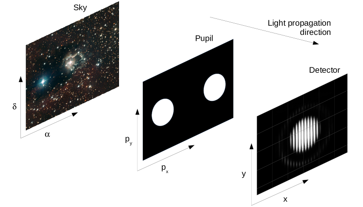
Figure 1: Notations used in this paper. The light propagates from the sky to the detector through the instrument pupil. Each plane of interest has its own coordinate system.

The light intensity at the focus of the instrument (see Fig. 1 for details) is the result of the superposition of many electromagnetic waves coming from the pupil of the instrument:

$$I(\vec{x}) = \left<\left\|\vec{E}(\vec{x},t)\right\|^{2}\right>_{t}$$ (3)

$$= \left<\left\|\sum_{i}\vec{E}(\vec{p_{i}},t-\tau_{i})\right\|^{2}\right>_{t}$$ (4)

The $i$ index represent a number of arbitrarily chosen points in the plane of interest. $\vec{x}$ is the 2D coordinate vector onto the focal plane, screen or detector. For example, $\vec{p_{i}}$ is the coordinate vector onto the pupil plane. $\tau_{i}$ represents the propagation delay between the different incoming electromagnetic waves.

When the pupil is split like in Fig. 1, it is convenient to define $\vec{B}$ the separation vector between the sub-pupils. This vector, or its length, is often called “baseline”.

If one considers a point-source light emitter (i.e. the wavefront at the entrance pupil is a plane), this expression can be integrated onto the pupil, instead of summed as in eq. 4 to see what the shape of the intensity in the image plane is.

For example, in the case of a round pupil of diameter $D$, the light intensity will follow an Airy pattern (see the demonstration in Perez [1988] page 288), which writes:

$$I(\rho) = \left(\frac{\pi D^{2}}{4}\right)^{2}\left[\frac{2J_{1}(\pi\rho D)}{\pi\rho D}\right]^{2}$$ (5)

with $\rho=\|\vec{x}\|$ and $J_{1}$ the 1^st order Bessel function. An illustration of different pupils and the associated PSF is shown in Figure 2. The consequence is that a point-source does not appear as a point source through a telescope or instrument, owing to the Rayleigh criterion (the factor 1.22 comes from the first zero of the Bessel function). An instrument is therefore limited in angular resolution by the diameter (or maximum baseline) of its aperture.

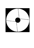
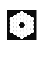
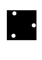
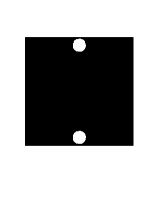
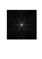
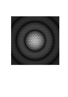
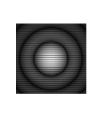
Figure 2: Top, from left to right: Simulated apertures for different instruments with similar angular resolution ; round pupil ; VLT pupil ; Keck pupil ; 3 telescopes interferometer ; 2 telescopes interferometer. Bottom, from left to right: The corresponding PSF

3.2 Diluted or masked-aperture PSF and U-V plane

An interferometer, or a pupil-masking instrument, is a set of multiple telescopes (or apertures $D$) which are combined together to form interference patterns on a given common source, represented by its sky-brightness distribution $S_{\lambda}(\alpha,\delta)$. For convenience, one will always considers that the pupils are infinitely small, and they are identified by their indices $i$ or $j$.

The interferometer is sensitive to the incoming light coherence, measured by the mutual coherence function. This function is defined as the correlation between two incident wavefronts $\vec{E}$ coming from positions $\vec{p_{i}}$ and $\vec{p_{j}}$. The two beams of light from each positions have a delay $\tau$:

$$\Gamma_{i,j}(\tau)=\left<\vec{E}(\vec{p_{i}},t-\tau)\vec{E}^{*}(\vec{p_{j}},t)\right>_{t}$$ (6)

The light intensity can then be developed as a function of $\Gamma$ from eq 3:

$$I(\vec{x})=\sum_{i}\Gamma_{i,i}(0)+\sum_{i,j}\Gamma_{i,j}(\tau_{j}-\tau_{i})+{\Gamma_{i,j}}^{*}(\tau_{j}-\tau_{i})$$ (7)

One can note here that the terms $\Gamma_{i,i}(0)$ are just the light intensity $I_{i}(\vec{x})$, as if there was only one unperturbed source of light. The delays $\tau_{i}$ are set as a function of the origin of the two wavefronts, and of the configuration of the instrument (used optics, focal length, etc.) and, in the focal plane of the instrument, both depend only on the coordinates in that plane. Let us pose $\tau_{j}-\tau_{i}=\tau$. When dealing with 2 wavefronts, just like in an interferometer, the equation 7 simplifies in:

$$I(\vec{x}) = I_{1}(\vec{x})+I_{2}(\vec{x})+\Gamma_{1,2}(\tau)+{\Gamma_{1,2}}^{*}(\tau)$$ (8)

If one normalises the term $\Gamma_{i,j}$ by the total flux, this defines the complex coherence degree $\gamma_{1,2}(\tau)$:

$$\gamma_{1,2}(\tau)=\frac{\Gamma_{1,2}(\tau)}{\Gamma_{1,1}(0)+\Gamma_{2,2}(0)}$$ (9)

When considering a 1D-interferogram with abscissa $x$ (for example when one axis is anamorphosed in order to feed it into a spectrograph), equation 8 becomes:

$$I(x) = \left[I_{1}(x)+I_{2}(x)\right]\left[1+\Re\left(\gamma_{1,2}(\tau)\right)\right]$$ (10)

$$= \left[I_{1}(x)+I_{2}(x)\right]\left[1+\mu^{\rm obj}_{1,2}\cos\left(\frac{2\pi x}{\lambda}+\phi^{\rm obj}_{1,2}\right)\right]$$ (11)

$\mu$ being the modulus of $\gamma_{1,2}(0)$ and $\phi$ its phase ($\gamma_{1,2}(0)=\mu\mathrm{e}^{\i\phi}$). The cosine modulation corresponds to the intensity fringes that an optical interferometer measures. Eq. 11 and its variants is often referred as “the interferometric equation”, and describes the intensity interference pattern (or interferogram) as seen on a screen or detector. $\mu$ and $\phi$ are often called the visibility or contrast, and phase of the interferogram, respectively. An illustration of this equation can be seen in Figure 4, left. The $x$ variable is a length corresponding to the delay difference between the two recombined beams. It can be directly projected on the detector, as is done in a multiaxial instrument, or a time-modulated variation of $x=v_{\rm mod}\times t$ can be introduced as is often done in a coaxial instrument (see e.g. Berger et al. [1999], or the paper in this book: Berger [2015] for more details).

This equation, with minor modifications (due to the flux envelope of the slits) also drives the well-known Young’s two-slit experiment.

4 Light source and light coherence

With the Young’s experiment, a simple test to do is to change the physical size of the source by e.g. putting a varying-size diaphragm in front of it. When the source’s size changes, one can observe that the fringe contrast also changes, and there are specific sizes at which the fringes completely wash out. We saw in the previous sections the intensity function of an interferometer in the case of a point source. Here I will detail a little what happens when the source is resolved by the instrument or interferometer.

This is where the Zernicke and van Cittert (ZVC) theorem comes into light, linking the value of $\gamma_{1,2}(0)=\mu^{\rm obj}_{1,2}\mathrm{e}^{\i\phi^{\rm obj}_{1,2}}$ to the object’s shape projected onto the plane of sky:

For a non-coherent and almost monochromatic extended source, the complex visibility is the normalised Fourier transform (hereafter FT) of the brightness distribution of the source.

Or written in a mathematical way:

$$\gamma_{1,2}(0) = \frac{\iint_{-\infty}^{\infty}S(\alpha,\delta)\mathrm{e}^{-2i\pi(u\alpha+v\delta)}\,d\alpha\,d\delta}{\iint_{-\infty}^{\infty}S(\alpha,\delta)\,d\alpha\,d\delta}$$ (12)

$$= \frac{FT(S)}{S^{\rm tot}}$$ (13)

with here $S(\alpha,\delta)$ is the brightness distribution of the source at angular coordinates $\alpha$ and $\delta$, $u$ and $v$ are the spatial frequencies at which the Fourier Transform is computed. The demonstration of this theorem can e.g. be found in Born & Wolf ([1999]). And here is why Fourier-transforms are so important to interferometry!

		Object
		point source	small	large
		Image
Interferometer
Full pupil

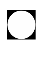
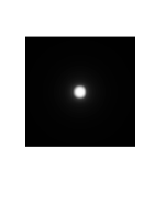
Figure 3: Top, from left to right: Simulated round objects of different diameters. Middle-left: Reproduction of the 2 telescope interferometer pupil. Middle: Fringe pattern for the different object sizes. Note the fringe contrast change. Bottom-left: Reproduction of the ideal round pupil. Bottom: corresponding image. Note the disappearance of the Airy rings when the object is resolved.

The direct consequence of this theorem is that the fringe contrast and phase are related to Fourier Transforms: the larger the object, the lower will be the contrast (for a “regular” object). An illustration of this effect is shown in Figure 3.

4.1 Coherent flux

As has been seen, the interferometer is sensitive in theory to the degree of coherence of light $\gamma_{i,j}(0)=\mu^{\rm obj}_{1,2}\times\mathrm{e}^{\i\phi^{\rm obj}_{1,2}}$, or complex visibility, which is given by the Zernicke and van Cittert theorem.

One needs to calculate the visibility values from the interferogram signal. As this signal has a cosine modulation, one way to extract its amplitude and phase is to apply a Fourier Transform and calculate the power at the modulation frequency $f_{\rm i,j}$ (See Fig. 4). The observed $\gamma_{i,j}(0)$, noted with “$\widetilde{\gamma_{i,j}(0)}$” is:

$$\widetilde{\gamma_{i,j}(0)}=\frac{N_{\rm bases}{\rm FT}_{f_{\rm i,j}}\left[I(x,\lambda)\right]}{{\rm FT}_{0}\left[I(x,\lambda)\right]}$$ (14)

with $N_{\rm bases}=\frac{N_{\rm tel}(N_{\rm tel}-1)}{2}$. This equation contains the approximation that the two fluxes $I_{1}(\vec{x})$ and $I_{2}(\vec{x})$ are equal. The case where $I_{1}(\vec{x})$ and $I_{2}(\vec{x})$ are not equal is treated later in this book (ten Brummelaar [2015]).

This method is often called the Fourier method, but note that it has nothing to do with the ZVC theorem (eq. 13), as it is just a way to actually measure the visibility.

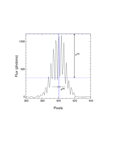
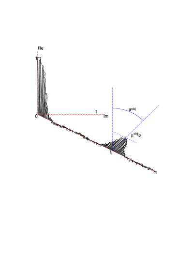
Figure 4: Left: A simulated fringe pattern for a typical multiaxial interferometer, with the representation of where the fringe contrast and phase can be measured. Right: The Fourier Transform of that fringe pattern exhibits two peaks: one at zero frequency, representing the total flux, and one at frequency $f_{i,j}$ representing the fringe contrast. Note that the white noise from the data appears as “grass” in the Fourier Transform.

Another way is to measure the amplitude of the fringes in the image space, for example, one can measure one fringe at 4 different points $A,B,C,D$ each one separated to each other in phase by $\pi/2$ (see Fig. 5). The visibility amplitude can be computed this way:

$$\widetilde{\mu}=\frac{\sqrt{(I_{A}-I_{C})^{2}+(I_{B}-I_{D})^{2}}}{2\sum_{j}I_{j}}$$ (15)

and the visibility phase:

$$\widetilde{\phi}=\arctan\left(\frac{I_{A}-I_{C}}{I_{B}-I_{D}}\right)$$ (16)

One needs to note here that the ABCD method relies on the knowledge of the shape of the fringes (a cosine function) and on the fact that the A,B,C and D samples are exactly offset by $\pi/2$. A generalisation of that method, called p2vm (Millour et al. [2004], Tatulli et al. [2007]), was proposed and implemented on the amber instrument (Petrov et al. [2007]). The basic idea is to use the a priori information of the fringes shape to adjust a model to the data in order to obtain the visibilities. The method is thoroughly described in Tatulli et al. ([2007]).

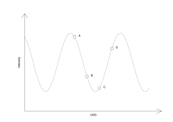
Figure 5: Principle of the ABCD method: 4 measurements are made onto one single fringe, dephased by $\pi/2$ each, owing to the fringe contrast and phase.

To get an overview and understanding of how to reduce data for a specific instrument, it is always better to read the corresponding paper. For example Mourard et al. ([2011]) for the chara/vega instrument, Petrov et al. ([2007]) for the vlti/amber instrument, ten Brummelaar ([2015]) for chara/classic, Perrin ([2003a], [2003b]) for chara/fluor and vlti/vinci, etc.

4.2 The $(u,v)$ problem

One very specific problem of optical long-baseline interferometry is called the “$(u,v)$ problem”. It is related to the sparsity of measurements the interferometers can provide. Indeed, contrary to classical imaging, a two telescopes interferometer measurement samples only one point in the frequency domain of equation 13, usually noted $(u,v)$ plane. More details are given in Millour ([2008]), therefore I will just recall the different ways to fill the $(u,v)$ plane:

Supersynthesis:

The rotation of Earth relative to the celestial sphere makes the baseline change with time. The $(u,v)$ tracks are on an arc of ellipse. The exact expression of the $(u,v)$ tracks is given in Segransan ([2007]) and recalled in Millour ([2008]).

Add more telescopes:

The number of $(u,v)$ points for one measurement is equal to the number of baselines, roughly proportionnal to the square of the number of telescopes, following the relation $N_{\rm bases}=\frac{N_{\rm tel}(N_{\rm tel}-1)}{2}$

Make use of wavelength:

The spatial frequencies are proportionnal to the wave number $\sigma=1/\lambda$ and trace radial lines in the $(u,v)$ plane.

An illustration of these is shown in Table 1 for the future matisse/vlti instrument (Lopez et al. [2006]) in the L band (3$\mu$m).

Table 1: The different ways of filling the $(u,v)$ plane, illustrated by matisse observation in the L band (3.5–4.1$\mu$m) of the star $\gamma^{2}$ Velorum (declination $-47^{o}$). “2T” means “2 Telescopes”, “4T” means “4 Telescopes” and “4T+conf” means “4 Telescopes and change of configurations”, i.e. the best situation at vlti today

	Single measurement	Wavelength coverage	Supersynthesis	Supersynthesis
				+ Wavelength coverage
2 T
4 T
4 T + conf

4.3 The phase problem

So, we have a way to measure the complex visibility. However, the actual measurement of the fringes is affected by a series of effects we detail here, and we explain a set of workarounds on how to measure the amplitude $\mu$ and phase $\phi$ of the object of interest. The effects can be classified into visibility attenuation factors $A\leq 1$ and phase factors $\phi$. The following list is ordered by decreasing magnitude on the observables:

• The atmospheric turbulence adds a phase term $\phi^{p}$ between the telescopes, sometimes called “atmospheric piston” because it comes from a change in the optical path difference $\delta(t)$ between the two telescopes. This term varies as $\phi^{p}_{\lambda}(t)=2\pi\delta(t)/\lambda$ as a first approximation (see an example phase shape in Fig. 6).

• Atmosphere also puts higher-order terms (like the tip/tilt effect) which will affect the instantaneous flux $I_{1}$ and $I_{2}$. It can also affect other terms due to the speckle pattern (Mourard et al. [1994]) but today most of the combiners use optical fibers to wash out this effect, so we will not detail it here.

• A finite exposure time can also be of trouble, as it transforms the phase term variations ${\sigma_{\phi}}^{p}$ into contrast variations $A({\sigma_{\phi}}^{p})=\mathrm{e}^{-\sigma^{2}_{\phi}}$ (Tatulli et al. [2007]).

• Chromatic longitudinal dispersion makes the optical path delay $\delta(t)$ dependent of wavelength $\delta_{\lambda}(t)$. This effect is explained in details in Tubbs et al. ([2004]) and Vannier et al. [2006].

• Polarisation effects, either in the beam feeding or inside the instrument can make the contrast time-variable and even kill it. The contrast variation due to polarisation is noted: $A(\Delta_{\pi})$. This is due to a difference of speed propagation between the two linear polarisations (birefringence effect) due to asymmetric setups or birefringent materials in the instruments (e.g. optical fibres). One can then extinct one of the polarisation to avoid this effect by using a linear polarizer, or an elegant solution is to introduce a birefringent plate with relevant properties to compensate for this effect (Lazareff et al. [2012]).

In addition to these effects, more fundamental effects like photon noise $\sigma_{\phi}$ or detector noise $\sigma_{\rm det}$, grouped in additive noises $b$, need to be taken into account. To summarize, one can include all these effects into the interferometric equation 11 and consider an arbitrary number of telescopes $Ntel$, which can be written as:

$$I = \sum_{j=1}^{\rm Ntel}I_{j}$$ (17)

$$+ \sum_{k=1}^{\rm Ntel-1}\sum_{j=k+1}^{\rm Ntel}I_{j}I_{k}A({\sigma_{\phi}}^{p})A(\Delta_{\pi})A(\delta)\mu^{\rm obj}_{j,k}\cos\left(\frac{2\pi}{\lambda}(x+\delta)+\phi^{\rm obj}_{j,k}\right)$$

$$+ b$$

where $j,k$ are telescope indices; $x$ is a space coordinate; $\lambda$ is the wavelength; $\mu^{\rm obj}_{j,k}$ and $\phi^{\rm obj}_{j,k}$ are the object’s visibility and phase; $\delta$ is the atmospheric optical path difference (OPD), varying with time (see Fig. 6). All the beam intensity terms $I_{j}$ and $I_{k}$ depend on space $x$, wavelength $\lambda$, and time $t$; $A({\sigma_{\phi}}^{p})$ is an attenuation factor coming from the finite exposure time of each frame, and depends on the atmospheric conditions, or the fringe tracker performances; $A(\delta)$ is an attenuation factor dependent of the spectral resolution of the instrument and the value of the OPD $\delta$; $A(\Delta_{j,k})$ is an attenuation factor depending on the polarization state of both contributiong beams; finally, $b$ is a zero-mean noise.

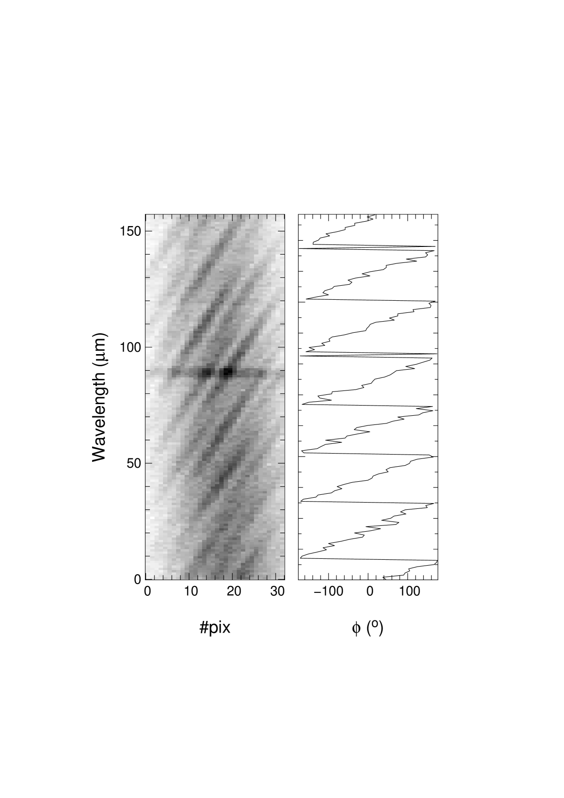
Figure 6: From left to right: example amber spectrally dispersed fringes, the corresponding phase, and a time-sequence of OPD from Tatulli et al. ([2007]). Reproduced with permission.

The consequence of the phase problem is that the object phase cannot be measured directly. The following section provides some guidelines on how to cope with this fact.

5 Observables

The goal of observables is to extract the relevant information, i.e. $\mu_{o}$ and $\phi_{o}$ from the somewhat perturbed equation 17 compared to eq. 11.

5.1 Squared visibility

One way to minimise the turbulence effect of the phase on the visibility is to take profit of the developments made for speckle interferometry in the 70’s (Labeyrie [1970]). Indeed, the modulus of the instantaneously-measured complex visibility can be computed and averaged over time, minimising the effects of phases fluctuations. To simplify the calculations, one can remove the square root of the modulus, hence calculating squared modulus. With the Fourier method, this gives:

$$\widetilde{\mu^{2}}=\left\|\frac{N_{\rm bases}{\rm FT}_{f_{\rm i,j}}\left[I(x,\lambda)\right]}{{\rm FT}_{0}\left[I(x,\lambda)\right]}\right\|^{2}$$ (18)

Here one can see that most of the phase effects wipe out from this visibility estimate, but there are a number of issues related to it:

• Additive noises can lead to biases (see how to treat them in Perrin [2003b], and also in this book: ten Brummelaar [2015]),

• The multiplicative terms $A({\sigma_{\phi}}^{p})$, $A(\delta)$, and $A(\Delta_{\pi})$ in eq. 17 do not wipe out from the estimator, making calibration a very acute issue for this type of estimator (See for example Millour et al. [2008]).

In terms of error estimate, the squared visibility method has a well-documented bibliography and I would suggest reading one of these papers: Tatulli et al. ([2007]), Petrov et al. ([2007]), or ten Brummelaar [2015]).

5.2 Differential visibility, coherent visibility

Another way to minimize turbulence on the visibility measurement (the terms $\frac{2\pi}{\lambda}\delta$ and $A({\sigma_{\phi}}^{p})$) is to wipe it out explicitely.

In other words, as shown in Fig. 6, the phase as a function of $\lambda$ exhibits a “slope”, directly related to OPD. This provides us a way to measure $\widetilde{\delta}$. The coherent flux $\widetilde{\gamma_{i,j}(0)}$ of eq. 14 can be corrected from the associated phase term, and its real part averaged.

$$\widetilde{\mu}=\Re\left[\widetilde{\gamma_{i,j}(0)}\times\exp^{-\frac{2\i\pi}{\lambda}\widetilde{\delta}}\right]$$ (19)

This estimator of visibility is calculated by the midi pipeline (Koehler et al. [2008]) and is planned to be implemented in the matisse instrument too. It is often called “coherent visibility” or “linear visibility”. Many aspects are not treated here (like e.g. time-averaging) as these are pure signal processing aspects (you can refer to Papoulis [2002] to see how time-averaging of the quotient of two random variables can be done) and they would be too long to describe here.

To overcome the $A({\sigma_{\phi}}^{p})$ term, supposedly wavelength-invariant, it may be convenient to divide the above estimate of visibility by its wavelength-average. This provides a visibility measurement whose average value is 1 and whose variations with respect to wavelengths are kept. It is then called “differential visibility” as its variations are only relevant relative to a virtual reference wavelength (also called “reference channel”).

$$\widetilde{\mu}^{\rm diff}=\frac{\widetilde{\mu}}{<\widetilde{\mu}>_{\lambda}}$$ (20)

Two flavors of differential visibility may be computed:

• normalizing the squared visibility of eq. 18 by its wavelength-average.

• normalizing the linear visibility of eq. 19 along $\lambda$.

The first method was used in the early times of amber. The second method is the one proposed today in the amber data reduction software, and also on vega. It will be proposed also for matisse. I would suggest reading the papers Millour ([2006]) and Mourard et al. ([2009]) for more information.

5.3 Closure phase

The phase $\phi^{\rm obj}_{j,k}$ of the object is usually considered as lost when going through the atmosphere. However, a phase measurement out of 3 telescopes was invented for radio-astronomy (Jennison [1958]), called “closure phase”. This closure phase has extremely interesting properties in that it washes out the atmospheric disturbances from the phases.

Let us call $1,2,3$ the three telescopes of interest. The object’s phases are, according to the ZVC theorem, linked with each baselines $\phi_{1,2}^{\rm obj}$, $\phi_{2,3}^{\rm obj}$, and $\phi_{3,1}^{\rm obj}$. On the other hand, the atmospheric disturbances affect the phase of the wavefront prior each telescope, hence the atmospheric phases can write $\phi^{\rm atm}_{1}$ $\phi^{\rm atm}_{2}$ $\phi^{\rm atm}_{3}$. Baseline-wise, the phases can be expressed then:

$$\Phi_{1,2} = \phi_{1,2}^{\rm obj}+\phi^{\rm atm}_{2}-\phi^{\rm atm}_{1}$$ (21)

$$\Phi_{2,3} = \phi_{2,3}^{\rm obj}+\phi^{\rm atm}_{3}-\phi^{\rm atm}_{2}$$ (22)

$$\Phi_{3,1} = \phi_{3,1}^{\rm obj}+\phi^{\rm atm}_{3}-\phi^{\rm atm}_{1}$$ (23)

When summing the phases from the three baselines, the atmospheric disturbances disappear and the summed phase becomes:

$$\Psi_{1,2,3}=\phi_{1,2}^{\rm obj}+\phi_{2,3}^{\rm obj}+\phi_{3,1}^{\rm obj}$$ (25)

This is called the closure phase. However, one cannot simply sum the phases, as the phase noise is usually very large compared to $60^{o}$ (or 1 rad). The phases histogram can therefore be very far from a pristine Gaussian distribution, often close to an uniform distribution. The corresponding phase-wrapping effect is illustrated in Fig. 7.

Figure 7: Illustration of the phase wrapping effect, showing the transition of phases histograms from almost Gaussian to a nearly uniform distribution. The top part shows the real and imaginary parts of the complex values, while the lower part shows the corresponding phase histograms. The three first panels are synthetic data, while the last one is actual very high signal-to-noise ratio amber data.

The way to compute it as an observable is to compute the bispectrum directly in the complex plane, average it and then take the phase:

$$\widetilde{\Psi_{1,2,3}}=\arg{\left<{\rm FT}_{f_{\rm 1,2}}\left[I(x,\lambda)\right]\times{\rm FT}_{f_{\rm 2,3}}\left[I(x,\lambda)\right]\times{\rm FT}_{f_{\rm 3,1}}\left[I(x,\lambda)\right]\right>_{t}}$$ (26)

When the three visibilities on the three baselines have similar values, the closure phase noise is just $\sqrt{3}$ higher than the true phase noise. However, this is not true at all when the three baselines have very different visibility amplitudes (for example when one baseline is exactly in a zero of visibility). In such a case, the closure phase noise is approximately equal to the highest phase noise from the three baselines. One can refer to Chelli et al. ([2009]) for more information.

For details on what means the closure phase, and how to interpret it, please read section 6.

5.4 Differential phase

5.4.1 How to get it

“Differential phase” can mean many things: the phase difference between the two telescopes (what has been called “phase” in this paper), the phase difference between two offset positions (also referred as “phase referencing”), the phase difference between two separated beams (Aime et al. [1986]), or the phase difference between two adjacent wavelengths, introduced by Beckers ([1982]). We will not talk about the three first phases, but explain here the last one which had quite some applications in the last decade for optical interferometry.

If we take a look to the phase term in eq.17, we note it is made primarily of two components:

$$\phi_{i,j}(\lambda)=\phi^{\rm obj}_{i,j}(\lambda)+\frac{2\pi\delta(t)}{\lambda}+o\left(\frac{1}{\lambda}\right)$$ (27)

These two components are the object’s phase $\phi^{\rm obj}_{i,j}(\lambda)$, basically fixed as a function of time (if there is no baseline smearing) but possibly varying as a function of wavelength (for example inside an emission line, or as a function of spatial frequency), and the OPD term $\frac{2\pi\delta(t)}{\lambda}$ strongly varying as a function of time. All higher-order terms (like the water vapor term) are contained within the term $o(\frac{1}{\lambda})$.

If one is able to estimate properly the OPD term, it can be subtracted from the individual phase measurements, and the remaining phase variations as a function of wavelength can be averaged. To avoid wrapping effects in presence of noise, this procedure must be done in the complex plane, by computing a cross-spectrum:

$$W^{\rm noP}=\widetilde{\gamma_{i,j}(0)}\times\mathrm{e}^{-2\i\pi\frac{\delta(t)}{\lambda}}$$ (28)

We note here that we remove only the achromatic OPD effect, but as mentionned in page • ‣ 4.3, other effects can also affect the phase. They are present essentially as a phase offset plus higher order terms. The phase offset can be removed by computing phase differences between the current wavelength (called “work channel”) and another wavelength (called “reference channel”, bearing many similarities to the one used for differential visibility), i.e.:

$$\widetilde{\phi^{\rm diff}}=\arg\left<W^{\rm noP}(\lambda_{\rm work})W^{\rm noP}(\lambda_{\rm ref})\right>_{t}$$ (29)

One can note here that equations 28 and 29 can be swapped in the process without any issue.

The reference channel can be computed by taking one wavelength, or by averaging several wavelengths. The most used method is to compute the reference channel with all but one of the wavelengths (to avoid introducing a quadratic bias). The differential phase can be related to the object phase according to the following equation:

$$\widetilde{\phi^{\rm obj}_{i,j}}=\frac{N_{\lambda}-1}{N_{\lambda}}\phi^{\rm diff}_{i,j}+\frac{\alpha}{\lambda}+\beta$$ (30)

where $N_{\lambda}$ is the number of wavelengths in the reference channel, and “1” is the one wavelength in the work channel. The small multiplicative factor $\frac{N_{\lambda}-1}{N_{\lambda}}$ has to be taken into account due to the definition of the reference channel, as detailed in Millour ([2006]) page 91. Usually, this factor is negligible, as most today spectro-interferometric instruments have 100’s of channels, but it may be large-enough for wideband instruments to be considered. The two terms $\alpha$ and $\beta$ are lost in the process, but may be recovered by using the self-calibration method (see Sect. 6.4.2).

6 Interpreting interferometric data

What has been described in the previous sections is how to obtain interferometric data, but no word has been written about how to interpret these data. The goal of this section is to see how to compare interferometric measurements with a model, the image reconstruction part being treated in a separated article (Young & Thiébaut [2015], this book). We divide this section in two sub-sections: qualitative interpretation of data (“first sight” interpretation) and quantitative interpretation, with a few examples of implementations.

6.1 First-sight interpretation

6.1.1 Description of observables

Interferometer data usually come as Optical Interferometry Flexible Image Transport System (OIFITS) data files, which are based on the FITS format. For more information on the OIFITS specifications, see Pauls et al. ([2004, 2005]). Most of the time, an OIFITS file contains squared visibilities, plus optionally closure phases and/or differential visibilities and differential phases, depending on the instrument used.

These different observables provide already some information on the object. Table 2 presents some simple examples of the considerations you can make at “first sight”. For example, a visibility close to 1 is measured with a 130 m baseline in the near-infrared for an object much smaller than 2 mas, i.e. smaller than the angular resolution $\theta_{\mathrm{res}}\simeq\lambda/B$.

More generally,

The visibility

value indicates whether the object is resolved (low visibility) or not (visibility close to 1).

The differential visibility

is a relative measurement of the object size along wavelengths. A lower differential visibility in an emission line indicates an emitting region larger than in the continuum.

The phase

is sensitive to astrometric position of a given source. As such, it provides both information on the asymmetry (skewness of the intensity distribution) of the object and its photocenter (astrometry).

The closure phase

gives the information whether the object is asymmetric (skewness): a zero or $\pi$ closure phase may correspond to a symmetric object (but not in 100% of the cases), whereas a non-zero closure phase (modulo $\pi$) indicates for sure an asymmetric object. The astrometric position is lost in the closure phase signal.

The differential phase

is sensitive to the astrometric position at one wavelength relative to another wavelength. Therefore, astrometric shifts in emission lines can be measured with it, or, if a large chunk of wavelength is available, it allows one to scan phase across spatial frequencies for an achromatic object (like a binary star for example). It contains also the information of the closure phase wavelength-variations, the only relevant information coming from closure phase being then its wavelength-average value.

A few example of qualitative features seen on the above observables and their signification are provided in Table 2.

Table 2: Qualitative information which can be retrieved from interferometric observables.

Observable	Value or features	Qualitative information	Model-fitting guidelines	Illustration
				Table 3
Visibility	Close to 0	Object $\diameter\gg 1.22\lambda/B$ rad	Add a resolved component	(a)
	Close to 1	Object $\diameter\ll\lambda/B$ rad	Uniform disk size	(e)
	Cosine shape	Binary star!	Use a binary model	(i)
Diff. vis.	$\searrow$ in an emission line	Bigger emission	Add an emitting envelope	(c)
	$\nearrow$ in an emission line	Smaller emission	Add an inner region/disk	(g)
	$\searrow$ in an absorption line	Central object in absorption	Absorbing central object
	$\nearrow$ in an absorption line	Shell in absorption	Absorbing shell
Clos. phase	$\neq 0^{\circ}$ and $180^{\circ}$	Asymmetric object	Add a point source	(f)
	$=0^{\circ}$ or $180^{\circ}$	Object possibly symmetric	-	(b)
Diff. phase	Sine shape	Binary star!	Use a binary model	(k)
	“S” shape in a line	Object is rotating!	Use a kinematic model	(h)
	“V” shape in a line	Asymmetric object in line	See Weigelt et al. ([2007])	(d)
	“W” shape in a line	A bipolar outflow?	See Chesneau et al. ([2011])	(j)

Table 3: The optical long-baseline interferometric “observables zoo”, showing all the different cases one can face with current spectro-interferometric instruments, illustrated with actual published interferometric data. The letters link to the Table 2. Reproduced with permission.

Visibility	Closure phase	Diff. Vis.	Diff. Phase
(a) Resolved source	(b) Zero	(c) $\searrow$ in emission line	(d) “V” shape
Benisty et al. ([2010])	Monnier et al. ([2006])	Stee et al. ([2012])	Weigelt et al. ([2007])
(e) Unresolved source	(f) Non-zero	(g) $\nearrow$ in emission line	(h) “S” shape
Demory et al. ([2009])	Monnier et al. ([2006])	Kraus et al. ([2008])	Meilland et al. ([2012])
(i) Cosine shape		(j) “W” shape	(k) Sine shape
Meilland et al. ([2011])		Chesneau et al. ([2011])	Meilland et al. ([2011])

6.1.2 What can I do without a model?

Already a significant amount of things! The visibility, closure phase and differential phase provide already a large number of information about the geometry of an object.

In practice, two quantitative information can be extracted from the visibilities and differential phases without a model:

• Size estimate with the visibilities (if the visibility is larger than 20%), using simple ad-hoc models (like uniform disks: Demory et al. [2009]), Gaussian disks: Tristram et al. [2007], or even rings: Kishimoto et al. [2011],

• Photocentre $p$ variations with the differential phase, or spectro-astrometry, using the simple relation $\phi=2\pi pB/\lambda$ when an object is unresolved.

However, one needs to bear in mind that these quantitative estimates are valid only when the object is barely resolved. For more details, please read Lachaume ([2003]). In all other cases, on needs to use a model-fitting tool like LITpro (Tallon-Bosc et al. [2008]), fitOmatic (Millour et al. [2009]), or SIMTOI (Kloppenborg et al. [2012])

6.2 Quantitative Interpretation: model-fitting

When one has a model $m_{i}$ of an object, with parameters $p$, and wishes to compare it with the data acquired, one needs to quantify how the model matches the data. This match is perfect when the synthetic observables computed from the model $m_{i}(p)$ are equal to the observations, described by the measurements $x_{i}$:

$$\forall i,x_{i}=m_{i}(p)$$ (31)

However, this never happens due to the presence of noise. One way to best match the model to the data is to compute squared differences between $m_{i}(p)$ and $x_{i}$, taking into account the noise $\sigma_{i}$:

$$\chi^{2}=\sum_{i}\frac{(x_{i}-m_{i}(p))^{2}}{\sigma_{i}^{2}}$$ (32)

Minimizing this quantity by changing the parameters values $p$ provide a plausible solution to the eq. 31. This minimization is made by an optimization algorithm, and the whole process is called “model-fitting”.

Specific aspects of long-baseline interferometry, like the use of wrapped phases (see Fig. 7), heterogeneous data noise models (Schutz et al. [2014]), or highly non-convex $\chi^{2}$, need to be taken into account. This is why specific software have been developed to cope with it. They are basically made of an OIFITS reader combined with a simplified instrument model, and they make use of different optimizers going from simple descent algorithms up to simulated annealing, or MCMC methods.

The whole process is described for the specific case of LITpro in Tallon-Bosc et al. ([2008]). You can also have a look to the practice sessions in this book using LITpro (Domiciano [2015]).

The model itself $m_{i}(p)$ may be a simple analytic model (“toy” model, described in sect. 6.2.1), very fast to compute, or an image coming from a more advanced model (described in Sect. 6.2.2).

6.2.1 Analytic models

The space distribution of light may be described by simple analytical functions, as is the associated visibility. Due to the Zernicke & van-Cittert theorem, these visibility functions are the Fourier transforms of the image functions. The most common analytical functions are given in table 4 and provide already a quite complete overview of what is used nowadays to interpret interferometric data.

Table 4: Analytical models of different shapes and their associated visibility function. The following parameters are used: $\diameter$ represents either the diameter for a ring or uniform disk, or FWHM. $r$ or $\vec{x}$ represent the angles in the image plane. $\rho=\frac{B}{\lambda}$ or $\vec{\rho}$ are the spatial frequencies.

Shape	Brightness distribution	Visibility
Point source	$\delta(\vec{x})$	$1$
Background	$I_{0}$	$\left\{\begin{array}[]{ll}1&\mbox{if }\rho=0\\ 0&\mbox{otherwise}\\ \end{array}\right.$
Binary star	$I_{0}\left[\delta(\vec{x})+R\delta(\vec{x}-\vec{x_{0}})\right]$	$\sqrt{\frac{1+R^{2}+2R\cos\left(\frac{\vec{\rho}\cdot\vec{x_{0}}}{\lambda}\right)}{1+R^{2}}}$
Gaussian	$I_{0}\sqrt{\frac{4\ln\left(2\diameter\right)}{\pi}}\times\mathrm{e}^{-4\ln 2\frac{r^{2}}{\diameter^{2}}}$	$\mathrm{e}^{-\frac{\left(\pi\diameter\rho\right)^{2}}{4\ln 2}}$
Uniform disk	$\left\{\begin{array}[]{ll}\frac{4}{\pi\diameter^{2}}&\mbox{if }r<\frac{\diameter}{2}\\ 0&\mbox{otherwise}\\ \end{array}\right.$	$\frac{2\mbox{J}_{1}\left(\pi\diameter\rho\right)}{\pi\diameter\rho}$
Ring	$\frac{1}{\pi\diameter}\delta\left(r-\frac{\diameter}{2}\right)$	$\mbox{J}_{0}(\pi\diameter\rho)$
Exponential	$\mathrm{e}^{-k_{0}r}$, $k_{0}\geq 0$	$\frac{k_{0}^{2}}{1+k_{0}^{2}\rho^{2}}$
Any circular object	$I(r)$	$2\pi\int_{0}^{\infty}I(r)\mbox{J}_{0}(2\pi r\rho)rdr$
Pixel (image brick)	$\left\{\begin{array}[]{ll}\frac{1}{lL}&\mbox{if }x<l\mbox{ and }y<L\\ 0&\mbox{otherwise}\\ \end{array}\right.$	$\frac{\sin(\pi xl)\sin(\pi yL)}{\pi^{2}xylL}$
Limb-darkened disk	$\left\{\begin{array}[]{ll}I_{0}[1-u_{\lambda}(1-\mu)]&\mbox{if }r<\frac{\diameter}{2}\\ \mu=cos(2r/\diameter)&\\ \end{array}\right.$	$\left\{\begin{array}[]{ll}\frac{\left[\alpha\frac{\mbox{J}_{1}(x)}{x}+\beta\sqrt{\pi/2}\frac{\mbox{J}_{3/2}(x)}{x^{3/2}}\right]^{2}}{\left(\frac{\alpha}{2}+\frac{\beta}{3}\right)^{2}}\\ \alpha=1-u_{\lambda}\\ \beta=u_{l}\lambda\\ x=\pi\theta_{\rm LD}\frac{B}{\lambda}\\ \end{array}\right.$

with $f$, $g$ analytical functions like the ones described in table 4, $x$, $y$ are coordinates in the image plane, $u$ and $v$ are spatial frequencies, and $\alpha$ and $\beta$ are zoom & shrink factors.

All these analytical models can be added together to produce combined models. This is feasible thanks to the linearity of the Fourier Transform, and other properties described below:

6.2.2 Generic properties of Fourier Transform

Here I describe the generic properties of the Fourier transform, which can be found in any book treating FT. These properties are widely used to combine or to modify, stretch, distort, the simple analytical models provided above:

•  linearity (addition):

$FT[f+g]=FT[f]+FT[g]$,

• translation (shift):

$FT[f(x-x_{0},y-y_{0})]=FT[f](u,v)\times\mathrm{e}^{2i\pi,(ux_{0}+vy_{0})}$,

• similarity (zoom and shrink):

$FT[f(\alpha x,\beta y)]=\frac{1}{\alpha\beta}FT[f](\frac{u}{\alpha},\frac{v}{\beta})$,

• convolution (‘‘blurring’’):

$FT[f\otimes g]=FT[f]\times FT[g]$,

• $\infty$ limit (‘‘small’’ details):

$FT[f]\stackrel{{\scriptstyle\infty}}{{\longmapsto}}0$,

• $0$ limit (‘‘large’’ details):

$FT[f]\stackrel{{\scriptstyle 0}}{{\longmapsto}}1$.

These Fourier transform properties can also be used to combine more advanced models. This was for example the case of Millour et al. ([2009]), where the authors combined a series of ring models to build the pseudo-3D toy-model of a spiral nebula.

6.2.3 Advanced models

For more advanced models, which do not have a simple analytical expression, one can produce a pixellized map of the model and Fourier-transform it. Most model-fitting software allow, or are planned to allow to Fourier-transform maps of otherwise computed models. This is for example the case of ASPRO, fitOmatic, and will be in a near-future in the distributed version of LITpro.

6.3 Image reconstruction

Image reconstruction is treated in details in Young & Thiebaut ([2015]) later in this book. I invite the reader to take a look to that article.

6.4 The advent of differential phase

Differential phase has changed the panorama of possibles in long-baseline interferometry. Millour ([2006]) presented a theoretical approach to explain the potential of differential phase to bring new information, independent of a model, to model-fitting and image reconstruction. As this work in in French, I translate most of the related content here to the English reader:

6.4.1 potential in model-fitting

I was interested here to quantify the information brought by differential phases in addition to the one brought by closure phases. I took inspiration from the demonstration of Lachaume ([2003]) and considered first a N-point-sources model, but resolved by the interferometer. These sources are described by $2N_{\rm s}-2$ parameters for position (global centroid is unknown and all sources coordinates are described relative to the first one), and $N_{\lambda}N_{\rm s}$ fluxes, i.e.

$$N_{\rm param}=2N_{\rm s}-2+N_{\lambda}N_{\rm s}$$ (33)

No other hypothesis is done otherwise than observing several sources at many wavelengths simultaneously. Great.

Accounting for the number of observables will help us quantify the maximum number of sources that can be modeled $N_{\rm s\,max}$. This maximum is given by zeroing the degrees of freedom of the model-fitting problem (i.e. modelling $N_{\rm s}$ chromatic point-sources and comparing them to the interferometer data). These degrees of freedom $\mathds{D}$ are simply the difference between the number of independent observations $N_{\rm obs}$ and the number of parameters of the model $N_{\rm param}$, i.e. $\mathds{D}=N_{\rm obs}-N_{\rm param}$. Zeroing it is simply writing the equation:

$$N_{\rm obs}=N_{\rm param}$$ (34)

The users of interferometers can face four specific cases:

Full access to the complex visibility:

This is for example the case in radio-astronomy, or the dream of every single optical interferometrist. In this case, one has access to $\frac{N_{\rm tel}(N_{\rm tel}-1)}{2}N_{\lambda}$ visibilities, the same number of phases, and $N_{\lambda}$ measured fluxes (the spectrum). We therefore have:

$$N_{\rm obs}=N_{\rm tel}(N_{\rm tel}-1)N_{\lambda}+N_{\lambda}$$ (35)

Putting equations 33 and 35 into equation 34, we get:

$$N_{\rm s\,max}=N_{\rm tel}(N_{\rm tel}-1)\frac{N_{\lambda}}{(N_{\lambda}+2)}+1$$ (36)

We see here that the maximum number of sources is roughly proportional to the number of baselines (i.e. square the number of telescopes), but not to the number of wavelengths. On the wavelength side, the increase of the number of sources has an asymptotic behavior.

Visibility only:

This is the case with 2-telescopes instruments like vinci, classic, fluor or midi. In this case, one has access to $\frac{N_{\rm tel}(N_{\rm tel}-1)}{2}N_{\lambda}$ visibilities and $N_{\lambda}$ measured fluxes (the spectrum). We therefore have

$$N_{\rm obs}=\frac{N_{\rm tel}(N_{\rm tel}-1)}{2}N_{\lambda}+N_{\lambda}$$ (37)

That number is roughly half the number of eq. 35. This is expected as we measure only half the information on the object (no phases). Putting equations 33 and 37 into equation 34, we get:

$$N_{\rm s\,max}=\frac{N_{\rm tel}(N_{\rm tel}-1)}{2}\frac{N_{\lambda}}{(N_{\lambda}+2)}+1$$ (38)

Visibility and closure phase:

This is still today the most common case. In such a case, one has access to $\frac{N_{\rm tel}(N_{\rm tel}-1)}{2}N_{\lambda}$ visibilities, $\frac{(N_{\rm tel}-1)(N_{\rm tel}-2)}{2}N_{\lambda}$ closure phases and still $N_{\lambda}$ measured fluxes. Therefore,

$$N_{\rm obs}=\frac{N_{\rm tel}(N_{\rm tel}-1)}{2}N_{\lambda}+\frac{(N_{\rm tel}-1)(N_{\rm tel}-2)}{2}N_{\lambda}+N_{\lambda}$$ (39)

We therefore have the following:

$$N_{\rm s\,max}=\frac{(N_{\rm tel}-1)^{2}}{2}\frac{N_{\lambda}}{(N_{\lambda}+2)}+1$$ (40)

The same comments as before applies here, except that the term $(N_{\rm tel}-1)^{2}$ grows faster than the term $N_{\rm tel}(N_{\rm tel}-1)$ of the previous paragraph.

Visibility, closure phase and differential phase:

This is the case of amber, matisse and gravity. The observables are now $\frac{N_{\rm tel}(N_{\rm tel}-1)}{2}N_{\lambda}$ visibilities, $\frac{N_{\rm tel}(N_{\rm tel}-1)}{2}N_{\lambda}$ differential phases, $\frac{(N_{\rm tel}-1)(N_{\rm tel}-2)}{2}N_{\lambda}$ closure phases and still $N_{\lambda}$ measured fluxes. However, one has to note that closure phase and differential phase are not independent measurements. Indeed, they are both related to the object phase (see eq. 30 and eq. 25). Therefore, one can write the relation between the differential phase and the closure phase using both equations:

$$\Psi_{i,j,k}=\phi^{\rm diff}_{i,j}+\phi^{\rm diff}_{j,k}+\phi^{\rm diff}_{k,i}+\beta_{i,j}+\beta_{j,k}+\beta_{k,i}+\frac{\alpha_{i,j}}{\lambda}+\frac{\alpha_{j,k}}{\lambda}+\frac{\alpha_{k,i}}{\lambda}$$ (41)

The careful reader should have seen here that I discarded the small term $\frac{N_{\lambda}-1}{N_{\lambda}}$, which can be neglected for a large number of spectral channels. One can also note that one of the terms $\beta_{i,j}+\frac{\alpha_{i,j}}{\lambda}$ can be fixed to zero in order to set the two other offsets, and therefore fix the global photocenter of the object (which remains unconstrained by closure phases and differential phases).

This equation and the above additional constrain provide us with the relevant information: the closure phase bring only additional data on two offsets $\beta_{i,j}$ and wavelength-slopes $\frac{\alpha_{i,j}}{\lambda}$ that are missed by differential phases. All other information (wavelength variations) are contained both in closure phase and differential phases. Therefore, the closure phase provides $(N_{\rm tel}-1)(N_{\rm tel}-2)$ independent observables instead of the $\frac{(N_{\rm tel}-1)(N_{\rm tel}-2)}{2}N_{\lambda}$ accounted just before. Therefore, we get:

$$N_{\rm obs}=\frac{N_{\rm tel}(N_{\rm tel}-1)}{2}N_{\lambda}+(N_{\rm tel}-1)(N_{\rm tel}-2)+\frac{N_{\rm tel}(N_{\rm tel}-1)}{2}N_{\lambda}+N_{\lambda}$$ (42)

and the maximum number of sources that can be modeled is:

$$N_{\rm s\,max}=\frac{(N_{\rm tel}-1)(N_{\rm tel}N_{\lambda}-2)}{(N_{\lambda}+2)}+1$$ (43)

These different cases are illustrated in Fig. 8. We see that, typically above 20 spectral channels, the use of differential phases put us in a case almost similar as if there was a true phase measurement for model-fitting. This was the main motivation to develop the model-fitting tool fitOmatic, which can make use of chromatic parameters.

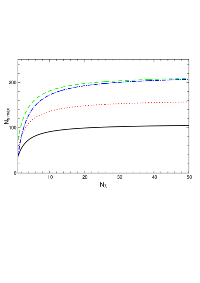
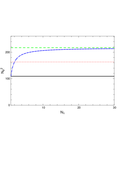
Figure 8: Illustration of the potential of using the differential phase in model-fitting or image reconstruction for 3 nights of 4 telescopes observations (like in the case of matisse) compared to other cases. Left: modelling $N_{\rm s\,max}$ point-sources, the green dashed line using visibilities and phases, the black solid line is using visibilities alone, the red dotted line using visibilities and closure phases, and finally the blue dash-dotted line using visibilities, closure phases and differential phases. Right: reconstructing a $N_{\rm p}\times N_{\rm p}$ pixels chromatic image. The colours are the same.

6.4.2 in image reconstruction

The wavelength-differential phase was not considered in imaging until Millour ([2006]), Schmitt et al. ([2009]) and Millour et al. ([2011]). Indeed, differential phase provide a corrugated phase measurement (as described in eq. 30), which, in theory, can be incorporated into a self-calibration algorithm, in a very similar way as what is done in radio-interferometry (Pearson & Readhead [1984]).

As early as [2003], J. Monnier anticipated “revived activity [on self-calibration] as more interferometers with ‘imaging’ capability begin to produce data.” And indeed, the conceptual bases for using differential phases in image reconstruction were laid in Millour ([2006]): the same reasoning as in the previous section can be applied, except that an image is made of pixels whose positions are pre-defined. The only unknown information is therefore the spectrum of each pixel. If $N_{\rm p}$ is the image size ($N_{\rm p}=128$ for a 128 x 128 image), the number of unknown $N_{\rm param}$ is equal to:

$$N_{\rm param}=N_{\rm p}^{2}N_{\lambda}$$ (44)

and the maximum number of pixels that can be reconstructed is:

Full access to the complex visibility:

$$N_{\rm p}=\sqrt{N_{\rm tel}(N_{\rm tel}-1)+1}$$ (45)

Visibility only:

$$N_{\rm p}=\sqrt{\frac{N_{\rm tel}(N_{\rm tel}-1)}{2}+1}$$ (46)

Visibility and closure phase:

$$N_{\rm p}=\sqrt{(N_{\rm tel}-1)^{2}+1}$$ (47)

Visibility, closure phase and differential phase:

$$N_{\rm p}=\sqrt{\frac{(N_{\rm tel}-1)(N_{\rm tel}N_{\lambda}-2)}{N_{\lambda}}+1}$$ (48)

Fig. 8 shows the same behavior as for model-fitting: typically above 20 spectral channels, the use of differential phases put us in a case almost similar as if there was a true phase measurement, i.e. as if there was no atmosphere in front of the interferometer, given that one is able to take profit of the information contained in the differential phase.

The Schmitt et al. ([2009]) paper was a first attempt to use differential phases in image reconstruction. They considered that the phase in the continuum was equal to zero, making it possible to use the differential phase (then equal to the phase) in the H$\alpha$ emission line of the $\beta$ Lyr system. They were able this way to image the shock region between the two stars at different orbital phases.

The paper Millour et al. [2011] went one step further, by using an iterative process similar to radio-interferometry self-calibration (Pearson & Readhead [1984]) in order to reconstruct the phase of the object from the closure phases and differential phases. This way, they could reconstruct the image of a rotating gas+dust disk around a supergiant star, whose image is asymmetric even in the continuum (non-zero phase). This method was subsequently used in a few papers to reconstruct images of supergiant stars (Ohnaka et al. [2011, 2013]). A more recent work (Mourard et al. [2014]) extended the method to the visibilities, in order to tackle the image reconstruction challenges posed by visible interferometry, lacking the closure phases and a proper calibration of spectrally-dispersed visibilities. The image-cube reconstructed with this technique in Mourard et al. ([2014]) is shown in Fig. 9.

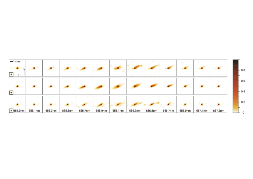
Figure 9: Image from Mourard et al. ([2014]), showing the kinematics of the $\phi$ Per Be star disk through the H$\alpha$ emission line. The top row shows the reconstructed images, the middle row a best-fit kinematics model and the lower row a reconstruction based on the model, for comparison. Reproduced with permission.

Of interest are also new developments made on the core image reconstruction algorithms to include the differential phases into the process (Schutz et al. [2014], or Soulez et al. [2014]). These new algorithms are very promising and they must be confronted sooner or later to real datasets.

7 Interferometry hardware

Combining telescopes which are hundreds of meters apart is a difficult matter, which needs a set of functions described below and shown in Fig. 11:

1. Telescopes, to collect the light, mostly defined by their diameter $D$,

2. Set of periscopes (sometimes grouped in “switchyards”) to shape, collimate, and feed the beam through light tunnels, defined by a fixed length $\Delta_{\rm fixed}$,

3. Delay lines to compensate for the variable delay due to pointing the telescope and the atmosphere’s effects, defined by a time-variable optical path length $\Delta_{i}(t)$,

4. Combiner instrument to effectively produce the interference pattern.

We will try not to repeat the numerous descriptions of how to build an interferometer. We just describe here what makes an interferometer working:

7.1 Telescopes

Interferometry telescopes are, in principle, no different from “regular” astronomical telescopes. However they differ on three aspects we will detail in the following subsections: they must be smart, tough and large.

7.1.1 “smart”

A “smart” telescope is a reliable one. Indeed, a single telescope needs to be operational (i.e. not undergoing technical failures or maintenance) most of its time.

For example, if we take the ESO telescope schedule for the Unit Telescopes on the vlti, the Observatory confidence in their telescopes is given by the ratio of observing nights scheduled by the available clear skies observing nights (Lombardi et al. [2009]: 310 nights/years at Paranal). This is illustrated by Figure 10 where we provide the number of scheduled nights (visitor or service mode) versus the average number of clear nights at Paranal. ESO usually accounts for reliable telescopes 89% of the clear sky time.

On the other hand, the vlti scheduling, illustrated in Figure 10 tells us that the ESO observatory uses 50% of the available clear sky nights, after a learning curve on the interferometer between 2003 and 2006. This is well explained if we consider all 4 telescopes are used for interferometry. The probability of having all 4 telescopes online in a given night is just $0.89^{4}\equiv 63\%$ of the available time. The difference between the two numbers (50% and 63%) comes from the numerous additional sub-systems needed by the vlti to operate (delay lines, fringe tracker, instrument, etc.).

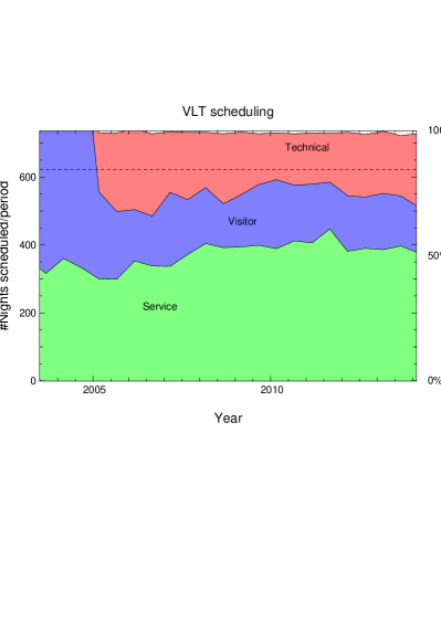
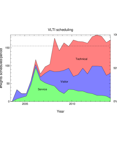
Figure 10: Left: VLT scheduling taken from the ESO telescope schedule¹, including all 4 Unit Telescopes (hence # of nights multiplied by 4). Different colours represent different times on the telescopes. The dashed line represent the clear skies night, while the dotted line represent the total number of nights over one observing period (6 months). Right: The same plot for the vlti.

A word on the “technical” time plotted here: the cumulative time, including technical one, exceeds the number of clear sky nights, since some technical activities do not need the telescope open. We also note here that the vlti technical time was not fully taken into account in the scheduling until 2008, leaving the impression that the vlti was “idle” most of the time.

7.1.2 “tough”

A “tough” telescope is a stable one. “stable” means the telescope do not transmit vibrations to the instrument. Usual instruments at the focus of telescopes are sensitive (at first order…) to transverse vibrations (i.e. “tip/tilt” vibrations). This puts some requirements on the tip/tilt pointing and stability accuracy (See for example a study in Altarac et al. [2001]).

Unfortunately, an interferometer is sensitive both to transverse and longitudinal vibrations (a.k.a. “OPD” or “piston” vibrations). Both of the large telescopes interferometers are subject to such vibrations as they were not designed in the first time to be used in an interferometer (Hess et al. [2003], Millour et al. [2008]). To overcome these effects, an active dampening system had to be integrated into both facilities (Hess et al.  [2003], Lizon et al. [2010], Poupar et al. [2010], Spaleniak et al. [2010]).

On smaller telescopes facilities, vibrations have also been investigated but this effect has a much smaller amplitude (Merand et al. [2001]).

It is worth to note that the VLT instruments are themselves affected by vibrations (Sauvage, private communication), and vibrations assessment are a part of the ELTs design.

7.1.3 “large”

“Large” telescopes means large collecting area, means more sensitive interferometer. However, one needs to bear in mind that the gain in sensitivity is true only for a constant strehl ratio of the telescope PSF, simply because the overall effective transmission of the system, when using optical fibres, is multiplied by the strehl ratio. This is why very large telescopes interferometers (vlti & Keck) have been equipped with adaptive optics (Arsenault et al. [2003]).

7.2 Feed through

The light is fed by a series of mirrors from the telescope to the delay lines building. This is where a large part of the light propagation occurs in the interferometer and where potentially several issues can happen to the beam. Three possibilities exist today to transport the beam:

• through air (e.g. in vlti and Keck-I),

• through vacuum (e.g. in iota, chara, npoi),

• through fibers (developed for the OHANA project, Woillez et al. [2014]).

The air transportation is the simplest to setup with just tunnels and relay optics to be installed (no bulky vacuum tubes and pumps). However, the air introduces chromatic longitudinal dispersion when large delays are compensated, which affects the fringe signal and is not easy to overcome for high-precision measurements (Tubbs et al. [2004], Vannier et al. [2006]).

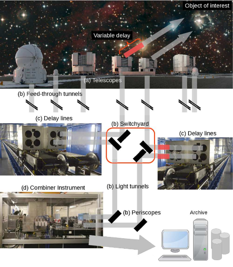
Figure 11: How to combine beams from separated telescopes illustrated with the vlti. The collected beams are first collimated and fed into tunnels by a set of mirrors in the telescopes, put into delay lines to compensate for the delay introduced by pointing and other effects (in red), then fed into the interferometric instruments that records the data.

7.3 Delay lines

Delay lines are a set of movable mirrors which compensate for the optical delay induced by the pointing of the telescope. These are supposedly simple at first glance but one needs to consider the required precision (less than 1$\mu$m), and range of motion (half the largest telescope baseline, i.e. it can be hundreds of meters). These optical systems are in no way simple to build and operate, as the mirrors-bearing carriage has to provide sub-micron position accuracy on hundreds of meters with a continuous motion of a few centimetres per second…

Several technical solutions have been implemented, which all have advantages and drawbacks: the delay lines can be in the air (like on vlti or Keck-I) or in vacuum (like on iota), or partially in vacuum and partially in air (like in chara, npoi). They can be one stage (vlti) or two stages (iota, Keck-I, chara, npoi) with a long-stroke fixed delay (easier to manufacture) and short-stroke moving delay.

7.4 Combiner

The last element of the interferometer is the Combiner. It is basically a Michelson or a Fizeau interferometer plugged-in to a very sophisticated video camera with some degree of spectral dispersion and a feedback loop to stabilise the fringes. The fringe combination can be done in different ways and we refer the reader to Berger ([2015], this book) for further details.

All these sub-systems are shown in the illustration Fig. 11.

8 Optical interferometry in 2015

8.1 vlti

The vlti is the only large-aperture interferometer in operation today. With its four 8-meter class telescopes, supplemented by four movable 2-meter class telescopes (see Fig 11), it offers versatility and sensitivity at the same time. It saw its first light in 2001 (Glindemann et al. [2001]) with the vinci instrument, and has since seen its capabilities increasing: 2 recombined telescopes in 2001 (Kervella et al. [2003]), mid-infrared with midi (Leinert et al. [2003]), 3 telescopes and a high spectral resolution in 2004 with amber (Petrov et al. [2007]) and 4 telescopes in 2010 with pionier (Le Bouquin et al. [2011], but lacking a high or medium spectral resolution, and just open to the general community since 2015). The vlti is noticeably the most productive interferometric facility in the world (see Fig. 12). Applying for observing time is open to any professional astronomer, and its archive is public after typically one year of ownership by the PI. The next generation instruments matisse and gravity will offer to the wide community four telescopes and, for the first time, real imaging capabilities.

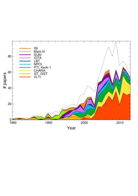
Figure 12: Publications related to long-baseline interferometry per year (Data from the JMMC http://apps.jmmc.fr/bibdb/). The dash line represent the total number of publication whereas the colors are per facility (i.e. observations papers only). We can see a steep increase after 2002 with the advent of vlti, and a decrease after 2010 due to the closure of several facilities (Keck-I, IOTA, …).

8.2 chara

chara is a six-1-meter-class telescopes interferometer, which is funded and operated by the Georgia State University. It has developed in the 2000s a collaborative framework allowing teams from all over the world to install and operate instruments on the facility. As a result, chara is the interferometer with the most number of currently-operated instruments, with classic, climb, mirc, pavo, vega. chara has the longest operating baselines (300 m) and works in the visible range, making it the sharpest telescope on Earth.

8.3 npoi

npoi is a six-telescope interferometer jointly operated by the Lowell Observatory and the US Navy. It consists of small apertures movables siderostats for imaging as well as fixed siderostats dedicated to astrometry. Its recent developments include a 6-telescope visible instrument vision and the commissioning of new longer baselines. It is currently limited by the small apertures, but the developement plan includes the installation of meter-class telescopes in the future.

8.4 The legacy

The long-term durability of the data acquired by the interferometers make it a goldmine for future astronomers. Therefore some observatories have made an effort to archive the obtained data and to make it public for future use. This is e.g. the case for the ESO science archive facility which provides raw datasets from all the open vlti instruments plus, more recently, data from the visitor instrument pionier.

Since ESO provides only raw datasets, a community effort is being made, led by JMMC, to provide a reduced database called OIDB. It will provide in a near-future reduced datasets which have been published, in order to make them accessible for future use.

An effort has also been conducted to make the legacy Keck-I and PTI instruments data avilable through the PTI & Keck Public Database. Future users can access freely these data and use them in a publication provided they follow the publishing guidelines available at ESO and NExScI webpages.

9 The future: new instruments, new possibilities

The vlti has been at the leading edge for optical interferometry in the last decade. However, the two first-generation instruments, amber and midi are now 10 years old, and even though they have unmatched features (high spectral resolution for amber and N band for midi), they start to show their limits. Therefore, ESO issued a call for proposals in 2005 to build second generation instruments. Two projects were selected: gravity, aiming at performing micro-arcseconds astrometry on the Galactic Center in the near-infrared, and matisse, aiming at opening the L band in addition to bring imaging capabilities to the vlti in the mid-infrared. They both come to the sky in the 5+ years from now.

The chara array is being fitted with adaptive optics to improve by a large factor its performances, especially at short wavelengths, offering new possibilities of performant instrumentation in the 5+ years to come.

In the meantime, several projects have emerged to pave the way of future facilities: a visible interferometry prospective is being conducted today (Stee et al. in prep.), to make emerge a new generation instrumentation at vlti and chara in the 10+ years; a more general prospective is conducted by the Europan Interferometry Initiative to direct future instruments in the same timeline (Pott, private communication); the Planet Formation Imager project (Kraus et al. [2014]) aims at imaging and characterizing an exoplanet in the 20+ coming years; finally several bold prototypes of completely new combination schemes (le Coroller et al. [2015], Labeyrie et al. [2001], and see also the conclusion of this book: Labeyrie [2015]), hypertelescopes, are being imagined, developed and tested to gather the technologies necessary for the 40+ years to come.

Acknowledgements: The author would like to thank R. Petrov, A. Meilland and G. Dalla Vedova for reading through this paper and for suggesting improvements. Thanks also to J.-F. Sauvage for interesting discussions about technical aspects on the VLT, and to J.-U. Pott for pushing the prospective on the future of interferometry.

References

- [1921] Michelson, A. A. & Pease, F. G. 1921, ApJ, 53, 249
- [1958] Jennison, R. C. 1958, MNRAS, 118, 276
- [1970] Labeyrie, A. 1970, A&A, 6, 85
- [1982] Beckers, J. M. 1982, Optica Acta, 29, 361
- [1984] Pearson, T. J. & Readhead, A. C. S. 1984, A&A Ann. Rev., 22, 97
- [1986] Aime, C.; Borgnino, J.; Martin, F. et al. 1986, J. Opt. Soc. Am. A, 3, 1001
- [1988] Pérez, J. P. 1988, Optique géométrique et ondulatoire, Masson
- [1992] Shao, M. & Colavita, M. M. 1992, A&A Ann. Rev., 30, 457
- [1994] Mourard, D.; Tallon-Bosc, I.; Rigal, F. et al. 1994, A&A, 288, 675
- [1999] Berger, J.-P., Schanen-Duport, I., El-Sabban, S., et al. 1999, in ASP Conf. Ser. 194, 264
- [1999] Born, M., Wolf, E. 1999, Principles of optics, Cambridge University Press
- [2000] Lawson, P. R. 2000, in Principles of Long Baseline Stellar Interferometry, ed. P. R. Lawson, 325
- [2001] Altarac, S., Berlioz-Arthaud, P., Thiébaut, E. et al. 2001, MNRAS, 322, 141
- [2001] Glindemann, A., Bauvir, B., Delplancke, F., et al. 2001, The Messenger, 104, 2
- [2001] Labeyrie, A. and Arnold, L. and Gillet, S. et al. 2001, SF2A, 505
- [2001] Merand, A.; ten Brummelaar, T.; McAlister, H. et al. AAS, 198, 6104
- [2002] Papoulis, A. and Pillai, S. U., 2002, Probability, Random Variables, and Stochastic Processes, McGraw-Hill Higher Education
- [2003] Arsenault, R. and Alonso, J. and Bonnet et al. 2003, The Messenger, 112, 7
- [2003] Hess, M., Nance, C. E., Vause, J. W., et al. 2003, SPIE, 4837, 342
- [2003] Kervella, P., Gitton, P. B., Segransan, D., et al. 2003, SPIE, 4838, 858
- [2003] Lachaume, R. 2003, A&A, 400, 795
- [2003] Leinert, C., Graser, U., Przygodda, F., et al. 2003, ApSS, 286, 73
- [2003] Monnier, J. D., Reports on Progress in Physics, 66, 789
- [2003a] Perrin, G. 2003a, A&A, 398, 385
- [2003b] Perrin, G. 2003b, A&A, 400, 1173
- [2004] Millour, F., Tatulli, E., Chelli, A. E., et al. 2004, SPIE, 5491, 1222
- [2004] Pauls, T. A., Young, J. S., Cotton, W. D., & Monnier, J. D. 2004, SPIE, 5491, 1231
- [2004] Tubbs, R. N., Meisner, J. A., Bakker, E. J., & Albrecht, S. 2004, SPIE, 5491, 588
- [2005] Pauls, T. A., Young, J. S., Cotton, W. D., & Monnier, J. D. 2005, Publications of the ASP, 117, 1255
- [2006] Lopez, B., Wolf, S. Lagarde, S. et al. 2006, SPIE, 6268, 31
- [2006] Millour, F.; Vannier, M.; Petrov et al. 2006, EAS Publications Series, 22, 379
- [2006] Millour, F. 2006, Interférométrie différentielle avec AMBER, PhD thesis, Univ. Joseph Fourier
- [2006] Monnet, G. & Gilmozzi, R. 2006, in IAU Symposium, Vol. 232, The Scientific Requirements for Extremely Large Telescopes, 429
- [2006] Monnier, J. D. and Berger, J.-P. and Millan-Gabet, R. et al. 2006, ApJ, 647, 444
- [2006] Vannier, M., Petrov, R. G., Lopez, B., & Millour, F. 2006, MNRAS, 367, 825
- [2007] Petrov, R. G., Malbet, F., Weigelt, G., et al. 2007, A&A, 464, 1
- [2007] Segransan, F. 2007, New Astronomy Review, 51, 597
- [2007] Tatulli, E., Millour, F., Chelli, A., et al. 2007, A&A, 464, 29
- [2007] Tristram, K. R. W.; Meisenheimer, K.; Jaffe, W. et al. 2007, A&A, 474, 837
- [2007] Weigelt, G. and Kraus, S. and Driebe, T. et al. 2007, A&A, 464, 87
- [2008] Köhler, R. and Jaffe, W., 2008 Power of Optical/IR Interferometry conf. 569
- [2008] Kraus, S. and Hofmann, K.-H. and Benisty et al. 2008, A&A, 489, 1157
- [2008] Millour, F. 2008, New Astronomy Review, 52, 177
- [2008] Millour, F., Petrov, R., Malbet, F., et al. 2008, in 2007 ESO Instrument Calibration Workshop, 461
- [2008] Tallon-Bosc, I.; Tallon, M.; Thiébaut, E. et al. 2008, SPIE, 7013
- [2009] Chelli, A., Duvert, G., Malbet, F., & Kern, P. 2009, A&A, 498, 321
- [2009] Demory, B. O., Ségransan, D., Forveille, T. 2009, A&A, 505, 205
- [2009] Haubois, X., Perrin, G., Lacour, S., et al. 2009, A&A, 508, 923
- [2009] Lombardi, G., Zitelli, V., & Ortolani, S. 2009, MNRAS, 399, 783
- [2009] Millour, F.; Chesneau, O.; Borges Fernandes et al. 2009, A&A507, 317
- [2009] Millour, F.; Driebe, T.; Chesneau, O. et al. 2009, A&A, 506, L49
- [2009] Mourard, D.; Clausse, J. M.; Marcotto et al., 2009, A&A, 508, 1073
- [2009] Schmitt, H. R., Pauls, T. A., Tycner, C., et al. 2009, ApJ, 691, 984
- [2010] Benisty, M. and Natta, A. and Isella et al. 2010, A&A, 511, A74
- [2010] Jankov, S. 2010, Serbian Astronomical Journal, 181, 1
- [2010] Lizon, J. L., Jakob, G., de Marneffe, B., & Preumont, A. 2010, SPIE, 7739
- [2010] Poupar, S., Haguenauer, P., Merand, A., et al. 2010, SPIE, 7734
- [2010] Spaleniak, I., Giessler, F., Geiss, R., et al. 2010, SPIE, 7734
- [2011] Chesneau, O., Meilland, A., Banerjee, D. P. K., et al. 2011, A&A, 534, L11
- [2011] Glindemann, A. 2011, Principles of Stellar Interferometry
- [2011] Kishimoto, M.; Hönig, S. F.; Antonucci, R. et al. 2011, A&A, 527, 121
- [2011] Le Bouquin, J.-B., Berger, J.-P., Lazareff, B., et al. 2011, A&A, 535, A67
- [2011] Meilland, A. and Delaa, O. and Stee, P. et al. 2011, A&A, 532, A80
- [2011] Millour, F., Meilland, A., Chesneau, O., et al. 2011, A&A, 526, A107
- [2011] Mourard, D., Bério, P., Perraut, K., et al. 2011, A&A, 531, A110
- [2011] Ohnaka, K., Weigelt, G., Millour, F., et al. 2011, A&A, 529, A163
- [2012] Stee, P. and Delaa, O. and Monnier, J. D. et al. 2012, A&A, 545, A59
- [2012] Lazareff, B., Le Bouquin, J.-B., & Berger, J.-P. 2012, A&A, 543, A31
- [2012] Meilland, A. and Millour, F. and Kanaan, S. et al. 2012, A&A, 538, A110
- [2012] Kloppenborg, B.; Baron, F. 2012, SIMTOI: SImulation and Modeling Tool for Optical Interferometry. Available from \urlhttps://github.com/bkloppenborg/simtoi
- [2013] Ohnaka, K., Hofmann, K.-H., Schertl, D., et al. 2013, A&A, 555, A24
- [2014] Defrère, D., Absil, O., Hanot, C., et al. 2014, in Improving the Performances of Current Optical Interferometers & Future Designs, 87
- [2014] Kraus, S. and Monnier, J. and Harries, T. et al. 2014, SPIE, 9146, 120
- [2014] Mourard, D., Monnier, J. D., Meilland, A., et al. 2015, A&A, 577,51
- [2014] Schutz, A.; Ferrari, A.; Mary et al. ArXiv e-prints, 2014
- [2014] Schutz, A.; Vannier, M.; Mary, D. et al. 2014, A&A, 565, A88
- [2014] Soulez, F. and Thiébaut, É. 2014, in Improving the Performances of Current Optical Interferometers & Future Designs 255
- [2014] Woillez, J., Perrin, G., Lai, O., et al. 2014, in Improving the Performances of Current Optical Interferometers & Future Designs, 175
- [2015] Berger, J.-P. 2015, this book
- [2015] Domiciano, A., 2015, this book
- [2015] Labeyrie, A. 2015, this book
- [2015] Le Coroller, H. and Dejonghe, J. and Hespeels, F. et al. 2015, A&A, 573, A117
- [2015] Lena, P. 2015, Some historical insights on optical interferometry, this book.
- [2015] ten Brummelaar, T. 2015, CLASSIC/CLIMB Theory, this book.
- [2015] Young, J. and Thiébaut, E. 2015, this book