Effects of Thermal Fluctuations on the Thermodynamics of Modified Hayward Black Hole

Abstract

In this work, we analyze the effects of thermal fluctuations on the thermodynamics of a modified Hayward black hole. These thermal fluctuations will produce correction terms for various thermodynamic quantities like entropy, pressure, inner energy and specific heats. We also investigate the effect of these correction terms on the first law of thermodynamics. Finally, we study the phase transition for the modified Hayward black hole. It is demonstrated that the modified Hayward black hole is stable even after the thermal fluctuations are taken into account, as long as the event horizon is larger than a certain critical value.

Keywords: Black hole; Thermodynamics.

1 Introduction

The black hole entropy obtained by famous formula $S=A/4$, where $A$ denotes the area of the event horizon [1]. This is the maximum entropy contained by any object of the same volume [2, 3]. It may be noted that a maximum entropy has to be associated with the black holes to prevent the violation of the second law of thermodynamics [4, 5]. The reason is that, if a black hole did not have any entropy, then the entropy of the universe would spontaneous reduce when any object crosses the horizon. The observation that the entropy of a black hole scales with its area has led to the development of the holographic principle [6, 7]. This principle equates the degrees of freedom in a region of space with the degrees of freedom on the boundary of that region.

Even though the holographic principle is expected to hold for large regions of space, it is expected to get violated near the Planck scale [8, 9]. This violation of the holographic principle occurs due to the quantum fluctuations in the geometry of space-time. As these quantum fluctuations are expected to dominate the geometry of space-time near the Planck scale, it is expected that the holographic principle will be violated near the Planck scale. Thus, the relation between the area and entropy of a black hole is also expected to get modified near the Planck scale. In fact, the quantum fluctuations in the geometry of the black hole will lead to the thermal fluctuations in the black hole thermodynamics [10, 11]. It will be possible to neglect these thermal fluctuations for the large black holes. However, as the black holes reduce in size due to the radiation of the Hawking radiation, the quantum fluctuations in the geometry of the black hole will increase. Thus, the thermal fluctuations will start to modify the thermodynamics of the black holes as the black holes reduce in size. It is possible to calculate the correction terms generated from such thermal fluctuations. The correction terms generated from these thermal fluctuations are logarithmic functions of the original thermodynamic quantities.

The corrections to the black hole thermodynamics have been obtained using the density of microstates for asymptotically flat black holes [12]. This was done by using a formalism called the non-perturbative quantum general relativity. In this formalism, the density of states for a black hole was associated with the conformal blocks of a well defined conformal field theory. It was demonstrated that even though the leading order relation between the entropy and area of a black hole is the standard Bekenstein entropy-area relation, this formalism also generated logarithmic corrections terms to the standard Bekenstein entropy-area relation. It has also been demonstrated using the Cardy formula that the logarithmic correction terms are generated for all black holes whose microscopic degrees of freedom are described by a conformal field theory [13]. Matter fields have been studied in the presence of a black hole, and this analysis has also generated logarithmic correction terms for the Bekenstein entropy-area formula [14, 15, 16]. The logarithmic correction terms are also generated from string theoretical effects [17, 18, 19, 20]. The corrections term for the entropy of a dilatonic black holes has been calculated [21]. It was found that this correction term is again a logarithmic functions of the original thermodynamic quantities. Such correction terms have also been generated using a Rademacher expansion of the partition function [22]. So, it seems that such logarithmic corrections terms occur almost universally.

The singularity at the center of black holes indicates a breakdown of general theory of relativity, as it cannot be gauged away by coordinate transformations. However, it is possible to construct black holes which are regular and do not contain an singularity at the center. The Hayward black hole is an example of such regular black hole as it does not contain a singularity at the center [23, 24]. These black holes have been analyzed using various modifications of the Chaplygin gas formalism [25, 26, 27, 28, 29, 30, 31]. The motion of a particle in background of a Hayward black hole also has been discussed [32]. The massive scalar quasinormal modes of the Hayward black hole have been studied [33]. In fact, the one-loop quantum corrections to the Newton potential for these regular black holes has been calculated in [34]. Recently, the accretion of fluid flow around the modified Hayward black hole have been analyzed [35]. The acceleration of particles in presence of a rotating modified Hayward black hole has also been investigated [36]. In this paper, we will analyze the effects of thermal fluctuations on thermodynamics of a modified Hayward black hole.

2 Modified Hayward Black Hole

The most general spherically symmetric, static line element describing modified Hayward black hole can be written as [34, 35],

$$ds^{2}=-f(r)B(r)dt^{2}+\frac{dr^{2}}{B(r)}+r^{2}d\Omega^{2},$$ (1)

where

$$d\Omega^{2}=d\theta^{2}+\sin^{2}\theta d\phi^{2},$$ (2)

with

$$B(r) = 1-\frac{2Mr^{2}}{r^{3}+2Ml^{2}},$$

$$f(r) = 1-\frac{\alpha\beta M}{\alpha r^{3}+\beta M},$$ (3)

where $M$ is the black hole mass, $l$ is the Hubble length which is related to the cosmological constant, $\alpha$ is a positive constants and $\beta$ is related with the cosmological constant [37]. In the Ref. [35] it is found that $\alpha>1$. We will find lower bounds for both $\alpha$ and $\beta$ using the thermodynamics description.
The horizon radius of the black hole can be found by the real positive root of the following equation,

$$r_{+}^{3}-2Mr_{+}^{2}+2Ml^{2}=0.$$ (4)

So, one can obtain the black hole mass in terms of the horizon radius as follows,

$$M=\frac{r_{+}^{3}}{2(r_{+}^{2}-l^{2})},$$ (5)

which implies that $r_{+}^{2}>l^{2}$. For simplicity we set $l=1$. Then, the equation (4) has a solution as follow,

$$r_{+}=\frac{X}{3}+\frac{4M^{2}}{3X}+\frac{2}{3}M,$$ (6)

where,

$$X\equiv\left(8M^{3}-27M+3\sqrt{81M^{2}-48M^{4}}\right)^{\frac{1}{3}},$$ (7)

which gives an upper bound for the black hole mass,

$$M\leq\frac{3\sqrt{3}}{4}.$$ (8)

For the special case of $M=\frac{3\sqrt{3}}{4}$, where $X=2M$, the event horizon radius reduces to $r_{+}=2M=\frac{3\sqrt{3}}{2}$.
An important thermodynamic quantity is the entropy which is related to the black hole horizon area,

$$S_{0}=\pi r_{+}^{2}$$ (9)

Also, volume of the black hole is given by,

$$V=\frac{4}{3}\pi r_{+}^{3}.$$ (10)

Temperature of modified Hayward black hole can be written as,

$$T=\left[\frac{1}{4\pi}\sqrt{-g^{tt}g^{rr}}~{}\frac{d}{dr}g_{tt}\right]_{r=r_{+}}=\frac{1}{4\pi}\frac{r_{+}^{3}-4M}{2Mr_{+}^{3}}\sqrt{1-\frac{\alpha\beta M}{\alpha r_{+}^{3}+\beta M}},$$ (11)

where the black hole mass $M$ is given by the equation (5) and black hole horizon radius is given by the equation (6). Therefore, we can investigate thermodynamics of black hole in terms of either black hole mass or radius associated with the event horizon. Now, the temperature of the black hole can be simplified to the another form,

$$T=\frac{r_{+}^{2}-3}{4\pi r_{+}^{3}}\sqrt{\frac{2\alpha r_{+}^{2}-\alpha\beta-2\alpha+\beta}{2\alpha r_{+}^{2}-2\alpha+\beta}}.$$ (12)

There are two conditions to have real positive temperature,

$$r_{+}^{2} \geq 3,$$

$$r_{+}^{2} \geq \frac{\alpha\beta+2\alpha-\beta}{2\alpha}.$$ (13)

Both conditions satisfied simultaneously if we have,

$$\beta(1-\frac{1}{\alpha})\geq 4.$$ (14)

It shows that $\alpha>1$ is necessary to have positive $\beta$, as illustrated by Ref. [35]. If we assume integer values for $\alpha$ and $\beta$, quickly we find $\beta\geq 8$. Therefore, $\alpha=2$ and $\beta=8$ are corresponding to the zero-temperature limit, and both conditions of (2) are the same. The case of $\beta=0$ yields to ordinary Hayward black hole [23] with the temperature given by,

$$T=\frac{r_{+}^{2}-3}{4\pi r_{+}^{3}},$$ (15)

which reduces to $T=1/4\pi r_{+}$ for the large values of horizon radius (asymptotic behavior). The pressure can be obtained by

$$P=\frac{T}{2r_{+}}.$$ (16)

It is interesting to investigate the first law of thermodynamic [38, 39],

$$dM=TdS+VdP+...,$$ (17)

other terms are corresponding to the black hole rotation and charge which are absent in our model. It is easy to check that the equation (17) violates. In order for thermodynamic quantities satisfy above relation, we have two solutions: the first is to add rotation or charge to the black hole, the second is consideration of logarithmic correction.

3 Logarithmic correction

It is possible to calculate the effect of thermal fluctuations on the thermodynamics of modified Hayward black hole. One can write the partition function of the system as

$$Z=\int DgDAe^{-I},$$ (18)

where $I\to-iI$ is the Euclidean action for this system [40]. It is possible to relate it to the partition function in the statistical mechanical as

$$Z=\int_{0}^{\infty}dE\,\,\rho(E)e^{-\beta_{\kappa}E},$$ (19)

where $\beta_{\kappa}$ is the inverse of the temperature. The partition function can be used to calculate the density of states

$$\rho(E)=\frac{1}{2\pi i}\int^{\beta_{0\kappa}+i\infty}_{\beta_{0\kappa}-i\infty}d\beta_{\kappa}\,\,e^{S(\beta_{\kappa})},$$ (20)

where

$$S=\beta_{\kappa}E+\ln Z.$$ (21)

The entropy around the equilibrium temperature $\beta_{0\kappa}$ can be obtained by neglecting all the thermal fluctuations. However, if thermal fluctuations are taken into account, then $S(\beta_{\kappa})$, can be written as

$$S=S_{0}+\frac{1}{2}(\beta_{\kappa}-\beta_{0\kappa})^{2}\left(\frac{\partial^{2}S(\beta_{\kappa})}{\partial\beta_{\kappa}^{2}}\right)_{\beta_{\kappa}=\beta_{0\kappa}}.$$ (22)

So, the density of states can be written as

$$\rho(E)=\frac{e^{S_{0}}}{2\pi i}\int^{\beta_{0\kappa}+i\infty}_{\beta_{0\kappa}-i\infty}d\beta_{\kappa}\,\,\exp\left(\frac{1}{2}(\beta_{\kappa}-\beta_{0\kappa})^{2}\left(\frac{\partial^{2}S(\beta_{\kappa})}{\partial\beta_{\kappa}^{2}}\right)_{\beta_{\kappa}=\beta_{0\kappa}}\right).$$ (23)

Thus, we obtain

$$\rho(E)=\frac{e^{S_{0}}}{\sqrt{2\pi}}\left[\left(\frac{\partial^{2}S(\beta_{\kappa})}{\partial\beta_{\kappa}^{2}}\right)_{\beta_{\kappa}=\beta_{0\kappa}}\right]^{1/2}.$$ (24)

So, we can write

$$S=S_{0}-\frac{1}{2}\ln\left[\left(\frac{\partial^{2}S(\beta_{\kappa})}{\partial\beta_{\kappa}^{2}}\right)_{\beta_{\kappa}=\beta_{0\kappa}}\right]^{1/2}.$$ (25)

This expression can be simplified using the relation between the microscopic degrees of freedom of a black hole and a conformal field theory. This is because using this relation, the entropy can be assumed to the form, $S=a_{1}\beta_{\kappa}^{m}+a_{2}\beta_{\kappa}^{-n}$, where $a_{1},a_{2},m,n$ are positive constants [13]. This has an extremum at $\beta_{0\kappa}=(na_{2}/ma_{1})^{1/m+n}=T^{-1}$ and so we can expand the entropy around this extremum

$$S(\beta_{\kappa}) = [(n/m)^{m/(m+n)}+(m/n)^{n/(m+n)}](a_{1}^{n}a_{2}^{m})^{1/(m+n)}$$ (26)

$$+\frac{1}{2}[(m+n)m^{(n+2)/(m+n)}n^{(m-2)/(m+n)}](a_{1}^{n+2}a_{2}^{m-2})^{{1}/(m+n)}$$

$$\times(\beta_{\kappa}-\beta_{0\kappa})^{2},$$

Now we can write

$$S_{0} = (n/m)^{m/(m+n)}+(m/n)^{n/(m+n)}(a_{1}^{n}a_{2}^{m})^{{1}/(m+n)},$$

$$\left(\frac{\partial^{2}S(\beta_{\kappa})}{\partial\beta_{\kappa}^{2}}\right)_{\beta_{\kappa}=\beta_{0\kappa}} = (m+n)m^{(n+2)/(m+n)}n^{(m-2)/(m+n)}$$ (27)

$$\times(a_{1}^{n+2}a_{2}^{m-2})^{1/(m+n)}~{}~{}.$$

It is possible to solve for $a_{1},a_{2}$ and express the entropy as

$$\left(\frac{\partial^{2}S(\beta_{\kappa})}{\partial\beta_{\kappa}^{2}}\right)_{\beta_{\kappa}=\beta_{0\kappa}}=\mathcal{Y}S_{0}T^{2}~{},$$ (28)

where

$$\mathcal{Y} = \left[\left(\frac{(m+n)m^{(n+2)/(m+n)}n^{(m-2)/(m+n)}}{(n/m)^{m/(m+n)}+(m/n)^{n/(m+n)}}\right)~{}\right.$$ (29)

$$\left.\times\left(\frac{n}{m}\right)^{2/(m+n)}\right].$$

However, the factor $\mathcal{Y}$ can be absorbed using some redefinition as it does not depend on the black hole parameters [10, 11]. Thus, we can write

$$\left(\frac{\partial^{2}S(\beta_{\kappa})}{\partial\beta_{\kappa}^{2}}\right)_{\beta_{\kappa}=\beta_{0\kappa}}=S_{0}\beta_{0\kappa}^{-2}.$$ (30)

So, the corrected value of the entropy can be written as

$$S=S_{0}-\frac{1}{2}\ln{S_{0}T^{2}},$$ (31)

We can write a general expression for the entropy as

$$S=S_{0}-\frac{b}{2}\ln{S_{0}T^{2}},$$ (32)

where we introduced a parameter $b$ by hand to track corrected terms, so in the limit $b\rightarrow 0$, the original results can be recovered and $b=1$ yields usual corrections [11]. By using the temperature and entropy given by the equations (11) and (9) respectively, we can obtain the following corrected entropy,

$$S=\pi r_{+}^{2}-\frac{b}{2}\ln\left[\frac{(r_{+}^{2}-3)^{2}(2\alpha r_{+}^{2}-\alpha\beta-2\alpha+\beta)}{16\pi r_{+}^{4}(2\alpha r_{+}^{2}-2\alpha+\beta)}\right].$$ (33)

It is clear that the logarithmic correction reduce the entropy of the black hole. We can obtain the entropy at zero-temperature using appropriate choice of $\alpha$ and $\beta$ ($\alpha=2$ and $\beta=8$),

$$S(T=0)=\pi r_{+}^{2}-\frac{b}{2}\ln\sqrt{\frac{(r_{+}^{2}-3)^{3}}{16\pi r_{+}^{4}(r_{+}^{2}+1)}}.$$ (34)

As we mentioned already, both zero-temperature conditions (2) are the same for $\alpha=2$ and $\beta=8$. So, $r_{+}=\sqrt{3}$ is zero-temperature condition where entropy (34) become infinite. The fact is that at the zero-temperature limit, thermal fluctuations vanish and we should set $b=0$. It is clear from the equation (32), so at the zero-temperature limit we have $S(T=0)=3\pi$.
We can calculate pressure using the (9), (10), (11) and following relation,

$$P=T\left(\frac{\partial S}{\partial V}\right)_{V}.$$ (35)

In the Fig. 1, we can analyze the behavior of pressure for various values of parameters. Comparing dashed line and dotted line, we can find that the logarithmic correction decrease the pressure. Using the higher values for the black hole mass from the relation (8), we find zero pressure around the black hole horizon. Higher values of the mass yields to negative pressure. For all cases with $M<\frac{3\sqrt{3}}{4}$, we can see positive pressure, which yields to zero as $M\rightarrow 0$, it is clearly expected that vanished black hole has no thermodynamics pressure.

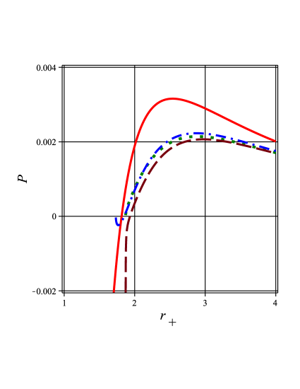
Figure 1: Pressure versus horizon radius with $\alpha=2$. $b=1$, $\beta=10$ (dashed line); $b=1$, $\beta=0$ (solid line); $b=0$, $\beta=10$ (dotted line); $b=1$, $\beta=8$ (dash dotted line).

Then, using the well known relation,

$$E=\int{TdS},$$ (36)

we can obtain inner energy which decreased dramatically due to the logarithmic corrections. It may be noted that $T$ and $S$ can be used to obtain the specific heat at constant volume,

$$C_{v}=\left(T\frac{\partial S}{\partial T}\right)_{V}.$$ (37)

Calculation of $P$ and $E$ help us to obtain specific heat at constant pressure,

$$C_{p}=\left(\frac{\partial(E+PV)}{\partial T}\right)_{P}.$$ (38)

So, we can investigate $\gamma=C_{p}/C_{v}$ numerically. From the Fig. 2 it is illustrated that, for the large horizon radius, $\gamma\rightarrow 0.5$. We find that the value of $\gamma$ increased due to the logarithmic corrected entropy.

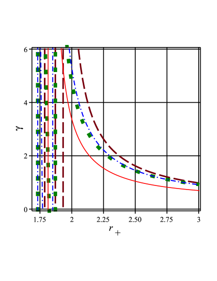
Figure 2: $\gamma$ in terms of horizon radius with $\alpha=2$. $b=1$, $\beta=10$ (dashed line); $b=1$, $\beta=0$ (solid line); $b=0$, $\beta=10$ (dotted line); $b=1$, $\beta=8$ (dash dotted line).

Now, in order to investigate the first law of thermodynamic we rewrite the equation (17) as follow,

$$X=Y,$$ (39)

where $X\equiv dM-TdS$ and $Y\equiv VdP$. Then, we give plots of $X$ and $Y$ in terms of the radius of a black hole horizon in Fig. 3. We draw three curves corresponding to each $X(\alpha,\beta)$ and $Y(\alpha,\beta)$. We see that, at least, there are two points where the first law of thermodynamic is satisfied. Cross points of the red (solid) and blue (dashed) curves states $X=Y$ which means validity of the relation (17). Therefore, we can say that, the first law of thermodynamic may also valid for the modified Hayward black hole. There are some special cases with suitable horizon radius where the first law of thermodynamics is satisfied.

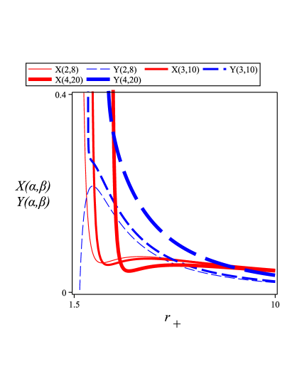
Figure 3: X (solid red) and $Y$ (dashed blue) in terms of $r_{+}$ with $b=1$ for various values of $\alpha=2,3,4$ and $\beta=8,10,20$.

4 Phase transition

One of the best ways to find instability of a black hole is studied the sign of the specific heat given by the equation (37). The black hole is stable for $C_{v}>0$, while is unstable for $C_{v}<0$. Therefore, $C_{v}=0$ show the point of phase transition. It is easy to write the specific heat at constant volume as follow,

$$C_{v}=\frac{A_{1}r_{+}^{8}+A_{2}r_{+}^{6}+A_{3}r_{+}^{4}+A_{4}r_{+}^{2}+A_{5}}{A_{6}r_{+}^{6}+A_{7}r_{+}^{4}+A_{8}r_{+}^{2}+A_{9}},$$ (40)

where,

$$A_{1} = 8\pi\alpha^{2},$$

$$A_{2} = 4\pi\alpha(2\beta-10\alpha-\alpha\beta),$$

$$A_{3} = 16\pi\beta\alpha^{2}-2\pi\alpha\beta^{2}-2b\beta\alpha^{2}+56\pi\alpha^{2}-32\pi\alpha\beta+2\pi\beta^{2}-24b\alpha^{2},$$

$$A_{4} = 6\pi\alpha\beta^{2}-12\pi\beta\alpha^{2}+18b\beta\alpha^{2}-24\pi\alpha^{2}+24\pi\alpha\beta-6\pi\beta^{2}+48b\alpha^{2}-24b\alpha\beta,$$

$$A_{5} = 6b\alpha\beta^{2}-12b\beta\alpha^{2}-24b\alpha^{2}+24b\alpha\beta-6b\beta^{2},$$

$$A_{6} = -4\alpha^{2},$$

$$A_{7} = 4\alpha(\alpha\beta+11\alpha-\beta),$$

$$A_{8} = \alpha\beta^{2}-26\beta\alpha^{2}-76\alpha^{2}+40\alpha\beta-\beta^{2},$$

$$A_{9} = 18\beta\alpha^{2}-9\alpha\beta^{2}+36\alpha^{2}-36\alpha\beta+9\beta^{2}.$$ (41)

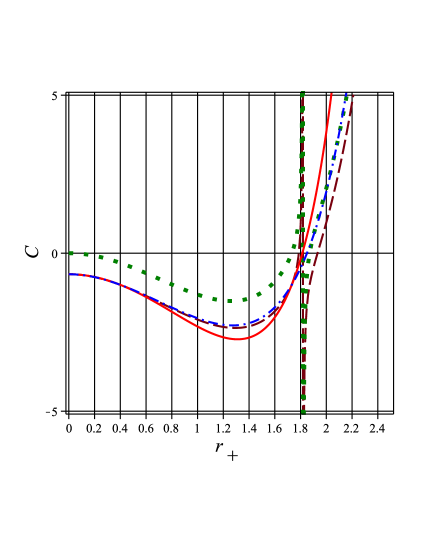
Figure 4: Specific heat at constant volume in terms of horizon radius with $\alpha=2$. $b=1$, $\beta=10$ (dashed line); $b=1$, $\beta=0$ (solid line); $b=0$, $\beta=10$ (dotted line); $b=1$, $\beta=8$ (dash dotted line).

We give graphical analysis of the specific heat which illustrated in Fig. 4. We can demonstrate that various cases of the black hole may be stable for the case of $r_{+}\geq\sqrt{3}$. It is clear that the modified Hayward black hole with logarithmic correction of entropy is stable for $r_{+}\geq 1.9$. Therefore, we can say that the modified Hayward black hole is stable for $r_{+}\geq r_{c}$, where $r_{c}$ is critical value (minimum value) for the radius of the event horizon. It may be related to the minimum mass required for the formation of the Hayward black hole [41]. At the zero-temperature limit, where logarithmic correction vanishes we have $r_{+}=r_{c}=\sqrt{3}$

5 Conclusions

In this work, we have studied the spherically symmetric, static modified Hayward black hole. The entropy, temperature and pressure have been calculated and found some restrictions on the parameters $\alpha$ and $\beta$. Next, we have analyzed the effects of thermal fluctuations on the thermodynamics of a Hayward black hole. Using the zero-temperature limit of the black hole, we have obtained the bounds $\alpha\geq 2$ and $\beta\geq 8$. Here, the equality holds only in the zero-temperature limit. We have also analyzed the logarithmic correction to entropy and obtained the behaviors of the pressure and specific heats numerically. We found that the value of the pressure and inner energy reduced due to these logarithmic corrections. We also studied phase transition for the modified Hayward black hole, and obtained critical point for such a phase transition. We also demonstrated that the first law of thermodynamics is satisfied for the modified Hayward black hole, even in presence of thermal fluctuations. It may be noted that the thermodynamics of black holes also gets modified because of the generalized uncertainty principle [42, 43]. Such correction terms are non-trivial, and can lead to interesting consequences like the existence of black hole remnants. It would be interesting to analyze the corrections to the thermodynamics of a regular Hayward black hole from the generalized uncertainty principle.

References

- [1] N. Altamirano, D. Kubiznak, R. B. Mann, and Z. Sherkatghanad, Galaxies 2, 89 (2014)
- [2] J. D. Bekenstein, Phys. Rev. D 7 , 2333 (1973)
- [3] J. D. Bekenstein, Phys. Rev. D 9, 3292 (1974)
- [4] ] S. W. Hawking, Nature 248, 30 (1974)
- [5] S. W. Hawking, Commun. Math. Phys. 43, 199 (1975)
- [6] L. Susskind, J. Math. Phys. 36, 6377 (1995)
- [7] R. Bousso, Rev. Mod. Phys. 74, 825 (2002)
- [8] D. Bak and S. J. Rey, Class. Quant. Grav. 17, L1 (2000)
- [9] S. K. Rama, Phys. Lett. B 457, 268 (1999)
- [10] S. Das, P. Majumdar and R. K. Bhaduri, Class. Quant. Grav. 19, 2355 (2002)
- [11] J. Sadeghi, B. Pourhassan, and F. Rahimi, Can. J. Phys. 92 (2014) 1638
- [12] A. Ashtekar, Lectures on Non-perturbative Canonical Gravity, World Scientific (1991)
- [13] T. R. Govindarajan, R. K. Kaul, V. Suneeta, Class. Quant. Grav. 18, 2877 (2001)
- [14] R. B. Mann and S. N. Solodukhin, Nucl. Phys. B523, 293 (1998)
- [15] A. J. M. Medved and G. Kunstatter, Phys. Rev. D60, 104029 (1999)
- [16] A. J. M. Medved and G. Kunstatter, Phys. Rev. D63, 104005 (2001)
- [17] S. N. Solodukhin, Phys. Rev. D57, 2410 (1998)
- [18] A. Sen, JHEP 04, 156 (2013)
- [19] A. Sen, Entropy 13, 1305 (2011)
- [20] D. A. Lowe and S. Roy, Phys. Rev. D82, 063508 (2010)
- [21] J. Jing and M. L Yan, Phys. Rev. D63, 24003 (2001)
- [22] D. Birmingham and S. Sen, Phys. Rev. D63, 47501 (2001)
- [23] S.A. Hayward, Phys. Rev. Lett. 96 (2006) 031103
- [24] M. Halilsoy, A. Ovgun, S.H. Mazharimousavi, Eur. Phys. J. C 74 (2014) 2796
- [25] A. Sen, Phys. Scr. T117 (2005) 70
- [26] L. Xu, J. Lu, Y. Wang, Eur. Phys. J. C 72 (2012) 1883
- [27] U. Debnath, A. Banerjee, S. Chakraborty, Class. Quant. Grav. 21 (2004) 5609
- [28] E.O. Kahya, B. Pourhassan, Astrophys. Space Sci. 353 (2014) 677
- [29] B. Pourhassan, E.O. Kahya, Results Phys. 4 (2014) 101
- [30] B. Pourhassan and E. O. Kahya, Advances in High Energy Physics 2014 (2014) 231452
- [31] E.O. Kahya, M. Khurshudyan, B. Pourhassan, R. Myrzakulov, A. Pasqua, Eur. Phys. J. C 75 (2015) 43
- [32] G. Abbas, U. Sabiullah, Astrophys. Space Sci. 352 (2014) 769
- [33] K. Lin, J. Li and S. Yang, Int. J. Theor. Phys. 52 (2013) 3771
- [34] T. De Lorenzo, C. Pacilioy, C. Rovelli and S. Speziale, Gen. Rel. Grav. 47 (2015) 41
- [35] U. Debnath, Eur. Phys. J. C75 (2015) 3, 129
- [36] B. Pourhassan and U. Debnath, [arXiv:1506.03443 [gr-qc]]
- [37] J. Li, H. Ma, K. Lin, Phys. Rev. D 88 (2013) 064001
- [38] J. Sadeghi, K. Jafarzade, B. Pourhassan, Int. J. Theor. Phys. 51 (2012) 3891
- [39] B. P. Dolan, Class. Quant. Grav. 28 (2011) 235017
- [40] B. Pourhassan and Mir Faizal, Europhys. Lett. 111: 40006, 2015
- [41] R. Tharanath, J. Suresh, V.C. Kuriakose, Gen. Rel. Grav. 47 (2015) 46
- [42] M. Faizal and M. Khalil, Int.J.Mod.Phys. A30 (2015) 1550144
- [43] A. F. Ali, JHEP 1209, 067 (2012)