Regge spectra of excited mesons, harmonic confinement and QCD vacuum structure

Abstract

An approach to QCD vacuum as a medium describable in terms of statistical ensemble of almost everywhere homogeneous Abelian (anti-)self-dual gluon fields is briefly reviewed. These fields play the role of the confining medium for color charged fields as well as underline the mechanism of realization of chiral $SU_{\rm L}(N_{f})\times SU_{\rm R}(N_{f})$ and $U_{A}(1)$ symmetries. Hadronization formalism based on this ensemble leads to manifestly defined quantum effective meson action. Strong, electromagnetic and weak interactions of mesons are represented in the action in terms of nonlocal $n$-point interaction vertices given by the quark-gluon loops averaged over the background ensemble. New systematic results for the mass spectrum and decay constants of radially excited light, heavy-light mesons and heavy quarkonia are presented. Interrelation between the present approach, models based on ideas of soft wall AdS/QCD, light front holographic QCD, and the picture of harmonic confinement is outlined.

I Introduction

Almost forty five years ago Feynman, Kislinger, and Ravndal noticed Feynman that the Regge spectrum of meson and baryon masses could be universally described by assuming the four-dimensional harmonic oscillator potential acting between quarks and antiquarks. During subsequent years the idea of four-dimensional harmonic oscillator re-entered the discussion about quark confinement several times in various ways. Leutwyler and Stern developed the formalism devoted to the covariant description of bilocal meson-like fields $\Phi(x,z)$ combined with the idea of harmonic confinement Leutwyler:1977vz ; Leutwyler:1977vy ; Leutwyler:1977pv ; Leutwyler:1977cs ; Leutwyler:1978uk . Considerations of paper Feynman and Leutwyler-Stern formalism Leutwyler:1977vz ; Leutwyler:1977vy ; Leutwyler:1977pv ; Leutwyler:1977cs ; Leutwyler:1978uk can be seen as the forerunners to at present time very popular soft wall AdS/QCD models Karch:2006pv and the light front holographic QCD deTeramond:2005su ; Brodsky:2006uqa ; deTeramond:2008ht . In recent years, the approaches to confinement based on the ideas of soft wall AdS/QCD model and light front holography demonstrated an impressive phenomenological success Karch:2006pv ; deTeramond:2005su ; Brodsky:2006uqa ; deTeramond:2008ht ; Swarnkar ; Gutsche:2015xva . The crucial for phenomenology features of these approaches are the particular dilaton profile $\varphi(z)=\kappa^{2}z^{2}$ and the harmonic oscillator form of the confining potential as the function of fifth coordinate $z$. All these approaches begin with different motivation but finally come to the Schrödinger type differential equation with the harmonic potential in $z$ defining the wave functions and mass spectrum of mesons and baryons.

The physical origin of the above-mentioned particular form of dilaton profile in AdS/QCD and light front holography as well as the harmonic potential in the Stern-Leutwyler studies and, hence, the Laguerre polynomial form of the meson wave functions, could not be identified within these approaches themselves. The preferable form of the dilaton profile and/or the potential are determined by the phenomenological requirement of Regge character of the excited meson mass spectrum Karch:2006pv ; Feynman ; Leutwyler:1977vz ; Leutwyler:1977vy ; Leutwyler:1977pv ; Leutwyler:1977cs ; Leutwyler:1978uk .

The approach presented in this paper has been developed in essence twenty years ago EN1 . It clearly incorporates the idea of harmonic confinement both in terms of elementary color charged fields and the composite colorless hadron field. The distinctive feature of the present approach is that it basically links the concept of harmonic confinement and Regge character of hadron mass spectrum to the specific class of nonperturbative gluon configurations – almost everywhere homogeneous Abelian (anti-)self-dual gluon fields. A posteriori a close interrelation of the Abelian (anti-)self-dual fields and the hadronization based on harmonic confinement can be read off the papers Leutwyler1 ; Leutwyler2 ; Minkowski ; Leutwyler:1977vz ; Leutwyler:1977vy ; Leutwyler:1977pv ; Leutwyler:1977cs ; Leutwyler:1978uk . In brief, the line of arguments is as follows (for more detailed exposition see NV ).

An important benchmark has been the observation of Pagels and Tomboulis Pagels that Abelian self-dual fields describe a medium infinitely stiff to small gauge field fluctuations, i.e. the wave solutions for the effective quantum equations of motion are absent. This feature was interpreted as suggestive of confinement of color. Strong argumentation in favour of the Abelian (anti-)self-dual homogeneous field as a candidate for the global nontrivial minimum of the effective action originates from the papers Minkowski ; Leutwyler2 ; NG2011 ; Pawlowski ; George:2012sb . In particular, Leutwyler has shown that the constant gauge field is stable (tachyon free) against small quantum fluctuations only if it is Abelian (anti-)self-dual covariantly constant field Minkowski ; Leutwyler2 . Nonperturbative calculation of the effective potential within the functional renormalization group Pawlowski supported the earlier one-loop results on existence of the nontrivial minimum of the effective action for the Abelian (anti-)self-dual field.

The eigenvalues of the Dirac and Klein-Gordon operators in the presence of Abelian self-dual field are purely discrete, and the corresponding eigenfunctions of quarks and gluons are of the bound state type. This is a consequence of the fact that these operators contain the four-dimensional harmonic oscillator, acting as a confining harmonic potential. Eigenmodes of the color charged fields have no (quasi-)particle interpretation but describe field fluctuations decaying in space and time. The consequence of this property is that the momentum representation of the translation invariant part of the propagator of the color charged field in the background of (anti-)self-dual Abelian gauge field is entire analytical function. The absence of pole in the propagator was treated as the absence of the particle interpretation of the charged field Leutwyler1 . However just the absence of a single quark or anti-quark in the spectrum can not be considered as sufficient condition for confinement. One has to explain the most peculiar feature of QCD – the Regge character of the physical spectrum of colorless hadrons. Usually Regge spectrum is related to the string picture of confinement, justified in two complementary ways and limits: classical relativistic rotating string connecting massless quark and antiquark, and the linear potential between nonrelativistic heavy quark and antiquark with the area law for the temporal Wilson loop as a relevant criterion for static quark confinement. Neither the homogeneous Abelian (anti-)self-dual field itself nor the form of gluon propagator in the presence of this background had the clue to linear quark-antiquark potential. Nevertheless, the analytic structure of the gluon and quark propagators and assumption about the randomness of the background field ensemble led both to the area law for static quarks and the Regge spectrum for light hadrons.

Randomness of the ensemble of almost everywhere homogeneous Abelian (anti-)self-dual gluon fields has been taken into account implicitly in the model of hadronization developed in EN1 ; EN via averaging of the quark loops over the parameters of the random fields. The nonlocal quark-meson vertices with the complete set of meson quantum numbers were determined in this model by the form of the color charged gluon propagator. The spectrum of mesons displayed the Regge character both with respect to total angular momentum and radial quantum number of the meson. The reason for confinement of a single quark and Regge spectrum of mesons turned out to be the same – the analytic properties of quark and gluon propagators.

This result has almost completed the quark confinement picture based on the random almost everywhere homogeneous Abelian (anti-)self-dual fields. Self-duality of the fields plays the crucial role in this picture. This random field ensemble represents a medium where the color charged elementary excitations exist as quickly decaying in space and time field fluctuations but the collective colorless excitations (mesons) can propagate as plain waves (particles). It should be stressed that in this formalism any meson looks much more like a complicated collective excitation of a medium (QCD vacuum) involving quark, antiquark and gluon fields than a nonrelativistic quantum mechanical bound state of charged particles (quark and anti-quark) due to some potential interaction between them. Within this relativistic quantum field description the Regge spectrum of color neutral collective modes appeared as a ”medium effect” as well as the suppression (confinement) of a color charged elementary modes.

However, besides this dynamical color charge confinement, a correct complete picture must include the limit of static quark-antiquark pair with the area law for the temporal Wilson loop. In order to explore this aspect an explicit construction of the random domain ensemble was suggested in paper NK1 , and the area law for the Wilson loop was demonstrated by the explicit calculation. Randomness of the ensemble (in line with Olesen7 ) and (anti-)self-duality of the fields are crucial for this result.

In this paper we briefly review the approach to confinement, chiral symmetry realization and bosonization based on the representation of QCD vacuum in terms of the statistical ensemble of almost everywhere homogeneous Abelian (anti-)self-dual gluon fields, systematically calculate the spectrum of radial meson excitations and their decay constants and outline the possible relation between the formalism of soft wall AdS/QCD and light-front holography, and this, at first sight, different approach.

The character of meson wave functions in hadronization approach EN1 is fixed by the form of the gluon propagator in the background of the specific class of vacuum gluon configurations. These wave functions are almost identical to the wave functions of the soft wall AdS/QCD with quadratic dilaton profile and Leutwyler-Stern formalism. In all three cases we are dealing with the generalized Laguerre polynomials as the functions of $z$. In the hadronization approach of EN1 and EN the fifth coordinate $z$ appears as the relative distance between quark and antiquark in the center of quark mass coordinate system, while the center of mass coordinate $x$ represents the space-time point where the meson field is localized. This treatment of coordinates goes in line with the Leutwyler-Stern approach. Comparison of the soft wall AdS/QCD action and the effective action for auxiliary bilocal meson-like fields of the hadronization approach hints at the link between very appearance of dilaton and its particular profile and the form of nonperturbative gluon propagator. The strictly quadratic in $z$ dilaton profile corresponds to the propagator in the presence of strictly homogeneous (anti-)self-dual Abelian gluon field that is an idealization of the domain wall network background with infinitely thin domain walls. These three approaches can be considered as complementary to each other ways to describe confinement in terms of meson wave functions. However, unlike two other approaches bosonization in the background of domain wall networks relates the form of meson wave functions to the particular vacuum structure of QCD and provides one with the manifestly defined meson effective action that describes strong, electromagnetic and weak interactions of mesons in terms of nonlocal vertices given by the quark-gluon loops. New results for mass spectrum and decay constants of radially excited light, heavy-light mesons and heavy quarkonia are presented. An overall accuracy of description is 10-15 percent in the lowest order calculation achieved with the minimal for QCD set of parameters: infrared limits of renormalized strong coupling constant $g$ and quark masses $m_{f}$, scalar gluon condensate $\langle g^{2}F^{2}\rangle$ as a fundamental scale of QCD and topological susceptibility of pure QCD without quarks. This last parameter can be related to the mean size of domains. It should be noted that the present paper also completes and clarifies the studies of EN1 ; EN ; NK4 in two important respects: diagonalization of the quadratic part of the meson effective action with respect to radial quantum number, clarification of the physical meaning of the quark mass parameters in the context of the spontaneous chiral symmetry breaking by the background field and four-fermion interaction.

The paper is organized as follows. Section II is devoted to motivation of the approach. Derivation of the effective meson action is considered in section III. Results for the masses, transition and decay constants of various mesons are presented in section IV. In the section V we outline possible relation between the present hadronization approach and the formalism of the soft wall AdS/QCD model, light front holographic QCD, compare the quark and gluon propagators of the present approach with the results of functional renormalization group (FRG) and Dyson-Schwinger equations (DSE). Important technical details are given in the appendices.

II Domain wall networks as QCD vacuum

The primary phenomenological basis of the present approach is the existence of nonzero condensates in QCD, first of all – the scalar gluon condensate $\langle g^{2}F^{2}\rangle$. In order to incorporate this condensate into the functional integral approach to quantization of QCD one has to choose appropriate conditions for the functional space of gluon fields $A_{\mu}^{a}$ to be integrated over (see, e.g., Ref.faddeev ). Besides the formal mathematical content, these conditions play the role of substantial physical input which, together with the classical action of QCD, complements the statement of the quantization problem. In other words, starting with the very basic representation of the Euclidean functional integral for QCD,

$$Z=N\int\limits_{{\cal F}_{B}}DA\int\limits_{\Psi}D\psi D\bar{\psi}\exp\{-S[A,\psi,\bar{\psi}]\},$$ (1)

one has to specify integration spaces $\mathcal{F}_{B}$ for gluon and $\Psi$ for quark fields. Bearing in mind a nontrivial QCD vacuum structure encoded in various condensates, one have to define $\mathcal{F}_{B}$ permitting gluon fields with nonzero classical action density,

$${\cal F}_{B}=\left\{A:\lim_{V\to\infty}\frac{1}{V}\int_{V}d^{4}xg^{2}F^{a}_{\mu\nu}(x)F^{a}_{\mu\nu}(x)=B^{2}\right\}.$$

It is assumed that the constant $B$ may have a nonzero value. The gauge fields $A$ that satisfy this condition have a potential to provide the vacuum with the whole variety of condensates.

An analytical approach to definition and calculation of the functional integral can be based on separation of modes $B_{\mu}^{a}$ responsible for nonzero condensates from the small perturbations $Q_{\mu}^{a}$. This separation must be supplemented with gauge fixing. Background gauge fixing condition $D(B)Q=0$ is the most natural choice. To perform separation, one inserts identity

$$1=\int\limits_{{\cal B}}DB\Phi[A,B]\int\limits_{{\cal Q}}DQ\int\limits_{\Omega}D\omega\delta[A^{\omega}-Q^{\omega}-B^{\omega}]\delta[D(B^{\omega})Q^{\omega}]$$

in the functional integral and arrives at

$$Z = N^{\prime}\int\limits_{{\cal B}}DB\int\limits_{\Psi}D\psi D\bar{\psi}\int\limits_{{\cal Q}}DQ\det[\mathcal{D}(B)\mathcal{D}(B+Q)]\delta[\mathcal{D}(B)Q]e^{-S_{\rm QCD}[B+Q,\psi,\bar{\psi}]}$$

$$= \int\limits_{\mathcal{B}}DB\exp\{-S_{\mathrm{eff}}[B]\}.$$

Thus defined quantum effective action $S_{\text{eff}}[B]$ has a physical meaning of the free energy of the quantum field system in the presence of the background gluon field $B_{\mu}^{a}$. In the limit $V\to\infty$ global minima of $S_{\text{eff}}[B]$ determine the class of gauge field configurations representing the equilibrium state (vacuum) of the system.

Quite reliable argumentation in favour of (almost everywhere) homogeneous Abelian (anti-)self-dual fields as dominating vacuum configurations was put forward by many authors Pagels ; Leutwyler2 . As it has already been mentioned in Introduction, nonperturbative calculation of QCD quantum effective action within the functional renormalization group approach Pawlowski supported the one-loop result Pagels ; Minkowski ; Leutwyler2 and indicated the existence of a minimum of the effective potential for nonzero value of Abelian (anti-)self-dual homogeneous gluon field.

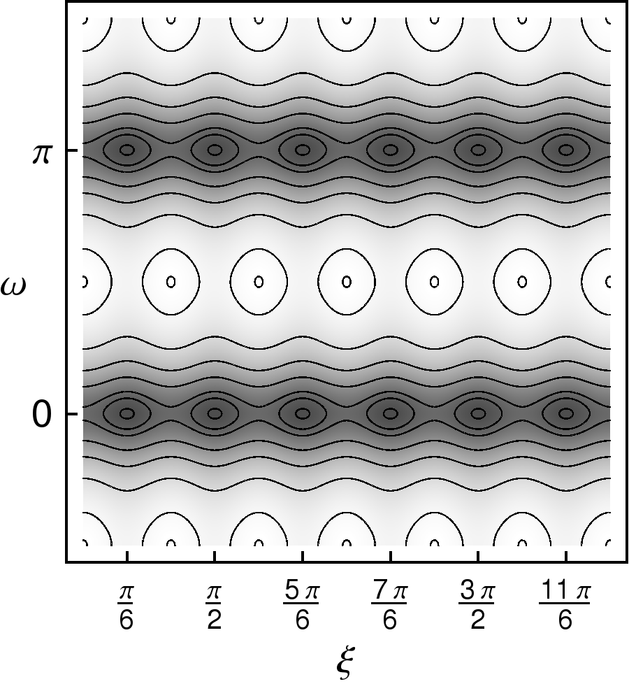
Figure 1: Effective potential (2) as a function of the angle $\omega$ between chromomagnetic and chromoelectric field and the mixing angle $\xi$ in the Cartan subalgebra. The minima in the dark gray regions correspond to the Abelian (anti-)self-dual configurations and form a periodic structure labelled by integer indices $(kl)$ in Eq. (3) (for more details see NK1 ; NG2011 ; NV ).

Ginzburg-Landau (GL) approach to the quantum effective action indicated a possibility of the domain wall network formation in QCD vacuum resulting in the dominating vacuum gluon configuration seen as an ensemble of densely packed lumps of covariantly constant Abelian (anti-)self-dual field NK1 ; NG2011 ; NV ; George:2012sb . Nonzero scalar gluon condensate $\langle g^{2}F^{a}_{\mu\nu}F^{a}_{\mu\nu}\rangle$ postulated by the effective potential

$$U_{\mathrm{eff}} = \frac{\Lambda^{4}}{12}{\rm Tr}\left(C_{1}\breve{f}^{2}+\frac{4}{3}C_{2}\breve{f}^{4}-\frac{16}{9}C_{3}\breve{f}^{6}\right),$$ (2)

with $\Lambda$ being a scale of QCD and $\breve{f}_{\mu\nu}=\breve{T}^{a}F^{a}_{\mu\nu}/\Lambda^{2}$, leads to the existence of twelve discrete degenerate global minima of the effective action (see Fig.1),

$$\breve{A}_{\mu}\in\left\{\breve{B}^{(kl)}_{\mu}|\ k=0,1,\dots,5;\ l=0,1\right\},\ \ \breve{B}^{(kl)}_{\mu}=-\frac{1}{2}\breve{n}_{k}B^{(l)}_{\mu\nu}x_{\nu},$$

$$\tilde{B}^{(l)}_{\mu\nu}=\frac{1}{2}\varepsilon_{\mu\nu\alpha\beta}B^{(l)}_{\alpha\beta}=(-1)^{l}B^{(l)}_{\mu\nu},$$

$$\breve{n}_{k}=T^{3}\ \cos\left(\xi_{k}\right)+T^{8}\ \sin\left(\xi_{k}\right),\ \ \xi_{k}=\frac{2k+1}{6}\pi,$$ (3)

where $l=0$ and $l=1$ correspond to the self-dual and anti-self-dual field respectively, matrix $\breve{n}_{k}$ belongs to Cartan subalgebra of $su(3)$ with six values of the angle $\xi_{k}$ corresponding to the boundaries of the Weyl chambers in the root space of $su(3)$.

The minima are connected by the parity and Weyl group reflections. Their existence indicates that the system is prone to the domain wall formation. To demonstrate the simplest example of domain wall interpolating between the self-dual and anti-self-dual Abelian configurations, one allows the angle $\omega$ between chromomagnetic and chromoelectric fields to vary from point to point in $R^{4}$ and restricts other degrees of freedom of gluon field to their vacuum values. In this case Ginsburg-Landau Lagrangian leads to the sine-Gordon equation for $\omega$ with the standard kink solution (for details see Ref. NG2011 ; NV )

$$\omega(x_{\nu})=2\ \arctan\left(\exp(\mu x_{\nu})\right).$$

Away from the kink location vacuum field is almost self-dual ($\omega=0$) or anti-self-dual ($\omega=\pi$). Exactly at the wall it becomes purely chromomagnetic ($\omega=\pi/2$). Domain wall network is constructed by means of the kink superposition. In general kink can be parametrized as

$$\zeta(\mu_{i},\eta_{\nu}^{i}x_{\nu}-q^{i})=\frac{2}{\pi}\arctan\exp(\mu_{i}(\eta_{\nu}^{i}x_{\nu}-q^{i})),$$

where $\mu^{i}$ is inverse width of the kink, $\eta_{\nu}^{i}$ is a normal to the wall and $q^{i}=\eta_{\nu}^{i}x_{\nu}$ are coordinates of the wall. A single lump in two, three and four dimensions is given by

$$\omega(x)=\pi\prod_{i=1}^{k}\zeta(\mu_{i},\eta_{\nu}^{i}x_{\nu}-q^{i}).$$

for $k=4,6,8$, respectively. The general kink network is then given by the additive superposition of lumps

$$\omega=\pi\sum_{j=1}^{\infty}\prod_{i=1}^{k}\zeta(\mu_{ij},\eta_{\nu}^{ij}x_{\nu}-q^{ij}).$$

Topological charge density distribution for a network of domain walls with different width is illustrated in Fig.2.

Based on this construction, the measure of integration over the background field $B_{\mu}^{a}$ can be constructively represented as the infinite dimensional (in the infinite volume) integral over the parameters of $N\to\infty$ domain walls in the network: their positions, orientations and widths, with the weight determined by the effective action. It should be noted that chronologically the explicit construction of the domain wall network is the most recent development of the formalism that have been studied in the series of papers EN ; EN1 ; NK1 ; NK4 ; NK6 , in which the domain wall defects in the homogeneous Abelian (anti-)self-dual field were taken into account either implicitly or in an explicit but simplified form with the spherical domains. The practical calculations in the next sections will be done within combined implementation of domain model given in paper NK4 : propagators in the quark loops are taken in the approximation of the homogeneous background field and the quark loops are averaged over the background field, the correlators of the background field are calculated in the spherical domain approximation.

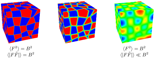
Figure 2: Topological charge density for domain wall networks with different values of the wall width $\mu$. The leftmost picture is an example of confining almost everywhere homogeneous Abelian (anti-)self-dual fields. Red (blue) color corresponds to the self-dual field (anti-self-dual), green – pure chromomagnetic field. The rightmost plot represents the case of preferably pure chromomagnetic field when the topological charge density is nearly zero and color charged quasiparticles can be excited thus indicating deconfinement (for more details see NV ).

III Hadronization within the domain model of QCD vacuum

The haronization formalism based on domain model of QCD vacuum was elaborated in the series of papers EN1 ; EN ; NK1 ; NK4 . We refer to these papers for most of the technical details omitted in this brief presentation. It has been shown that the model embraces static (area law) and dynamical quark confinement (propagators in momentum representation are entire analytical functions) as well as spontaneous breaking of chiral symmetry by the background domain structured field itself. $U_{A}(1)$ problem was resolved without introducing the strong CP-violation NK6 . Estimation of masses of light, heavy-light mesons and heavy quarkonia along with their orbital excitations EN1 ; EN ; NK4 demonstrated promising phenomenological performance. However, calculations in Refs. EN ; NK4 have been done neglecting a mixing between radially excited meson fields. Below we present results of calculation refined in this respect.

In the spherical domain approximation, the background gluon fields are represented by the ensemble of domain-structured fields with the strength tensor NK1 ; NK4

$$F^{a}_{\mu\nu}(x)=\sum_{k=1}^{N}n^{(k)a}B^{(k)}_{\mu\nu}\theta(1-(x-z_{k})^{2}/R^{2}),\quad B^{(k)}_{\mu\nu}B^{(k)}_{\mu\rho}=B^{2}\delta_{\nu\rho},\quad B=\frac{2}{\sqrt{3}}\Lambda^{2},$$

$$\tilde{B}^{(k)}_{\mu\nu}=\pm B^{(k)}_{\mu\nu},\quad\hat{n}^{(k)}=t^{3}\cos\xi_{k}+t^{8}\sin\xi_{k},\quad\xi_{k}\in\left\{\frac{\pi}{6}(2k+1),\ k=0,\dots,5\right\},$$

where $z_{k}$ is the space-time coordinate of the $k$-th domain center, scale $\Lambda$ and mean domain radius $R$ are parameters of the model related to the scalar gluon condensate and topological susceptibility of pure Yang-Mills vacuum, respectively NK1 .

The measure of integration over ensemble of background fields is defined as NK1 ; NK4

$$\int\limits_{\cal B}dB\dots = \prod_{k}\frac{1}{24\pi^{2}}\lim_{V\to\infty}\frac{1}{V}\int_{V}d^{4}z_{k}\int\limits_{0}^{2\pi}d\varphi_{k}\int_{0}^{\pi}d\theta_{k}\sin\theta_{k}$$

$$\times \int_{0}^{2\pi}d\xi_{k}\sum\limits_{l=0,1,2}^{3,4,5}\delta\left(\xi_{k}-\frac{(2l+1)\pi}{6}\right)\int_{0}^{\pi}d\omega_{k}\sum\limits_{n=0,1}\delta(\omega_{k}-\pi n)\dots$$

Once the measure is specified, one can return to the functional integral (1) and integrate out fluctuation part of the gluon fields $Q$:

$${\cal Z} = \int dB\int_{\Psi}{\cal D}\psi{\cal D}\bar{\psi}\int_{{\cal Q}}{\cal D}Q\delta[D(B)Q]\Delta_{\rm FP}[B,Q]e^{-S^{\rm QCD}\left[Q+B,\psi,\bar{\psi}\right]}$$

$$= \int dB\int_{\Psi}{\cal D}\psi{\cal D}\bar{\psi}\exp\left\{\int dx\bar{\psi}\left(i\not{\partial}+g\not{B}-m\right)\psi\right\}W[j],$$

where $j^{a}_{\mu}(x)=\bar{\psi}(x)\gamma_{\mu}t^{a}\psi(x)$ is the local quark current. Recalling the definition of Green functions,

$$G^{a_{1}\dots a_{n}}_{\mu_{1}\dots\mu_{n}}(x_{1},\dots,x_{n}|B)=\left.\frac{1}{g^{n}}\frac{\delta^{n}\ln W[j]}{\delta j^{a_{1}}_{\mu_{1}}(x_{1})\dots\delta j^{a_{n}}_{\mu_{n}}(x_{n})}\right\lvert_{j=0},$$

we arrive at the representation

$$W[j|B] = \exp\left\{\sum_{n}\frac{g^{n}}{n!}\int d^{4}x_{1}\dots\int d^{4}x_{n}j^{a_{1}}_{\mu_{1}}(x_{1})\dots j^{a_{n}}_{\mu_{n}}(x_{n})G^{a_{1}\dots a_{n}}_{\mu_{1}\dots\mu_{n}}(x_{1},\dots,x_{n}|B)\right\},$$

where by construction the gauge coupling constant $g$ and the exact renormalized $n$-point gluon Green functions of pure gauge theory in the presence of the background field $B$ appear to be renormalized within appropriate renormalization scheme. It is needless to say that the functional form of these Green functions, gluon propagator in particular, has been a subject of many investigations carried out over decades. Quite reliable information about two- and three-point Euclidean Green functions was obtained within the functional renormalization group, Lattice QCD as well as calculations based on Dyson-Schwinger equations.

At this step one has to set up the approximation scheme. We truncate the exponent in $W[j|B]$ up to the four-fermion interaction term. Interaction between standard local color charged quark currents is described by the product of the renormalized coupling constant squared and exact gluon propagator $g^{2}G^{a_{1}a_{2}}_{\mu_{1}\mu_{2}}(x_{1},x_{2}|B)$ which will be approximated by the gluon propagator in the presence of homogeneous Abelian (anti-)self-dual field. Radiative corrections due to the gluon and ghost field fluctuations are neglected (for more details see Refs. EN1 ; EN ; NK4 ). It should be noted that omitted radiative corrections can be represented in terms of the standard for pure gluodynamics set of Feynman graphs for gluon polarization function but the internal lines in the graphs correspond to the gluon and ghost propagators in the background field $B$. In other words, the approximation in use corresponds to the lowest (tree level) order with respect to perturbative fluctuations $Q$, but the background field (vacuum field $B$) itself is taken into account exactly.

The randomness of domain ensemble is taken into account implicitly by means of averaging the nonlocal meson-meson interaction vertices over all possible configurations of the homogeneous background field at the final stage of derivation of the effective meson action EN ; NK4 .

Relevant truncated part of QCD functional integral reads

$$\mathcal{Z}=\int_{\cal B}dB\int_{\Psi}{\cal D}\psi{\cal D}\bar{\psi}\exp\left\{\int d^{4}x\bar{\psi}\left(i\not{\partial}+g\not{B}-m\right)\psi+\mathcal{L}\right\},$$ (4)

$$\mathcal{L}=\frac{g^{2}}{2}\int d^{4}x\int d^{4}y\ G^{ab}_{\mu\nu}(x,y|B)j^{a}_{\mu}(x)j^{b}_{\nu}(y),$$

where $m$ is a diagonal quark mass matrix. By means of the standard Fierz transformation of color, Dirac and flavour matrices the four-quark interaction can be rewritten as

$$\mathcal{L}=\frac{g^{2}}{2}\sum_{J,c}C_{J}\int d^{4}x\int d^{4}yG(x-y)J^{Jc}(x,y|B)J^{Jc}(y,x|B),$$

where numerical coefficients $C_{J}$ are different for different spin-parity $J=S,P,V,A$. Here bilocal color neutral quark currents,

$$J^{Jc}(x,y|B)=\bar{\psi}(x)\lambda^{c}\Gamma_{J}\exp\left\{\frac{i}{2}x_{\mu}\hat{B}_{\mu\nu}y_{\nu}\right\}\psi(y),$$

are singlets with respect to the local background gauge transformations. In the center of quark mass coordinate system bilocal currents take the form

$$J^{Jc}(x,y|B)\to J^{Jc}(x,z|B)=\bar{\psi}_{f}(x)\lambda^{c}\Gamma_{J}\exp\left(iz_{\mu}\stackrel{{\scriptstyle\leftrightarrow}}{{\mathcal{D}_{ff^{\prime}}^{\mu}}}(x)\right)\psi_{f^{\prime}}(x),$$ (5)

$$\stackrel{{\scriptstyle\leftrightarrow}}{{\mathcal{D}^{ff^{\prime}}_{\mu}}}=\xi_{f}\stackrel{{\scriptstyle\leftarrow}}{{\mathcal{D}}}_{\mu}-\xi_{f^{\prime}}\stackrel{{\scriptstyle\rightarrow}}{{\mathcal{D}}}_{\mu},\ \ \stackrel{{\scriptstyle\leftarrow}}{{\mathcal{D}}}_{\mu}(x)=\stackrel{{\scriptstyle\leftarrow}}{{\partial}}_{\mu}+i\hat{B}_{\mu}(x),\ \ \stackrel{{\scriptstyle\rightarrow}}{{\mathcal{D}}}_{\mu}(x)=\stackrel{{\scriptstyle\rightarrow}}{{\partial}}_{\mu}-i\hat{B}_{\mu}(x),$$

$$\xi_{f}=\frac{m_{f^{\prime}}}{m_{f}+m_{f^{\prime}}},\ \xi_{f^{\prime}}=\frac{m_{f}}{m_{f}+m_{f^{\prime}}},$$

and their interaction is described by the action EN1

$$\mathcal{S}=\frac{g^{2}}{2}\sum_{J,c}C_{J}\int d^{4}x\int d^{4}zG(z)J_{Jc}^{\dagger}(x,z|B)J_{Jc}(x,z|B),$$ (6)

$$G(z)=\frac{1}{4\pi^{2}z^{2}}\exp\left\{-\frac{1}{4}\Lambda^{2}z^{2}\right\},$$ (7)

where $x_{\mu}$ - center of quark mass coordinates, and $z_{\mu}$ - relative coordinates of quark and antiquark. It has to be noted here that quark fields are seen as pure fluctuations describable in terms of four-dimentional harmonic oscillator eigenmodes of the bound state type NV ; NK1 ; NK4 in $R^{4}$. Interpretation of the quark field in terms of point-like particle is simply does not exist in the confining background under consideration. Function $G(z)$ originates from the gluon propagator in the presence of the homogeneous Abelian (anti-)self-dual gluon field EN1 . It differs from the free massless scalar propagator by the Gaussian exponent, which completely changes the IR properties of the propagator but leaves its UV asymptotic behaviour unchanged. In momentum representation it takes the form

$$\tilde{G}\left(p\right)=\frac{1}{p^{2}}\left(1-e^{-p^{2}/\Lambda^{2}}\right).$$ (8)

It is important that nonzero gluon condensates $\langle g^{2}F^{2}\rangle$ and $\langle g^{2}|\tilde{F}F|\rangle$ represented by the Abelian (anti-)self-dual vacuum field remove the pole from the propagator which can be treated as dynamical confinement of the color charged fields Leutwyler1 .

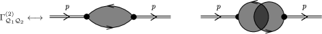
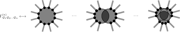
Figure 3: Diagrammatic representation of nonlocal meson vertex functions. Light grey denotes averaging over background field, dark grey denotes correlation of loop diagrams by background field.

The quark propagator in the homogeneous as well as domain structured NK1 Abelian (anti-)self-dual gluon field also demonstrates confinement. Momentum representation $\tilde{H}_{f}(p|B)$ of the translation invariant part of the quark propagator in the presence of the homogeneous field,

$$S(x,y)=\exp\left(-\frac{i}{2}x_{\mu}B_{\mu\nu}y_{\nu}\right)H(x-y),$$

is an entire analytical function of momentum:

$$\tilde{H}_{f}(p)=\frac{1}{2v\Lambda^{2}}\int_{0}^{1}dse^{(-p^{2}/2v\Lambda^{2})s}\left(\frac{1-s}{1+s}\right)^{m_{f}^{2}/4v\Lambda^{2}}\left[\vphantom{\frac{s}{1-s^{2}}}p_{\alpha}\gamma_{\alpha}\pm is\gamma_{5}\gamma_{\alpha}f_{\alpha\beta}p_{\beta}\right.$$

$$\left.\mbox{}+m_{f}\left(P_{\pm}+P_{\mp}\frac{1+s^{2}}{1-s^{2}}-\frac{i}{2}\gamma_{\alpha}f_{\alpha\beta}\gamma_{\beta}\frac{s}{1-s^{2}}\right)\right],$$ (9)

$$f_{\alpha\beta}=\frac{\hat{n}}{2v\Lambda^{2}}B_{\alpha\beta},\ v=\mathrm{diag}\left(\frac{1}{6},\frac{1}{6},\frac{1}{3}\right),\ \ \hat{B}_{\rho\mu}\hat{B}_{\rho\nu}=4v^{2}\Lambda^{4}\delta_{\mu\nu}.$$

The propagator has a rich Dirac structure including not only the vector and scalar parts but also the pseudoscalar, axial vector and tensor terms (flavour index $f$ is omitted for the sake of brevity)

$$\tilde{H}(p)=\frac{m}{2v\Lambda^{2}}{\cal H}_{S}(p^{2})\mp\gamma_{5}\frac{m}{2v\Lambda^{2}}{\cal H}_{P}(p^{2})+\gamma_{\alpha}\frac{p_{\alpha}}{2v\Lambda^{2}}{\cal H}_{V}(p^{2})\pm i\gamma_{5}\gamma_{\alpha}\frac{f_{\alpha\beta}p_{\beta}}{2v\Lambda^{2}}{\cal H}_{A}(p^{2})+\sigma_{\alpha\beta}\frac{mf_{\alpha\beta}}{4v\Lambda^{2}}{\cal H}_{T}(p^{2}).$$ (10)

Here ”$\pm$” corresponds to self-dual and anti-self-dual background field configurations. One can easily reconstruct explicit form of functions $\mathcal{H}_{J}$ from Eq.(III). More detailed description of different form factors, particularly the scalar one, and their role in the chiral symmetry realization will be given in section V. This structure of the quark propagator plays important role for successful description of the meson spectrum, especially for the ground state light mesons.

Table 1: Model parameters fitted to the masses of $\pi,\rho,K,K^{*},\eta^{\prime},J/\psi,\Upsilon$ and used in calculation of all other meson masses, decay and transition constants, for $N=7$ (see explanations in the text and Fig.4).

$m_{u/d}$, MeV	$m_{s}$, MeV	$m_{c}$, MeV	$m_{b}$, MeV	$\Lambda$, MeV	$\alpha_{s}$	$R$, fm
$145$	$376$	$1566$	$4879$	$416$	$3.45$	$1.12$

There are two equivalent ways to derive effective meson action based on the functional integral (4) with the interaction term $\mathcal{L}$ taken in the form (6). The first one is bosonization of the functional integral in terms of bilocal meson-like fields (see for example Ref. roberts ). We shall return to this option in the discussion section. Another, more elucidative way is to decompose the bilocal currents (5) over complete set of functions $f^{nl}_{\mu_{1}\dots\mu_{l}}(z)$ orthogonal with the weight determined by function $G(z)$ originating from the gluon propagator (7) in Eq.(6)

$$J^{aJ}(x,z)=\sum_{n,l=0}^{\infty}\left(z^{2}\right)^{l/2}f^{nl}_{\mu_{1}\dots\mu_{l}}(z)J^{aJln}_{\mu_{1}\dots\mu_{l}}(x).$$

Here $n$ is the radial quantum number and $l$ is the orbital momentum. Coefficient quark currents $J^{aJln}_{\mu_{1}\dots\mu_{l}}(x)$ have to describe intrinsic structure of the collective meson-like excitations with complete set of quantum numbers. The form of interaction (6) and natural requirement of diagonality (with respect to $n$ and $l$) of the four-quark interaction, expressed in terms of the currents $J^{aJln}_{\mu_{1}\dots\mu_{l}}(x)$, indicate the choice of $f^{nl}(z)$

$$f^{nl}_{\mu_{1}\dots\mu_{l}}=L_{nl}\left(z^{2}\right)T^{(l)}_{\mu_{1}\dots\mu_{l}}(n_{z}),\quad n_{z}=z/\sqrt{z^{2}}.$$ (11)

Here $T^{(l)}_{\mu_{1}\dots\mu_{l}}$ are irreducible tensors of four-dimensional rotational group, and generalized Laguerre polynomials $L_{nl}$ obey relation

$$\int_{0}^{\infty}du\rho_{l}(u)L_{nl}(u)L_{n^{\prime}l}(u)=\delta_{nn^{\prime}},\quad\rho_{l}(u)=u^{l}e^{-u}.$$

The weight $\rho_{l}(u)$ comes from the gluon propagator (7). Nonlocal quark currents $J^{aJln}_{\mu_{1}\dots\mu_{l}}$ with complete set of meson quantum numbers can be explicitly calculated and depend only on the center of mass coordinate $x$ EN ; NK4 ,

$$J^{aJln}_{\mu_{1}\dots\mu_{l}}(x)=\bar{q}(x)V^{aJln}_{\mu_{1}\dots\mu_{l}}\left(\frac{\stackrel{{\scriptstyle\leftrightarrow}}{{D}}\!(x)}{\Lambda}\right)q(x),$$

$$V^{aJln}_{\mu_{1}\dots\mu_{l}}(x)={\cal C}_{Jln}M^{a}\Gamma^{J}F_{nl}\left(\frac{\stackrel{{\scriptstyle\leftrightarrow}}{{\cal D}}^{2}\!\!\!(x)}{\Lambda^{2}}\right)T^{(l)}_{\mu_{1}\dots\mu_{l}}\left(\frac{1}{i}\frac{\stackrel{{\scriptstyle\leftrightarrow}}{{\cal D}}\!(x)}{\Lambda}\right),$$ (12)

$$F_{nl}(s)=s^{n}\int_{0}^{1}dtt^{n+l}\exp(st),$$

$${\cal C}^{2}_{Jln}=C_{J}\frac{l+1}{2^{l}n!(n+l)!},\quad C_{S/P}=2C_{V/A}=\frac{1}{9},$$

where $M^{a}$ and $\Gamma^{J}$ are flavour $SU(N_{f})$ and Dirac matrices respectively. The four-fermion interaction takes the form of an infinite sum of the current-current interactions diagonal with respect to all quantum numbers

$$\mathcal{L}=\frac{g^{2}}{2}\sum_{aJln}\int d^{4}xJ_{aJln}^{\dagger}(x)J_{aJln}(x).$$

It has to be stressed that the nonlocal quark currents are invariant with respect to the local gauge transformations of the background gauge field as the vertices (12) depend on the covariant derivatives.

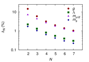
Figure 4: Dependence of relative variation of the model parameters $\Delta_{N}=|P_{N}-P_{N-1}|/P_{N-1}$ on the number of Laguerre polynomials $N$ taken into account during diagonalization of the quadratic part of the meson action with respect to the radial number $n$. It can be seen that the iterations converge with $N$ for all quantities faster than $\Delta_{N}\approx\Delta_{1}\exp(-.35N)$ for $N>5$. For $N=7$ the variations of light quark mass $m_{u/d}$ and coupling constant $g$ slow down to one percent level, while the change of the scale $\Lambda$ and the strange quark mass $m_{s}$ approach a fraction of a percent. Alternations of the masses of heavy $c$ and $b$ quarks and domain size $R$ are not shown as it is of order of $.1\%$ or less for any $N$ which is far smaller than the overall accuracy of the model.

The truncated QCD functional integral can be rewritten in terms of the composite colorless meson fields $\phi_{\cal Q}$ by means of the standard bosonization procedure: introduce the auxiliary meson fields, integrate out the quark fields, perform the orthogonal transformation of the auxiliary fields that diagonalizes the quadratic part of the action and, finally, rescale the meson fields to provide the correct residue of the meson propagator at the pole corresponding to its physical mass (if any). More details can be found in Ref. EN ; EN1 ; NK4 . The result can be written in the following compact form

$$Z={\cal N}\int D\phi_{\cal Q}\exp\left\{-\frac{\Lambda^{2}}{2}\frac{h^{2}_{\cal Q}}{g^{2}}\int d^{4}x\phi^{2}_{\cal Q}(x)-\sum\limits_{k=2}^{\infty}\frac{1}{k}W_{k}[\phi]\right\},$$ (13)

$$W_{k}[\phi]=\sum\limits_{{\cal Q}_{1}\dots\cal Q_{k}}h_{{\cal Q}_{1}}\dots h_{{\cal Q}_{k}}\int d^{4}x_{1}\dots\int d^{4}x_{k}\Phi_{{\cal Q}_{1}}(x_{1})\dots\Phi_{{\cal Q}_{k}}(x_{k})\Gamma^{(k)}_{{\cal Q}_{1}\dots\cal Q_{k}}(x_{1},\dots,x_{k}),$$ (14)

$$\Phi_{{\cal Q}}(x)=\int\frac{d^{4}p}{(2\pi)^{4}}e^{ipx}{\mathcal{O}}_{{\mathcal{Q}}{\mathcal{Q}}^{\prime}}(p)\tilde{\phi}_{{\mathcal{Q}}^{\prime}}(p),$$ (15)

where condensed index $\mathcal{Q}$ denotes all relevant meson quantum numbers and indices. Integration variables $\phi_{\mathcal{Q}}$ in the functional integral (13) correspond to the physical meson fields that diagonalize the quadratic part of the effective meson action (14) in momentum representation, which is achieved by means of orthogonal transformation ${\mathcal{O}}(p)$.

Interactions between physical meson fields $\phi_{\mathcal{Q}}$ are described by $k$-point nonlocal vertices $\Gamma^{(k)}_{\mathcal{Q}_{1}\dots\mathcal{Q}_{2}}$,

$$\Gamma^{(2)}_{{\cal Q}_{1}{\cal Q}_{2}}=\overline{G^{(2)}_{{\cal Q}_{1}{\cal Q}_{2}}(x_{1},x_{2})}-\Xi_{2}(x_{1}-x_{2})\overline{G^{(1)}_{{\cal Q}_{1}}G^{(1)}_{{\cal Q}_{2}}},$$

$$\Gamma^{(3)}_{{\cal Q}_{1}{\cal Q}_{2}{\cal Q}_{3}}=\overline{G^{(3)}_{{\cal Q}_{1}{\cal Q}_{2}{\cal Q}_{3}}(x_{1},x_{2},x_{3})}-\frac{3}{2}\Xi_{2}(x_{1}-x_{3})\overline{G^{(2)}_{{\cal Q}_{1}{\cal Q}_{2}}(x_{1},x_{2})G^{(1)}_{{\cal Q}_{3}}(x_{3})}$$

$$+\frac{1}{2}\Xi_{3}(x_{1},x_{2},x_{3})\overline{G^{(1)}_{{\cal Q}_{1}}(x_{1})G^{(1)}_{{\cal Q}_{2}}(x_{2})G^{(1)}_{{\cal Q}_{3}}(x_{3})},$$

$$\Gamma^{(4)}_{{\cal Q}_{1}{\cal Q}_{2}{\cal Q}_{3}{\cal Q}_{4}}=\overline{G^{(4)}_{{\cal Q}_{1}{\cal Q}_{2}{\cal Q}_{3}{\cal Q}_{4}}(x_{1},x_{2},x_{3},x_{4})}-\frac{4}{3}\Xi_{2}(x_{1}-x_{2})\overline{G^{(1)}_{{\cal Q}_{1}}(x_{1})G^{(3)}_{{\cal Q}_{2}{\cal Q}_{3}{\cal Q}_{4}}(x_{2},x_{3},x_{4})}$$

$$-\frac{1}{2}\Xi_{2}(x_{1}-x_{3})\overline{G^{(2)}_{{\cal Q}_{1}{\cal Q}_{2}}(x_{1},x_{2})G^{(2)}_{{\cal Q}_{3}{\cal Q}_{4}}(x_{3},x_{4})}$$

$$+\Xi_{3}(x_{1},x_{2},x_{3})\overline{G^{(1)}_{{\cal Q}_{1}}(x_{1})G^{(1)}_{{\cal Q}_{2}}(x_{2})G^{(2)}_{{\cal Q}_{3}{\cal Q}_{4}}(x_{3},x_{4})}$$

$$-\frac{1}{6}\Xi_{4}(x_{1},x_{2},x_{3},x_{4})\overline{G^{(1)}_{{\cal Q}_{1}}(x_{1})G^{(1)}_{{\cal Q}_{2}}(x_{2})G^{(1)}_{{\cal Q}_{3}}(x_{3})G^{(1)}_{{\cal Q}_{4}}(x_{4})},$$

subsequently tuned to the physical meson representation by means of corresponding orthogonal transformations ${\mathcal{O}}(p)$. Vertices $\Gamma^{(k)}$ are expressed via 1-loop diagrams $G^{(k)}_{{\cal Q}_{1}\dots\cal Q_{k}}$ which include nonlocal quark-meson vertices (12) and quark propagators (III) :

$$\overline{G^{(k)}_{{\cal Q}_{1}\dots\cal Q_{k}}(x_{1},\dots,x_{k})}=\int dB{\rm Tr}V_{{\cal Q}_{1}}\left(x_{1}|B\right)S\left(x_{1},x_{2}\right)\dots V_{{\cal Q}_{k}}\left(x_{k}|B\right)S\left(x_{k},x_{1}\right),$$

$$\overline{G^{(l)}_{{\cal Q}_{1}\dots\cal Q_{l}}(x_{1},\dots,x_{l})G^{(k)}_{{\cal Q}_{l+1}\dots\cal Q_{k}}(x_{l+1},\dots,x_{k})}=\\ \int dB{\rm Tr}\left\{V_{{\cal Q}_{1}}\left(x_{1}|B\right)S\left(x_{1},x_{2}|B\right)\dots V_{{\cal Q}_{k}}\left(x_{l}|B\right)S\left(x_{l},x_{1}|B\right)\right\}\\ \times{\rm Tr}\left\{V_{{\cal Q}_{l+1}}\left(x_{l+1}|B\right)S\left(x_{l+1},x_{l+2}|B\right)\dots V_{{\cal Q}_{k}}\left(x_{k}|B\right)S\left(x_{k},x_{l+1}|B\right)\right\}.$$

Bar denotes integration over all configurations of the background fields. As it is illustrated in Fig.3, vertex functions $\Gamma^{(k)}$ include, in general, several one-loop diagrams correlated via the background field. In the simplified model of spherical domains, the $n$-point correlator $\Xi_{n}(x_{1},\dots,x_{n})$ is given by a volume of overlap of $n$ four-dimensional hyperspheres NK1 ; NK4 .

It has to be noted that though all Dirac structures, besides the vector and scalar ones, are nullified by the integration of the propagator (10) over the background field, all of them give highly nontrivial contribution to the quark loops (products of several propagators). For example, the two-point correlators responsible for the mass spectrum contain not only the one gluon (fluctuation $Q$!) exchange interaction hidden in the vertex $V_{\cal Q}$ but also additional $S$, $P$, $V$, $A$ and $T$ interactions effectively generated by the background gluon field $B$.

It has to be stressed that the terms linear in meson fields are absent in (13). The linear terms naturally vanish for all mesons besides the scalar ones, and their elimination for the scalar fields requires solution of an infinite system of equations

$$\Lambda^{2}\Phi_{{\cal Q}_{1}}^{(0)}=\sum\limits_{k=1}^{\infty}\frac{g^{k}}{k}\sum\limits_{{\cal Q}_{1}\dots\cal Q_{k}}\Phi^{(0)}_{{\cal Q}_{2}}\dots\Phi^{(0)}_{{\cal Q}_{k}}\Gamma^{(k)}_{{\cal Q}_{1}\dots\cal Q_{k}},$$ (16)

where ${\cal Q}_{k}=\{a_{k}S0n_{k}\}$ and $\Phi^{(0)}_{{\cal Q}_{k}}=\mathrm{const}$ can be treated as an infinite set of scalar quark condensates labelled by the radial quantum number $n$. As we shall discuss in section V, solution of this system of equations leads to the interesting details of the chiral symmetry realization in the presence of the background field under consideration. Actual calculations further below will be done with constant mass which from now on will be treated as the infrared limit of the running nonperturbative quark masses $m_{f}(0)$ considered as parameters of the model.

Table 2: Masses of light mesons. $\tilde{M}$ denotes the value in the chiral limit.

Meson	$n$	$M_{\rm exp}$PDG	$M$	$\tilde{M}$	$h$	Meson	$n$	$M_{\rm exp}$PDG	$M$	$\tilde{M}$	$h$
		( MeV)	(MeV)	(MeV)				( MeV)	(MeV)	(MeV)
$\pi$	0	140	140	0	3.63	$\rho$	0	775	775	769	1.83
$\pi(1300)$	1	1300	1310	1301	2.74	$\rho(1450)$	1	1450	1571	1576	1.44
$\pi(1800)$	1	1812	1503	1466	2.83	$\rho$	2	1720	1946	2098	1.58
$K$	0	494	494	0	4.13	$K^{*}$	0	892	892	769	1.99
$K(1460)$	1	1460	1302	1301	1.97	$K^{*}(1410)$	1	1410	1443	1576	1.38
$K$	2		1655	1466	1.96	$K^{*}$	2		1781	2098	1.44
$\eta$	0	548	610	0	3.74	$\omega$	0	775	775	769	1.83
$\eta^{\prime}$	0	958	958	872	2.73	$\phi$	0	1019	1039	769	2.21
$\eta(1295)$	1	1294	1138	1361	2.62	$\phi(1680)$	1	1680	1686	1576	1.55
$\eta(1475)$	1	1476	1297	1516	2.41	$\phi$	2	2175	1897	2098	1.55

The mass spectrum $M_{\mathcal{Q}}$ of mesons and quark-meson coupling constants $h_{\cal Q}$ are determined by the quadratic part of the effective meson action via equations

$$1=\frac{g^{2}}{\Lambda^{2}}\tilde{\Pi}_{\cal Q}(-M^{2}_{\cal Q}|B),$$ (17)

$$h^{-2}_{\cal Q}=\frac{d}{dp^{2}}\tilde{\Pi}_{\cal Q}(p^{2})|_{p^{2}=-M^{2}_{\cal Q}},$$ (18)

where $\tilde{\Pi}_{\cal Q}(p^{2})$ is the diagonalized two-point correlator $\tilde{\Gamma}^{(2)}_{\cal QQ^{\prime}}(p)$ put on mass shell:

$$\tilde{\phi}^{\dagger}_{\mathcal{Q}}(-p)\left[\mathcal{O}^{T}(p)\tilde{\Gamma}^{(2)}(p)\mathcal{O}(p)\right]_{\cal QQ^{\prime}}\tilde{\phi}_{{\mathcal{Q}}^{\prime}}(p)|_{p^{2}=-M^{2}_{\cal Q}}=\tilde{\Pi}_{\cal Q}(-M_{\mathcal{Q}}^{2})\tilde{\phi}^{\dagger}_{\mathcal{Q}}(-p)\tilde{\phi}_{\mathcal{Q}}(p)|_{p^{2}=-M^{2}_{\cal Q}}.$$

Explicit construction of $\tilde{\Pi}_{\cal Q}(p^{2})$ will be discussed in the next section. Solution of Eq. (17) identifies the position of the pole in the propagator of the meson with quantum numbers ${\cal Q}$. Definition (18) of the meson-quark coupling constant $h_{\cal Q}$ provides correct residue at the pole.

The free parameters of the model are the IR limits of the running renormalized strong coupling constant $\alpha_{s}$, quark masses $m_{u}=m_{d}$, $m_{s}$, $m_{c}$, $m_{b}$, and the scales $\Lambda$ and $R$. By construction, the coupling constant and the quark masses correspond to the background Feynman gauge condition and momentum subtraction (MOM) renormalization scheme at subtraction point $p^{2}=0$ . The scale $\Lambda$ and mean domain size $R$ are related to the scalar gluon condensate and topological susceptibility of pure gluodynamics respectively,

$$\langle\alpha_{s}F^{2}\rangle=\frac{2}{3}\frac{\Lambda^{4}}{\pi},\quad\chi_{\mathrm{YM}}=\frac{1}{72}\frac{\Lambda^{8}R^{4}}{128\pi^{2}}.$$

It should be noted that decomposition (11) and (12) attributes the same radial form factor $F_{nl}$ to the mesons with different spin-parity $J$. Moreover, the form of $F_{nl}$ appears to be the same for all quarkonium-like collective excitations with different quark content and spin-parity such as $\pi$ and $J/\psi$ mesons. On the contrary, the physical meson states correspond to the momentum dependent transformed basis and respectively transformed quark current

$$f_{p}^{aJln}(z)=\sum_{n^{\prime}=0}^{\infty}{\mathcal{O}}_{aJl}^{nn^{\prime}}(p)f^{ln^{\prime}}(z),\ \ {\mathcal{O}}_{aJl}{\mathcal{O}}_{aJl}^{T}=I,$$

$$\tilde{J}^{aJ}(p,z)=\sum_{nl}^{\infty}\left(z^{2}\right)^{l/2}f^{aJnl}_{p}(z)\mathcal{O}^{nn^{\prime}}_{aJl}\tilde{J}^{aJln^{\prime}}(p),$$

where ${{\mathcal{O}}_{aJl}(p)}$ is an orthogonal transformation of the initial basis taking into account two-point function $\tilde{\Gamma}_{\mathcal{QQ}^{\prime}}^{(2)}(p)$. All this means that though ab initio the basic property of quark-meson interaction form factor is set up by gluon propagator, it is the quark loop that defines its final physical form which is different for different mesons.

IV Masses and decay constants of mesons

IV.1 Mass spectrum of radial excitations of light, heavy-light mesons and heavy quarkonia

Meson masses are defined by the algebraic equation (17). This equation emerges as follows. In the momentum representation, the quadratic part of the effective action pseudoscalar and vector meson fields with zero orbital momentum has the form

$${\cal S}_{2}=-\frac{1}{2}\int\frac{d^{4}p}{(2\pi)^{4}}\tilde{\Phi}^{aV0n}_{\mu}(-p)\left[\Lambda^{2}\delta^{aa^{\prime}}\delta_{\mu\mu^{\prime}}\delta_{nn^{\prime}}-g^{2}\tilde{\Gamma}^{(2)\mu\mu^{\prime}}_{aV0n,a^{\prime}V0n^{\prime}}(p)\right]\Phi^{a^{\prime}V0n^{\prime}}_{\mu^{\prime}}(p)$$

$$-\frac{1}{2}\int\frac{d^{4}p}{(2\pi)^{4}}\tilde{\Phi}^{aP0n}(-p)\left[\Lambda^{2}\delta^{aa^{\prime}}\delta_{nn^{\prime}}-g^{2}\tilde{\Gamma}^{(2)}_{aP0n,a^{\prime}P0n^{\prime}}(p^{2})\right]\tilde{\Phi}^{a^{\prime}P0n^{\prime}}(p),$$

where vector two point correlator has the structure

$$\tilde{\Gamma}_{aV0n,a^{\prime}V0n^{\prime}}^{(2)\mu\mu^{\prime}}(p)=\tilde{\Gamma}^{(2)}_{aV0n,a^{\prime}V0n^{\prime}}(p^{2})\delta_{\mu\mu^{\prime}}+\tilde{L}_{aV0n,a^{\prime}V0n^{\prime}}(p^{2})p_{\mu}p_{\mu^{\prime}}.$$ (19)

Vector fields $\phi^{aV0n}$ (see Eq.(15)) are subject to the on-shell condition

$$p^{\mu}\phi^{aV0n}_{\mu}=0,\ p^{2}=-M_{aV0n}^{2},$$

while the mass $M_{aJ0n}$ ($J=P,V$) is determined by (17) with

$$\tilde{\Pi}_{\cal Q}(p)\longrightarrow\tilde{\Pi}_{aJ0}(p)=\mathcal{O}_{aJ0}^{T}(p^{2})\tilde{\Gamma}^{(2)}_{aJ0,aJ0}(p^{2})\mathcal{O}_{aJ0}(p),$$ (20)

i.e. the diagonalized first term in Eq.(19). Only one-loop diagrams (the first diagram in the first line in Fig. 3) contribute to two-point correlation function $\Pi_{\cal QQ^{\prime}}$ for all mesons except $\eta$ and $\eta^{\prime}$. The quadratic part of the effective action and all other relations for scalar and axial vector fields can be obtained by the exchange of indices $P\to S$, $V\to A$.

In general, the one loop contribution to $\tilde{\Gamma}^{(2)}_{aJ0,aJ0}$ in Eq.(20) can be expressed in terms of quark loops of the form

$$\tilde{\Pi}^{nn^{\prime}}_{J}\left(-M^{2};m_{f},m_{f^{\prime}}\right)=\frac{\Lambda^{2}}{4\pi^{2}}\textrm{Tr}_{v}\int\limits_{0}^{1}\!dt_{1}\!\int\limits_{0}^{1}\!dt_{2}\!\int\limits_{0}^{1}\!ds_{1}\!\int\limits_{0}^{1}\!ds_{2}\!\left(\frac{1-s_{1}}{1+s_{1}}\right)^{m_{f}^{2}/4v\Lambda^{2}}\left(\frac{1-s_{2}}{1+s_{2}}\right)^{m_{f^{\prime}}^{2}/4v\Lambda^{2}}\times$$

$$t_{1}^{n}t_{2}^{n^{\prime}}\frac{\partial^{n}}{\partial t_{1}^{n}}\frac{\partial^{n^{\prime}}}{\partial t_{2}^{n^{\prime}}}\frac{1}{\Phi_{2}^{2}}\left[\frac{M^{2}}{\Lambda^{2}}\frac{F_{1}^{(J)}}{\Phi_{2}^{2}}+\frac{m_{f}m_{f^{\prime}}}{\Lambda^{2}}\frac{F_{2}^{(J)}}{(1-s_{1}^{2})(1-s_{2}^{2})}+\frac{F_{3}^{(J)}}{\Phi_{2}}\right]\exp\left\{\frac{M^{2}}{2v\Lambda^{2}}\frac{\Phi_{1}}{\Phi_{2}}\right\},$$ (21)

where

$$\Phi_{1}=s_{1}s_{2}+2\left(\xi_{1}^{2}s_{1}+\xi_{2}^{2}s_{2}\right)(t_{1}+t_{2})v,$$

$$\Phi_{2}=s_{1}+s_{2}+2(1+s_{1}s_{2})(t_{1}+t_{2})v+16(\xi_{1}^{2}s_{1}+\xi_{2}^{2}s_{2})t_{1}t_{2}v^{2},$$

$$F_{1}^{(P)}=(1+s_{1}s_{2})\left[2(\xi_{1}s_{1}+\xi_{2}s_{2})(t_{1}+t_{2})v+4\xi_{1}\xi_{2}(1+s_{1}s_{2})(t_{1}+t_{2})^{2}v^{2}+s_{1}s_{2}(1-16\xi_{1}\xi_{2}t_{1}t_{2}v^{2})\right],$$

$$F_{1}^{(V)}=\left(1-\frac{1}{3}s_{1}s_{2}\right)\left[s_{1}s_{2}+16\xi_{1}\xi_{2}t_{1}t_{2}v^{2}+2(\xi_{1}s_{1}+\xi_{2}s_{2})(t_{1}+t_{2})v\right]+4\xi_{1}\xi_{2}(1-s_{1}^{2}s_{2}^{2})(t_{1}-t_{2})^{2}v^{2},$$

$$F_{2}^{(P)}=(1+s_{1}s_{2})^{2},\quad F_{2}^{(V)}=(1-s_{1}^{2}s_{2}^{2}),$$

$$F_{3}^{(P)}=4v(1+s_{1}s_{2})(1-16\xi_{1}\xi_{2}t_{1}t_{2}v^{2}),\ F_{3}^{(V)}=2v(1-s_{1}s_{2})(1-16\xi_{1}\xi_{2}t_{1}t_{2}v^{2}),$$

$$F_{1}^{(S)}=F_{1}^{(P)},\ F_{1}^{(A)}=F_{1}^{(V)},$$

$$F_{2}^{(S)}=-F_{2}^{(P)},\ F_{2}^{(A)}=-F_{2}^{(V)},$$ (22)

$$F_{3}^{(S)}=F_{3}^{(P)},\ F_{3}^{(A)}=F_{3}^{(V)}.$$

After diagonalization with respect to $(n,n^{\prime})$, function (21) contains information about the masses of all radial excitations of light, heavy-light mesons and heavy quarkonia with $J=S,P,V,A$ and zero orbital momentum $l=0$. One can see from Eq.(22) that expressions for $\tilde{\Pi}^{nn^{\prime}}_{J}$ with the same spin but opposite parity differ only in the sign of the function $F_{2}$ (second term in square brackets in (21)). This difference has a peculiar consequence for meson spectrum. Real $M^{2}$ solutions of Eq.(17) for both scalar and axial mesons are absent, while pseudoscalar and vector meson solutions exist irrespective to the quark content of a meson. In the present approach scalar and axial mesons as quark-antiquark collective excitations analogous to the corresponding pseudoscalar and vector mesons are absent in the spectrum. However, scalar and axial mesons naturally appear in the hyperfine splitting structures of the orbital excitations of vector mesons EN . For example, $\sigma$-meson as a plain analogue of $\pi$-meson is absent. The reason is that the term in Eq.(21) proportional to the quark masses dominates both in the case of heavy and light quarks. For heavy quarks it dominates just because of their large masses. For the light quarks, due to the contribution of zero modes to the scalar part of quark propagator (III) this term dominates again. As a result, solutions to Eq.(17) for scalar and axial states are absent in the whole range of the quark masses. Further below we will not discuss scalar and axial mesons any more. The study of the spectrum of parity partners in a more detailed and systematic way than the estimates of paper EN has to be done. It will be presented elsewhere.

Table 3: Masses of heavy-light mesons and their lowest radial excitations.

Meson	$n$	$M_{\rm exp}$PDG	$M$	$h$	Meson	$n$	$M_{\rm exp}$PDG	$M$	$h$
		MeV	MeV				MeV	MeV
$D$	0	1864	1715	5.93	$D^{*}$	0	2010	1944	2.94
$D$	1		2274	2.56	$D^{*}$	1		2341	1.74
$D$	2		2508	2.32	$D^{*}$	2		2564	1.66
$D_{s}$	0	1968	1827	6.94	$D_{s}^{*}$	0	2112	2092	3.3
$D_{s}$	1		2521	2.53	$D_{s}^{*}$	1		2578	1.75
$D_{s}$	2		2808	2.42	$D_{s}^{*}$	2		2859	1.72
$B$	0	5279	5041	9.15	$B^{*}$	0	5325	5215	4.82
$B$	1		5535	3.9	$B^{*}$	1		5578	2.88
$B$	2		5746	3.4	$B^{*}$	2		5781	2.4
$B_{s}$	0	5366	5135	10.73	$B_{s}^{*}$	0	5415	5355	5.39
$B_{s}$	1		5746	3.75	$B_{s}^{*}$	1		5783	2.54
$B_{s}$	2		5988	3.42	$B_{s}^{*}$	2		6021	2.23
$B_{c}$	0	6277	5952	14.86	$B_{c}^{*}$	0	6314 Dowdall:2012ab	6310	7.61
$B_{c}$	1	6842 Dolezal:2015gpa	6904	3.87	$B_{c}^{*}$	1	6905 Dowdall:2012ab	6938	2.81
$B_{c}$	2		7233	4	$B_{c}^{*}$	2		7260	2.76

Two-point correlators for $\eta^{0}$ and $\eta^{8}$ include additional contribution described by the two-loop diagram in the first line of Fig.3. This additional contribution contains two tadpole diagrams integrated over all configurations of the background field. The tadpole diagram has the form

$$G^{(1)}_{aPn}=\mathrm{Tr}\lambda^{a}i\gamma_{5}F_{0n}(x|B)S(x,x|B)=\pm i\frac{\Lambda^{3}}{2\pi^{2}}\sum_{f}\lambda^{a}_{ff}R^{n}_{f},$$

$$R_{f}^{n}=\mathrm{Tr}_{v}\frac{vm_{f}}{\Lambda}\int_{0}^{1}dtt^{n}\int_{0}^{1}ds\frac{\partial^{n}}{\partial t^{n}}\frac{1}{(2vt+s)^{2}}\left(\frac{1-s}{1+s}\right)^{m_{f}^{2}/4v\Lambda^{2}}\frac{s^{2}}{1-s^{2}},$$ (23)

where sign ”$\pm$” corresponds to the self- and anti-selfdual background fields. Two-point correlator in momentum space reads

$$\Gamma_{ab}^{(2)nn^{\prime}}(p^{2})=\Pi^{nn^{\prime}}_{ab}(p^{2})-\delta\Pi^{nn^{\prime}}_{ab}(p^{2}),$$

where $\Pi(p^{2})$ is the one-loop contribution expressed in terms of functions $\tilde{\Pi}^{nn^{\prime}}_{P}$ (see Eq. (21)), and $\delta\Pi(p^{2})$ is a contribution of the two-loop diagram in Fig.3,

$$\delta\Pi^{nn^{\prime}}_{ab}(p^{2})=\frac{32}{3\pi^{4}}\Lambda^{2}(\Lambda R)^{4}\sum_{ff^{\prime}}\lambda^{a}_{ff}\lambda^{b}_{f^{\prime}f^{\prime}}R_{f}R_{f^{\prime}}\tilde{\Xi}_{2}(p^{2}).$$ (24)

Here $\tilde{\Xi}_{2}$ is the momentum representation of the two-point correlator of the background field $B$ in the spherical domain approximation NK4

$$\tilde{\Xi}_{2}(p^{2})=\int_{0}^{1}dt\sqrt{1-t^{2}}\int_{0}^{1}ds\ s\cos\left(\sqrt{4p^{2}R^{2}t^{2}s}\right)\left(\frac{3\pi}{2}-3\arcsin{\sqrt{s}}-(5-2s)\sqrt{s(1-s)}\right).$$

Solving Eq.(17) with completely (i.e. over radial and flavour indices) diagonalized correlator one finds masses of $\eta,\eta^{\prime}$ and their excited states.

The values of parameters given in Table 1 were fitted to the ground state of $\pi$, $\rho$, $K$, $K^{*}$, $J/\psi$, $\Upsilon$ and $\eta^{\prime}$ mesons. The fit can be successfully done irrespective to the number $N$ of radially excited states used for diagonalization of the quadratic part of the action. However, the fitted values of parameters depend on $N$. Figure 4 illustrates dependence of relative variation of the model parameters on $N$. The iterations converge with $N$ for all parameters faster than $\Delta_{N}\approx\Delta_{1}\exp(-.35N)$ for $N>5$. For $N=7$ the variations of light quark mass $m_{u/d}$ and coupling constant $g$ slow down to one percent level, while the change of the scale $\Lambda$ and the strange quark mass $m_{s}$ approach a fraction of a percent. Parameters given in Table 1 and used for calculation of all masses and decay constants correspond to $N=7$.

Table 4: Masses of heavy quarkonia.

Meson	$n$	$M_{\rm exp}$PDG	$M$	$h$
		(MeV)	(MeV)
$\eta_{c}(1S)$	0	2981	2751	9.95
$\eta_{c}(2S)$	1	3639	3620	3.45
$\eta_{c}$	2		3882	3.29
$J/\psi(1S)$	0	3097	3097	4.87
$\psi(2S)$	1	3686	3665	2.12
$\psi(3770)$	2	3773	3810	2.27
$\Upsilon(1S)$	0	9460	9460	10.6
$\Upsilon(2S)$	1	10023	10102	3.94
$\Upsilon(3S)$	2	10355	10249	2.48

The results of computation of the masses of light mesons and their lowest radial excitations are given in Table 2. The rightmost column demonstrates behaviour of meson masses in the chiral limit as it has been defined in NK4 . Since the quark masses here have the meaning of IR limit of the running effective mass, the appropriate way to turn the system into the chiral limit is to alter the masses of quarks $m_{u/d}$ and $m_{s}$ to the value $\tilde{m}$

$$\tilde{m}_{u/d}=\tilde{m}_{s}=\tilde{m}=136\ \text{MeV},$$ (25)

at which the light pseudoscalar octet mesons become massless. Then the current quark masses $\mu_{f}$ may be found as differences

$$\mu_{u/d}=m_{u/d}-\tilde{m}=9\ \mathrm{MeV},\ \mu_{s}=m_{s}-\tilde{m}=240\ \mathrm{MeV}.$$

Unlike the current masses themselves, their ratio is renormalization group invariant. The ratio takes the value

$$\frac{\mu_{s}}{\mu_{u/d}}=26.7,$$

that is close to the generally recognized value and just slightly differs from the result of NK4 where diagonalization has been ignored.

It follows from Eq.(23) that in the chiral limit (25) a degeneracy emerges,

$$R_{u/d}(p^{2})=R_{s}(p^{2}),$$

and according to Eq.(24) mixing between $\eta^{0}$ and $\eta^{8}$ disappears. The two-loop diagram contributes only to the correlator of $\eta^{0}$. As a result, $\eta$ meson becomes massless simultaneously with pions and kaons, but the $\eta^{\prime}$ meson stays massive with a slightly reduced mass. This mechanism provides resolution of the $U_{A}(1)$ problem as it is seen in terms of $\eta^{\prime}$ mass. A basic scheme of simultaneous resolution of the $U_{A}(1)$ and the strong CP-problem in terms of the quark eigenmodes was elaborated in papers NK4 ; NK6 within the spherical domain approximation.

Results of numerical calculation of the masses of ground state and two first radial excitations of light, heavy-light mesons and heavy quarkonia are given in Tables 2, 3 and 4. Overall inaccuracy of description is less than 15% besides the second radial pion excitation $\pi(1800)$ where it rises to 17%. It has to be stressed that there are rigid asymptotic regimes which drive the three regions of meson spectrum EN ; EN1 : chiral symmetry breaking and dynamical quark confinement for the light mesons, proper Isgur-Wise limit for the case of heavy-light mesons and correct UV behaviour of the gluon and quark propagators combined with the dynamical quark confinement for the heavy quarkonia.

IV.2 $V\to\gamma$ transition constants

The amplitude of vector meson decay into a leptonic pair is given by the formula

$$A_{V(p)\to\bar{l}(q)l(p+q)}=e^{\mu}(p)\mathcal{M}^{\mu\nu}\bar{l}(q)\gamma^{\nu}l(p+q),$$

where $e^{\mu}$ is polarization vector of a meson. Two diagrams contributing to $\mathcal{M}_{\mu\nu}$

$$\mathcal{M}_{\mu\nu}(p)=\mathcal{M}_{\mu\nu}^{\mathrm{(a)}}(p)+\mathcal{M}_{\mu\nu}^{\mathrm{(b)}}(p)=Ch_{V}\left(\left[I^{\mathrm{(a)}}_{\bot}(p^{2})+I^{\mathrm{(b)}}_{\bot}(p^{2})\right]\left(\delta_{\mu\nu}p^{2}-p_{\mu}p_{\nu}\right)+\left[I^{\mathrm{(a)}}_{\|}(p^{2})+I^{\mathrm{(b)}}_{\|}(p^{2})\right]p_{\mu}p_{\nu}\right),$$

$$g_{V\gamma}=Ch_{V}\left[I^{\mathrm{(a)}}_{\bot}(-M_{V}^{2})+I^{\mathrm{(b)}}_{\bot}(-M_{V}^{2})\right],$$

are shown in Fig.5. Constant $C$ originates from the flavour content of a meson and quark charges:

Meson	$\rho$	$\omega$	$\phi$	$J/\psi$	$\Upsilon$
C	$1/\sqrt{2}$	$1/3\sqrt{2}$	$1/3$	$2/3$	$1/3$

Exact form of vertex operator is not important for gauge invariance, as it can be seen from Eq.(34). Hence, we can use regularization

$$F_{n0}^{\varepsilon}=\int_{\varepsilon}^{1}dt\ t^{n}\frac{\partial^{n}}{\partial t^{n}}\exp\left[t\left(\frac{\stackrel{{\scriptstyle\leftrightarrow}}{{\cal D}}}{\Lambda}\right)^{2}\right].$$

Properly regularized contribution of the first diagram, Fig.5a, is

$$\begin{split}\mathcal{M}_{\mu\nu}^{\mathrm{(a)}}&=Ch_{V}\sum_{n^{\prime}}\mathcal{O}_{n^{\prime}0}(p^{2})\int d\sigma\int\frac{d^{4}p^{\prime}}{2\pi^{4}}\int d^{4}xe^{ipx}\int d^{4}ye^{ip^{\prime}y}\mathrm{Tr}S(y,x)V^{n^{\prime}}(x)S(x,y)\gamma_{\mu}\\ &=Ch_{V}\sum_{n^{\prime}}\mathcal{O}_{n^{\prime}0}(p^{2})\mathrm{Tr}_{v}\frac{1}{16\pi^{2}}\int_{0}^{1}ds_{1}\int_{0}^{1}ds_{2}\int_{\varepsilon}^{1}dt\left(\frac{1-s_{1}}{1+s_{1}}\right)^{m_{f}^{2}/4v\Lambda^{2}}\left(\frac{1-s_{2}}{1+s_{2}}\right)^{m_{f}^{2}/4v\Lambda^{2}}\\ &\times t^{n^{\prime}}\frac{\partial^{n^{\prime}}}{\partial t^{n^{\prime}}}\frac{1}{\Phi_{1}^{2}}\left[\delta_{\mu\nu}\Phi_{2}-p_{\mu}p_{\nu}\Phi_{3}\right]\exp\left(-\frac{p^{2}}{4v\Lambda^{2}}\Phi_{4}\right),\end{split}$$

$$\Phi_{1}=s_{1}+s_{2}+2(1+s_{1}s_{2})tv,$$

$$\Phi_{2}=-\frac{4m_{q}^{2}(1-s_{1}^{2}s_{2}^{2})}{(1-s_{1}^{2})(1-s_{2}^{2})}+\frac{4p^{2}(s_{1}s_{2}(3-s_{1}s_{2})+(s_{1}+s_{2})(3-s_{1}s_{2})tv+3(1-s_{1}^{2}s_{2}^{2})t^{2}v^{2})}{3(s_{1}+s_{2}+2(1+s_{1}s_{2})tv)^{2}}-\frac{8v(1-s_{1}^{2}s_{2}^{2})}{s_{1}+s_{2}+2(1+s_{1}s_{2})tv},$$

$$\Phi_{3}=\frac{8s_{1}s_{2}(3+s_{1}s_{2})+8(s_{1}+s_{2})(3+s_{1}s_{2})tv+24(1-s_{1}^{2}s_{2}^{2})t^{2}v^{2}}{3(s_{1}+s_{2}+2(1+s_{1}s_{2})tv)^{2}},\quad\Phi_{4}=\frac{2s_{1}s_{2}+(s_{1}+s_{2})tv}{s_{1}+s_{2}+2(1+s_{1}s_{2})tv}.$$

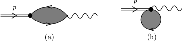
Figure 5: Two diagrams contributing to $g_{V\gamma}$.

Contribution of the diagram shown at Fig.5b looks as

$$\begin{split}\mathcal{M}_{\mu\nu}^{\mathrm{(b)}}&=Ch_{V}\sum_{n^{\prime}}\mathcal{O}_{n^{\prime}0}(p^{2})\int d\sigma\mathrm{Tr}S(x,x)V^{n^{\prime}}_{A}(x)\gamma_{\mu}\\ &=Ch_{V}\sum_{n^{\prime}}\mathcal{O}_{n^{\prime}0}(p^{2})\mathrm{Tr}_{v}\frac{v}{8\pi^{2}}\int_{0}^{1}ds\int_{0}^{1}d\tau\int_{\varepsilon}^{1}dt\left(\frac{1-s}{1+s}\right)^{m_{f}^{2}/4v\Lambda^{2}}t^{n^{\prime}}\frac{\partial^{n^{\prime}}}{\partial t^{n^{\prime}}}\frac{1}{\Phi_{5}^{2}}\left[\delta_{\mu\nu}\Phi_{6}-p_{\mu}p_{\nu}\Phi_{7}\right]\exp\left(-\frac{p^{2}}{4v}\Phi_{8}\right),\end{split}$$

$$\Phi_{5}=s+2tv,\quad\Phi_{6}=\frac{8tv}{s+2tv}=2-\frac{2s-4tv}{s+2tv},\quad\Phi_{7}=4st^{2}\tau^{2}v,\quad\Phi_{8}=\frac{st\tau^{2}v}{s+2tv}.$$

Form factors $I^{\mathrm{(a)}}_{\bot}$ and $I^{\mathrm{(b)}}_{\bot}$ contain divergences that cancel each other, so $I^{\mathrm{(a)}}_{\bot}+I^{\mathrm{(b)}}_{\bot}$ is finite after removal of regularization $\varepsilon\to 0$. Let us demonstrate this for ground state $n=0$:

$$I^{\mathrm{(a)}}_{\bot}+I^{\mathrm{(b)}}_{\bot}=\left(I^{\mathrm{(a)}}_{\bot}+\mathrm{Tr}_{v}\frac{1}{16\pi^{2}}\int_{0}^{1}ds_{1}\int_{0}^{1}ds_{2}\int_{\varepsilon}^{1}dt\frac{8v}{(s_{1}+s_{2}+2vt_{1})^{3}}\right)+\\ \left(I^{\mathrm{(b)}}_{\bot}-\mathrm{Tr}_{v}\frac{v}{8\pi^{2}}\int_{0}^{1}ds_{1}\int_{0}^{1}ds_{2}\int_{\varepsilon}^{1}dt\left[\frac{2}{(s+2vt)^{2}}-\frac{2s-4vt}{(s+2vt)^{3}}\right]\right)+\\ \mathrm{Tr}_{v}\left[-\frac{1}{16\pi^{2}}\int_{0}^{1}ds_{1}\int_{0}^{1}ds_{2}\int_{\varepsilon}^{1}dt\frac{8v}{(s_{1}+s_{2}+2vt_{1})^{3}}+\frac{v}{8\pi^{2}}\int_{0}^{1}ds_{1}\int_{0}^{1}ds_{2}\int_{\varepsilon}^{1}dt\frac{2}{(s+2vt)^{2}}\right]\\ -\mathrm{Tr}_{v}\frac{v}{8\pi^{2}}\int_{0}^{1}ds_{1}\int_{0}^{1}ds_{2}\int_{\varepsilon}^{1}dt\frac{2s-4vt}{(s+2vt)^{3}}.$$ (26)

Terms in round parentheses are finite in the limit $\varepsilon\to 0$. Terms in square brackets read

$$-\frac{1}{16\pi^{2}}\int_{0}^{1}ds_{1}\int_{0}^{1}ds_{2}\int_{\varepsilon}^{1}dt\frac{8v}{(s_{1}+s_{2}+2vt_{1})^{3}}+\frac{v}{8\pi^{2}}\int_{0}^{1}ds_{1}\int_{0}^{1}ds_{2}\int_{\varepsilon}^{1}dt\frac{2}{(s+2vt)^{2}}=\\ \frac{v}{4\pi^{2}}\left(\frac{1}{2v}\ln\frac{\varepsilon(1+2v)^{2}(1+\varepsilon v)}{(1+v)(1+2\varepsilon v)^{2}}-\frac{1}{2v}\ln\frac{\varepsilon(1+2v)}{1+2\varepsilon v}\right)=\\ \frac{1}{8\pi^{2}}\ln\frac{(1+2v)(1+\varepsilon v)}{(1+v)(1+2\varepsilon v)}\xrightarrow{\varepsilon\to 0}\frac{1}{8\pi^{2}}\ln\frac{1+2v}{1+v}.$$

The limit $\varepsilon\to 0$ of the last term in Eq.(26) reads

$$-\mathrm{Tr}_{v}\frac{v}{8\pi^{2}}\int_{0}^{1}ds_{1}\int_{0}^{1}ds_{2}\int_{\varepsilon}^{1}dt\frac{2s-4vt}{(s+2vt)^{3}}=\frac{v}{4\pi^{2}}\frac{1-\varepsilon}{(1+2v)(1+2\varepsilon v)}\xrightarrow{\varepsilon\to 0}\frac{v}{4\pi^{2}}\frac{1}{1+2v}.$$

Gauge invariance requirement

$$I^{\mathrm{(a)}}_{\|}+I^{\mathrm{(b)}}_{\|}=0$$

holds, which has been checked numerically.

Table 5: Decay and transition constants of various mesons

Meson	$n$	$f_{P}^{\rm exp}$	$f_{P}$	Meson	$n$	$g_{V\gamma}$ PDG	$g_{V\gamma}$
		(MeV)	(MeV)
$\pi$	0	130 PDG	140	$\rho$	0	0.2	0.2
$\pi(1300)$	1		29	$\rho$	1		0.053
$K$	0	156 PDG	175	$\omega$	0	0.059	0.067
$K(1460)$	1		27	$\omega$	1		0.018
$D$	0	205 PDG	212	$\phi$	0	0.074	0.071
$D$	1		51	$\phi$	1		0.02
$D_{s}$	0	258 PDG	274	$J/\psi$	0	0.09	0.06
$D_{s}$	1		57	$J/\psi$	1		0.015
$B$	0	191 PDG	187	$\Upsilon$	0	0.025	0.014
$B$	1		55	$\Upsilon$	1		0.0019
$B_{s}$	0	253 Chiu:2007bc	248
$B_{s}$	1		68
$B_{c}$	0	489 Chiu:2007bc	434
$B_{c}$	1		135

Numerical values of transition constants are given in Table 5. Though the masses of $\rho$ and $\omega$ mesons are equal to each other, their transition constants $g_{V\gamma}$ differ due to isospin. Transition constants $g_{V\gamma}$ for heavy quarkonia turn out to be underestimated. Though a clear reason for this has not been identified yet, it could be due to the necessity to take into account larger $N$ in calculations related to heavy quarkonia.

IV.3 Leptonic decay constants

Leptonic decay constant is defined as

$$M(P_{n}\rightarrow l\overline{\nu})=i\frac{G_{F}}{\sqrt{2}}\mathcal{K}F_{n}\left(p^{2}\right)\Phi_{P}(k)k_{\mu}\overline{l}(k^{\prime})\gamma_{\mu}(1-\gamma_{5})\nu(k+k^{\prime}),$$

$$f_{P_{n}}=F_{n}\left(-M^{2}_{n}\right),$$

where $\mathcal{K}$ is CKM matrix element corresponding to a given meson.

The contributions to $F_{n}$ of diagrams (a) and (b) shown in Fig. 6 are given by the formulas

$$F^{(a)}_{n}(p^{2})=h_{P_{n}}\sum_{n^{\prime}}\mathcal{O}_{n^{\prime}n}(p^{2})\int d\sigma\int\frac{d^{4}p^{\prime}}{2\pi^{4}}\int d^{4}xe^{ipx}\int d^{4}ye^{ip^{\prime}y}\mathrm{Tr}S_{f}(y,x)V^{n^{\prime}}(x)S_{f^{\prime}}(x,y)\gamma_{\mu}(1-\gamma_{5})$$

$$F^{(b)}_{n}(p^{2})=h_{P_{n}}\sum_{n^{\prime}}\mathcal{O}_{n^{\prime}n}(p^{2})\int d\sigma\frac{1}{\mathcal{K}}\sum_{f}\mathrm{Tr}S_{f}(x,x)V^{n^{\prime}}_{Wff}(x)$$

$\mathcal{O}_{nn^{\prime}}$ is the matrix that diagonalizes polarization operator $\tilde{\Pi}^{nn^{\prime}}_{P}$ corresponding to meson under consideration. After standard calculations one obtains the following expression for $f_{P_{n}}$

$$f_{P_{n}}=h_{P_{n}}\sum_{n^{\prime}}\mathcal{O}_{n^{\prime}n}(-M_{n}^{2})\frac{1}{4\pi^{2}}\left\{\mathrm{Tr}_{v}\int_{0}^{1}\!\int_{0}^{1}\!\int_{0}^{1}\!dtds_{1}ds_{2}\left(\frac{1-s_{1}}{1+s_{1}}\right)^{m_{f_{1}}^{2}/4v\Lambda^{2}}\left(\frac{1-s_{2}}{1+s_{2}}\right)^{m_{f_{2}}^{2}/4v\Lambda^{2}}\right.$$

$$\times t^{n^{\prime}}\frac{\partial^{n^{\prime}}}{\partial t^{n^{\prime}}}\frac{1+s_{1}s_{2}}{(s_{1}+s_{2}+2(1+s_{1}s_{2})tv)^{3}}\left(m_{f_{1}}\frac{s_{1}+2tv\left(1-\xi_{1}\left(1+s_{1}^{2}\right)\right)}{1-s_{1}^{2}}+m_{f_{2}}\frac{s_{2}+2tv\left(1-\xi_{2}\left(1+s_{2}^{2}\right)\right)}{1-s_{2}^{2}}\right)$$

$$\times\exp\left({\frac{M_{Pn}^{2}}{2v\Lambda^{2}}\frac{s_{1}s_{2}+2\left(\xi_{1}^{2}s_{1}+\xi_{2}^{2}s_{2}\right)tv}{s_{1}+s_{2}+2(1+s_{1}s_{2})tv}}\right)-$$

$$-2\xi_{1}m_{f_{1}}\mathrm{Tr}_{v}\int_{0}^{1}\int_{0}^{1}\int_{0}^{1}dsdtd\tau\left(\frac{1-s}{1+s}\right)^{m_{f_{1}}^{2}/4v\Lambda^{2}}t^{n^{\prime}}\frac{\partial^{n^{\prime}}}{\partial t^{n^{\prime}}}\frac{vst\tau}{(s+2vt)^{3}}\exp\left(\frac{M_{Pn}^{2}}{\Lambda^{2}}\frac{\xi_{1}^{2}st\tau^{2}}{s+2vt}\right)$$

$$\left.-2\xi_{2}m_{f_{2}}\mathrm{Tr}_{v}\int_{0}^{1}\int_{0}^{1}\int_{0}^{1}dsdtd\tau\left(\frac{1-s}{1+s}\right)^{m_{f_{2}}^{2}/4v\Lambda^{2}}t^{n^{\prime}}\frac{\partial^{n^{\prime}}}{\partial t^{n^{\prime}}}\frac{vst\tau}{(s+2vt)^{3}}\exp\left(\frac{M_{Pn}^{2}}{\Lambda^{2}}\frac{\xi_{2}^{2}st\tau^{2}}{s+2vt}\right)\right\}.$$ (27)

Numerical values of several leptonic decay constants are given in Table 5. In agreement with general expectations based on arguments related to the chiral symmetry breaking Holl:2004fr and finite energy sum rules krasnikov ; kataev , decay constants are order of magnitude smaller for excited states than for the ground state mesons. In the present approach this sharp decrease is a highly nontrivial feature since the integrand in (27) includes exponents of $M_{Pn}^{2}/\Lambda^{2}\sim 10$, and naively one would expect large decay constants. However, the chiral symmetry realisation combined with the orthogonal transformation $\mathcal{O}$ correctly leads to very small value.

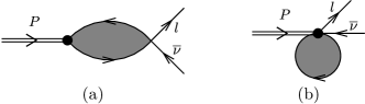
Figure 6: Two diagrams contributing to $f_{P}$.

V Discussion

In this section we touch on several issues which have not been fully elaborated yet but appear to be very important as they allow one to identify the place of the present approach among other models of confinement, chiral symmetry breakdown and hadronization as well as the methods underlining them. These are potential interrelations of the present approach to the soft wall AdS/QCD models, comparison of the properties of gluon correlator (8) with the Landau gauge gluon and quark propagators as they appear in functional renormalization group, Schwinger-Dyson Equations and lattice QCD, as well as details of chiral symmetry realization in the present approach. Some basic properties of these approaches seem to be visible from the viewpoint of the present formalism.

V.1 AdS/QCD and harmonic confinement

Bosonization of the four-quark interaction (6) in terms of bilocal meson-like fields $\Phi_{Jc}(x,z)$ leads to the following quadratic part of the effective action

$$\mathcal{S}_{2}=-\frac{1}{2}\int d^{4}x\int d^{4}zD(z)\Phi^{2}_{Jc}(x,z)$$

$$-2g^{2}\int d^{4}xd^{4}x^{\prime}d^{4}zd^{4}z^{\prime}D(z)D(z^{\prime})\Phi_{Jc}(x,z)\Pi_{Jc,J^{\prime}c^{\prime}}(x,x^{\prime};z,z^{\prime})\Phi_{J^{\prime}c^{\prime}}(x^{\prime},z^{\prime}),$$

$$\Pi_{Jc,J^{\prime}c^{\prime}}(x,x^{\prime};z,z^{\prime})={\rm Tr}V_{Jc}(x,z)S(x,x^{\prime})V_{J^{\prime}c^{\prime}}(x^{\prime},z^{\prime})S(x^{\prime},x),$$

$$V_{Jc}(x,z)=\Gamma_{J}t_{c}\exp\left\{iz_{\mu}\stackrel{{\scriptstyle\leftrightarrow}}{{\mathcal{D}}}_{\mu}(x)\right\}.$$ (28)

Meson eigenfunctions $f^{nl}_{\mu_{1}\dots\mu_{l}}(z)$ in the decomposition

$$\Phi^{aJ}(x,z)=\sum_{nl}\left(z^{2}\right)^{l/2}f^{nl}_{\mu_{1}\dots\mu_{l}}(z)\Phi^{aJln}_{\mu_{1}\dots\mu_{l}}(x)$$

are defined by the action $S_{2}$ via corresponding integral equation. Solution of this eigenfunction problem is equivalent to diagonalization of the quadratic part of the effective action in Eq.(14). Specific Gaussian form (7) of gluon propagator $D(z)$ is the reason for the radial part of the wave functions to be represented in terms of the generalized Laguerre polynomials, see Eq. (11). The mass spectrum has Regge character EN .

For the quadratic in $z$ dilaton profile $\varphi(z)=\kappa z^{2}$ soft wall AdS/QCD models arrive at the decomposition

$$\Phi_{j}(x,z)=\sum_{n}\phi_{nj}(z)\Phi_{nJ}(x)$$

with the radial meson wave functions proportional to generalized Laguerre polynomials,

$$\phi_{nj}=R^{j-3/2}\kappa^{1+l}z^{l-j+2}L^{l}_{n}(\kappa^{2}z^{2}),$$

which is a solution of the eigenfunction problem in differential form. The eigenvalues can be treated as the meson masses squared, and they strictly correspond to Regge spectrum for the quadratic in $z$ dilaton field.

There are obvious differences between effective action (28) and the soft wall AdS/QCD action. The fifth space-time coordinate $z$ of AdS/QCD model appears in the present approach as a distance between quark and anti-quark. There are four $z$-coordinates in (28), and hence the meson wave function contains angular part. Also it is not immediately clear where AdS metrics could come from in Eq.(28). Apart from this, the feature in common is the Gaussian weight function which in both cases plays the most important role for Regge character of the mass spectrum. After integrating out $z$ coordinate the quadratic part of the effective meson action put on-shell (that is neglecting terms of order $(p^{2}-M^{2})^{k}$ with $k\geq 2$),

$$\mathcal{S}_{2}=\frac{1}{2}\sum_{aJln}\int d^{4}x\tilde{\phi}_{aJln}(-p)\left(p^{2}-M^{2}_{aJln}\right)\tilde{\phi}_{aJln}(p),$$

is equivalent to the effective actions constructed within the AdS/QCD models.

One gets an impression that the form of dilaton profile in soft wall AdS/QCD approach could be linked to the gluon propagator and thus to the properties of QCD vacuum. A systematic verification of this conjecture requires derivation of the approximate (or reduced to some appropriate limit) differential form of the action (28). Weight and basis functions of the domain model have to be systematically compared with those employed in soft-wall AdS/QCD Karch:2006pv and harmonic confinement Leutwyler:1977vz ; Leutwyler:1977vy ; Leutwyler:1977pv ; Leutwyler:1977cs ; Leutwyler:1978uk approaches.

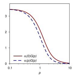
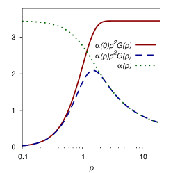
Figure 7: Momentum dependence of the gluon propagator (LHS plot) and dressing function (RHS plot) without (solid line) and with (dashed line) accounting for the running of the strong coupling constant $\alpha_{s}(p)$ (dotted line) modelled by the function (29). The dashed line reproduces the shape of the Landau gauge dressing function of gluons calculated within functional renormalization group Jan2015 and Lattice QCD Bowman ; Ilgenfritz as well as a part of the input gluon propagator used in the approaches based on combined Dyson-Schwinger and Bethe-Salpeter equations Maris ; Fischer:2014xha ; Dorkin:2014lxa .

V.2 Gluon propagator: Landau gauge DSE, FRG, LQCD vs Abelian (anti-)self-dial field

It is interesting to take a look at the properties of gluon (8) and quark (III) correlators in view of the known functional form of quark and Landau gauge gluon propagators calculated within the functional renormalization group, Lattice QCD and Dyson-Schwinger equations Bowman ; Ilgenfritz ; Jan2015 ; Maris ; Fischer:2014xha ; Dorkin:2014lxa . We do not intend to compare the propagators on a detailed quantitative basis if for no other reason than difference in gauge condition. Unlike just mentioned studies, the present approach have assumed background gauge condition so as renormalization of quark-gluon coupling constant is related to the gluon field renormalization. The tree level gluon propagator (8) without radiative corrections multiplied by the IR limit of the running coupling constant $\alpha_{s}(0)$ and corresponding ”dressing” function are shown by solid lines in Fig.7. At large Euclidean momenta the propagator (solid line in LHS of Fig.7) behaves as the free one ($1/p^{2}$) and the dressing function approaches to a constant value (solid line in RHS of Fig.7). In order to model the logarithmic scaling at short distances, one may divide the tree-level propagator by an appropriate logarithm, which, for background gauge, can be attributed to the effective running coupling constant,

$$\alpha_{s}(p)G(p)=\frac{\alpha_{s}(p)}{p^{2}}\left(1-e^{-p^{2}/\Lambda^{2}}\right),\ \ \alpha_{s}(p)=\alpha_{s}(0)Z(p),$$

$$Z(p)=\frac{12\pi}{11N_{\rm c}}\frac{1}{\ln(\zeta+p^{2}/\Lambda^{2})},\ \zeta=\exp\left(\frac{12\pi}{11N_{\rm c}}\right).$$ (29)

Here the form of logarithmic factor has been chosen to correspond to the form used in Maris ; Fischer:2014xha ; Dorkin:2014lxa . The result is shown by the dashed lines in Fig.7. One can see that the propagator itself (LHS) is not that much affected by taking into account the short distance scaling. On the contrary, the dressing function is expectedly modified at large $p^{2}$ (RHS). The shape of modified by logarithmic scaling gluon correlator is in agreement with the result of ab initio numerical calculations presented in Bowman ; Ilgenfritz ; Jan2015 and a corresponding part of ad-hoc postulated input gluon propagator for the quark DSE Maris ; Fischer:2014xha ; Dorkin:2014lxa . In the present set-up, the bump in the dressing function is due to the explicit $(1-\exp(-p^{2}/\Lambda^{2}))$ factor in the fluctuation gluon field propagator (8) in the presence of the Abelian (anti-)self-dual nonperturbative gluon fields. This factor is also responsible for the absence of a pole in the propagator which would correspond to the colour charged particles in the spectrum. In the infra-red limit the dressing function behaves as $p^{2}/\Lambda^{2}$, where scale $\Lambda$ is exactly the same for the tree level (solid line) and UV-corrected (dashed line) dressing functions in Fig.7. In our approach scale $\Lambda$, a gluon gap, is related to the scalar gluon condensate represented in terms of the Abelian (anti-)self-dual vacuum fields. It is also notable that identification of this gap with a kind of literally understood gluon mass would be misleading.

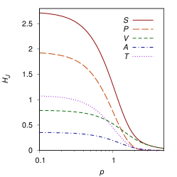
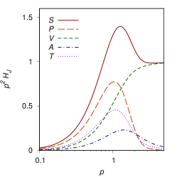
Figure 8: Momentum dependence of various form factors $\mathcal{H}_{J}$ entering the quark propagator (10) and corresponding dressing functions (RHS plot) for the case of constant quark mass ($m=145$MeV,  $\Lambda=415$MeV) . Dimensionless notations are used: $p^{2}=p^{2}/2v\Lambda^{2}$.

Figure 9: Schematically represented mass corrections to the quark propagator due to the constant scalar condensates $\Phi^{(0)}_{n}$ coupled to nonlocal form factor $F_{n0}$. Summation over the radial number $n$ is assumed.

V.3 Quark propagator, confinement and chiral symmetry: DSE vs scaling in the Abelian (anti-)self-dial background

Qualitative analysis of the scaling properties can be done with regard to the quark propagator. The tree level propagator (III) takes into account the background Abelian (anti-)self-dual field exactly and completely neglects perturbative radiative corrections. In this approximation the quark mass has a meaning of the IR limit of the effective running mass.

The propagator has complicated Dirac structure (10) which includes the complete set of Dirac matrices $\Gamma_{J}$ with corresponding form factors $\mathcal{H}_{J}(p^{2})$ ($J=S$, $P$, $V$, $A$, $T$). For the case of constant quark mass $m(0)$ functions $\mathcal{H}_{J}(p^{2})$ and corresponding dressing functions $p^{2}\mathcal{H}_{J}(p^{2})$ are shown in Fig.8. At large Euclidean momentum (short distance) the scalar and vector dressing functions tend to unity while the rest of functions vanish quickly, and the propagator approaches the free Dirac propagator with mass $m(0)$.

If one switches on the momentum dependence of the quark masses and naturally assumes that $m^{2}(p)\ll p^{2}$ at large momenta $p^{2}\gg 1$ (we use here dimensionless notation $p^{2}=p^{2}/2v\Lambda^{2}$, $m^{2}=m^{2}/2v\Lambda^{2}$ ) then the following simple asymptotic relations hold

$$\mathcal{H}_{V}=\int_{0}^{1}ds\left(\frac{1-s}{1+s}\right)^{m^{2}(p)/2}e^{-p^{2}s}\xrightarrow{p^{2}\to\infty}\frac{1}{p^{2}+m^{2}(p)}+O\left(e^{-p^{2}}\right),$$

$$\mathcal{H}_{A}=\int_{0}^{1}ds\left(\frac{1-s}{1+s}\right)^{m^{2}(p)/2}se^{-p^{2}s}\xrightarrow{p^{2}\to\infty}\frac{1}{(p^{2}+m^{2}(p))^{2}}+O\left(e^{-p^{2}}\right),$$

$$\mathcal{H}_{S}=\int_{0}^{1}ds\left(\frac{1-s}{1+s}\right)^{m^{2}(p)/2}\frac{1}{1-s^{2}}e^{-p^{2}s}\xrightarrow{p^{2}\to\infty}\frac{1}{p^{2}+m^{2}(p)}+\frac{e^{-p^{2}}}{m^{2}(p)}+O\left(e^{-p^{2}}\right),$$

$$\mathcal{H}_{P}=\int_{0}^{1}ds\left(\frac{1-s}{1+s}\right)^{m^{2}(p)/2}\frac{s^{2}}{1-s^{2}}e^{-p^{2}s}\xrightarrow{p^{2}\to\infty}\frac{2}{(p^{2}+m^{2}(p))^{3}}+\frac{e^{-p^{2}}}{m^{2}(p)}+O\left(e^{-p^{2}}\right),$$

$$\mathcal{H}_{T}=\frac{1}{2}\int_{0}^{1}ds\left(\frac{1-s}{1+s}\right)^{m^{2}(p)/2}\frac{s}{1-s^{2}}e^{-p^{2}s}\xrightarrow{p^{2}\to\infty}\frac{1}{2(p^{2}+m^{2}(p))^{2}}+\frac{e^{-p^{2}}}{2m^{2}(p)}+O\left(e^{-p^{2}}\right).$$

It should be stressed here that the first leading terms in above equations have the standard perturbative form while the subleading terms are purely nonperturbative, and they are suppressed by the Gaussian exponents. The squared mass in the denominator of subleading terms in the last three form factors ($J=S,P,T$) originate from the zero mode contribution to the propagator. These terms are also finite since the scaling of the mass to zero value (in the absence of the current masses!) is suppressed by the Gaussian factor if $m^{2}(p)>\exp(-p^{2})$ at asymptotically large $p^{2}$. In the limit $p^{2}\to\infty$ various dressing functions $p^{2}{\mathcal{H}}_{J}$ of the quark propagator read

$$p^{2}\mathcal{H}_{V}\to 1,\ p^{2}\mathcal{H}_{S}\to 1,\ p^{2}\mathcal{H}_{A}\to\frac{1}{p^{2}},\ p^{2}\mathcal{H}_{P}\to\frac{2}{(p^{2})^{2}},\ p^{2}\mathcal{H}_{T}\to\frac{1}{2p^{2}},$$

irrespective to the running of the quark mass. In particular, the scalar dressing function multiplied by the mass approaches the running quark mass,

$$m(p)\ p^{2}\mathcal{H}_{S}\to m(p)+\frac{e^{-p^{2}}}{m(p)}+O\left(m(p)e^{-p^{2}}\right).$$

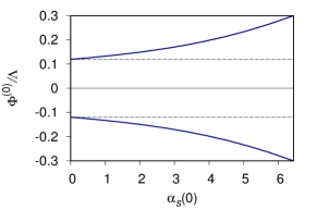
Figure 10: Scalar condensate $\Phi^{(0)}/\Lambda$ versus $\alpha_{s}(0)$ is given by solid lines, see Eq. (32).

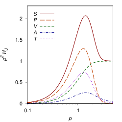
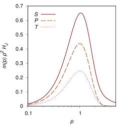
Figure 11: Momentum dependence of the scalar (solid line), pseudoscalar (long dash), vector (dash), axial (dash dot) and tensor (dot) dressing functions (LHS plot) in the quark propagator (10) and scalar, pseudoscalar and tensor dressing functions (RHS plot) multiplied by the quark mass for the case of the running mass $m(p)$ given in Eq.(31) ($m(0)=145$MeV,  $\Lambda=415$MeV). Dimensionless notation $p^{2}/2v\Lambda^{2}\to p^{2}$ is used.

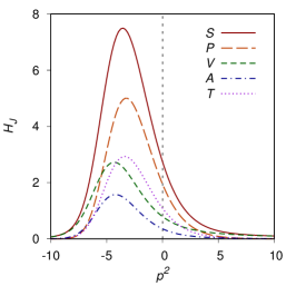
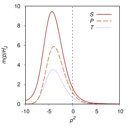
Figure 12: Momentum dependence of the scalar (solid line), pseudoscalar (long dash), vector (dash), axial (dash dot) and tensor (dot) form factors (LHS plot) in the quark propagator (10), and scalar, pseudoscalar and tensor form factors (RHS plot) multiplied by the quark mass for the case of the running mass $m(p)$ given in Eq.(31) with ($m(0)=145$MeV,  $\Lambda=415$MeV). Dimensionless notation $p^{2}/2v\Lambda^{2}\to p^{2}$ is used.

One can see that at large momenta the propagator approaches the standard Dirac propagator. For intermediate values of momenta the dressing functions are shown in LHS of Fig.11. The RHS of this figure emphasizes that the scalar part of the dressing function multiplied by the mass (see (10)) scales at large momentum as the running mass, while pseudoscalar and tensor structures vanish.

Equation (16) for scalar condensates $\Phi^{(0)}_{n0}$ suggests a verisimilar model for the nonperturbative running constituent mass of the quarks

$$m(p)=\bar{m}(0)\sum_{n=0}^{\infty}C_{n}F_{n0}\left(-\frac{p^{2}}{\Lambda^{2}}\right),$$ (30)

where we have returned to the dimensionful notation. The coefficients $C_{n}$ are normalized as

$$\sum_{n=0}^{\infty}C_{n}F_{n0}\left(0\right)=1.$$

If contributions to the quark mass corresponding to $n>0$ are neglected in Eq.(30) then the running mass in the chiral limit

$$m(p)=\bar{m}(0)F_{00}(p^{2}),\ \ F_{00}(p)=\left[1-\exp\left(-\frac{p^{2}}{\Lambda^{2}}\right)\right]\frac{\Lambda^{2}}{p^{2}},\ \ \bar{m}(0)=\frac{1}{3}g\Phi^{(0)},$$ (31)

is defined by the equation

$$\Phi^{(0)}-\frac{\alpha_{s}\Phi^{(0)}}{9\sqrt{2}\pi}\mathrm{Tr}_{v}\frac{1}{v}\int_{0}^{\infty}dp^{2}p^{2}F^{2}_{00}(p)\int_{0}^{1}ds\left(\frac{1-s}{1+s}\right)^{\frac{m^{2}(p)}{4v}}\frac{1}{1-s^{2}}\exp\left(-\frac{p^{2}}{2v}s\right)=0,$$ (32)

where we have used dimensionless notation

$$\frac{p^{2}}{\Lambda^{2}}\to p^{2},\quad\frac{m}{\Lambda}\to m,\quad\frac{\Phi_{0}}{\Lambda}\to\Phi_{0}.$$

As is illustrated in Fig.10 this equation has two solutions $\Phi_{0}(\alpha_{s})$ for any $\alpha_{s}$. The trivial solution $\Phi_{0}=0$ is absent as the integral over $s$ is singular in the limit $\Phi_{0}\to 0$ due to the contribution of zero modes. We see that there are two contributions to the scalar condensate: the vacuum field itself and the four-fermion interaction. Thus, due to the Abelian (anti-)self-dual vacuum field the chiral symmetry is spontaneously broken for arbitrarily small four-fermion interaction. For the values of strong coupling constant and scale given in the Table 1, $\alpha_{s}=3.45$ and $\Lambda=416$ MeV, one arrives at the estimate $\bar{m}(0)=166$ MeV, which is not that different from the value (25). It is also very important that the quark propagator with the running mass of the form (30) remains an entire analytical function in the complex $p^{2}$ plane, and the dynamical confinement property stays intact. Moreover, the propagator with the running mass decreases both in Euclidean and Minkowski domains of $p^{2}$, as it is illustrated in Fig.11. Similar shape of the scalar and vector form factors was reported in Dyson-Schwinger approach Souchlas:2010boa and interpreted in terms of the complex conjugated poles of the quark propagator. However this is not a unique interpretation, as one may conclude from the present consideration.

The full set of constants $\Phi_{n}^{(0)}$, which correspond to the invariant with respect to the local gauge transformation quark condensates $\langle\bar{\psi}(x)F_{n0}(\stackrel{{\scriptstyle\leftrightarrow}}{{\cal D}}(x)/\Lambda^{2})\psi(x)\rangle$, can be obtained by means of complete solution of Eq.(16) including heavy flavours. Like equation (32), in the chiral limit this system of equations is free from divergences, both ultraviolet and infrared (for discussion of analogous quark condensates see paper Dorokhov:2005pg ). Complete solution of Eq.(16) should allow us to use the current quark masses as free parameters instead of the infrared limit of the nonperturbative constituent masses.

VI Summary

In the present approach, dependence of the light meson masses on radial quantum number $n$ and orbital momentum $l$ has Regge character for $n\gg 1$ or $l\gg 1$ as it has been shown long time ago EN1 . The source of Regge mass spectrum in the model is the same as the source of dynamical colour confinement – the impact of the Abelian (anti-)self-dual background fields onto gluon and quark propagators resulting in the absence of singularities in propagators in the whole complex momentum plane. Gaussian exponential dependence of propagators on momentum is of particular importance for the strictly equidistant spectrum of $M_{nl}^{2}$ (see a highly instructive consideration of the toy nonlocal Kutkosky model in papers EG ; NKS ). Nondiagonal in radial number terms in the quadratic part of the action were neglected in our previous estimations EN ; NK4 . Results of improved computation with proper diagonalisation is given in Tables 2, 3, 4 and 5. Diagonalization significantly changes the values of parameters of the model but does not affect main features of the model. The values of parameters given in Table 1 were fitted to ground state mesons $\pi,\rho,K,K^{*},\eta^{\prime},J/\psi,\Upsilon$. The rest of masses, decay and transition constants were computed straightforwardly without further tuning of the parameters. In particular the same strong coupling constant was taken for light, heavy light mesons and heavy quarkonia. Diagonalization in combination with chiral symmetry implementation turned out to be crucial for computation of leptonic decay constants $f_{P}$ for radially excited states. In comparison with available experimental data the overall accuracy of the model is about 11-15% (with very few exceptions like $g_{V\gamma}$ for heavy quarkonia).

In the Discussion section we have touched on several important issues related to the chiral symmetry implementation, comparison with FRG and DSE results for propagators, and the interrelation of the present formalism with AdS/QCD models. More systematic study of these problems will be presented elsewhere.

Appendix A $U(1)$-gauging of the nonlocal meson action

Let us start with the generating functional

$$Z=\int d\sigma_{\mathrm{vac}}D\bar{q}Dq\exp\left\{-\int\!\!\!\int d^{4}xd^{4}y\bar{q}_{f}(x)S_{f}^{-1}(x,y|B)q_{f}(y)\right.\\ \left.+g^{2}\sum_{aJ}C_{J}\int\!\!\!\int d^{4}xd^{4}yD(y|\Lambda^{2})J^{\dagger aJ}(x,y)J^{aJ}(x,y)\right\}.$$

Bilocal currents $J^{aJ}(x,y)$ are

$$J^{aJ}(x,y)=\bar{q}_{f}(x+\xi y)M_{ff^{\prime}}^{a}\Gamma^{J}\exp\left[-i\int_{x+\xi y}^{x-\xi^{\prime}y}dz_{\mu}\widehat{B}_{\mu}(z)\right]q_{f^{\prime}}(x-\xi^{\prime}y)$$

$$\xi=\frac{m_{f^{\prime}}}{m_{f}+m_{f^{\prime}}},\quad\xi^{\prime}=\frac{m_{f}}{m_{f}+m_{f^{\prime}}}.$$

To make the Lagrangian gauge invariant, one performs substitution

$$\partial_{\mu}\rightarrow\partial_{\mu}-ie_{f}A_{\mu}(x)$$

and insert the term Terning:1991yt

$$\exp\left[-ie_{f}\int_{x+\xi y}^{x}dz_{\mu}A_{\mu}(z)-ie_{f^{\prime}}\int_{x}^{x-\xi^{\prime}y}dz_{\mu}A_{\mu}(z)\right]$$

in $J^{aJ}(x,y)$. Bilocal current takes the form

$$J^{aJ}(x,y|A)=\bar{q}_{f}(x+\xi y)M_{ff^{\prime}}^{a}\Gamma^{J}\\ \exp\left[-i\int_{x+\xi y}^{x-\xi^{\prime}y}dz_{\mu}\widehat{B}_{\mu}(z)-ie_{f}\int_{x+\xi y}^{x}dz_{\mu}A_{\mu}(z)-ie_{f^{\prime}}\int_{x}^{x-\xi^{\prime}y}dz_{\mu}A_{\mu}(z)\right]q_{f^{\prime}}(x-\xi^{\prime}y).$$

Expanding $J^{aJ}(x,y|A)$ in powers of electric charge $e$, one obtains

$$J^{aJ}(x,y|A)=J^{aJ}(x,y)\left(1-ie_{f}\int_{x+\xi y}^{x}dz_{\mu}A_{\mu}(z)-ie_{f^{\prime}}\int_{x}^{x-\xi^{\prime}y}dz_{\mu}A_{\mu}(z)+\dots\right).$$

Integrals may be evaluated along the straight line:

$$i\int_{x+\xi y}^{x-\xi^{\prime}y}dz_{\mu}\widehat{B}_{\mu}(z)=-\frac{i}{2}x_{\mu}\widehat{B}_{\mu\nu}y_{\nu},$$

$$\int_{a}^{b}dz_{\mu}A_{\mu}(z)=\int_{a}^{b}dz_{\mu}\int\frac{d^{4}p}{(2\pi)^{4}}\tilde{A}_{\mu}(p)e^{ipz}=\int\frac{d^{4}p}{(2\pi)^{4}}\tilde{A}_{\mu}(p)\int_{a}^{b}dz_{\mu}e^{ipz},$$

$$\int_{a}^{b}dz_{\mu}e^{ipz}=\int_{0}^{1}d\tau(b-a)_{\mu}e^{ip(a+\tau(b-a))}=e^{ipa}\int_{0}^{1}d\tau\frac{1}{i\tau}\frac{\partial}{\partial p_{\mu}}e^{ip\tau(b-a)},$$

$$\int_{x+\xi y}^{x}dz_{\mu}A_{\mu}(z)=-\int^{x+\xi y}_{x}dz_{\mu}A_{\mu}(z)=-\int\frac{d^{4}p}{(2\pi)^{4}}\tilde{A}_{\mu}(p)e^{ipx}\int_{0}^{1}d\tau\frac{1}{i\tau}\frac{\partial}{\partial p_{\mu}}e^{ip\tau\xi y},$$

$$\int_{x}^{x-\xi^{\prime}y}dz_{\mu}A_{\mu}(z)=\int\frac{d^{4}p}{(2\pi)^{4}}\tilde{A}_{\mu}(p)e^{ipx}\int_{0}^{1}d\tau\frac{1}{i\tau}\frac{\partial}{\partial p_{\mu}}e^{ip\tau(-\xi^{\prime}y)}.$$

Expansion of the bilocal current up to the first power in charge may be rewritten as

$$J^{aJ}(x,y|A)=J^{aJ}(x,y)\left(1+\int\frac{d^{4}p}{(2\pi)^{4}}\tilde{A}_{\mu}(p)e^{ipx}\int_{0}^{1}d\tau\frac{1}{i\tau}\frac{\partial}{\partial p_{\mu}}\left\{ie_{f}e^{ip\tau\xi y}-ie_{f^{\prime}}e^{ip\tau(-\xi^{\prime}y)}\right\}+\dots\right).$$ (33)

Now variable $y$ may be integrated out:

$$V^{aJln}_{A}(x)=\int_{0}^{1}d\tau\frac{1}{\tau}\frac{\partial}{\partial p_{\mu}}\left\{e_{f}V^{aJln}\left(\stackrel{{\scriptstyle\leftrightarrow}}{{\nabla}}(x)+ip\tau\xi\right)-e_{f^{\prime}}V^{aJln}\left(\stackrel{{\scriptstyle\leftrightarrow}}{{\nabla}}(x)-ip\tau\xi^{\prime}\right)\right\}.$$ (34)

For example, the interaction of a ground-state meson with quark current and electromagnetic field is described by the vertex

$$V^{aJ00}_{A}=M_{ff^{\prime}}^{a}\Gamma^{J}\int_{0}^{1}d\tau\frac{1}{\tau}\frac{\partial}{\partial p_{\mu}}\int_{0}^{1}dt\left\{e_{f}\exp\left[\frac{t}{\Lambda^{2}}\left(\stackrel{{\scriptstyle\leftrightarrow}}{{\nabla}}+ip\tau\xi\right)^{2}\right]-e_{f^{\prime}}\exp\left[\frac{t}{\Lambda^{2}}\left(\stackrel{{\scriptstyle\leftrightarrow}}{{\cal D}}-ip\tau\xi^{\prime}\right)^{2}\right]\right\},$$

where $p$ is momentum of electromagnetic field.

Appendix B $SU(2)_{\mathrm{L}}\times U(1)_{\mathrm{Y}}$-gauging of the meson Lagrangian

Quark fields

$$Q=\left(u,c,t,d,s,b\right)^{\mathrm{T}}$$

that diagonalize mass matrix and Higgs interaction are transformed as

$$Q^{\omega,\varepsilon}=\exp\left(\begin{array}[]{cc}ig\omega^{3}T^{3}_{u}+ig^{\prime}Y_{L}\varepsilon&igV\frac{\omega^{1}-i\omega^{2}}{2}\\ igV^{\dagger}\frac{\omega^{1}+i\omega^{2}}{2}&ig\omega^{3}T^{3}_{d}+ig^{\prime}Y_{L}\varepsilon\end{array}\right)Q_{L}+\exp\left(\begin{array}[]{ccc}ig^{\prime}Q_{u}\varepsilon&0\\ 0&ig^{\prime}Q_{d}\varepsilon\end{array}\right)Q_{R}$$

under the action of $SU(2)_{\mathrm{L}}\times U(1)_{\mathrm{Y}}$, where $V$ is CKM matrix. The following notations are employed:

$$L=\frac{1-\gamma_{5}}{2},\quad R=\frac{1+\gamma_{5}}{2},\quad t^{a}=\frac{\sigma^{a}}{2},$$

$$Y_{L}=\frac{1}{6},\quad Y_{R}=\left(\begin{array}[]{cc}\frac{2}{3}&0\\ 0&-\frac{1}{3}\end{array}\right)=\left(\begin{array}[]{cc}Q_{u}&0\\ 0&Q_{d}\end{array}\right),\quad t^{3}=\left(\begin{array}[]{cc}\frac{1}{2}&0\\ 0&-\frac{1}{2}\end{array}\right)=\left(\begin{array}[]{cc}T^{3}_{u}&0\\ 0&T^{3}_{d}\end{array}\right),\quad t^{3}+Y_{L}=\left(\begin{array}[]{cc}Q_{u}&0\\ 0&Q_{d}\end{array}\right).$$

To provide gauge invariance of Lagrangian, bilocal current

$$J^{aJ}(x,y)=\bar{Q}_{f}(x+\xi y)M_{ff^{\prime}}^{a}\Gamma^{J}\exp\left[-i\int_{x+\xi y}^{x-\xi^{\prime}y}dz_{\mu}\widehat{G}_{\mu}(z)\right]Q_{f^{\prime}}(x-\xi^{\prime}y)=\\ \left(\bar{Q}_{fL}(x+\xi y)+\bar{Q}_{fR}(x+\xi y)\right)M_{ff^{\prime}}^{a}\Gamma^{J}\exp\left[-i\int_{x+\xi y}^{x-\xi^{\prime}y}dz_{\mu}\widehat{G}_{\mu}(z)\right]\left(Q_{f^{\prime}L}(x-\xi^{\prime}y)+Q_{f^{\prime}R}(x-\xi^{\prime}y)\right)$$

is modified in the following way:

$$\begin{split}J^{aJ}(x,y)\to\left\{\bar{Q}_{L}(x+\xi y)P\exp\left[\int_{x+\xi y}^{x}dz_{\mu}\left(\begin{array}[]{cc}-ieQ_{u}A_{\mu}-ig\frac{T^{3}_{u}-\sin^{2}\theta_{W}Y_{L}}{\cos\theta_{W}}Z_{\mu}&-i\frac{g}{\sqrt{2}}VW^{+}_{\mu}\\ -i\frac{g}{\sqrt{2}}V^{\dagger}W^{-}_{\mu}&-ieQ_{d}A_{\mu}-ig\frac{T^{3}_{d}-\sin^{2}\theta_{W}Y_{L}}{\cos\theta_{W}}Z_{\mu}\end{array}\right)\right]\right.+\\ \left.\bar{Q}_{R}(x+\xi y)\exp\left[\int_{x+\xi y}^{x}dz_{\mu}\left(\begin{array}[]{cc}-ieQ_{u}A_{\mu}+ig\frac{\sin^{2}\theta_{W}}{\cos\theta_{W}}Q_{u}Z_{\mu}&0\\ 0&-ieQ_{d}A_{\mu}+ig\frac{\sin^{2}\theta_{W}}{\cos\theta_{W}}Q_{d}Z_{\mu}\end{array}\right)\right]\right\}_{f}\\ \times M_{ff^{\prime}}^{a}\Gamma^{J}\exp\left[-i\int_{x+\xi y}^{x-\xi^{\prime}y}dz_{\mu}\widehat{G}_{\mu}(z)\right]\times\\ \left\{P\exp\left[\int^{x-\xi^{\prime}y}_{x}dz_{\mu}\left(\begin{array}[]{cc}-ieQ_{u}A_{\mu}-ig\frac{T^{3}_{u}-\sin^{2}\theta_{W}Y_{L}}{\cos\theta_{W}}Z_{\mu}&-i\frac{g}{\sqrt{2}}VW^{+}_{\mu}\\ -i\frac{g}{\sqrt{2}}V^{\dagger}W^{-}_{\mu}&-ieQ_{d}A_{\mu}-ig\frac{T^{3}_{d}-\sin^{2}\theta_{W}Y_{L}}{\cos\theta_{W}}Z_{\mu}\end{array}\right)\right]Q_{L}(x-\xi^{\prime}y)\right.+\\ \left.\exp\left[\int^{x-\xi^{\prime}y}_{x}dz_{\mu}\left(\begin{array}[]{cc}-ieQ_{u}A_{\mu}+ig\frac{\sin^{2}\theta_{W}}{\cos\theta_{W}}Q_{u}Z_{\mu}&0\\ 0&-ieQ_{d}A_{\mu}+ig\frac{\sin^{2}\theta_{W}}{\cos\theta_{W}}Q_{d}Z_{\mu}\end{array}\right)\right]Q_{R}(x-\xi^{\prime}y)\right\}_{f^{\prime}},\end{split}$$

$$W^{\pm}_{\mu}=\frac{W^{1}_{\mu}\mp iW^{2}_{\mu}}{\sqrt{2}},\quad A_{\mu}=\frac{g^{\prime}W^{3}_{\mu}+gB_{\mu}}{\sqrt{g^{2}+g^{\prime 2}}},\quad Z_{\mu}=\frac{gW^{3}_{\mu}-g^{\prime}B_{\mu}}{\sqrt{g^{2}+g^{\prime 2}}},$$

$$e=\frac{gg^{\prime}}{\sqrt{g^{2}+g^{\prime 2}}},\quad\cos\theta_{W}=\frac{g}{\sqrt{g^{2}+g^{\prime 2}}},\quad\sin\theta_{W}=\frac{g^{\prime}}{\sqrt{g^{2}+g^{\prime 2}}},$$

where $P$ is path-antiordering (higher values of path parameter stand to the right).

Now we are ready to investigate first-order perturbative expansion of the bilocal current. Let us consider an example of $W^{+}$ interaction with a charged meson. The term describing interaction of meson with quark current and $W^{+}$ is

$$\left\{\bar{Q}_{L}(x+\xi y)\int_{x+\xi y}^{x}dz_{\mu}\left(\begin{array}[]{cc}0&-i\frac{g}{\sqrt{2}}VW^{+}_{\mu}\\ 0&0\end{array}\right)\right\}_{f}M_{ff^{\prime}}^{a}\Gamma^{J}\exp\left[-i\int_{x+\xi y}^{x-\xi^{\prime}y}dz_{\mu}\widehat{G}_{\mu}(z)\right]Q_{f^{\prime}}(x+\xi^{\prime}y)+\\ \bar{Q}(x+\xi y)M_{ff^{\prime}}^{a}\Gamma^{J}\exp\left[-i\int_{x+\xi y}^{x-\xi^{\prime}y}dz_{\mu}\widehat{G}_{\mu}(z)\right]\left\{\int^{x-\xi^{\prime}y}_{x}dz_{\mu}\left(\begin{array}[]{cc}0&-i\frac{g}{\sqrt{2}}VW^{+}_{\mu}\\ 0&0\end{array}\right)Q_{L}(x-\xi^{\prime}y)\right\}_{f^{\prime}}=\\ -i\frac{g}{\sqrt{2}}\bar{Q}_{f_{1}}(x+\xi y)\exp\left[-i\int_{x+\xi y}^{x-\xi^{\prime}y}dz_{\mu}\widehat{G}_{\mu}(z)\right]\times\\ \left\{R\Gamma^{J}\left(\begin{array}[]{cc}0&V\\ 0&0\end{array}\right)_{f_{1}f}M_{ff^{\prime}}^{a}\delta_{f^{\prime}f_{2}}\int_{x+\xi y}^{x}dz_{\mu}W^{+}_{\mu}+\Gamma^{J}L\delta_{f_{1}f}M_{ff^{\prime}}^{a}\left(\begin{array}[]{cc}0&V\\ 0&0\end{array}\right)_{f^{\prime}f_{2}}\int^{x-\xi^{\prime}y}_{x}dz_{\mu}W^{+}_{\mu}\right\}Q_{f_{2}}(x-\xi^{\prime}y).$$

Proceeding in the way analogous to (33) and integrating out relative coordinate $y$, we write the desired vertex as

$$V^{aJln}_{W^{+}f_{1}f_{2}}=\frac{g}{\sqrt{2}}\int_{0}^{1}d\tau\frac{1}{\tau}\frac{\partial}{\partial p_{\mu}}\\ \left\{R\left(\begin{array}[]{cc}0&V\\ 0&0\end{array}\right)_{f_{1}f}V^{aJln}_{ff^{\prime}}\left(\stackrel{{\scriptstyle\leftrightarrow}}{{\cal D}}(x)+ip\tau\xi\right)\delta_{f^{\prime}f_{2}}-\delta_{f_{1}f}V^{aJln}_{ff^{\prime}}\left(\stackrel{{\scriptstyle\leftrightarrow}}{{\cal D}}(x)-ip\tau\xi^{\prime}\right)\left(\begin{array}[]{cc}0&V\\ 0&0\end{array}\right)_{f^{\prime}f_{2}}L\right\}.$$

References

- (1) R. P. Feynman, M, Kislinger, and F. Ravndal, Phys. Rev. D 3 (1971) 2706.
- (2) H. Leutwyler and J. Stern, Phys. Lett. B 73, 75 (1978).
- (3) H. Leutwyler and J. Stern, Annals Phys. 112, 94 (1978).
- (4) H. Leutwyler and J. Stern, Phys. Lett. B 69, 207 (1977).
- (5) H. Leutwyler and J. Stern, Nucl. Phys. B 133, 115 (1978).
- (6) H. Leutwyler and J. Stern, Nucl. Phys. B 157, 327 (1979).
- (7) A. Karch, E. Katz, D. T. Son and M. A. Stephanov, Phys. Rev. D 74, 015005 (2006) [hep-ph/0602229].
- (8) G. F. de Teramond and S. J. Brodsky, Phys. Rev. Lett. 94, 201601 (2005) [hep-th/0501022].
- (9) S. J. Brodsky and G. F. de Teramond, Phys. Rev. Lett. 96, 201601 (2006) [hep-ph/0602252].
- (10) G. F. de Teramond and S. J. Brodsky, Phys. Rev. Lett. 102, 081601 (2009) [arXiv:0809.4899 [hep-ph]].
- (11) R. Swarnkar and D. Chakrabarti, Phys. Rev. D 92, no. 7, 074023 (2015)
- (12) T. Gutsche, V. E. Lyubovitskij, I. Schmidt and A. Vega, Phys. Rev. D 91, 114001 (2015).
- (13) G.V. Efimov, and S.N. Nedelko, Phys. Rev. D 51, 176 (1995).
- (14) H. Leutwyler, Nucl. Phys. B 179 , 129 (1981).
- (15) H. Leutwyler, Phys. Lett. B 96, 154 (1980).
- (16) P. Minkowski, Phys. Lett. B 76, 439 (1978).
- (17) S. N. Nedelko and V. E. Voronin, Eur. Phys. J. A 51, 45 (2015).
- (18) H. Pagels, and E. Tomboulis, Nucl. Phys. B 143, 485 (1978).
- (19) A. Eichhorn, H. Gies and J. M. Pawlowski, Phys. Rev. D 83, 045014 (2011).
- (20) B.V. Galilo and S.N. Nedelko, Phys. Part. Nucl. Lett., 8, 67 (2011).
- (21) D. P. George, A. Ram, J. E. Thompson and R. R. Volkas, Phys. Rev. D 87, 105009 (2013). [arXiv:1203.1048 [hep-th]].
- (22) J. V. Burdanov, G. V. Efimov, S. N. Nedelko, S. A. Solunin, Phys. Rev. D 54, 4483 (1996).
- (23) A.C. Kalloniatis and S.N. Nedelko, Phys. Rev. D 64, 114025 (2001).
- (24) P. Olesen, Nucl. Phys. B 200, 381 (1982).
- (25) A.C. Kalloniatis and S.N. Nedelko, Phys. Rev. D 69, 074029 (2004).
- (26) L.D. Faddeev, arXiv:0911.1013 [math-ph].
- (27) A. C. Kalloniatis and S. N. Nedelko, Phys. Rev. D 73, 034006 (2006).
- (28) J. Praschifka, C. D. Roberts and R. T. Cahill, Phys. Rev. D 36, 209 (1987).
- (29) K.A. Olive et al. (Particle Data Group) Chinese Phys. C 38,090001 (2014).
- (30) Z. Dolezal [ATLAS Collaboration], PoS Bormio 2015, 035 (2015).
- (31) R. J. Dowdall, C. T. H. Davies, T. C. Hammant and R. R. Horgan, Phys. Rev. D 86, 094510 (2012) [arXiv:1207.5149 [hep-lat]].
- (32) T. W. Chiu et al. [TWQCD Collaboration], PoS LAT 2006, 180 (2007).
- (33) A. Holl, A. Krassnigg and C. D. Roberts, Phys. Rev. C 70, 042203 (2004).
- (34) A. L. Kataev, N. V. Krasnikov and A. A. Pivovarov, Phys. Lett. B 123, 93 (1983).
- (35) S. G. Gorishnii, A. L. Kataev and S. A. Larin, Phys. Lett. B 135, 457 (1984).
- (36) M. Mitter, J. M. Pawlowski and N. Strodthoff, Phys. Rev. D 91 (2015) 054035; [arXiv:1411.7978 [hep-ph]].
- (37) P. O. Bowman, U. M. Heller, D. B. Leinweber, M. B. Parappilly and A. G. Williams, Phys. Rev. D 70, (2004) 034509; [hep-lat/0402032].
- (38) A. Sternbeck, E.-M. Ilgenfritz, M. Muller-Preussker, A. Schiller and I. L. Bogolubsky, PoS LAT 2006, 076 (2006). [hep-lat/0610053].
- (39) P. Maris and P. C. Tandy, Phys. Rev. C 60, 055214 (1999)
- (40) C. S. Fischer, S. Kubrak and R. Williams, Eur. Phys. J. A 50, 126 (2014).
- (41) S. M. Dorkin, L. P. Kaptari and B. Kämpfer, Phys. Rev. C 91 (2015) 055201, arXiv:1412.3345 [hep-ph].
- (42) N. Souchlas, J. Phys. G 37,115001 (2010).
- (43) A. E. Dorokhov, Eur. Phys. J. C 42, 309 (2005).
- (44) G. V. Efimov and G. Ganbold, Phys. Rev. D 65, 054012 (2002).
- (45) A. C. Kalloniatis, S. N. Nedelko and L. von Smekal, Phys. Rev. D 70, 094037 (2004).
- (46) J. Terning, Phys. Rev. D 44, no. 3, 887 (1991).