Searching for a magnetic field in Wolf-Rayet stars using FORS 2 spectropolarimetry

Abstract

To investigate if magnetic fields are present in Wolf-Rayet stars, we selected a few stars in the Galaxy and one in the Large Magellanic Cloud (LMC). We acquired low-resolution spectropolarimetric observations with the ESO FORS 2 instrument during two different observing runs. During the first run in visitor mode, we observed the LMC Wolf-Rayet star BAT99 7 and the stars WR 6, WR 7, WR 18, and WR 23 in our Galaxy. The second run in service mode was focused on monitoring the star WR 6. Linear polarization was recorded immediately after the observations of circular polarization. During our visitor observing run, the magnetic field for the cyclically variable star WR 6 was measured at a significance level of 3.3$\sigma$ ($\left<B_{\rm z}\right>=258\pm 78$ G). Among the other targets, the highest value for the longitudinal magnetic field, $\left<B_{\rm z}\right>=327\pm 141$ G, was measured in the LMC star BAT99 7. Spectropolarimetric monitoring of the star WR 6 revealed a sinusoidal nature of the $\left<B_{\rm z}\right>$ variations with the known rotation period of 3.77 d, significantly adding to the confidence in the detection. The presence of the rotation-modulated magnetic variability is also indicated in our frequency periodogram. The reported field magnitude suffers from significant systematic uncertainties at the factor 2 level, in addition to the quoted statistical uncertainties, owing to the theoretical approach used to characterize it. Linear polarization measurements showed no line effect in the stars, apart from WR 6. BAT99 7, WR 7, and WR 23 do not show variability of the linear polarization over two nights.

1 Introduction

Magnetic fields are now believed to play an important role in the evolution of massive stars. A Tayler-Spruit dynamo mechanism (Spruit 2002) has been predicted to be efficient in radiative layers of the stellar interior. However, these fields perhaps do not reach the photosphere with a measurable strength. Cantiello et al. (2009) showed that subsurface convection zones may be present in massive stars. If a dynamo operates in such a zone, a magnetic field could emerge to produce observable phenomena such as magnetic spots or hot plasma close to the stellar surface (e.g., Waldron & Cassinelli 2007; Ramiaramanantsoa et al. 2014). Maeder & Meynet (2005) examined the effect of magnetic fields on the transport of angular momentum and chemical mixing, and found that the potential influence on the evolution of massive stars is drastic. Thus magnetic fields might change our whole picture about the evolution from O stars via Wolf-Rayet (WR) stars to supernovae/gamma-ray bursts. Hitherto, neglecting magnetic fields might be one of the reasons why models and observations of massive-star populations are still in conflict (Hamann et al. 2006). Another potential importance of magnetic fields in massive stars concerns the dynamics of the stellar winds. Wherever $B^{2}R^{2}_{*}>\dot{M}\varv_{\infty}$, it ushers a transition to magnetic control of the wind. If the field is weaker than this limit, the field lines are carried along with the wind of mass-loss rate $\dot{M}$ and (terminal) velocity $\varv_{\infty}$, and become more or less radial (e.g. ud-Doula & Owocki 2002).

Our long-standing interest is to understand WR stars in all their aspects, including their magnetic fields. Classical WR stars are massive stars that have lost their outer layers in a relatively short time. Thus, if a massive star has an interior dynamo as predicted by the Tayler-Spruit mechanism, the magnetized layers can now be displayed in the atmosphere with a field strength of many kG (Mullan & MacDonald 2005) or being even further condensed by the progressing stellar contraction.

There is indirect evidence, e.g. from spectral variability and X-ray emission, that magnetic fields are present in WR atmospheres (e.g. Michaux et al. 2014). Also the theoretical work of Gayley & Ignace (2010) predicts a degree of circular polarization of a few times 10^-4 for magnetic fields of about 100 G. The detection of magnetic fields is however difficult, chiefly because the line spectrum is formed in the strong stellar wind. This does not only imply a dilution of the field at the place of line formation. The big problem is the wind broadening of the emission lines by Doppler shifts with wind velocities of a few thousand km s^-1. In high-resolution spectropolarimetric observations, some broad spectral lines extend over adjacent orders, so that it is necessary to adopt the order shapes to get the best continuum normalization. In view of such immense line broadening in WR stars, to search for a weak magnetic field, we decided to use the low-resolution VLT instrument FORS 2 (FOcal Reducer low dispersion Spectrograph) mounted at the 8-m Antu telescope, which appears to be one of the most suitable instruments in the world offering low resolution and the required spectropolarimetric sensitivity.

Our sample of WR stars selected for the search of the presence of magnetic fields includes two rather bright WN4 stars, WR 6 and WR 18, and the WC6 star WR 23. Since the rotation period of WR 6 ($P_{\rm rot}=3.77$ d) was already determined and confirmed in the past by several teams (e.g., Lamontagne et al. 1986), one of our goals is to assess the presence of a magnetic field and its potential cyclical modulation over the rotation cycle, as expected for tilted dipole or split monopole geometries. Further, from our previous comprehensive analyses using the Potsdam Wolf-Rayet model atmospheres, we have identified a few Wolf-Rayet stars in the Galaxy and the Large Magellanic Cloud (LMC) that are in an extremely advanced stage of their evolution, being very compact ($R<\sim 2\,R_{\odot}$) and hot ($T_{\rm eff}>100$ kK). Having lost their outer layers, they now expose their cores and are promising targets to search for the presence of a magnetic field. The sample of Galactic WR stars with such very small stellar radii is very limited (cf. Hamann et al. 2006). Among them, WR 7 is the best candidate to be observed from the VLT observatory located on Cerro Paranal.

Additionally, probably for reasons of stellar evolution in the lower metallicity environment, the WN population in the LMC shows a higher fraction of very hot and compact WN stars (e.g., Hainich et al. 2014). We have chosen the brightest of these LMC objects, BAT99 7, as another target. BAT99 7 has an additional peculiarity that makes it an especially promising candidate for showing a strong magnetic field, which concerns the shape of its line profiles. These profile shapes are very round, unlike the Gaussian shape that is usually found in WR-type emission lines. We have found such type of line profiles in only two Galactic WR stars, but in five WN stars from the LMC. The reason for this profile shape is not clear. Model atmospheres are not able to reproduce it, unless one assumes broadening by extremely fast rotation. In the case of BAT99 7, we estimate a $v\,\sin\,i$ of 1900 km s^-1 to account for the profile shape when applying just flux convolution. Given the compactness of the star, such fast rotation is not impossible but close to the breakup limit, making these stars good GRB candidates. Rotational broadening may be enhanced by wind corotation enforced by a strong magnetic field, while the rotation itself can strengthen the dynamo.

WR 7 does not show such round line profiles, but is one of the few Wolf-Rayet stars that have been found to be X-ray active. The origin of X-rays from single-star winds is still under debate, and can be attributed either to wind shocks from the deshadowing instability (Gayley & Owocki 1995; Feldmeier et al. 1997), or Corotating Interaction Regions (CIRs) (Mullan 1984), or to magnetic effects (e.g., Waldron & Cassinelli 2009; Oskinova et al. 2009). BAT99 7 has not been seen in X-rays yet, but due to its large distance there is no tight upper limit either.

We note that a detailed quantitative spectral analysis of all stars in our sample was already carried out in previous studies (e.g., Hamann et al. 2006; Sander et al. 2012; Shenar et al. 2014). Any binary suspects are excluded from our target selection to avoid confusion between the magnetic field measurements and effects from colliding stellar winds.

In Section 2, we give an overview of our spectropolarimetric observations and the data reduction, followed by the presentation of the results of the magnetic field measurements for the individual stars in Section 3. Section 4 describes our measurement error validation using a synthetic spectrum and Section 5 is devoted to observations of the linear polarization. Finally, we summarize the results of our observations in Section 6.

2 Observations and data reduction

Table 1: Overview of the WR stars observed in the first run.

Object	Type	$m_{\rm V}$	Date
BAT99 7	WN4b	13.6	2010-12-23 and 24
WR 6	WN4	6.9	2010-12-24
WR 7	WN4	11.7	2010-12-23 and 24
WR 18	WN4	10.6	2010-12-24
WR 23	WC6	9.0	2010-12-23 and 24

The spectropolarimetric data presented in this paper were obtained with the FORS 2 instrument (Appenzeller et al. 1998) during two different observing runs. FORS 2 is a multi-mode instrument equipped with polarization analyzing optics, comprising super-achromatic half-wave and quarter-wave phase retarder plates, and a Wollaston prism with a beam divergence of 22$\arcsec$ in standard resolution mode. The first run took place in visitor mode during the two nights in 2010 December 23 and 24. During this run, the WR stars BAT99 7, WR 7, and WR 23 were observed twice and the stars WR 6 and WR 18 once. An overview of the observed targets during this visitor run including their types and visual magnitudes is presented in Table LABEL:tab:2010.

Table 2: Logbook of the FORS 2 circular polarization observations of WR 6, including the modified Julian date of mid-exposure followed by the rotation phase, the number of elapsed rotation cycles, and the achieved signal-to-noise ratio.

Date	MJD	$p$	Rotation	SNR
			cycle
2010 Dec. 24	55555.1577	0.560	$-$77	1353
2011 Oct. 10	55845.2716	0.596	0	1037
2011 Oct. 11	55846.2584	0.858	0	357
2011 Nov. 14	55880.1638	0.861	9	1139
2011 Dec. 7	55903.3172	0.009	15	1004
2011 Dec. 10	55906.1257	0.754	16	925
2011 Dec. 13	55909.2102	0.573	16	983
2012 Jan. 1	55928.0760	0.583	21	686
2012 Jan. 2	55929.0803	0.849	22	914
2012 Jan. 5	55932.0686	0.643	23	1141
2012 Jan. 6	55933.0511	0.904	23	1004
2012 Jan. 7	55934.0611	0.172	23	1235
2012 Jan. 8	55935.2491	0.487	23	1417

An examination of the data obtained during the first run revealed the strongest evidence for the presence of a magnetic field in the cyclically variable star WR 6, for which a photometric periodicity of 3.77 d was detected by Lamontagne et al. (1986). Motivated by this detection, we applied for a second observing run in service mode, consisting of twelve randomly distributed individual observations to sample the stellar rotation period. The detection of rotational modulation of the longitudinal magnetic field would constrain the global field geometry necessary to support physical modeling of the spectroscopic and light variations. The observing log of the service mode observations is presented in Table LABEL:tab:phase, together with the rotation phases, the elapsed rotation cycles and the signal-to-noise ratio (SNR) in the continuum. The rotation cycle 0 was assumed to begin at the start of our monitoring of WR 6 in service mode, i.e. on 2011 October 10. As the spectra of WR stars are dominated by wind emission lines, with the strongest emission appearing in the line He ii $\lambda$4686, special care was taken not to saturate this line with the achieved SNR of a few thousand per pixel. During both runs, for all targets, linear polarization was recorded immediately after the observations of circular polarization.

For all spectropolarimetric observations, we used the grism 600B, which has an average spectral dispersion of 0.75 Å/pixel. The use of the mosaic detector with a pixel size of 15 $\mu$m allowed us to cover the spectral range from 3250 to 6215 Å. During the run in 2010, due to its faintness, the star BAT99 7 was observed with a $0.6\arcsec$ slit and a binning of 2 along the wavelength axis, which results in a spectral resolving power of 670. The other stars (WR 6, WR 7, WR 18, and WR 23) are galactic WR stars and were observed with a $0.5\arcsec$ slit ($R\sim 1600$). Three of these fours stars are of subtype WN4 and are believed to be single stars. WR 23 is of subtype WC6.

The respective phases for the twelve observations of WR 6 obtained in service mode in 2011–2012 are presented in Table LABEL:tab:phase, including the single observation obtained in 2010. For these observations, a slit width of $0.4\arcsec$ was used, resulting in a spectral resolving power of $\sim 2000$. Unfortunately, the observation of circular polarization on the night 2011 October 11 had a very low SNR and could not be used for the measurements of the magnetic field.

The circular polarization observations were carried out using the quarter-wave plate at the positions $-45^{\circ}$ and $+45^{\circ}$, whereby the sequence $-45^{\circ}$, $+45^{\circ}$, $+45^{\circ}$, $-45^{\circ}$, $-45^{\circ}$, $+45^{\circ}$, … was adopted to minimize the cross-talk effect and to cancel errors from different transmission properties of the two polarised beams. Moreover, the reversal of the quarter wave plate compensates for fixed errors in the relative wavelength calibrations of the two polarised spectra.

From the raw FORS 2 data, the parallel and perpendicular beams are extracted using a pipeline written in the MIDAS environment by T. Szeifert, the very first FORS instrument scientist. This pipeline reduction by default includes background subtraction. A unique wavelength calibration frame is used for each night.

A first description of the assessment of the longitudinal magnetic field measurements using FORS 1/2 spectropolarimetric observations was presented in our previous work (e.g., Hubrig et al. 2004a, b, and references therein). A full description of the currently updated data reduction and analysis will be presented in a separate paper (Schöller et al., in preparation). The $V/I$ spectrum is calculated using:

$$\frac{V}{I}=\frac{1}{2}\left\{\left(\frac{f^{\rm o}-f^{\rm e}}{f^{\rm o}+f^{\rm e}}\right)_{-45^{\circ}}-\left(\frac{f^{\rm o}-f^{\rm e}}{f^{\rm o}+f^{\rm e}}\right)_{+45^{\circ}}\right\}$$ (1)

where $+45^{\circ}$ and $-45^{\circ}$ indicate the position angle of the retarder waveplate and $f^{\rm o}$ and $f^{\rm e}$ are the ordinary and extraordinary beams, respectively. Rectification of the $V/I$ spectra was performed in the way described by Hubrig et al. (2014). Null profiles $N$ are calculated as pairwise differences from all available $V$ profiles. From these, 3$\sigma$-outliers are identified and used to clip the $V$ profiles. This removes spurious signals, which mostly come from cosmic rays, and also reduces the noise.

The strategy for detecting magnetic fields in this work is to look for correlations between $V/I$ and a profile-dependent diagnostic that would be expected to yield $V/I$ if magnetic fields are present. Since the noise in the data precludes testing any specific field model, we note that for a field with constant $B_{\rm z}$ everywhere, we have the relation (Angel & Landstreet 1970)

$$\frac{V}{I}=-\frac{g_{\rm eff}\,e\,\lambda^{2}}{4\pi\,m_{\rm e}\,c^{2}}\,\frac{1}{I}\,\frac{{\rm d}I}{{\rm d}\lambda}\left<B_{\rm z}\right>\,,$$ (2)

where $V$ is the Stokes parameter that measures the circular polarization, $I$ is the intensity in the unpolarized spectrum, $g_{\rm eff}$ is the average effective Landé factor, $e$ is the electron charge, $\lambda$ is the wavelength, $m_{\rm e}$ is the electron mass, $c$ is the speed of light, ${{\rm d}I/{\rm d}\lambda}$ is the wavelength derivative of Stokes $I$, and $\left<B_{\rm z}\right>$ is the mean longitudinal (line-of-sight) magnetic field.

A field with constant $B_{\rm z}$ is only schematic; it is not intended as a quantification of the actual average $\left<B_{\rm z}\right>$, merely as a way to characterize it via an equivalent constant-$B_{\rm z}$ field that would produce the correlation in Eq. (2). For a real situation with spatially varying $B_{\rm z}$, the explicit averaging that applies to $\left<B_{\rm z}\right>$ implied in Eq. (2) is only quantitatively defined in the case of static atmospheres, but certainly no correlation is expected between $V$ and ${\rm d}I/{\rm d}\lambda$ in the absence of a magnetic field. As shown in Gayley & Ignace (2010), what is different for a field entrained in a hypersonic wind is that a correlation between the wind flow and the magnetic field direction induces a corresponding correlation between Doppler and Zeeman shifts, altering Eq. (2) in ways that depend on the field model. Since the SNR in our data is not sufficient for creating detailed magnetic field models, our goal is only to characterize the overall magnitude of the field strength. Hence, it is sufficient for our purposes to use any expression that gives accurate results for a spatially constant $B_{\rm z}$, thereby achieving only schematic accuracy at a level of roughly a factor 2, when compared to more detailed or physically plausible magnetic field models that the data simply lacks the precision to support. The systematic uncertainty introduced by this approach will be explored below, but we stress that the magnetic field magnitudes cited here are all subject to significant systematic uncertainties due to the absence of a detailed magnetic field model, and the error margins quoted only include the observational uncertainties, not the systematic ones that relate to a rather vague meaning of the average line-of-sight magnetic field $\left<B_{\rm z}\right>$ in a hypersonic wind with a spatially extended line-forming region and a rapidly falling magnetic field strength. One may thus regard the mean magnetic field being measured as having the meaning of a spatially constant longitudinal magnetic field equivalent; using that to constrain actual magnetic field models requires choosing a magnetic field model and is beyond the scope of this investigation.

With this caveat in place, this mean longitudinal magnetic field was measured in two ways: using the entire spectrum including all lines visible in the spectral region covered by FORS 2 (see e.g. Hamann et al. 2006 for line identification), and using all lines apart from the line He ii $\lambda$4686, which is formed farthest in the stellar wind. Featureless spectral regions were not included in the measurements.

Figure 1: $V/I$ plotted against $-4.67\,10^{-13}\lambda^{2}(1/I)({\rm d}I/{\rm d}\lambda)$. The solid line shows the linear fit to the data. The slope of this line translates directly into the $\left<B_{\rm z}\right>$ value. Due to instrumental polarization, the line might not go through the origin. Data of WR 6 from 2010 December 24 for the entire spectrum (left) and excluding the He ii $\lambda$4686 line (right).

Figure 2: Same as Fig. 1, but for the night of 2012 January 5.

The mean longitudinal magnetic field $\left<B_{\rm z}\right>$ is defined by the slope of the weighted linear regression line through the measured data points, where the weight of each data point is given by the squared SNR of the Stokes $V$ spectrum. The formal 1$\sigma$ error of $\left<B_{\rm z}\right>$ is obtained from the standard relations for weighted linear regression. This error is inversely proportional to the rms SNR of Stokes $V$. Finally, the factor $\sqrt{\chi^{2}_{\rm min}/\nu}$ is applied to the error determined from the linear regression, if larger than 1. Furthermore, we have carried out Monte Carlo bootstrapping tests. These are most often applied with the purpose of deriving robust estimates of standard errors. In these tests, we generate 250 000 samples from the original data that have the same size as the original data set and analyse the distribution of the $\left<B_{\rm z}\right>$ determined from all these newly generated data sets. The measurement uncertainties obtained before and after the Monte Carlo bootstrapping tests were found to be in close agreement, indicating the absence of reduction flaws. To check the stability of the spectral lines along the full sequence of sub-exposures, we have compared the profiles of several spectral lines recorded in the parallel beam with the retarder waveplate at $+45^{\circ}$. The same was done for spectral lines recorded in the perpendicular beam. The line profiles looked identical within the noise. In Figs. 1 and 2, we show examples for the linear regression of the plot $V/I$ against $-4.67\,10^{-13}\lambda^{2}(1/I)({\rm d}I/{\rm d}\lambda)$. The slope of the line fitted to the data directly translates into the value for $\left<B_{\rm z}\right>$. Fig. 1 shows the results for the night of 2010 December 24, while Fig. 2 shows the results for the night of 2012 January 5, both for the entire spectrum and excluding the He ii $\lambda$4686 line. The values determined for the magnetic field can be found in Table LABEL:tab:wr6.

As a circularly polarized standard, we observed on two occasions, on 2010 December 24 and 25, the strongly magnetic A0p star HD 94660. HD 94660 has a longitudinal magnetic field that varies about a mean value of $\sim-2$ kG with an amplitude of a few hundred Gauss over a period of 2800 d (Bailey et al. 2015). Both measurements show a $-$2.3 kG field, which is fully consistent with the values for the longitudinal magnetic field at the considered rotation phases expected from the variation curve defined by Bailey et al. (2015).

Noteworthy, we recently presented a detailed comparison (Fossati et al. 2015) between our measurements and the independent measurements of another group that uses reduction and analysis techniques developed strictly following Bagnulo et al. (2012). The comparison showed results that agree well within a Gaussian distribution. While not all 3$\sigma$ detections can be considered as genuine for single observations with FORS 2, they appear to be genuine in a number of studies where the measurements show smooth variations over a rotation period, similar to those found for the magnetic Of?p stars HD 148937 and CPD $-$28^∘ 2561 (Hubrig et al. 2008, 2011, 2013, 2015). In these studies, not a single reported detection reached a 4$\sigma$ significance level.

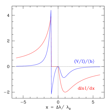
Figure 3: Using the expression from Gayley & Ignace (2012) for a recombination wind emission line threaded by a split monopole magnetic field, $d\ln I/dx$ (red line) and $(V/I)/\left<b\right>$ (blue line) are plotted against the normalized wavelength $x$. The case shown is for an optically thick line with $p=6$.

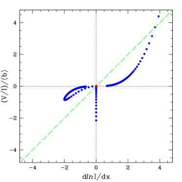
Figure 4: Following Fig. 3, we present a plot of $(V/I)/\left<b\right>$ against $d\ln I/dx$ (blue points). The upper right quadrant is for points in the line profile with $x<-1$. The vertical distribution of points located at $d\ln I/dx$ corresponds to the flat-top portion of the line shape, for $-1<x<0$. The points in the lower left quadrant are for redshifted wavelengths in the line, with $x>0$. The dashed green line is the expected relation for a static atmosphere.

Equation (2) is usually applied to stars with weak winds and no rapid rotation. To qualitatively understand the application of this equation to wind lines in the atmospheres of WR stars, we present in Figs. 3 and 4 the schematic quality of equation (2) in winds, following the model presented in Gayley & Ignace (2012). In these figures, $x$ is the line width in units of the radial Doppler shift at the wind photosphere. $p$ sets the power law for the radial falloff of the volume emissivity. We take $p=6$ to simulate a majority-ion density-squared emissivity in the acceleration zone of a wind with $v\varpropto r$. The $\left<b\right>$ parameter gives the line-of-sight field averaged over the region in the wind that contributes to the profile at $x=1$ in the uniformly expanding wind model with a split monopole field. As this is the region where much of the $V$ signal originates, it provides a reasonable meaning for the average detected field. The unit of $\left<b\right>$ is the field necessary to produce a Zeeman shift equal to the Doppler shift of the radial velocity at the wind photosphere (i.e., the Doppler shift corresponding to $x=1$).

From Fig. 3, we can see that the detailed shape of $V/I$ is not closely proportional to $dlnI/d\lambda$, owing to spatial variations in $\left<B_{\rm z}\right>$ in the detailed model used for those plots, but the overall magnitude of the nonzero $V/I$ is similar, especially for larger $V/I$ that would rise more significantly above the noise. Moreover, there is no reason to expect any correlation whenever the $V/I$ is purely noise. Still, one must accept significant systematic uncertainties in the quantitative meaning of an average longitudial magnetic field in the absence of a specific magnetic field model, so the results quoted are not intended to be directly compared to mean-field upper limits acquired via other means, at a level better than roughly a factor of 2. For this reason, the conclusion by de la Chevrotiére et al. (2013) that the mean longitudinal magnetic field is below about 100 G is not necessarily in conflict with our results, as we see evidence of magnetic fields at the same level as their upper bound (see discussion in Sect. 3).

Linear polarization observations in service mode were obtained for eight angles of the retarder waveplate: $0.0^{\circ}$, $22.5^{\circ}$, $45.0^{\circ}$, $67.5^{\circ}$, $90.0^{\circ}$, $112.5^{\circ}$, $135.0^{\circ}$, $157.5^{\circ}$. During the visitor run in 2010, only the first four positions of the half-wave plate were used.

A net linear polarization from Thomson scattering and line scattering is produced when spherical symmetry is broken. Existing observations revealed that the linear polarization is quite moderate, but, of course, nothing is known about linear polarization for most of the targets in our sample. We note that the linear polarization is of immediate scientific interest itself, as the data can be interpreted not only with respect to deviations from spherical symmetry, but – if variable – also with respect to the temporal evolution of wind structures.

The data reduction for observations of linear polarization was done with the ESO pipeline (v4.9.18) recipes (fors_pmos_calib, fors_pmos_science). For all targets, we calculated the Stokes parameters $P_{Q}=Q/I$ and $P_{U}=U/I$ as defined in Shurcliff (1962).

To calculate the $P_{Q}$ and $P_{U}$ parameters, we used the equations described in the FORS 1/2 User Manual and on the ESO FORS 2 web page (http://www.eso.org/sci/facilities/paranal/instruments/fors/inst/pola.html):

$$\textstyle P_{Q} \textstyle= \textstyle\frac{1}{2}\left\{\left(\frac{f^{o}-f^{e}}{f^{o}+f^{e}}\right)_{\alpha=0^{\circ}}-\left(\frac{f^{o}-f^{e}}{f^{o}+f^{e}}\right)_{\alpha=45^{\circ}}\right\}$$

$$\textstyle+ \textstyle\frac{1}{2}\left\{\left(\frac{f^{o}-f^{e}}{f^{o}+f^{e}}\right)_{\alpha=90^{\circ}}-\left(\frac{f^{o}-f^{e}}{f^{o}+f^{e}}\right)_{\alpha=135^{\circ}}\right\}$$

$$\textstyle P_{U} \textstyle= \textstyle\frac{1}{2}\left\{\left(\frac{f^{o}-f^{e}}{f^{o}+f^{e}}\right)_{\alpha=22.5^{\circ}}-\left(\frac{f^{o}-f^{e}}{f^{o}+f^{e}}\right)_{\alpha=67.5^{\circ}}\right\}$$

$$\textstyle+ \textstyle\frac{1}{2}\left\{\left(\frac{f^{o}-f^{e}}{f^{o}+f^{e}}\right)_{\alpha=112.5^{\circ}}-\left(\frac{f^{o}-f^{e}}{f^{o}+f^{e}}\right)_{\alpha=157.5^{\circ}}\right\}$$

The reduction procedure consists of bias subtraction, flat fielding, extraction, and wavelength calibration of the spectra. The total linear polarization is determined as $P_{L}=\sqrt{P_{Q}^{2}+P_{U}^{2}}$ and the polarization position angle as $\theta_{P}=\frac{1}{2}$ arctan$\left(P_{U}/P_{Q}\right)$. The associated errors for the determination of $P_{Q}$, $P_{U}$, $P_{L}$ and $\theta_{P}$ are estimated from error propagation, based on pure photon noise in the raw data. They are usually of the order of 0.02–0.09% for $P_{Q}$, $P_{U}$ and $P_{L}$, and of about 0.4–1.3^∘ for the determination of $\theta_{P}$.

Since FORS 2 is mounted in the UT 1 Cassegrain focus, its spectropolarimetric calibration is relatively stable. Instrumental polarization measured using unpolarized standard stars is rather low, less than 0.2%. Our observations of the spectropolarimetric standard NGC 2024-1 revealed the values $P_{L}=9.58\pm 0.20$% and $\theta_{P}=136.61\pm 0.42^{\circ}$, which are in very good agreement with the previous measurements $P_{L}=9.65\pm 0.12$% and $\theta_{P}=136.82\pm 0.34^{\circ}$ by Ignace et al. (2009).

3 Results of the magnetic field measurements

Table 3: Longitudinal magnetic field measurements for the entire spectra ($\left<B_{\rm z}\right>_{\rm all}$) and excluding the He ii $\lambda$4686 line ($\left<B_{\rm z}\right>_{-4686}$) for the WR stars observed in 2010. $\left<N_{\rm z}\right>$ values are calculated using the null spectra. All quoted errors are 1$\sigma$ uncertainties.

Object	MJD	SNRcont	$\left<B_{\rm z}\right>_{\textrm{all}}$		$\left<B_{\rm z}\right>_{-4686}$		$\left<N_{\rm z}\right>$
			[G]		[G]		[G]
BAT99 7	55554.1024	1318	37$\pm$	92	327$\pm$	141	66$\pm$	78
BAT99 7	55555.0710	1131	$-$64$\pm$	79	24$\pm$	124	142$\pm$	65
WR 6	55555.1577	1353	131$\pm$	68	258$\pm$	78	11$\pm$	50
WR 7	55554.2477	1028	$-$65$\pm$	46	$-$60$\pm$	49	$-$1$\pm$	46
WR 7	55555.2047	1302	$-$49$\pm$	39	15$\pm$	42	10$\pm$	37
WR 18	55555.2900	1385	$-$86$\pm$	42	$-$76$\pm$	43	$-$19$\pm$	47
WR 23	55554.3245	1600	$-$35$\pm$	34	$-$120$\pm$	48	2$\pm$	28
WR 23	55555.3440	994	$-$87$\pm$	40	$-$80$\pm$	81	65$\pm$	44

The results of our magnetic field measurements using FORS 2 polarimetric spectra obtained in 2010, both for the entire spectrum and for the measurements carried out excluding the strongest emission line belonging to He ii $\lambda$4686 are presented in Table LABEL:tab:bfield_2010_1, where we also collect information on the modified Julian date, the SNR, and the measurements obtained using the null spectra.

Trying to explain the huge rotational velocity of about 160 km s^-1 at the stellar surface of BAT99 7, Shenar et al. (2014) suggested the existence of a very strong photospheric magnetic field of up to 32 kG. The magnetic field of this star was measured on two consecutive nights in 2010, but no detection at a significance of 3$\sigma$ was achieved in either measurement. The magnetic field, if present, would likely be variable. The highest value for the longitudinal magnetic field, $\left<B_{\rm z}\right>_{-4686}=327\pm 141$ G at a significance level of 2.3$\sigma$, was measured on the first night. On the second night, our measurements result in the non-detection $\left<B_{\rm z}\right>_{-4686}=24\pm 124$ G. Certainly, future monitoring of the magnetic field in this star will be worthwhile, to see if there is a field present that is undergoing modulation from rapid rotation, or if the observation is simply random noise.

For WR 23, we measure on the first night $\left<B_{\rm z}\right>_{-4686}=-120\pm 48$ G at a significance level of 2.5$\sigma$ and on the second night $\left<B_{\rm z}\right>_{-4686}=-80\pm 81$ G. For the stars WR 18 and WR 7, magnetic fields are measured at a significance level of about 2$\sigma$ and below.

Among the stars in our sample, only the star WR 6 was reported to show the existence of structures called CIRs, which are believed to be created by density contrasts owing to velocity shear between fast and slow wind streaklines bent by rotation (e.g. Cranmer & Owocki 1996). In some studies also magnetic spots have been invoked as the likely cause of CIRs in hot-star winds. However, previous attempts detected no such fields above several 100 G (e.g., Kholtygin et al. 2011; de la Chevrotiére et al. 2013).

The magnetic field with the highest significance level in our study, with $\left<B_{\rm z}\right>_{-4686}=258\pm 78$ G, was detected in WR 6 during our visitor run in 2010. A first direct search for a magnetic field via the circular polarization of Zeeman splitting in this star was recently carried out by de la Chevrotiére et al. (2013) using the ESPaDOnS spectropolarimeter at the Canada-France-Hawaii Telescope. No magnetic field was unambiguously detected by this team. Assuming that the star is intrinsically magnetic and can be described by a split monopole configuration, the authors found an upper limit on the order of 100 G for the strength of its magnetic field in the line-forming regions of the stellar wind.

Table 4: Longitudinal magnetic field measurements for the entire spectra ($\left<B_{\rm z}\right>_{\textrm{all}}$) and excluding the He ii $\lambda$4686 line ($\left<B_{\rm z}\right>_{-4686}$) for the star WR 6 observed in 2011–2012. $\left<N_{\rm z}\right>$ values are calculated using the null spectra. All quoted errors are 1$\sigma$ uncertainties. The observation on the night of 2011 October 11 had very low SNR and could not be used for the measurement of the magnetic field.

MJD	rotation	rotation	$\left<B_{\rm z}\right>_{\textrm{all}}$		$\left<B_{\rm z}\right>_{-4686}$		$\left<N_{\rm z}\right>$
	phase	cycle	[G]		[G]		[G]
55555.1577	0.560	$-$77	131$\pm$	68	258$\pm$	78	11$\pm$	50
55845.2716	0.596	0	70$\pm$	56	86$\pm$	62	$-$20$\pm$	64
55880.1638	0.861	9	$-$12$\pm$	54	$-$52$\pm$	62	$-$13$\pm$	51
55903.3172	0.009	15	$-$100$\pm$	52	$-$126$\pm$	65	$-$2$\pm$	83
55906.1257	0.754	16	30$\pm$	52	19$\pm$	61	50$\pm$	58
55909.2102	0.573	16	35$\pm$	59	73$\pm$	70	$-$20$\pm$	56
55928.0760	0.583	21	64$\pm$	76	62$\pm$	77	38$\pm$	75
55929.0803	0.849	22	37$\pm$	68	$-$16$\pm$	73	28$\pm$	61
55932.0686	0.643	23	171$\pm$	56	111$\pm$	61	$-$9$\pm$	63
55933.0511	0.904	23	4$\pm$	59	9$\pm$	68	17$\pm$	66
55934.0611	0.172	23	62$\pm$	43	61$\pm$	44	41$\pm$	63
55935.2491	0.487	23	128$\pm$	106	144$\pm$	90	13$\pm$	44

The results of all magnetic field measurements of WR 6 using FORS 2 polarimetric spectra obtained in visitor and service mode, both for the entire spectrum and for the measurements carried out excluding the very strong emission line belonging to He ii $\lambda$4686 are presented in Table LABEL:tab:wr6, where we also give information on the modified Julian date, the rotation phase, and the measurements obtained using null spectra. The phase of each observation was obtained from the mid-times of exposure and the ephemeris given by Lamontagne et al. (1986), based on long-term photometric monitoring ($HJD=2446153.61+3.766E$). We note that the zero point of the phase in our measurements is arbitrary since about 25 years have passed between Lamontagne et al.’s latest data and those presented here for WR 6.

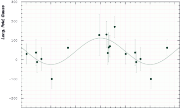
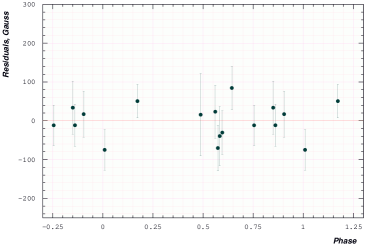
Figure 5: Phase diagram and its best sinusoidal fit for the mean longitudinal magnetic field measurements of WR 6 using the entire spectrum. The residuals (observed – calculated) are shown in the lower panel. The deviations are mostly of the same order as the error bars, and no systematic trends are obvious, which justifies a single sinusoid as a fit function. The sinusoid can be described by an offset of $\overline{\left<B_{\rm z}\right>}=44\pm 15$ G and an amplitude of $A_{\left<B_{\rm az}\right>}=69\pm 21$ G.

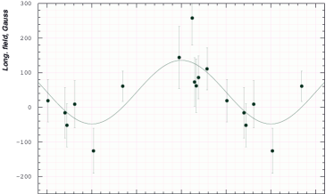
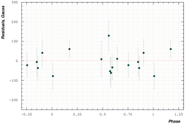
Figure 6: Phase diagram and its best sinusoidal fit for the mean longitudinal magnetic field measurements of WR 6 excluding the He ii $\lambda$4686 line. The residuals (observed – calculated) are shown in the lower panel. The deviations are mostly of the same order as the error bars, and no systematic trends are obvious, which justifies a single sinusoid as a fit function. The sinusoid can be described by an offset of $\overline{\left<B_{\rm z}\right>}=44\pm 17$ G and an amplitude of $A_{\left<B_{\rm az}\right>}=92\pm 24$ G.

Figure 7: Mean longitudinal magnetic field measurements using the null spectra. The overplotted sine curve corresponds to the sinusoidal fit presented in Fig. 5.

The measurements phased with this rotation period using the entire spectrum including all available lines and excluding the He ii $\lambda$4686 line, and the best sinusoidal fits calculated for these measurements, taking into account the already known rotation period $P_{\rm rot}=3.766$ d, are presented in Figs. 5 and 6, respectively. In Fig. 7, we present the mean longitudinal magnetic field measurements using the null spectra. As is shown in this figure, no similar variability of the measured field values using the null spectra is detected over the rotation period. The distribution of the measured values appears random and does not show any trend with the rotation phase.

The field is reversing with the negative and positive field extrema appearing at the rotation phases around 0 and 0.5, respectively. Only two measurements, namely those obtained at the rotation phases of 0.560 and 0.643, reveal statistically significant values of the longitudinal magnetic field at a significance level of 3.3$\sigma$ ($\left<B_{\rm z}\right>_{-4686}=258\pm 78$ G) and 3.1$\sigma$ ($\left<B_{\rm z}\right>_{all}=171\pm 56$ G). A few more measurements show a significance level of about 2$\sigma$. The presence of measurements at lower significance levels in some rotation phases is expected due to the sinusoidal character of the field behaviour with reversing polarities.

From the sinusoidal fits to our data, we obtain for the measurements using the entire spectrum a mean value for the variable longitudinal magnetic field $\overline{\left<B_{\rm z}\right>}=44\pm 15$ G and an amplitude of the field variation $A_{\left<B_{\rm az}\right>}=69\pm 21$ G. Using the entire spectrum without the He ii $\lambda$4686 line, we obtain $\overline{\left<B_{\rm z}\right>}=44\pm 17$ G and $A_{\left<B_{\rm az}\right>}=92\pm 24$ G. For the best fitting models superimposed on the data presented in Figs. 5 and 6, we calculate a reduced $\chi^{2}$ of 0.83 and 0.84, respectively. In contrast, the reduced $\chi^{2}$ values calculated assuming a model in which the longitudinal magnetic field is constant and equal to 0, is 1.56 for the measurements including the He ii 4686 line and 1.92 for the measurements excluding the He ii 4686 line. Noteworthy, we obtain $\chi^{2}=0.44$ for the zero-field model, if we use the $\left<N_{\rm z}\right>$ values obtained using the null spectra.

From the observed sinusoidal modulation, we learn that the magnetic field structure shows two poles and a symmetry axis, tilted with respect to the rotation axis. The simplest model for this magnetic field geometry is based on the assumption that the studied stars are oblique dipole rotators, i.e., their magnetic field can be approximated by a dipole with the magnetic axis inclined to the rotation axis. Of course the strong wind would be expected to extensively modify any simple field geometry, but the precision of the data is insufficient to explore the field in detail.

The angle of obliquity of the magnetic axis $\beta$ is constrained by

$$r=\frac{\left<B_{\rm z}\right>^{\rm min}}{\left<B_{\rm z}\right>^{\rm max}}=\frac{\cos\beta\cos i-\sin\beta\sin i}{\cos\beta\cos i+\sin\beta\sin i},$$ (3)

so that the obliquity angle $\beta$ is given by

$$\beta=\arctan\left[\left(\frac{1-r}{1+r}\right)\cot i\right].$$ (4)

However, because of the dense winds in WR stars, for most of them measuring the projected rotation velocity $v\,\sin\,i$ is not possible, i.e. the rotation axis inclination $i$ remains undefined. Using an estimate of the stellar radius $R=2.65\,R_{\odot}$ for WR 6 (Hamann et al. 2006) and the rotation period $P_{\rm rot}=3.766$ d, we obtain $v_{\rm eq}=35.6$ km s^-1. Since the limb-darkening is also unknown for WR stars, we can only assume that $B_{\rm d}\geq 3\,\left<B_{\rm z}\right>_{\rm max}$ resulting in a minimum dipole strength of $\sim$300–400 G. We note that earlier marginal detections in a few WR stars were determined in the framework of a split monopole magnetic field chosen because of its generic character in a dense, radial stellar wind (Gayley & Ignace 2010). On the other hand, de la Chevrotiére et al. (2014) suggest in their work that the comparison between theoretical predictions and observations should be considered with care.

Based on the presented measurements, we suggest a lower limit for the magnetic field in the line-forming regions of the stellar wind $B_{\rm wind}\sim 300$ G. Since different emission lines form at different distances from the stellar surface and cover different zones of the wind, they sample different field strengths. Knowing roughly the width of the lines, combined with the wind velocity-law index $\beta$, it is possible to approximate the surface field strength, assuming $1/r^{2}$ scaling, where $r=r(v)$. Following the considerations on magnetic and line-emission zone parameters in WR 6 by de la Chevrotiére et al. (2013), we estimate that the surface value of the magnetic field is on the order of a few kiloGauss.

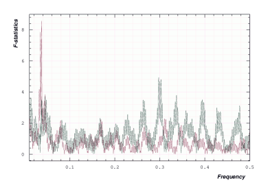
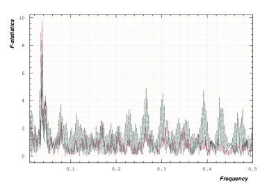
Figure 8: Frequency periodograms (in d^-1) for longitudinal magnetic field measurements using the entire spectrum (upper panel) and for the measurements carried out excluding the He ii $\lambda$4486 line (lower panel). The window function is indicated by the red color.

Interestingly, in spite of the rather low number of magnetic field measurements, the presence of rotation-modulated magnetic variability is also indicated in our frequency periodograms presented in Fig. 8. The periodogram shown in the upper panel was obtained for the measurements using the entire spectrum, while that in the lower panel was obtained for the measurements carried out excluding the He ii $\lambda$4486 line. A frequency analysis was performed using a non-linear least squares fit to the multiple harmonics utilizing the Levenberg-Marquardt method (Press et al. 1992) with the optional possibility of prewhitening the trial harmonics. To detect the most probable period, we calculated the frequency spectrum and for each trial frequency we performed a statistical F-test of the null hypothesis for the absence of periodicity (Seber 1977). The resulting F-statistics can be thought of as the total sum including covariances of the ratio of harmonic amplitudes to their standard deviations, i.e. an SNR. The highest peak in the periodogram obtained for the measurements using the entire spectrum is detected at the frequency 0.30 1/d corresponding to a period of 3.33 d, while the highest peak at the frequency 0.265 1/d corresponding to a period of 3.77 d is identified in the periodogram obtained for the measurements carried out excluding the He ii $\lambda$4486 line.

Figure 9: The variability of the He ii $\lambda$5412 line profile over the rotation cycle. Phased Stokes $I$ profiles are presented with the continuum level set to the rotational phase. For better visibility, all profiles have been scaled by a factor of 0.2.

In the course of our study, we noted that variations detected in emission line profiles probably correlate with the variation of the magnetic field. As an example, we present in Fig. 9 the variability of the shape of the He ii $\lambda$5412 line profile, which shows some kind of double-peak structure in the phases close to the magnetic field extrema, i.e. close to the rotation phases 0 and 0.5. Although our data are rather sparse, it is possible that wind structure variations related to the presence of a magnetic field may lead to the observed changes in the shape of the spectral lines. However, the line profile recorded in 2010 at the phase 0.560 (i.e. 77 rotation cycles before the start of our service observations), which is close to the time of the maximum of the longitudinal magnetic field, does not show this structure. Such instable behaviour of the line profiles in the spectra separated in time by several months or years was previously reported in the study of Flores et al. (2011). Extensive sets of optical spectroscopic observations spread over years have been obtained in the past by several groups, mainly aimed at studies of the relationship between the level of continuum flux emerging from the inner stellar wind and the spectroscopic changes. Despite the epoch dependency of the variations, Morel et al. (1998) found a persistent correlation between changes in the wind line profiles and in the continuum emission forming at the pseudo-photosphere in the wind.

4 Measurement error validation with simulated data

An independent estimate of the error margin of our magnetic field measurements using circular polarization measurements of WR 6 can be obtained from the following test based on simulated data. With the Potsdam Wolf-Rayet (PoWR) model atmosphere code (Gräfener et al. 2002; Hamann & Gräfener 2003), we calculated a synthetic spectrum that is similar to the observed spectrum of this star, presented in Fig. 15 in the work of Hamann et al. (2006).

The advantage of using synthetic models is that they are created without noise and therefore one can add a predetermined amount of noise according to the goodness of the data. At first, we take a normalized model spectrum and reduce the resolution to the FORS 2 standard 2.4 Å FWHM and also bin the pixel size according to the dispersion of 0.75 Å. Then, we add Gaussian distributed noise with a specified SNR. We selected a SNR similar to the observation in the night of 2010 December 24. This procedure is done twice so that one model spectrum with noise can be taken as right circular polarized and the other as left circular polarized. Then the data are analyzed for their Zeeman shift in the same way as the real observations.

This has been done with a SNR of 970 and repeated for $n=10\,000$ times in order to get a normal distributed value of the null field from which it is possible to calculate the standard deviation. This gives an estimate of the expected error for the measurement of the longitudinal magnetic field. The distribution of the measured $\left<B_{\rm z}\right>$ values is plotted as a histogram in Fig. 10. They scatter around zero with a mean deviation of 28 G.

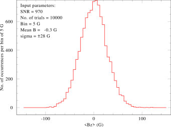
Figure 10: Distribution of $10\,000$ $\left<B_{\rm z}\right>$ measurements on simulated data for WR 6 with input field $\left<B_{\rm z}\right>=0$ and artificial noise corresponding to a SNR of 970 per pixel in each channel. The result shows a 1$\sigma$ error of 28 G.

Summarizing, this test was based on the following assumptions: (1) the line spectrum is similar to our simulated, normalized spectrum for WR 6; (2) the observed spectra have a S/N of 970 per pixel in the ordinary as well as in the extra-ordinary channel; (3) statistical noise is the only source of errors; (4) all lines experience the same Zeeman splitting. Under these assumptions, the value obtained for $\left<B_{\rm z}\right>$ with FORS2 via our method of analysis has a theoretical 1$\sigma$ error of $\sim 28$ G. Note that this error is independent of the magnetic field strength assumed in modeling the simulated Stokes $V$ spectrum (here $\left<B_{\rm z}\right>=0$).

5 Linear polarization

5.1 Linear polarizations of BAT99 7, WR 7, WR 18, and WR 23

Apart from the stars WR 6 and WR 18, no linear polarization observations are reported in the literature for BAT99 7, WR 7, and WR 23. For WR 18, we found in the article of Schulte-Ladbeck (1994) a note that the linear polarization spectrum of this star is featureless. Previous studies of linear polarization of WR 6 indicated the presence of a “line effect”, whereby the polarization across strong lines is generally smaller than in neighboring regions of the continuum (e.g., McLean et al. 1979; Schulte-Ladbeck et al. 1990, 1991; Harries et al. 1999).

Table 5: Continuum linear polarization measurements.

Object	MJD	$Q$		$U$		$P$		$\theta$		Phase
		%		%		[%]		[∘]
BAT99 7	55554.1999	0.52$\pm$	0.04	0.78$\pm$	0.04	0.94$\pm$	0.04	28.16$\pm$	1.22
BAT99 7	55555.1293	0.49$\pm$	0.06	0.75$\pm$	0.06	0.90$\pm$	0.06	28.42$\pm$	1.92
WR 7	55554.2874	1.23$\pm$	0.03	$-$1.76$\pm$	0.03	2.15$\pm$	0.03	$-$27.53$\pm$	0.40
WR 7	55555.2473	1.27$\pm$	0.04	$-$1.74$\pm$	0.04	2.15$\pm$	0.04	$-$26.93$\pm$	0.53
WR 18	55555.3267	$-$0.20$\pm$	0.03	$-$1.91$\pm$	0.03	1.92$\pm$	0.03	$-$47.99$\pm$	0.45
WR 23	55554.3465	$-$2.66$\pm$	0.04	$-$2.99$\pm$	0.04	4.00$\pm$	0.04	$-$65.83$\pm$	0.29
WR 23	55555.3596	$-$2.66$\pm$	0.05	$-$3.01$\pm$	0.05	4.02$\pm$	0.05	$-$65.73$\pm$	0.36
WR 6	55555.1672	0.61$\pm$	0.06	0.02$\pm$	0.06	0.61$\pm$	0.06	0.94$\pm$	2.82	0.563
WR 6	55845.2830	0.22$\pm$	0.05	$-$0.18$\pm$	0.05	0.28$\pm$	0.05	$-$19.64$\pm$	5.04	0.599
WR 6	55846.2701	$-$0.39$\pm$	0.09	$-$0.31$\pm$	0.09	0.50$\pm$	0.09	$-$ 70.76$\pm$	5.18	0.861
WR 6	55880.1753	$-$0.41$\pm$	0.08	$-$0.25$\pm$	0.08	0.48$\pm$	0.08	$-$ 74.31$\pm$	4.77	0.864
WR 6	55903.3289	$-$0.28$\pm$	0.08	0.15$\pm$	0.08	0.32$\pm$	0.08	75.91$\pm$	7.22	0.012
WR 6	55906.1369	0.05$\pm$	0.07	$-$0.38$\pm$	0.07	0.38$\pm$	0.07	$-$41.25$\pm$	5.23	0.758
WR 6	55909.2286	0.32$\pm$	0.07	0.02$\pm$	0.07	0.32$\pm$	0.07	1.79$\pm$	6.25	0.578
WR 6	55928.0893	0.35$\pm$	0.05	$-$0.15$\pm$	0.05	0.38$\pm$	0.05	$-$11.60$\pm$	3.76	0.587
WR 6	55929.1006	$-$0.40$\pm$	0.09	0.32$\pm$	0.09	0.51$\pm$	0.09	70.67$\pm$	5.03	0.855
WR 6	55932.0836	0.27$\pm$	0.05	$-$0.14$\pm$	0.05	0.30$\pm$	0.05	$-$13.70$\pm$	4.71	0.647
WR 6	55933.0627	0.04$\pm$	0.05	0.48$\pm$	0.05	0.48$\pm$	0.05	42.62$\pm$	2.94	0.907
WR 6	55934.07260	0.25$\pm$	0.06	0.03$\pm$	0.06	0.25$\pm$	0.06	3.42$\pm$	6.83	0.175
WR 6	55935.2602	0.28$\pm$	0.07	0.15$\pm$	0.07	0.32$\pm$	0.07	14.09$\pm$	6.31	0.491

In the upper part of Table LABEL:tab:linpol, we present the results of the measurements of linear polarization in the wavelength range between 4000 and 6100 Å for BAT99 7, WR 7, WR 18, and WR 23. For all these stars, the polarization spectra are featureless, i.e. no evidence of a line effect was found. The WR star BAT99 7 is a WN4b type star in the LMC, characterised by very round line profiles. As mentioned in the Introduction, such line profiles are believed to be explained by very rapid rotation that would lead to a deformation of the star. A large deviation from a spherical shape is expected to produce continuum polarization through scattering effects and only the line emission would be less scattered as it originates farther out in the wind. Unfortunately, no line effect is detectable in our linear polarization measurements.

A few years ago, Chené & St-Louis (2011) undertook a search for spectral variability in a large sample of WR stars, among them the stars WR 7, WR 18, and WR 23. While WR 7 and WR 18 showed no detectable spectral variability, the star WR 23 was classified as a star showing small-scale profile variability.

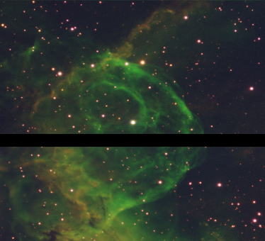
Figure 11: Combined FORS 2 image of the nebula NGC 2359 around the star WR 7. The detector is an E2V mosaic of two 2k$\times$4k CCDs with a field of view of 6.8$\arcmin$$\times$6.8$\arcmin$. The black strip close to the middle of the image is due to a gap between the two chips.

In the observed WR stars, all measured polarization is the sum of interstellar polarization (ISP) and intrinsic polarization. Usually, for stars without a line effect, the polarization properties of nearby field stars are used to estimate the ISP and its position angle. Importantly, narrow-band optical surveys of the environments of WR stars indicate the presence of nebulae around WR 7, WR 18, and WR 23 (Marston 1997). As an example, we present in Fig. 11 an image of the nebula NGC 2359 around the star WR 7, obtained during the target acquisition with FORS 2. This image was obtained by combination of the broad-band $b_{\rm high}$ filter with the narrow-band S ii and H$\alpha$ filters. An interstellar gas shell was also observed in the direction of the WR star WR 6, but presently it is not completely clear whether there is a physical connection between this object and the shell (Nichols & Fesen 1994). Due to the presence of nebulae around our WR targets, we expect that field stars in their vicinity do not probe the same interstellar material and do not display the same ISP. Therefore, no attempt has been made to correct the data for interstellar polarization and the values presented in Table LABEL:tab:linpol cannot be considered as intrinsic to these stars. On the other hand, three WR stars were observed on two different nights, so that our analysis should allow us to detect the presence of variable polarization that is intrinsic to the star. Taking into account the measurement accuracy, no spectropolarimetric variability is detected between the two nights for any star. The star WR 23 shows the largest amount of polarization of about 4%, while the smallest polarization was measured for BAT99 7.

5.2 Interstellar and intrinsic linear polarization of WR 6

Figure 12: Linear polarization spectra of WR 6 not corrected for the interstellar polarization. Each spectrum is shifted in vertical direction by 2% for a better visibility.

Table 6: Spectral regions that were used to measure the mean value of the line and continuum polarization.

Line	line region	continuum region
	[Å]	[Å]
He ii 4201	4196 - 4208	4250 - 4270
He ii 4339	4334 - 4344	4270 - 4290
He ii 4542	4537 - 4547	4430 - 4440
He ii 4859	4855 - 4869	5080 - 5120
He ii 5412	5407 - 5421	5560 - 5730

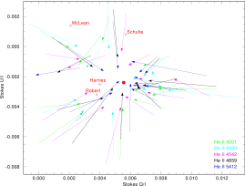
Figure 13: Interstellar polarization of WR 6 determined from the polarization vectors is marked by a filled circle. Previous measurements were carried out by Schulte-Ladbeck et al. (1991), McLean et al. (1979), Robert et al. (1992), and Harries et al. (1999), identified by the individual stars. Vectors are shown for the lines He ii 4201 (light green), He ii 4339 (light blue), He ii 4542 (magenta), He ii 4859 (black), and He ii 5412 (dark blue).

Since all measured polarization is the sum of interstellar polarization and intrinsic polarization (whereby the line polarization is always a fraction of the continuum polarization), to determine the interstellar polarization in WR 6, we followed the procedure described in the work of Harries et al. (1999). In the stellar spectra displaying the line effect, it is possible to obtain a good measure of the interstellar polarization. In order to estimate it, one needs to determine the polarization of the line and the continuum. In Fig. 12, we present as an example linear polarization spectra not corrected for interstellar polarization. The continuum polarization of WR 6 was calculated using the vector sum of the Stokes parameters over the entire spectrum, excluding regions containing obvious emission lines. The respective wavelength regions used are presented in Table 6. This results in a vector pointing from the continuum polarization to the line polarization and finally to the direction of the interstellar polarization (see Fig. 13). Then, we assumed for each observation a line that goes through the line polarization, the continuum polarization and an initial interstellar polarization (ISP). Through a least-squares minimization for each line and a minimization of $\sum\chi^{2}$ via a downhill simplex technique, a best estimate for ($q_{i}$, $u_{i}$) could be determined. We obtained $q_{i}=0.56\pm 0.08$ and $u_{i}=-0.24\pm 0.08$, which gives $P=0.61\pm 0.08\%$ and $\theta=-11.60\pm 3.76^{\circ}$. The interstellar polarization is wavelength dependent and can be modelled by the empirical Serkowski law (Serkowski 1973):

$$P(\lambda)=P_{\textrm{max}}\exp\left[-k\ln^{2}\left(\frac{\lambda_{\textrm{max}}}{\lambda}\right)\right]$$ (5)

where $P_{\textrm{max}}$ is the maximum polarization occurring at a wavelength $\lambda_{\textrm{max}}$ and $k\sim 1.15$ is a shape parameter.

The results of the measurements of linear polarization in the spectra of WR 6 are presented in the lower part of Table LABEL:tab:linpol, together with the corresponding phases. The linear polarization of the star WR 6 was already presented in numerous studies (e.g., Schulte-Ladbeck et al. 1991; McLean et al. 1979; Robert et al. 1992; Harries et al. 1999), and our measurements show close agreement with previous results: we find that the range of the intrinsic continuum polarization is approximately 0.2–0.6%, while the position angle of the polarization is strongly variable. We noticed at the rotation phase 0.855 an apparent emission resulting from the alignment of the continuum to the line polarization and the ISP vector (e.g. Harries et al. 1999). We also noticed that at the rotational phase 0.012 the vector from the continuum to the line polarization significantly differs from all other measurements.

5.3 Modeling a corotating interaction region in WR 6

As mentioned above, WR 6 displays variability that cycles on a period of 3.77 d. This period has generally been associated with rotation, and the star is believed to host a CIR as suggested by UV, optical studies, and X-rays (e.g., St-Louis et al. 1995; Morel et al. 1997; Ignace et al. 2013). The stable period of the star indicates the presence of a clock in the system. However, the variability can exhibit complex behavior, including rapid phase changes (e.g., Antokhin et al. 1994). If the period observed in WR 6 is associated with rotation, then the observed variability is tied to an organized structure threading the wind, such as CIRs. In terms of the period, the linear polarization observations from this study span nearly 100 cycles, and variability in WR 6 is known to exhibit phase drift. However, much of the data were obtained within two contiguous cycles. We have attempted a rough fit to this subset of the linearly polarized data using a CIR model as described in Ignace et al. (2015).

Ignace et al. (2015) presented a kinematic description of a CIR in terms of a spiral arm morphology in shape, and in terms of a density contrast (either enhancement or deficit) relative to the otherwise unperturbed spherical wind. This is clearly a gross simplification as compared to more detailed numerical simulations of CIR phenomena from massive star winds (e.g., Cranmer & Owocki 1996; Dessart 2004). Using this approach, Ignace et al. employ the optically thin scattering results of Brown & McLean (1977) for axisymmetric structures. The spiral morphology is not axisymmetric; however, the structure is conceived in terms of a series of differential pancake-shaped blobs, each one being slightly shifted in azimuth from the preceding, so that each segment of the spiral is axisymmetric. Using an equation of motion for the spiral pattern, and formulating a superposition for the net polarization properties from the ensemble of spiral segment pieces, Ignace et al. were able to evaluate a semi-analytic result for the polarization with rotational phase. Moreover, an approach for combining multiple CIRs originating from arbitrary latitudes was presented.

Here only a heuristic application of the model is applied to the dataset. The model allows for a number of free parameters, but in the application to WR 6, the star and wind parameters are treated as fixed. The wind is optically thick to electron scattering, and the Ignace et al. model applies only for thin scattering. For this situation a core-halo model is adopted, whereby the polarization is evaluated only where the electron optical depth $\tau_{\rm e}<1$, assuming that light from regions with $\tau_{\rm e}>1$ will be completely depolarized.

The free parameters that remain in the model include: viewing inclination $i$ (relative to the spin axis of the star), latitude $\vartheta$ at which a CIR originates, opening angle $\beta$ of the CIR structure, the rotational phase offset $\varphi_{0}$ between the model and the observations, an orientation phase $\psi_{0}$ for how the projected spin axis is projected on the sky relative to the observational system for evaluating Stokes $Q$ and $U$, and finally a density contrast factor $\eta$. Note first that $\eta$ is defined so that $\eta=0$ is a spherical wind. Second, the factors $\beta$ and $\eta$ are somewhat degenerate when the opening angle of the CIR is not overly large: both affect the amplitude of the polarization but not the shape of its variation with rotational phase.

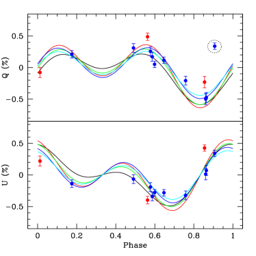
Figure 14: The two panels present linear polarization $Q$ (upper panel) and $U$ (lower panel) in percent plotted against rotational phase. The points present the data while the curves correspond to the models for viewing inclinations of $i=150^{\circ}-165^{\circ}$.

Although the model allows for multiple CIRs, our objective was to determine whether a reasonable match between the data and the model could be achieved with just one CIR structure. The results of our trial-and-error fitting are shown in Fig. 14. The two panels are for $Q$ (upper panel) and $U$ (lower panel) as percent polarization plotted against rotational phase.

Note that formal fits between the data and the model are not made (i.e., there is no $\chi^{2}$ evaluation). Also, the three red points in Fig. 14 were not used in guiding the selection of the model parameters. Of those three points, one is from a much older observation at the phase 0.563, and thus from a much earlier epoch than the blue points. The other two points that were not considered are the point at rotation phase 0.855, where an apparent emission was resulting from the alignment of the continuum to the line polarization and the ISP vector, and the point at rotation phase 0.012, where the vector from the continuum to the line polarization significantly differed from all other measurements (see Sect. 5.2). However, as is shown in Fig. 14, all three points do roughly follow the trend of the model curves.

There is one notable discrepant point in the panel for $Q$, located near phase 0.9 (surrounded by a dotted circle). No model with a single arm can simultaneously account for that point along with the other measurements. The discrepant point may suggest more arms, or that a CIR (or CIRs) is not the only structure existing in the flow. We should expect a stochastic component to the structure. The CIR might be disrupted at times, or perhaps an additional wind structure can sometimes dominate the polarization.

In the selecting the model curves plotted in Figure 14, we first tried a single CIR located in the equatorial plane. Varying the remaining parameters, no satisfactory matches were achievable. Next we varied both the latitude of the CIR and the viewing inclination of the star. A suite of model curves for viewing inclinations of $i=150^{\circ}-165^{\circ}$ are displayed in Fig. 14, which are seen to broadly reproduce the pattern for the data (with the exception of one point in $Q$ near phase of 0.9). Relative to inclinations below $90^{\circ}$, an inclination exceeding $90^{\circ}$ serves to flip the sense of rotation as projected onto the sky. For this range a fairly similar set of model curves resulted for CIRs at latitudes of $40^{\circ}$ and $45^{\circ}$ as well as $135^{\circ}$ and $140^{\circ}$. When $i$ and $\vartheta$ are in opposite hemispheres, the spiral does sweep across the front of the star for the observer’s sightline, but WR 6 is known to show regular DAC behavior (e.g. St-Louis et al. 1995). Figure 14 thus shows the models for $\vartheta=135^{\circ}$ and $140^{\circ}$.

This is the first time that a model for polarization from a CIR has been applied to data. Given that the model adopts a core-halo approach, plus the complexity of the wind structure, the overall ability of the model to match the majority of the data suggests that a CIR is plausibly the source, or a significant contributor, to the variable linear polarimetry of WR 6. It is not our goal to claim a fit of high significance, but simply to test the ability of the model for achieving a rough match to the observed trend with (a) a single CIR and (b) a limited number of free parameters. Given the simplistic nature of the model, it is gratifying to find that a modestly good fit to the majority of the measures can be achieved.

6 Discussion

In this work, we address Wolf-Rayet type stars, where the magnetic fields are especially hard to detect because of the wind-broadening of their spectral lines. Moreover, all photospheric lines are absent and the magnetic field is measured on emission lines formed in the strong wind.

It is the first time that the low dispersion spectrograph FORS 2 in spectropolarimetric mode mounted at one of the biggest telescopes in the world is used for spectropolarimetry of WR stars. WR stars descend from initial masses above 20 $M_{\odot}$ and during their fast evolution, they already lost a significant mass fraction via their powerful stellar winds. Depending on their exact mass, rotation, magnetism and mass-loss, in a few $10^{5}$ yr, these stars will become either neutron stars or black holes (e.g. Heger et al. 2003). A small fraction of the WR star progenitors have strong magnetic fields on the main sequence – the magnetic O-type stars. The observed temporal variations of the longitudinal magnetic fields in these stars are usually compatible with dipole fields inclined to the rotation axis, implying a simple global structure. Obviously, the strength of the average longitudinal magnetic field in WR 6, varying with an amplitude of order only 100 G over the rotation cycle, is significantly lower than the field strength detected in several magnetic O-type stars. This is perhaps not surprising, given the fact that the magnetic field is diagnosed in the line-forming regions, which fall fairly far out in a Wolf-Rayet wind, and not at the stellar surface. On the other hand, a Wolf-Rayet star like WR 6 is significantly contracted relative to its O-star progenitor, so the evolution of the field between these states requires further investigation. It would be worthwhile to obtain in the future more dense rotation phase coverage by spectropolarimetric observations to further strengthen the evidence for the magnetic nature of this star. We should keep in mind that the method we have applied involves substantial systematic uncertainties, so only gives a rough result for the field strength where lines are formed, and that different lines form over different zones of the wind, sampling different field strengths.

Magnetic fields for the other WR stars in our sample present at a significance level of about 2.5$\sigma$ and below. Since up to now no long-time spectropolarimetric monitoring was carried out for them and we cannot neglect the possibility of unfavorable sampling of the magnetic field configuration, the non-detection of the magnetic field does not mean that no magnetic field is present in their atmospheres. Clearly, attaining higher SNR using FORS 2 in the future will help to set more stringent limits to their magnetic field strengths.

For the first time, we present linear polarization measurements for BAT99 7, WR 7, WR 18, and WR 23. We do not find any evidence of a line effect in these stars. Previous linear polarization studies showed that most WR stars exhibit variable continuum polarization. However, no spectropolarimetric variability is detected for BAT99 7, WR 7, and WR 23 over two nights. From the monitoring of the linear polarization of WR 6 over the rotation cycle, we confirm that the detected continuum polarization and the polarization position angle are not constant with time.

References

- Angel & Landstreet (1970) Angel J. R. P., Landstreet J. D., 1970, ApJ, 160, L147
- Appenzeller et al. (1998) Appenzeller I., Fricke W., Fürtig W., et al., 1998, The ESO Messenger, 94, 1
- Antokhin et al. (1994) Antokhin I., Bertrand J-F., Lamontagne R., Moffat A. F., 1994, AJ, 107,2179
- Bagnulo et al. (2012) Bagnulo S., Landstreet J. D., Fossati L., Kochukhov O., 2012, A&A, 538, A129
- Bailey et al. (2015) Bailey J. D., Grunhut J., Landstreet J. D., 2015, A&A, 575, A115
- Brown & McLean (1977) Brown J. C., McLean I. S., 1977, A&A, 57, 141
- Cantiello et al. (2009) Cantiello M., et al., 2009, A&A, 499, 279
- Chené & St-Louis (2011) Chené A.-N., St-Louis N., 2011, ApJ, 736, 140
- Cranmer & Owocki (1996) Cranmer S., Owocki S., 1996, ApJ, 462, 469
- de la Chevrotiére et al. (2013) de la Chevrotiére A., St-Louis N., Moffat A. F. J., MiMeS Collaboration, 2013, ApJ, 764, 171
- de la Chevrotiére et al. (2014) de la Chevrotiére A., St-Louis N., Moffat A. F. J., MiMeS Collaboration, 2014, ApJ, 781, 73
- Dessart (2004) Dessart L., 2004, A&A, 423, 693
- Feldmeier et al. (1997) Feldmeier A., Puls J., Pauldrach A. W. A., 1997, A&A, 322, 878
- Flores et al. (2011) Flores A., Koenigsberger G., Cardona O., de La Cruz L., 2011, RMxAA, 47, 261
- Fossati et al. (2015) Fossati L., et al., 2015, A&A, 582, A45
- Gayley & Ignace (2010) Gayley K. G., Ignace R., 2010, ApJ, 708, 615
- Gayley & Ignace (2012) Gayley K. G., Ignace R., 2012, AIP Conf. Proc., Volume 1429, pp. 259-262
- Gayley & Owocki (1995) Gayley K. G., Owocki, S. P., 1995, ApJ, 565, 545
- Gräfener et al. (2002) Gräfener G., Koesterke L., Hamann W.-R., 2002, A&A, 387, 244
- Hainich et al. (2014) Hainich R., et al., 2014, A&A, 565, A27
- Hamann & Gräfener (2003) Hamann W.-R., Gräfener G., 2003, A&A, 410, 993
- Hamann et al. (2006) Hamann W.-R., Gräfener G., Liermann A., 2006, A&A, 457, 1015
- Harries et al. (1999) Harries T. J., Howarth I. D., Schulte-Ladbeck R. E., Hillier D. J., 1999, MNRAS, 302, 499
- Heger et al. (2003) Heger A., Fryer C. L., Woosley S. E., Langer N., Hartmann D. H., 2003, ApJ, 591, 288
- Hubrig et al. (2004a) Hubrig S., Kurtz, D. W., Bagnulo S., Szeifert T., Schöller M., Mathys G., Dziembowski W. A., 2004a, A&A, 415, 661
- Hubrig et al. (2004b) Hubrig S., Szeifert T., Schöller M., Mathys G., Kurtz D. W., 2004b, A&A, 415, 685
- Hubrig et al. (2008) Hubrig S., Schöller M., Schnerr R. S., González J. F., Ignace R., Henrichs H. F., 2008, A&A, 490, 793
- Hubrig et al. (2011) Hubrig S., et al., 2011, A&A, 528, A151
- Hubrig et al. (2013) Hubrig S., et al., 2013, A&A, 551, A33
- Hubrig et al. (2014) Hubrig S., Schöller M., Kholtygin A. F., 2014, MNRAS, 440, 1779
- Hubrig et al. (2015) Hubrig S., et al., 2015, MNRAS, 447, 1885
- Ignace et al. (2009) Ignace R., Hubrig S., Schöller M., 2009, AJ, 137, 3339
- Ignace et al. (2013) Ignace R., Gayley K. G., Hamann W.-R., Huenemoerder D. P., Oskinova L. M., Pollock A. M. T., McFall M., 2013, ApJ, 775, 29
- Ignace et al. (2015) Ignace R., St-Louis N., Proulx-Giraldeau F., 2015, A&A, 575, 129
- Kholtygin et al. (2011) Kholtygin A. F., Fabrika S. N., Rusomarov N., Hamann W.-R., Kudryavtsev D. O., Oskinova L. M., Chountonov, G. A., 2011, AN, 332, 1008
- Lamontagne et al. (1986) Lamontagne R., Moffat A. F. J., Lamarre A., 1986, AJ, 91, 925
- Maeder & Meynet (2005) Maeder A., Meynet G., 2005, A&A, 440, 1041
- Marston (1997) Marston A. P., 1997, ApJ, 475, 188
- McLean et al. (1979) McLean I. S., Coyne G. V., Frecker S. J. J. E., Serkowski K., 1979, ApJ, 231, L141
- Michaux et al. (2014) Michaux Y. J. L., Moffat A. F. J., Chené A.-N., St-Louis, N., 2014, MNRAS, 440, 2
- Morel et al. (1997) Morel T., St-Louis N., Marchenko S. V., 1997, ApJ, 482, 470
- Morel et al. (1998) Morel T., St-Louis N., Moffat A. F. J., 1998, ApJ, 498, 413
- Mullan (1984) Mullan D. J., 1984, ApJ, 283, 303
- Mullan & MacDonald (2005) Mullan D. J., MacDonald J., 2005, MNRAS, 356, 1139
- Nichols & Fesen (1994) Nichols J. S., Fesen R. A., 1994, A&A, 291, 283
- Oskinova et al. (2009) Oskinova L. M., Hamann W.-R., Feldmeier A., Ignace R., Chu Y.-H., 2009, ApJ, 693, L44
- Press et al. (1992) Press W. H., Teukolsky S. A., Vetterling W. T., Flannery B. P., 1992, Numerical Recipes, 2nd edn. (Cambridge: Cambridge University Press)
- Ramiaramanantsoa et al. (2014) Ramiaramanantsoa T., et al., 2014, MNRAS, 441, 910
- Robert et al. (1992) Robert C., et al., 1992, ApJ, 397, 277
- Sander et al. (2012) Sander A., Hamann W.-R., Todt H., 2012, A&A, 540, A144
- Schulte-Ladbeck (1994) Schulte-Ladbeck R. E., 1994, Ap&SS, 221, 347
- Schulte-Ladbeck et al. (1990) Schulte-Ladbeck R. E., Nordsieck K. H., Nook M. A., Magalhaes A. M., Taylor M., Bjorkman K. S., Anderson C. M., 1990, ApJ, 365, L19
- Schulte-Ladbeck et al. (1991) Schulte-Ladbeck R. E., Nordsieck K. H., Taylor M., Nook M. A., Bjorkman K. S., Magalhaes A. M., Anderson C. M., 1991, ApJ, 382, 301
- Seber (1977) Seber G. A. F., 1977, Linear Regression Analysis (New York: Wiley)
- Serkowski (1973) Serkowski K., 1973, Interstellar Polarization, in Interstellar Dust and Related Topics, ed., J. M. Greenberg, H. C. van de Hulst, IAU Symposium, 52, 145
- Shenar et al. (2014) Shenar T., Hamann W.-R., Todt H., 2014, A&A, 562, A118
- Shurcliff (1962) Shurcliff W. A., 1962, Polarized light (Harvard Univ. Press, Cambridge)
- Spruit (2002) Spruit H. C., 2002, A&A, 381, 923
- St-Louis et al. (1995) St-Louis N., Dalton M. J., Marchenko S. V., Moffat A. F. J., Willis A. J., 1995, ApJ, 452, L57
- ud-Doula & Owocki (2002) ud-Doula A., Owocki S. P., 2002, ApJ, 576, 413
- Waldron & Cassinelli (2007) Waldron W. L., Cassinelli J. P., 2007, ApJ, 668, 456
- Waldron & Cassinelli (2009) Waldron W. L., Cassinelli J. P., 2009, ApJ, 692, L76