Implementation of a Direct Coupling Coherent Quantum Observer including Observer Measurements

Abstract

This paper considers the problem of constructing a direct coupling quantum observer for a quantum harmonic oscillator system. The proposed observer is shown to be able to estimate one but not both of the plant variables and produces a measureable output using homodyne detection.

I Introduction

A number of papers have recently considered the problem of constructing a coherent quantum observer for a quantum system; e.g., see [1, 2, 3, 4]. In the coherent quantum observer problem, a quantum plant is coupled to a quantum observer which is also a quantum system. The quantum observer is constructed to be a physically realizable quantum system so that the system variables of the quantum observer converge in some suitable sense to the system variables of the quantum plant. The papers [4, 5, 6, 7] considered the problem of constructing a direct coupling quantum observer for a given closed quantum system. In [4], the proposed observer is shown to be able to estimate some but not all of the plant variables in a time averaged sense. Also, the paper [8] shows that a possible experimental implementation of the augmented quantum plant and quantum observer system considered in [4] may be constructed using a non-degenerate parametric amplifier (NDPA) which is coupled to a beamsplitter by suitable choice of the NDPA and beamsplitter parameters.

One important limitation of the direct coupled quantum observer results given in [4, 5, 6, 7, 8] is that both the quantum plant and the quantum observer are closed quantum systems. This means that it not possible to make an experimental measurement to verify the properties of the quantum observer. In this paper, we address this difficulty by extending the results of [4] to allow for the case in which the quantum observer is an open quantum linear system whose output can be monitored using homodyne detection. In this case, it is shown that similar results can be obtained as in [4] except that now the observer output is subject to a white noise perturbation. However, by suitably designing the observer, it is shown that the level of this noise perturbation can be made arbitrarily small (at the expense of slow observer convergence). Also, the results of [8] are extended to show that a possible experimental implementation of the augmented quantum plant and quantum observer system may be constructed using a non-degenerate parametric amplifier (NDPA) which is coupled to a beamsplitter by suitable choice of the NDPA and beamsplitter parameters. In this case, the NDPA contains an extra field channel as compared to the result in [8] and this extra channel is used for homodyne detection in the observer.

II Direct Coupling Coherent Quantum Observer with Observer Measurement

In this section, we extend the theory of [4] to the case of a direct coupled quantum observer which is also coupled to a field to enable measurements to be made on the observer. In our proposed direct coupled coherent quantum observer, the quantum plant is a single quantum harmonic oscillator which is a linear quantum system (e.g., see [9, 10, 11, 12, 13]) described by the non-commutative differential equation

$$\dot{x}_{p}(t) = 0;\quad x_{p}(0)=x_{0p};$$

$$z_{p}(t) = C_{p}x_{p}(t)$$ (1)

where $z_{p}(t)$ denotes the system variable to be estimated by the observer and $C_{p}\in\mathbb{R}^{1\times 2}$. This quantum plant corresponds to a plant Hamiltonian $\mathcal{H}_{p}=0$. Here $x_{p}=\left[\begin{array}[]{l}q_{p}\\ p_{p}\end{array}\right]$ where $q_{p}$ is the plant position operator and $p_{p}$ is the plant momentum operator. It follows from (1) that the plant system variables $x_{p}(t)$ will remain fixed if the plant is not coupled to the observer.

We now describe the linear quantum system which will correspond to the quantum observer; see also [9, 10, 11, 12, 13]. This system is described by a quantum stochastic differential equation (QSDE) of the form

$$dx_{o} = A_{o}x_{o}dt+B_{o}dw;\quad x_{o}(0)=x_{0o};$$

$$dy_{o} = C_{o}x_{o}dt+dw;$$

$$z_{o}(t) = Ky_{o}$$ (2)

where $dw=\left[\begin{array}[]{l}dQ\\ dP\end{array}\right]$ is a $2\times 1$ vector of quantum noises expressed in quadrature form corresponding to the input field for the observer and $dy_{o}$ is the corresponding output field; e.g., see [9, 11]. The observer output $z_{o}(t)$ will be a real scalar quantity obtained by applying homodyne detection to the observer output field. $A_{o}\in\mathbb{R}^{2\times 2}$, $B_{o}\in\mathbb{R}^{2\times 2}$, $C_{o}\in\mathbb{R}^{2\times 2}$. Also, $x_{o}(t)=\left[\begin{array}[]{l}q_{o}\\ p_{o}\end{array}\right]$ is a vector of self-adjoint system variables corresponding to the observer position and momentum operators; e.g., see [9]. We assume that the plant variables commute with the observer variables. The system dynamics (2) are determined by the observer system Hamiltonian and coupling operators which are operators on the underlying Hilbert space for the observer. For the quantum observer under consideration, this Hamiltonian is a self-adjoint operator given by the quadratic form: $\mathcal{H}_{o}=\frac{1}{2}x_{o}(0)^{T}R_{o}x_{o}(0)$, where $R_{o}$ is a real symmetric matrix. Also, the coupling operator $L$ is defined by a matrix $W_{o}\in\mathbb{R}^{2\times 2}$ so that

$$\left[\begin{array}[]{c}L+L^{*}\\ \frac{L-L^{*}}{i}\end{array}\right]=W_{o}x_{o}.$$ (3)

Then, the corresponding matrices $A_{o}$, $B_{o}$ and $C_{o}$ in (2) are given by

$$A_{o}=2JR_{o}+\frac{1}{2}W_{o}^{T}JW_{o},~{}~{}B_{o}=JW_{o}^{T}J,~{}~{}C_{o}=W_{o}$$ (4)

where

$$J=\left[\begin{array}[]{ll}0&1\\ -1&0\end{array}\right];$$

e.g., see [9, 11]. Furthermore, we will assume that the quantum observer is coupled to the quantum plant as shown in Figure 1.

Figure 1: Plant Observer System.

In addition, we define a coupling Hamiltonian which defines the coupling between the quantum plant and the quantum observer:

$$\mathcal{H}_{c}=x_{p}(0)^{T}R_{c}x_{o}(0).$$

The augmented quantum linear system consisting of the quantum plant and the quantum observer is then a linear quantum system described by the total Hamiltonian

$$\mathcal{H}_{a} = \mathcal{H}_{p}+\mathcal{H}_{c}+\mathcal{H}_{o}$$ (5)

$$= \frac{1}{2}x_{a}(0)^{T}R_{a}x_{a}(0)$$

where

$$x_{a}=\left[\begin{array}[]{l}x_{p}\\ x_{o}\end{array}\right],~{}~{}R_{a}=\left[\begin{array}[]{ll}0&R_{c}\\ R_{c}^{T}&R_{o}\end{array}\right],$$ (6)

and the coupling operator $L$ defined in (3). Extending the approach used in [4], we assume that we can write

$$R_{c}=\alpha\beta^{T},$$ (7)

$R_{o}=\omega_{o}I$, $W_{o}=\sqrt{\kappa}I$ where $\alpha\in\mathbb{R}^{2}$, $\beta\in\mathbb{R}^{2}$, $\omega_{o}>0$ and $\kappa>0$. In addition, we assume

$$\alpha=C_{p}^{T}.$$ (8)

Then, we can write the QSDEs describing the closed loop system as follows:

$$dx_{p} = 2J\alpha\beta^{T}x_{o}dt;$$

$$dx_{o} = 2\omega_{o}Jx_{o}dt+2J\beta\alpha^{T}x_{p}dt+\frac{1}{2}JW_{o}^{T}JW_{o}x_{o}dt$$ (11)

$$+JW_{o}^{T}Jdw$$

$$= \left[\begin{array}[]{ll}-\frac{\kappa}{2}&2\omega_{o}\\ -2\omega_{o}&-\frac{\kappa}{2}\end{array}\right]x_{o}dt+2J\beta\alpha^{T}x_{p}dt-\sqrt{\kappa}dw;$$

$$dy_{o} = W_{o}x_{o}dt+dw$$ (12)

$$= \sqrt{\kappa}x_{o}dt+dw;$$

e.g., see [9, 11]. Now it follow from (1) and (8) that

$$z_{p}=\alpha^{T}x_{p}.$$

Hence, it follows from the first equation in (II) that

$$dz_{p}=2\alpha^{T}J\alpha\beta^{T}x_{o}dt=0.$$

That is, the quantity $z_{p}$ remains constant even after the quantum plant is coupled to the quantum observer. In addition, we can re-write the remaining equations in (II) as

$$dx_{o} = \left[\begin{array}[]{ll}-\frac{\kappa}{2}&2\omega_{o}\\ -2\omega_{o}&-\frac{\kappa}{2}\end{array}\right]x_{o}dt+2J\beta z_{p}dt-\sqrt{\kappa}dw;$$ (15)

$$dy_{o} = \sqrt{\kappa}x_{o}dt+dw;$$ (16)

To analyse the system (15), we first calculate the steady state value of the quantum expectation of the observer variables as follows:

$$<\bar{x}_{o}> = -2\left[\begin{array}[]{ll}-\frac{\kappa}{2}&2\omega_{o}\\ -2\omega_{o}&-\frac{\kappa}{2}\end{array}\right]^{-1}J\beta z_{p}$$

$$= \frac{4}{\kappa^{2}+16\omega_{o}^{2}}\left[\begin{array}[]{ll}\kappa&4\omega_{o}\\ -4\omega_{o}&\kappa\end{array}\right]J\beta z_{p}.$$

Then, we define the quantity

$$\tilde{x}_{o}=x_{o}-<\bar{x}_{o}>=x_{o}-\frac{4}{\kappa^{2}+16\omega_{o}^{2}}\left[\begin{array}[]{ll}\kappa&4\omega_{o}\\ -4\omega_{o}&\kappa\end{array}\right]J\beta z_{p}.$$

We can now re-write the equations (15) in terms of $\tilde{x}_{0}$ as follows

$$d\tilde{x}_{o} = \left[\begin{array}[]{ll}-\frac{\kappa}{2}&2\omega_{o}\\ -2\omega_{o}&-\frac{\kappa}{2}\end{array}\right]x_{o}dt+2J\beta z_{p}dt-\sqrt{\kappa}dw$$ (21)

$$= \left[\begin{array}[]{ll}-\frac{\kappa}{2}&2\omega_{o}\\ -2\omega_{o}&-\frac{\kappa}{2}\end{array}\right]\tilde{x}_{o}dt$$

$$-2\left[\begin{array}[]{ll}-\frac{\kappa}{2}&2\omega_{o}\\ -2\omega_{o}&-\frac{\kappa}{2}\end{array}\right]\left[\begin{array}[]{ll}-\frac{\kappa}{2}&2\omega_{o}\\ -2\omega_{o}&-\frac{\kappa}{2}\end{array}\right]^{-1}J\beta z_{p}dt$$

$$+2J\beta z_{p}dt-\sqrt{\kappa}dw$$

$$= \left[\begin{array}[]{ll}-\frac{\kappa}{2}&2\omega_{o}\\ -2\omega_{o}&-\frac{\kappa}{2}\end{array}\right]\tilde{x}_{o}dt-\sqrt{\kappa}dw;$$ (32)

$$dy_{o} = \sqrt{\kappa}\tilde{x}_{o}dt-2\sqrt{\kappa}\left[\begin{array}[]{ll}-\frac{\kappa}{2}&2\omega_{o}\\ -2\omega_{o}&-\frac{\kappa}{2}\end{array}\right]^{-1}J\beta z_{p}dt+dw$$ (35)

$$= -2\sqrt{\kappa}\left[\begin{array}[]{ll}-\frac{\kappa}{2}&2\omega_{o}\\ -2\omega_{o}&-\frac{\kappa}{2}\end{array}\right]^{-1}J\beta z_{p}dt+dw^{out}$$ (38)

where

$$dw^{out}=\sqrt{\kappa}\tilde{x}_{o}dt+dw.$$

We now look at the transfer function of the system

$$d\tilde{x}_{o} = \left[\begin{array}[]{ll}-\frac{\kappa}{2}&2\omega_{o}\\ -2\omega_{o}&-\frac{\kappa}{2}\end{array}\right]\tilde{x}_{o}dt-\sqrt{\kappa}dw;$$ (41)

$$dw^{out} = \sqrt{\kappa}\tilde{x}_{o}dt+dw$$ (42)

which is given by

$$G(s)=-\kappa\left[\begin{array}[]{ll}s+\frac{\kappa}{2}&-2\omega_{o}\\ 2\omega_{o}&s+\frac{\kappa}{2}\end{array}\right]^{-1}.$$

It is straightforward to verify that this transfer function is such that

$$G(j\omega)G(j\omega)^{\dagger}=I$$

for all $\omega$. That is $G(s)$ is all pass. Also, the matrix $\left[\begin{array}[]{ll}-\frac{\kappa}{2}&2\omega_{o}\\ -2\omega_{o}&-\frac{\kappa}{2}\end{array}\right]$ is Hurwitz and hence, the system (41) will converge to a steady state in which $dw^{out}$ represents a standard quantum white noise with zero mean and unit intensity. Hence, at steady state, the equation

$$dy_{o}=-2\sqrt{\kappa}\left[\begin{array}[]{ll}-\frac{\kappa}{2}&2\omega_{o}\\ -2\omega_{o}&-\frac{\kappa}{2}\end{array}\right]^{-1}J\beta z_{p}dt+dw^{out}$$ (43)

shows that the output field converges to a constant value plus zero mean white quantum noise with unit intensity.

We now consider the construction of the vector $K$ defining the observer output $z_{o}$. This vector determines the quadrature of the output field which is measured by the homodyne detector. We first re-write equation (43) as

$$dy_{o}=ez_{p}dt+dw^{out}$$

where

$$e=-2\sqrt{\kappa}\left[\begin{array}[]{ll}-\frac{\kappa}{2}&2\omega_{o}\\ -2\omega_{o}&-\frac{\kappa}{2}\end{array}\right]^{-1}J\beta$$ (44)

is a vector in $\mathbb{R}^{2}$. Then

$$dz_{o}=Kez_{p}dt+Kdw^{out}.$$

Hence, we choose $K$ such that

$$Ke=1$$ (45)

and therefore

$$dz_{o}=z_{p}dt+dn$$

where

$$dn=Kdw^{out}$$

will be a white noise process at steady state with intensity $\|K\|^{2}$. Thus, to maximize the signal to noise ratio for our measurement, we wish to choose $K$ to minimize $\|K\|^{2}$ subject to the constraint (45). Note that it follows from (45) and the Cauchy-Schwartz inequality that

$$1\leq\|K\|\|e\|$$

and hence

$$\|K\|\geq\frac{1}{\|e\|}.$$

However, if we choose

$$K=\frac{e^{T}}{\|e\|^{2}}$$ (46)

then (45) is satisfied and $\|K\|=\frac{1}{\|e\|}$. Hence, this value of $K$ must be the optimal $K$.

We now consider the special case of $\omega_{o}=0$. In this case, we obtain

$$e=2\sqrt{\kappa}\left[\begin{array}[]{ll}\frac{2}{\kappa}&0\\ 0&\frac{2}{\kappa}\end{array}\right]J\beta=\frac{4}{\sqrt{\kappa}}J\beta.$$

Hence, as $\kappa\rightarrow 0$, $\|e\|\rightarrow\infty$ and therefore $\|K\|\rightarrow 0$. This means that we can make the noise level on our measurement arbitrarily small by choosing $\kappa>0$ sufficiently small. However, as $\kappa$ gets smaller, the system (41) gets closer to instability and hence, takes longer to converge to steady state.

III A Possible Implementation of the Plant Observer System

In this section, we describe one possible experimental implementation of the plant-observer system given in the previous section. The plant-observer system is a linear quantum system with Hamiltonian

$$\mathcal{H}_{c}+\mathcal{H}_{o}=x_{p}^{T}R_{c}x_{o}+\frac{1}{2}x_{o}^{T}R_{o}x_{o}$$ (47)

and coupling operator defined so that

$$\left[\begin{array}[]{c}L+L^{*}\\ \frac{L-L^{*}}{i}\end{array}\right]=W_{o}x_{o}.$$

Furthermore, we assume that $R_{c}=\alpha\beta^{T}$, $R_{o}=\omega_{o}I$, $W_{o}=\sqrt{\kappa}I$ where $\alpha\in\mathbb{R}^{2}$, $\beta\in\mathbb{R}^{2}$, $\omega_{o}>0$ and $\kappa>0$.

In order to construct a linear quantum system with a Hamiltonian of this form, we consider an NDPA coupled to a beamsplitter as shown schematically in Figure 2; e.g., see [14].

Figure 2: NDPA coupled to a beamsplitter.

A linearized approximation for the NDPA is defined by a quadratic Hamiltonian of the form

$$\mathcal{H}_{1}=\frac{\imath}{2}\left(\epsilon a^{*}b^{*}-\epsilon^{*}ab\right)+\frac{1}{2}\omega_{o}b^{*}b$$

where $a$ is the annihilation operator corresponding to the first mode of the NDPA and $b$ is the annihilation operator corresponding to the second mode of the NDPA. These modes will be assumed to be of the same frequency but with a different polarization with $a$ corresponding to the quantum plant and $b$ corresponding to the quantum observer. Also, $\epsilon$ is a complex parameter defining the level of squeezing in the NDPA and $\omega_{o}$ corresponds to the detuning frequency of the $b$ mode in the NDPA. The $a$ mode in the NDPA is assumed to be tuned. In addition, the NDPA corresponds to a vector of coupling operators $L=\left[\begin{array}[]{l}\sqrt{\kappa_{1}}a\\ \sqrt{\kappa_{2}}b\\ \sqrt{\kappa_{3}}b\end{array}\right]$. Here $\kappa_{1}>0$, $\kappa_{2}>0$, $\kappa_{3}>0$ are scalar parameters determined by the reflectance of the mirrors in the NDPA.

From the above Hamiltonian and coupling operators, we can calculate the following quantum stochastic differential equations (QSDEs) describing the NDPA:

$$\left[\begin{array}[]{l}da\\ db\end{array}\right] = \left[\begin{array}[]{ll}0&\frac{\epsilon}{2}\\ \frac{\epsilon}{2}&0\end{array}\right]\left[\begin{array}[]{l}a^{*}\\ b^{*}\end{array}\right]dt$$ (65)

$$-\left[\begin{array}[]{ll}\frac{\gamma_{1}}{2}&0\\ 0&\frac{\gamma_{2}}{2}+\frac{1}{2}\imath\omega_{o}\end{array}\right]\left[\begin{array}[]{l}a\\ b\end{array}\right]dt$$

$$-\left[\begin{array}[]{lll}\sqrt{\kappa_{1}}&0&0\\ 0&\sqrt{\kappa_{2}}&\sqrt{\kappa_{3}}\end{array}\right]\left[\begin{array}[]{l}dA\\ dB_{1}\\ dB_{2}\end{array}\right];$$

$$\left[\begin{array}[]{l}dA^{out}\\ dB_{1}^{out}\\ dB_{2}^{out}\end{array}\right] = \left[\begin{array}[]{ll}\sqrt{\kappa_{1}}&0\\ 0&\sqrt{\kappa_{2}}\\ 0&\sqrt{\kappa_{3}}\end{array}\right]\left[\begin{array}[]{l}a\\ b\end{array}\right]dt+\left[\begin{array}[]{l}dA\\ dB_{1}\\ dB_{2}\end{array}\right];$$ (77)

where $\gamma_{1}=\kappa_{1}$ and $\gamma_{2}=\kappa_{2}+\kappa_{3}$.

We now consider the equations defining the beamsplitter

$$\left[\begin{array}[]{l}A\\ B_{1}\end{array}\right]=\left[\begin{array}[]{ll}\cos\theta&e^{-\imath\phi}\sin\theta\\ -e^{\imath\phi}\sin\theta&\cos\theta\end{array}\right]\left[\begin{array}[]{l}A^{out}\\ B_{1}^{out}\end{array}\right]$$

where $\theta$ and $\phi$ are angle parameters defining the beamsplitter; e.g., see [15]. This implies

$$\left[\begin{array}[]{l}A^{out}\\ B_{1}^{out}\end{array}\right]=\left[\begin{array}[]{ll}\cos\theta&-e^{-\imath\phi}\sin\theta\\ e^{\imath\phi}\sin\theta&\cos\theta\end{array}\right]\left[\begin{array}[]{l}A\\ B_{1}\end{array}\right].$$

Substituting this into the second equation in (65), we obtain

$$\left[\begin{array}[]{ll}\cos\theta&-e^{-\imath\phi}\sin\theta\\ e^{\imath\phi}\sin\theta&\cos\theta\end{array}\right]\left[\begin{array}[]{l}dA\\ dB_{1}\end{array}\right]$$

$$=\left[\begin{array}[]{ll}\sqrt{\kappa_{1}}&0\\ 0&\sqrt{\kappa_{2}}\end{array}\right]\left[\begin{array}[]{l}a\\ b\end{array}\right]dt+\left[\begin{array}[]{l}dA\\ dB_{1}\end{array}\right]$$

and hence

$$\left[\begin{array}[]{ll}\cos\theta-1&-e^{-\imath\phi}\sin\theta\\ e^{\imath\phi}\sin\theta&\cos\theta-1\end{array}\right]\left[\begin{array}[]{l}dA\\ dB_{1}\end{array}\right]$$

$$=\left[\begin{array}[]{ll}\sqrt{\kappa_{1}}&0\\ 0&\sqrt{\kappa_{2}}\end{array}\right]\left[\begin{array}[]{l}a\\ b\end{array}\right]dt.$$

We now assume that $\cos\theta\neq 1$. It follows that we can write

$$\left[\begin{array}[]{l}dA\\ dB_{1}\end{array}\right]=$$

$$\frac{1}{2(1-\cos\theta)}\left[\begin{array}[]{ll}\cos\theta-1&e^{-\imath\phi}\sin\theta\\ -e^{\imath\phi}\sin\theta&\cos\theta-1\end{array}\right]$$

$$\times\left[\begin{array}[]{ll}\sqrt{\kappa_{1}}&0\\ 0&\sqrt{\kappa_{2}}\end{array}\right]\left[\begin{array}[]{l}a\\ b\end{array}\right]dt.$$

Substituting this into the first equation in (65), we obtain

$$\left[\begin{array}[]{l}da\\ db\end{array}\right]=$$

$$\left[\begin{array}[]{ll}0&\frac{\epsilon}{2}\\ \frac{\epsilon}{2}&0\end{array}\right]\left[\begin{array}[]{l}a^{*}\\ b^{*}\end{array}\right]dt$$

$$-\left[\begin{array}[]{ll}\frac{\gamma_{1}}{2}&0\\ 0&\frac{\gamma_{2}}{2}+\frac{1}{2}\imath\omega_{o}\end{array}\right]\left[\begin{array}[]{l}a\\ b\end{array}\right]dt$$

$$-\frac{1}{2(1-\cos\theta)}\left[\begin{array}[]{ll}\sqrt{\kappa_{1}}&0\\ 0&\sqrt{\kappa_{2}}\end{array}\right]\left[\begin{array}[]{ll}\cos\theta-1&e^{-\imath\phi}\sin\theta\\ -e^{\imath\phi}\sin\theta&\cos\theta-1\end{array}\right]$$

$$\times\left[\begin{array}[]{ll}\sqrt{\kappa_{1}}&0\\ 0&\sqrt{\kappa_{2}}\end{array}\right]\left[\begin{array}[]{l}a\\ b\end{array}\right]dt$$

$$-\left[\begin{array}[]{l}0\\ \sqrt{\kappa_{3}}\end{array}\right]dB_{2};$$

$$dB_{2}^{out}=\sqrt{\kappa_{3}}b+dB_{2}.$$

These QSDEs can be written in the form

$$\left[\begin{array}[]{l}da\\ db\\ da^{*}\\ db^{*}\end{array}\right] = F\left[\begin{array}[]{l}a\\ b\\ a^{*}\\ b^{*}\end{array}\right]dt+G\left[\begin{array}[]{l}dB_{2}\\ dB_{2}^{*}\end{array}\right];$$

$$\left[\begin{array}[]{l}dB_{2}^{out}\\ dB_{2}^{out*}\end{array}\right] = H\left[\begin{array}[]{l}a\\ b\\ a^{*}\\ b^{*}\end{array}\right]dt+\left[\begin{array}[]{l}dB_{2}\\ dB_{2}^{*}\end{array}\right]$$

where the matrix $F$ is given by $F=\left[\begin{array}[]{ll}F_{1}&F_{2}\\ F_{2}^{\#}&F_{1}^{\#}\end{array}\right]$ and

$$F_{1} = \left[\begin{array}[]{ll}0&-\frac{\sqrt{\kappa_{1}\kappa_{2}}e^{-\imath\phi}\sin\theta}{2(1-\cos\theta)}\\ \frac{\sqrt{\kappa_{1}\kappa_{2}}e^{\imath\phi}\sin\theta}{2(1-\cos\theta)}&-\frac{\kappa_{3}}{2}-\frac{1}{2}\imath\omega_{o}\end{array}\right],$$

$$F_{2} = \left[\begin{array}[]{ll}0&\frac{\epsilon}{2}\\ \frac{\epsilon}{2}&0\end{array}\right].$$

Also, the matrix $G$ is given by

$$G=-\left[\begin{array}[]{ll}0&0\\ \sqrt{\kappa_{3}}&0\\ 0&0\\ 0&\sqrt{\kappa_{3}}\end{array}\right],$$

and the matrix $H$ is given by

$$H=\left[\begin{array}[]{llll}0&\sqrt{\kappa_{3}}&0&0\\ 0&0&0&\sqrt{\kappa_{3}}\end{array}\right].$$

It now follows from the proof of Theorem 1 in [16] that we can construct a Hamiltonian for this system of the form

$$\mathcal{H}=\frac{1}{2}\left[\begin{array}[]{llll}a^{*}&b^{*}&a&b\end{array}\right]M\left[\begin{array}[]{l}a\\ b\\ a^{*}\\ b^{*}\end{array}\right]$$

where the matrix $M$ is given by

$$M=\frac{\imath}{2}\left(JF-F^{\dagger}J\right)$$

and $J=\left[\begin{array}[]{ll}I&0\\ 0&-I\end{array}\right]$. Then, we calculate $M=\left[\begin{array}[]{ll}M_{1}&M_{2}\\ M_{2}^{\#}&M_{1}^{\#}\end{array}\right]$ where

$$M_{1} = \frac{\imath}{2}\left[\begin{array}[]{ll}0&-\frac{\sqrt{\kappa_{1}\kappa_{2}}e^{-\imath\phi}\sin\theta}{1-\cos\theta}\\ \frac{\sqrt{\kappa_{1}\kappa_{2}}e^{\imath\phi}\sin\theta}{1-\cos\theta}&-\imath\omega_{o}\end{array}\right],$$

$$M_{2} = \frac{\imath}{2}\left[\begin{array}[]{ll}0&\epsilon\\ \epsilon&0\end{array}\right].$$

Also, we can construct the coupling operator for this system in the form

$$L=\left[\begin{array}[]{ll}N_{1}&N_{2}\end{array}\right]\left[\begin{array}[]{l}a\\ b\\ a^{*}\\ b^{*}\end{array}\right]$$

where the matrix $N=\left[\begin{array}[]{ll}N_{1}&N_{2}\\ N_{2}^{\#}&N_{1}^{\#}\end{array}\right]$ is given by

$$N=H.$$

Hence,

$$N_{1}=\left[\begin{array}[]{ll}0&\sqrt{\kappa_{3}}\end{array}\right],N_{2}=0.$$

We now wish to calculate the Hamiltonian $\mathcal{H}$ in terms of the quadrature variables defined such that

$$\left[\begin{array}[]{l}a\\ b\\ a^{*}\\ b^{*}\end{array}\right]=\Phi\left[\begin{array}[]{l}q_{p}\\ p_{p}\\ q_{o}\\ p_{o}\end{array}\right]$$

where the matrix $\Phi$ is given by

$$\Phi=\left[\begin{array}[]{llll}1&\imath&0&0\\ 0&0&1&\imath\\ 1&-\imath&0&0\\ 0&0&1&-\imath\end{array}\right].$$

Then we calculate

$$\mathcal{H} = \frac{1}{2}\left[\begin{array}[]{llll}q_{p}&p_{p}&q_{o}&p_{o}\end{array}\right]R\left[\begin{array}[]{l}q_{p}\\ p_{p}\\ q_{o}\\ p_{o}\end{array}\right]$$

$$= \frac{1}{2}\left[\begin{array}[]{ll}x_{p}^{T}&x_{o}^{T}\end{array}\right]R\left[\begin{array}[]{l}x_{p}\\ x_{o}\end{array}\right]$$

where the matrix $R$ is given by

$$R = \Phi^{\dagger}M\Phi$$

$$= \left[\begin{array}[]{ll}0&R_{c}\\ R_{c}^{T}&\omega_{o}I\end{array}\right],$$

$$R_{c}=\left[\begin{array}[]{ll}-\Im(\epsilon)-\Im(\delta)&\Re(\epsilon)+\Re(\delta)\\ \Re(\epsilon)-\Re(\delta)&\Im(\epsilon)-\Im(\delta)\end{array}\right]$$

and $\delta=\frac{\sqrt{\kappa_{1}\kappa_{2}}e^{\imath\phi}\sin\theta}{1-\cos\theta}$. Hence,

$$\mathcal{H}=\frac{1}{2}\omega_{o}x_{o}^{T}x_{o}+x_{p}^{T}R_{c}x_{o}.$$

Comparing this with equation (7), we require that

$$\left[\begin{array}[]{ll}-\Im(\epsilon)-\Im(\delta)&\Re(\epsilon)+\Re(\delta)\\ \Re(\epsilon)-\Re(\delta)&\Im(\epsilon)-\Im(\delta)\end{array}\right]=\alpha\beta^{T}$$ (101)

and the condition (45) to be satisfied in order for the system shown in Figure 2 to provide an implementation of the augmented plant-observer system.

We first observe that the matrix on the right hand side of equation (101) is a rank one matrix and hence, we require that

$$\det\left[\begin{array}[]{ll}-\Im(\epsilon)-\Im(\delta)&\Re(\epsilon)+\Re(\delta)\\ \Re(\epsilon)-\Re(\delta)&\Im(\epsilon)-\Im(\delta)\end{array}\right]=|\delta|^{2}-|\epsilon|^{2}=0.$$

That is, we require that

$$\sqrt{\kappa_{1}\kappa_{2}}\left|\frac{\sin\theta}{1-\cos\theta}\right|=|\epsilon|.$$

Note that the function $\frac{\sin\theta}{1-\cos\theta}$ takes on all values in $(-\infty,\infty)$ for $\theta\in(0,2\pi)$ and hence, this condition can always be satisfied for a suitable choice of $\theta$. This can be seen in Figure 3 which shows a plot of the function $f(\theta)=\frac{\sin\theta}{1-\cos\theta}$.

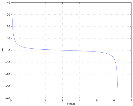
Figure 3: Plot of the function $f(\theta)$.

Furthermore, we will assume without loss of generality that $\theta\in(0,\pi)$ and hence we obtain our first design equation

$$\frac{\sin\theta}{1-\cos\theta}=\frac{|\epsilon|}{\sqrt{\kappa_{1}\kappa_{2}}}.$$ (102)

In practice, this ratio would be chosen in the range of $\frac{|\epsilon|}{\sqrt{\kappa_{1}\kappa_{2}}}\in(0,0.6)$ in order to ensure that the linearized model which is being used is valid.

We now construct the vectors $\alpha$ and $\beta$ so that condition (101) is satisfied. Indeed, we let

$$\alpha=\left[\begin{array}[]{l}1\\ \frac{\Re(\epsilon)-\Re(\delta)}{-\Im(\epsilon)-\Im(\delta)}\end{array}\right],~{}~{}\beta=\left[\begin{array}[]{l}-\Im(\epsilon)-\Im(\delta)\\ \Re(\epsilon)+\Re(\delta)\end{array}\right].$$

For these values of $\alpha$ and $\beta$, it is straightforward to verify that (101) is satisfied provided that $|\epsilon|=|\delta|$. With this value of $\beta$, we now calculate the quantity $e$ defined in (44) as follows:

$$e = \frac{4}{\kappa_{3}^{2}+16\omega_{o}^{2}}\left[\begin{array}[]{ll}\kappa_{3}&4\omega_{o}\\ -4\omega_{o}&\kappa_{3}\end{array}\right]J\beta$$

$$= -\frac{4}{\kappa_{3}^{2}+16\omega_{o}^{2}}\left[\begin{array}[]{ll}\kappa_{3}&4\omega_{o}\\ -4\omega_{o}&\kappa_{3}\end{array}\right]\left[\begin{array}[]{l}\Re(\epsilon)+\Re(\delta)\\ \Im(\epsilon)+\Im(\delta)\end{array}\right].$$

Then, the vector $K$ defining the quadrature measured by the homodyne detector is constructed according to the equation (46).

In the special case that $\omega_{o}=0$, this reduces to

$$e=-\frac{4}{\kappa_{3}}\left[\begin{array}[]{l}\Re(\epsilon)+\Re(\delta)\\ \Im(\epsilon)+\Im(\delta)\end{array}\right].$$

In terms of complex numbers ${\bf e}=e(1)+\imath e(2)$, we can write this as

$${\bf e}=-\frac{4}{\kappa_{3}}(\epsilon+\delta).$$

Then, in terms of complex numbers ${\bf K}=K(1)+\imath K(2)$, the formula (46) becomes

$${\bf K}=\frac{{\bf e}}{|{\bf e}|^{2}}=-\frac{\kappa_{3}(\epsilon+\delta)}{4(\epsilon+\delta)(\bar{\epsilon}+\bar{\delta})}=-\frac{\kappa_{3}}{4(\bar{\epsilon}+\bar{\delta})}$$

where $\bar{(\cdot)}$ denotes complex conjugate. Also, as noted in Section II, the steady state measurement noise intensity is given by

$$\frac{1}{\|e\|}=-\frac{\kappa_{3}}{4|\epsilon+\delta|}$$

which approaches zero as $\kappa_{3}\rightarrow 0$. However, this is at the expense of increasingly slower convergence to steady state.

IV Conclusions

In this paper, we have shown that a direct coupling observer for a linear quantum system can be implemented in the case that the observer can be measured using a Homodyne detection measurement. This would allow the plant observer system to be constructed experimentally and the performance of the observer could be verified using the measured data.

References

[1]
Z. Miao and M. R. James, “Quantum observer for linear quantum stochastic
systems,” in Proceedings of the 51st IEEE Conference on Decision and
Control, Maui, December 2012.
[2]
I. Vladimirov and I. R. Petersen, “Coherent quantum filtering for physically
realizable linear quantum plants,” in Proceedings of the 2013 European
Control Conference, Zurich, Switzerland, July 2013, arXiv:1301.3154.
[3]
Z. Miao, L. A. D. Espinosa, I. R. Petersen, V. Ugrinovskii, and M. R. James,
“Coherent quantum observers for finite level quantum systems,” in
Australian Control Conference, Perth, Australia, November 2013.
[4]
I. R. Petersen, “A direct coupling coherent quantum observer,” in
Proceedings of the 2014 IEEE Multi-conference on Systems and Control,
Antibes, France, October 2014, also available arXiv 1408.0399.
[5]
——, “A direct coupling coherent quantum observer for a single qubit finite
level quantum system,” in Proceedings of 2014 Australian Control
Conference, Canberra, Australia, November 2014, also arXiv 1409.2594.
[6]
——, “Time averaged consensus in a direct coupled distributed coherent
quantum observer,” in Proceedings of the 2015 American Control
Conference, Chicago, IL, July 2015.
[7]
——, “Time averaged consensus in a direct coupled coherent quantum observer
network for a single qubit finite level quantum system,” in
Proceedings of the 10th ASIAN CONTROL CONFERENCE 2015, Kota Kinabalu,
Malaysia, May 2015.
[8]
I. R. Petersen and E. H. Huntington, “A possible implementation of a direct
coupling coherent quantum observer,” in Proceedings of 2015 Australian
Control Conference, Gold Coast, Australia, November 2015.
[9]
M. R. James, H. I. Nurdin, and I. R. Petersen, “ control of linear
quantum stochastic systems,” IEEE Transactions on Automatic Control,
vol. 53, no. 8, pp. 1787–1803, 2008, arXiv:quant-ph/0703150.
[10]
I. R. Petersen, “Quantum linear systems theory,” in Proceedings of the
19th International Symposium on Mathematical Theory of Networks and Systems,
Budapest, Hungary, July 2010.
[11]
H. I. Nurdin, M. R. James, and A. C. Doherty, “Network synthesis of linear
dynamical quantum stochastic systems,” SIAM Journal on Control and
Optimization, vol. 48, no. 4, pp. 2686–2718, 2009.
[12]
J. Gough and M. R. James, “The series product and its application to quantum
feedforward and feedback networks,” IEEE Transactions on Automatic
Control, vol. 54, no. 11, pp. 2530–2544, 2009.
[13]
G. Zhang and M. James, “Direct and indirect couplings in coherent feedback
control of linear quantum systems,” IEEE Transactions on Automatic
Control, vol. 56, no. 7, pp. 1535–1550, 2011.
[14]
H. Bachor and T. Ralph, A Guide to Experiments in Quantum Optics,
2nd ed. Weinheim, Germany: Wiley-VCH,
2004.
[15]
L. Mandel and E. Wolf, Optical Coherence and Quantum Optics. Cambridge, UK: Cambridge University Press, 1995.
[16]
A. J. Shaiju and I. R. Petersen, “A frequency domain condition for the
physical realizability of linear quantum systems,” IEEE Transactions
on Automatic Control, vol. 57, no. 8, pp. 2033 – 2044, 2012.