Abstract

The possibility of immunized and improving the entanglement of accelerated systems via local filtering is discussed. The maximum bounds of entanglement depend on the dimensions of the accelerated and the filtered subsystems. If the small dimensional subsystem is accelerated and the large dimensional subsystem is filtered, one can get a long-lived entanglement. Moreover, if the larger subsystem is accelerated, then by filtering any subsystem, the upper bounds of entanglement of the filtered state are larger then that for the initial states.For any accelerated subsystem, the entanglement always increases as the filter strength of the large dimensional subsystem increases.

Keyword: Entanglement, acceleration, Filtering, qutrit, qubit

1 Introduction

It is well known that, to perform quantum information tasks, maximum entangled states are required. Although, it is possible to generate such states, mainting their isolation is a very difficult task. There are many studies devoted to investigate the behavior of entanglement in different environments [2]. On the other hand, the possibility of using these noise states to perform some quantum information is studied from different point of views[3].

Due to the interaction with the environments the amount of entanglement decreases and accordingly their efficiency to perform quantum information tasks decreases. Therefore, it is a necessity to improve the weakness of entanglement. For this aim, there are different protocols of purifications that have been introduced [4, 5, 6, 7], where the main idea of these protocols is based on local quantum operations, classical communication and measurements. So, one can get a smaller numbers of strongly entangled qubits from a large number of weakly entangled ones. Bennett. et.al. [8], showed that local filtering can be used to increase the entanglement of a two-qubit by applying it on one of its subsystems. A single local filter operation can be used to retrieve the loss of entanglement of particles passing through noise channels [9]. Moreover local filtering is used to increase the entanglement of subsystem at the expense of the other subsystem [10]. The effect of local filtering on the dynamics of some measures of quantum correlation of a general two qubit state is discusses by Karmakar et. al, [11].

Some efforts have been done recently to investigate the survival amount of entanglement between different accelerated systems [12]. These accelerated states can be used to perform some quantum information tasks such as teleportation [13] and quantum coding [14]. Due to the acceleration, the entanglement between the accelerated partners decreases, where the decay rate depends on the initial acceleration and the dimension of the accelerated subsystem. Therefore, it is worth to investigate, the possibility of improving the entanglement between the accelerated particles by filtering one of the subsystems. We introduce this idea by using a state composite of two different dimensional subsystems; qubit $(2D)$ and qutrit $(3D)$. This state is described by one parameter, known as one parameter family[15], where it is shown that, if the larger subsystem is accelerated the rate of entanglement decay is larger than that depicted for accelerating the small dimension subsystem [17].

This paper is organized as follows: In Sec.2, we define the qubit-qutrit state and its final form in the non-inertial frame when one or both particles are accelerated. The filtering process is discussed in Sec.3, where analytical solutions are obtained for the final filtered states. The degree of entanglement between the accelerated partner is quantified by using the negativity as a measure of entanglement. Finally, we summarize or results and conclusions in Sec. 4.

2 The suggested model

We consider a state that represents a class of qubit-qutrit system in $2\times 3$ dimensional and described by only one parameter. In the computation basis $00,01.02,10,11,12$, it takes the form

$$\rho = \Bigl{\{}\frac{\mu}{2}(\bigl{|}0\bigr{\rangle}_{b}\bigl{\langle}0\bigr{|}+\bigl{|}1\bigr{\rangle}_{b}\bigl{\langle}1\bigr{|})\Bigl{\}}\otimes\bigl{|}1\bigr{\rangle}_{t}\bigl{\langle}1\bigr{|}+\Bigl{\{}\frac{\mu}{2}\bigl{|}1\bigr{\rangle}_{b}\bigl{\langle}1\bigr{|}+\frac{1-2\mu}{2}\bigl{|}0\bigr{\rangle}_{b}\bigl{\langle}0\bigr{|}\Bigr{\}}\otimes\bigl{|}2\bigr{\rangle}_{t}\bigl{\langle}2\bigr{|}$$ (1)

$$+\Bigl{\{}\frac{\mu}{2}\bigl{|}0\bigr{\rangle}_{b}\bigl{\langle}1\bigr{|}+\frac{1-2\mu}{2}\bigl{|}1\bigr{\rangle}_{b}\bigl{\langle}0\bigr{|}\Bigr{\}}\otimes\bigl{|}0\bigr{\rangle}_{t}\bigl{\langle}2\bigr{|}+\Bigl{\{}\frac{\mu}{2}\bigl{|}1\bigr{\rangle}_{b}\bigl{\langle}0\bigr{|}+\frac{1-2\mu}{2}\bigl{|}0\bigr{\rangle}_{b}\bigl{\langle}1\bigr{|}\Bigr{\}}\otimes\bigl{|}2\bigr{\rangle}_{t}\bigl{\langle}0\bigr{|}$$

$$+\Bigl{\{}\frac{\mu}{2}\bigl{|}0\bigr{\rangle}_{b}\bigl{\langle}0\bigr{|}\Bigr{\}}\otimes\bigl{|}0\bigr{\rangle}_{t}\bigl{\langle}0\bigr{|}+\Bigl{\{}\frac{1-2\mu}{2}\bigl{|}1\bigr{\rangle}_{b}\bigl{\langle}0\bigr{|}\Bigr{\}}\otimes\bigl{|}0\bigr{\rangle}_{t}\bigl{\langle}1\bigr{|}$$

where, $0\leq\mu\leq\frac{1}{2}$ and the subscript $"b"$ refers to the qubit while $"t"$ refers to the qutrit [16, 17]

In what follows, we consider only one subsystem is accelerated. Accordingly we have the following cases:accelerated and filtered qubit, accelerated qubit and filtered qutrit, accelerated qutrit and filtered qubit and accelerated and filtered qutrit.

2.1 Accelerated the subsystems

First, we review the relation between Monkowski and Rindler spaces [18, 19]. For qubit systems, if the coordinates of a particle is defined by $(t,z)$ in Minkowski space, then in Rindlier space it is defined by $(\tau,x)$, where

$$\tau=r\tanh(t/z),\quad x=\sqrt{t^{2}-z^{2}},\quad-\infty<r<\infty,\quad-\infty<x<\infty.$$ (2)

Also, the annihilation operators $a_{ku}$ and $b_{-kU}$ in Minkowski space can be written by means of Rindler operators [20, 21] $(c_{kR}^{(I)},\quad d^{II}_{-kL})$ as,

$$a_{kU} = cosr_{b}c^{(I)}_{kR}-e^{-i\phi}\sin r_{b}d^{II}_{-KL},\quad$$

$$b^{\dagger}_{-kU} = e^{-i\phi}\sin r_{b}c^{(I)}_{kR}+\cos r_{b}d^{II}_{-KL},$$ (3)

where $\tan r_{b}=Exp[-\pi\omega\frac{c}{a}]$,  $0\leq r_{b}\leq\pi/4$, $-\infty\leq a\leq\infty$, $\omega$ is the frequency,$c$ is the speed of light, and $\phi$ is the phase space which can be absorbed in the definition of the operators[21]. The relations $(3)$, mix a particle in the region $I$ and its anti-particle in the region $II$ such that the computational basis $\bigl{|}0_{k}\bigr{\rangle}$and $\bigl{|}1_{k}\bigr{\rangle}$ can be written as[17],

$$\bigl{|}0_{k}\bigr{\rangle} = \cos r_{b}\bigl{|}0_{k}\bigr{\rangle}_{I}\bigl{|}0_{-k}\bigr{\rangle}_{II}+\sin r_{b}\bigl{|}1_{k}\bigr{\rangle}_{I}\bigl{|}1_{-k}\bigr{\rangle}_{II},$$

$$\bigl{|}1_{k}\bigr{\rangle} = a^{\dagger}_{k}\bigl{|}0_{k}\bigr{\rangle}=\bigl{|}1_{k}\bigr{\rangle}_{I}\bigl{|}0_{k}\bigr{\rangle}_{II}.$$ (4)

Now, for qutrit systems, the Minkowski vacuum state $\bigl{|}0_{m}\bigr{\rangle}$, spin up state $\bigl{|}\mathcal{U}\bigr{\rangle}$, spin down state $\bigl{|}\mathcal{D}\bigr{\rangle}$ and the pair state $\bigl{|}\mathcal{P}\bigr{\rangle}$, in the Rindler space are defined in [17, 22, 23] as

$$\bigl{|}0_{M}\bigr{\rangle} = \cos^{2}r_{t}\bigl{|}0\bigr{\rangle}_{I}\bigl{|}0\bigr{\rangle}_{II}+\frac{1}{2}e^{i\phi}\sin 2r_{t}(\bigl{|}\mathcal{U}\bigr{\rangle}_{I}\bigl{|}\mathcal{D}\bigr{\rangle}_{II}+\bigl{|}\mathcal{D}\bigr{\rangle}_{I}\bigl{|}\mathcal{U}\bigr{\rangle}_{II})+e^{2i\phi}sin^{2}r_{t}\bigl{|}\mathcal{D}\bigr{\rangle}_{I}\bigl{|}\mathcal{P}\bigr{\rangle}_{II},$$

$$\bigl{|}\mathcal{U}_{M}\bigr{\rangle} = \cos r_{t}\bigl{|}\mathcal{U}\bigr{\rangle}_{I}\bigl{|}0\bigr{\rangle}_{II}+e^{i\phi}\sin r_{t}\bigl{|}\mathcal{P}\bigr{\rangle}_{I}\bigl{|}\mathcal{U}\bigr{\rangle}_{II},$$

$$\bigl{|}\mathcal{D}_{M}\bigr{\rangle} = \cos r_{t}\bigl{|}\mathcal{D}\bigr{\rangle}_{I}\bigl{|}0\bigr{\rangle}_{II}-e^{i\phi}\sin r_{t}\bigl{|}\mathcal{P}\bigr{\rangle}_{I}\bigl{|}\mathcal{D}\bigr{\rangle}_{II}.$$ (5)

By using the initial state (1) and the transformations (4), one gets the final state of the accelerated system, where only the qubit is accelerated. After tracing out the mode in region $II$, the final accelerated state between Alice and Bob in the first region, $I$ can be written as,

$$\rho^{ac-b} = \mathcal{A}_{1}\bigl{|}00\bigr{\rangle}\bigl{\langle}00\bigr{|}+\mathcal{A}_{2}\bigl{|}01\bigr{\rangle}\bigl{\langle}01\bigr{|}+\mathcal{A}_{3}\bigl{|}00\bigr{\rangle}\bigl{\langle}12\bigr{|}+\mathcal{A}_{4}\bigl{|}12\bigr{\rangle}\bigl{\langle}00\bigr{|}$$ (6)

$$+\mathcal{A}_{5}\bigl{|}10\bigr{\rangle}\bigl{\langle}02\bigr{|}+\mathcal{A}_{6}\bigl{|}02\bigr{\rangle}\bigl{\langle}10\bigr{|}+\mathcal{A}_{7}\bigl{|}02\bigr{\rangle}\bigl{\langle}02\bigr{|}+\mathcal{A}_{8}\bigl{|}10\bigr{\rangle}\bigl{\langle}10\bigr{|}$$

$$+\mathcal{A}_{9}\bigl{|}12\bigr{\rangle}\bigl{\langle}12\bigr{|}+\bigl{|}11\bigr{\rangle}\bigl{\langle}11\bigr{|}$$

where,

$$\mathcal{A}_{1} = \mathcal{A}_{2}=\frac{\mu}{2}\cos^{2}r_{b},\quad\mathcal{A}_{3}=\mathcal{A}_{4}=\frac{\mu}{2}\cos r_{b},$$

$$\mathcal{A}_{5} = \mathcal{A}_{6}=\frac{1-2\mu}{2}\cos r_{b},\quad\mathcal{A}_{7}=\frac{1-2\mu}{2}\cos^{2}r_{b},$$

$$\mathcal{A}_{8} = \frac{1-2\mu}{2}+\frac{\mu}{2}\sin^{2}r_{b},\quad\mathcal{A}_{9}=\frac{\mu}{2}+\frac{1-2\mu}{2}\sin^{2}r_{b},\quad\mathcal{A}_{10}=\frac{\mu}{2}(1+\sin^{2}r_{b}).$$ (7)

Similarly, to accelerate the qutrit one uses the transformation (5) and the initial state (1). However by tracing out the mode in $II$, the final accelerated state between the partners in the first region takes the form,

$$\rho^{ac-t} = \mathcal{B}_{1}\bigl{|}00\bigr{\rangle}\bigl{\langle}00\bigr{|}+\mathcal{B}_{2}\bigl{|}01\bigr{\rangle}\bigl{\langle}01\bigr{|}+\mathcal{B}_{3}\bigl{|}02\bigr{\rangle}\bigl{\langle}02\bigr{|}+\mathcal{B}_{4}\bigl{|}0\mathcal{P}\bigr{\rangle}\bigl{\langle}0\mathcal{P}\bigr{|}$$

$$+\mathcal{B}_{5}\bigl{|}10\bigr{\rangle}\bigl{\langle}10\bigr{|}+\mathcal{B}_{6}\bigl{|}11\bigr{\rangle}\bigl{\langle}11\bigr{|}+\mathcal{B}_{7}\bigl{|}12\bigr{\rangle}\bigl{\langle}12\bigr{|}+\mathcal{B}_{8}\bigl{|}1\mathcal{P}\bigr{\rangle}\bigl{\langle}1\mathcal{P}\bigr{|}$$

$$+\mathcal{B}_{9}\bigl{|}12\bigr{\rangle}\bigl{\langle}00\bigr{|}+\mathcal{B}_{10}\bigl{|}1\mathcal{P}\bigr{\rangle}\bigl{\langle}01\bigr{|}+\mathcal{B}_{11}\bigl{|}02\bigr{\rangle}\bigl{\langle}10\bigr{|}+\mathcal{B}_{12}\bigl{|}0\mathcal{P}\bigr{\rangle}\bigl{\langle}11\bigr{|}$$

$$+\mathcal{B}_{13}\bigl{|}00\bigr{\rangle}\bigl{\langle}12\bigr{|}+\mathcal{B}_{14}\bigl{|}01\bigr{\rangle}\bigl{\langle}1\mathcal{P}\bigr{|}+\mathcal{B}_{15}\bigl{|}10\bigr{\rangle}\bigl{\langle}02\bigr{|}+\mathcal{B}_{16}\bigl{|}11\bigr{\rangle}\bigl{\langle}0\mathcal{P}\bigr{|}$$

where,

$$\mathcal{B}_{1} = \frac{\mu}{2}\cos^{4}r_{t},\quad\mathcal{B}_{2}=\frac{\mu}{2}\cos^{2}r_{t}(1+\sin^{2}r_{t}),\quad\mathcal{B}_{3}=\frac{\mu}{8}\sin^{2}2r_{t},\quad$$

$$\mathcal{B}_{4} = \sin^{2}r_{t}\left(\frac{p}{2}\sin^{2}r_{t}+\frac{1-2\mu}{2}\right),\quad\mathcal{B}_{5}=\frac{1-2\mu}{2}\cos^{4}r_{t},\quad\mathcal{B}_{6}=\cos^{2}r_{t}\left(\frac{\mu}{2}+\frac{1-2\mu}{2}\sin^{2}r_{t}\right),\quad$$

$$\mathcal{B}_{7} = \frac{1-2\mu}{8}\sin^{2}2r_{t},\quad\mathcal{B}_{8}=\sin^{2}r_{t}\left(\frac{\mu}{2}+\frac{1-2\mu}{2}\sin^{2}r_{t}\right),\quad\mathcal{B}_{9}=\frac{\mu}{2}\cos^{3}r_{t},\quad\quad$$

$$\mathcal{B}_{10} = \frac{\mu}{4}\sin 2r_{t}\sin r_{t},\quad\mathcal{B}_{11}=\frac{1-2\mu}{2}\cos^{2}r_{t},\quad\mathcal{B}_{12}=\frac{1-2\mu}{4}\sin 2r_{t}\sin r_{t},\quad\$$

$$\mathcal{B}_{13} = \mathcal{B}_{9},\quad\mathcal{B}_{14}=\mathcal{B}_{10},\quad\mathcal{B}_{15}=\mathcal{B}_{11},\quad\mathcal{B}_{16}=\mathcal{B}_{12}.$$ (9)

The entanglement is quantified by using the negativity as a measure, where for a system consists of two different dimensions as qubit and qutrit, the negativity of a bipartite system consists of two subsystems have dimensions $d_{1}$ and $d_{2}$,$(d_{1}<d_{2})$ is given by

$${\Large\mathcal{E}}=\frac{1}{d_{1}-1}\Bigl{\{}||\rho^{T_{2}}_{ab}||-1\Bigr{\}},$$ (10)

where $\rho^{T_{b}}_{ab}$ is the partial transpose with respect to the largest dimension subsystem and $||.||$ is the trace norm[15, 24].

3 Filtering process

In this section, we investigate the effect of the local filter operation on the behavior of the degree of entanglement. For qubit system the filter operation is defined by a non-trace preserving operator [25, 9]. In the computational basis the filter operator $\mathcal{F}_{b}$ can be described by

$$\mathcal{F}_{b}=\sqrt{\kappa}\bigl{|}0\bigr{\rangle}\bigl{\langle}0\bigr{|}+\sqrt{1-\kappa}\bigl{|}1\bigr{\rangle}\bigl{\langle}1\bigr{|}$$ (11)

where, $0<\kappa<1$. Let us assume that the accelerated state is given by $\rho^{ac-q_{i}}$, where $i=b,t$. If the qubit is filtered then the filtered state is given by [9, 26]

$$\rho_{b-F}^{ac-q_{i}}=\frac{1}{\mathcal{N}_{b}}\Bigl{(}\mathcal{F}_{b}\otimes I_{3\times 3}\Bigr{)}\rho^{ac-q_{i}}\Bigl{(}\mathcal{F}^{\dagger}_{b}\otimes I_{3\times 3}\Bigr{)}$$ (12)

where $\mathcal{N}_{b}={\mathrm{tr}_{\,}\left\{\Bigl{(}\mathcal{F}_{b}\otimes I_{3\times 3}\Bigr{)}\rho^{ac-q_{i}}\Bigl{(}\mathcal{F}^{\dagger}_{b}\otimes I_{3\times 3}\Bigr{)}\right\}}$ is a normalization factor. For qutrit system the filter operator is defined by [27]

$$\mathcal{F}_{t}^{(1)} = \bigl{|}0\bigr{\rangle}\bigl{\langle}0\bigr{|}+\sqrt{1-\mathcal{Q}}\bigl{|}1\bigr{\rangle}\bigl{\langle}1\bigr{|}+\sqrt{\mathcal{Q}}\bigl{|}2\bigr{\rangle}\bigl{\langle}2\bigr{|},$$

$$\mathcal{F}_{t}^{(2)} = \sqrt{\mathcal{Q}}\bigl{|}1\bigr{\rangle}\bigl{\langle}1\bigr{|}+\sqrt{1-\mathcal{Q}}\bigl{|}2\bigr{\rangle}\bigl{\langle}2\bigr{|}.$$ (13)

If Bob applies the filter operation on his particle then the output state is given by

$$\rho_{t-F}^{ac-q_{i}}=\frac{1}{\mathcal{N}_{t}}\sum_{j=1}^{2}\Bigl{(}I_{2\times 2}\otimes\mathcal{F}^{(j)}_{t}\Bigr{)}\rho^{ac-q_{i}}\Bigl{(}I_{2\times 2}\otimes\mathcal{F}^{\dagger(j)}_{t}\Bigr{)}$$ (14)

where the normalization factor is $\mathcal{N}_{t}={\mathrm{tr}_{\,}\left\{\sum_{j=1}^{2}\Bigl{(}I_{2\times 2}\otimes\mathcal{F}^{(j)}_{t}\Bigr{)}\rho^{ac-q_{i}}\Bigl{(}I_{2\times 2}\otimes\mathcal{F}^{\dagger(j)}_{t}\Bigr{)}\right\}}$, $j=1,2$.

3.1 Alice’ s qubit is accelerated

• Alice’s qubit is filtered
  For this case, it is assumed that only Alice filters her qubit by applying the operator (11). The final filtered state is given by,

  $$\rho^{ac-b}_{b-F} = \frac{1}{\mathcal{N}_{b-F}}\Bigl{\{}\kappa\left(A_{1}\bigl{|}00\bigr{\rangle}\bigl{\langle}00\bigr{|}+A_{2}\bigl{|}01\bigr{\rangle}\bigl{\langle}01\bigr{|}+A_{7}\bigl{|}02\bigr{\rangle}\bigl{\langle}02\bigr{|}\right)$$ (15)

  $$+(1-\kappa)(A_{8}\bigl{|}10\bigr{\rangle}\bigl{\langle}10\bigr{|}+A_{9}\bigl{|}12\bigr{\rangle}\bigl{\langle}12\bigr{|}+A_{10}\bigl{|}11\bigr{\rangle}\bigl{\langle}11\bigr{|})$$

  $$+\sqrt{\kappa}\sqrt{1-\kappa}\left(A_{3}\bigl{|}00\bigr{\rangle}\bigl{\langle}12\bigr{|}+A_{4}\bigl{|}12\bigr{\rangle}\bigl{\langle}00\bigr{|}+A_{5}\bigl{|}10\bigr{\rangle}\bigl{\langle}02\bigr{|}+A_{6}\bigl{|}02\bigr{\rangle}\bigl{\langle}10\bigr{|}\right)\Bigr{\}}$$

  where, the coefficients $\mathcal{A}_{i},i=1..10$ are given by (7) and the normalized factor is

  $$\mathcal{N}_{b-F}=\kappa\left(\mathcal{A}_{1}+\mathcal{A}_{2}+\mathcal{A}_{7}\right)+(1-\kappa)\left(\mathcal{A}_{8}+\mathcal{A}_{9}+\mathcal{A}_{10}\right).$$

  

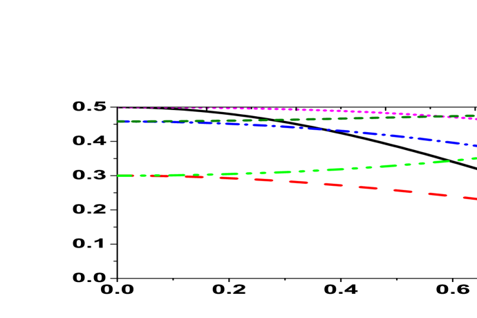
  Figure 1: The entanglement of the filtered accelerated state against the acceleration, where only the qubit is accelerated. The dash, dash-dot,dot short dash and dash-dot-dot curves for $\kappa=0.1,0.3,0.5,0.7,0.9$, respectively, while the solid curve for the non-filtered state.

  Fig.(1), describes the behavior of entanglement of the accelerated system between Alice and Bob after performing the filtering process, where different values of the filtering strengths are considered. The effect of the filtering parameter $\kappa$,( only Alice qubit is filtered), on the degree of entanglement is investigated. It is clear that, for small values of $\kappa$, the initial degree of entanglement ($r_{b}=0$) is smaller than that depicted for the non-filtered case (solid-curve). However, as one increases $\kappa\in[0,0.5]$, the decay rate of entanglement decreases and consequently the lower bounds of entanglement increase. Moreover, for $\kappa=0.5$ the upper bound of entanglement is larger than that displayed for the non-filtered case. This behavior is changed dramatically for $\kappa\in(0.5,1)$, where the initial degree of entanglement is smaller than that shown for the non-filtered case. As $r_{b}$ increases, the entanglement increases and when the acceleration goes to infinity, the entanglement is much better than the non-filtered case.

• Bob’s qutrit is filtered
  In this case, the final state is given by

  $$\rho^{b-ac}_{t-F} = \frac{1}{N_{t-F}}\Bigl{\{}A_{1}\bigl{|}00\bigr{\rangle}\bigl{\langle}00\bigr{|}+A_{2}\bigl{|}01\bigr{\rangle}\bigl{\langle}01\bigr{|}+A_{3}\bigl{|}02\bigr{\rangle}\bigl{\langle}02\bigr{|}$$ (16)

  $$+A_{4}\bigl{|}10\bigr{\rangle}\bigl{\langle}10\bigr{|}+A_{5}\bigl{|}11\bigr{\rangle}\bigl{\langle}11\bigr{|}+A_{6}\bigl{|}12\bigr{\rangle}\bigl{\langle}12\bigr{|})$$

  $$+\sqrt{q}\left(A_{7}\bigl{|}00\bigr{\rangle}\bigl{\langle}12\bigr{|}+A_{8}\bigl{|}02\bigr{\rangle}\bigl{\langle}10\bigr{|}+A_{9}\bigl{|}12\bigr{\rangle}\bigl{\langle}00\bigr{|}+A_{10}\bigl{|}10\bigr{\rangle}\bigl{\langle}02\bigr{|}\right)\Bigr{\}}$$

  where, $A_{i},i=1..10$ are given by (7) and the normalization factor $N_{t-F}=\sum_{i=1}^{6}A_{i}$

  

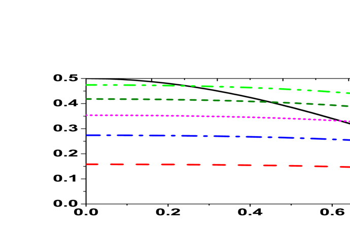
  Figure 2: The sam as Fig.(1) but it is assumed that the qutrit is filtered. The dash, dash-dot, dot short dash and dash-dot-dot curves for $\mathcal{Q}=0.1,0.3,0.5,0.7$ and $0.9$, respectively, and the sold curve for the n non-filtered case.

  Fig.(2) shows the behavior of entanglement when Bob’s particle (qutrit) is filtered. It is clear that, for small values of the filtering parameter $\mathcal{Q}$, the initial degree of entanglement is smaller than that depicted for the non-filtered case (solid curve). As one increases $\mathcal{Q}$, the entanglement increases and slightly degreases at $r_{b}\to\infty$. However for $\mathcal{Q}\in(0.3,1)$, the upper bounds of entanglement at $r_{b}\to\infty$ are always larger compared with the non-filtered case. It is clear that, the entanglement can be immunized from decaying by applying the filtering at the decreasing points. For example, at $r_{b}\sim 0.6$, the entanglement decay can be prevented, if the qutrit is filtered with a strength $\mathcal{Q}=0.5$.

  From Figs.(1) and (2) one can concludes that, local filtering can improve the degree of entanglement for the accelerating systems. The long lived entanglement can be displayed if the qutrit is filtered for any values of the strength’s filter $\mathcal{Q}$. For some particular values of $\kappa$ one can obtain a long-lived entanglement. If the qubit is filtered, the entanglement increases for $r_{b}\to\infty$, while it slightly decreases if the qutrit is filtered. Therefore, if the smaller dimensional subsystem is accelerated and the larger dimensional subsystem is filtered, one obtains a long-lived entanglement between the partners. Moreover, local filtering, not only can be used to immunize the entanglement but also can be used to improve it. So, it can be considered as a resource of quantum purification to improve the efficiency of the accelerated state.

  

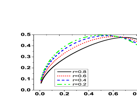
  Figure 3: The amount of entanglement the strength of the filter $k$ for different values of the acceleration $r_{b}=r=0.8,0.6.0.4$ and $0.2$ .

  In Fig.(3), we investigate the behavior of entanglement against the filtering strengths $\kappa$ and $\mathcal{Q}$, where different values of $r_{b}$ are considered. In Fig.(3a), the maximum values of entanglement depend on the initial acceleration and the strength of the filter. For small accelerations the upper bounds of entanglement at a fixed values of $\kappa\in(0,0.5)$ are much larger than those depicted for larger acceleration. This behavior is changed for larger values of $\kappa\in(0.5,1)$, where the larger acceleration, the smaller upper bounds of entanglement. Fig.(3b), shows the effect of qutrit’s filter strength $\mathcal{Q}$ on the degree of entanglement for different values of the accelerations. It is clear that, the entanglement $\mathcal{E}$ increases as $\mathcal{Q}$ increases and its upper bounds that depend on the initial acceleration, where they are small for larger accelerations’s values.

  

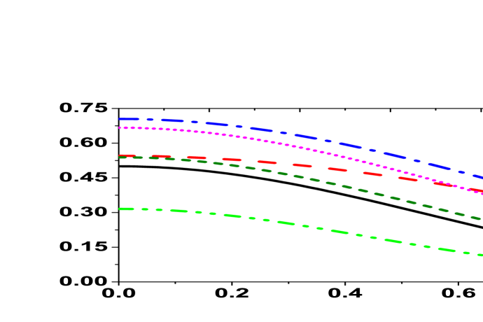
  Figure 4: The same as Fig.(1) but only the qutrit is accelerated.

  3.2 Bob’s qutrit is accelerated

  In this case, the final state between Alice and Bob is given by Eq.(8). We consider the following possibilities:

• Alice ’s qubit is filtered
  For this case Alice uses the filter defined by Eq.(11) to filter her qubit. After finishing the filtering process, the partners Alice and Bob share the following state.

  $$\rho^{t-ac}_{b-F} = \frac{1}{\tilde{N}_{b-F}}\Bigl{\{}\kappa(\mathcal{B}_{1}\bigl{|}00\bigr{\rangle}\bigl{\langle}00\bigr{|}+\mathcal{B}_{2}\bigl{|}01\bigr{\rangle}\bigl{\langle}01\bigr{|}+\mathcal{B}_{3}\bigl{|}02\bigr{\rangle}\bigl{\langle}02\bigr{|})$$ (17)

  $$+(1-\kappa)(\mathcal{B}_{4}\bigl{|}10\bigr{\rangle}\bigl{\langle}10\bigr{|}+\mathcal{B}_{5}\bigl{|}11\bigr{\rangle}\bigl{\langle}11\bigr{|}+\mathcal{B}_{6}\bigl{|}12\bigr{\rangle}\bigl{\langle}12\bigr{|})$$

  $$+\sqrt{\kappa}\sqrt{1-\kappa}(\mathcal{B}_{7}\bigl{|}02\bigr{\rangle}\bigl{\langle}10\bigr{|}+\mathcal{B}_{8}\bigl{|}10\bigr{\rangle}\bigl{\langle}02\bigr{|}+\mathcal{B}_{9}\bigl{|}12\bigr{\rangle}\bigl{\langle}00\bigr{|}+\mathcal{B}_{10}\bigl{|}00\bigr{\rangle}\bigl{\langle}12\bigr{|})\Bigr{\}}$$

  where, $\mathcal{B}_{i}$ are given by (9) and the normalized factor is defined as,

  $$\tilde{N}_{b-F}=\kappa\sum_{i=1}^{3}\mathcal{B}_{i}+(1-\kappa)\sum_{i=4}^{6}\mathcal{B}_{i}$$

  Fig(4) describes the behavior of entanglement if the qutrit is accelerated and the qubit is filtered. It is clear that, the initial degree of entanglement of the accelerated state is much better than the non-filtering case for $0<\kappa<0.7$. The upper bounds of $\mathcal{E}$ are lager for $\kappa<0.5$. However for farther values of $\kappa$ the upper bounds of entanglement decrease. For larger values of $\kappa>0.8$, the degree of entanglement is smaller than that displayed for the non-filtered case (solid curves).

• Bob’s qutrit is filtered
  In this case we assume that only Bob particle (qutrit) is accelerated and has the ability to filter it. The final state of these two operations is given by,

  $$\rho^{q_{t}-ac}_{t-F} = \frac{1}{\tilde{N}_{t-F}}\Bigl{\{}B_{1}\bigl{|}00\bigr{\rangle}\bigl{\langle}00\bigr{|}+B_{2}\bigl{|}01\bigr{\rangle}\bigl{\langle}01\bigr{|}+B_{3}\bigl{|}02\bigr{\rangle}\bigl{\langle}02\bigr{|}+B_{4}\bigl{|}10\bigr{\rangle}\bigl{\langle}10\bigr{|}+B_{5}\bigl{|}11\bigr{\rangle}\bigl{\langle}11\bigr{|}$$ (18)

  $$+\sqrt{q}(B_{7}\bigl{|}02\bigr{\rangle}\bigl{\langle}10\bigr{|}+B_{8}\bigl{|}10\bigr{\rangle}\bigl{\langle}02\bigr{|}+B_{9}\bigl{|}12\bigr{\rangle}\bigl{\langle}00\bigr{|}+B_{10}\bigl{|}00\bigr{\rangle}\bigl{\langle}12\bigr{|})\Bigr{\}}$$

  where $B_{i},i=...10$ are given by (6) and $\tilde{N}_{t-F}=\sum_{i=1}^{5}\mathcal{B}_{i}$

  

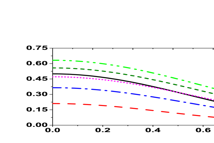
  Figure 5: The same as Fig.(2) but it is assumed only the qutrit is accelerated.

  In Fig.(5), the effect of the filtered qutrit on the entanglement of the accelerated state is investigated. It is clear that, the entanglement increases as the filtering strength $\mathcal{Q}$ increases. For small values of $\mathcal{Q}\in(0,~{}0.5)$, the filter process can not improve $\mathcal{E}$. However, for small range of $r_{t}\in(0.45,8)$ the entanglement can be improved if we set $\mathcal{Q}=0.5$. Moreover for any value of $\mathcal{Q}\in(0.5,1)$ the degree of entanglement is much better than that shown for the non filtered case (solid curve).

  

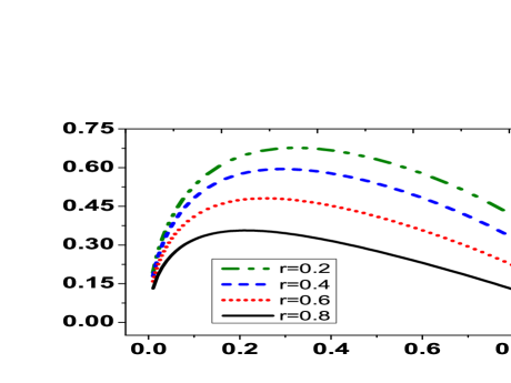
  Figure 6: The survival amount of entanglement for one parameter family against Filtering parameter (a) qubit filter strength, $\kappa$ and (b) qutrit filter strength $\mathcal{Q}$.

  Fig.(6) describes the behavior of entanglement against the filter’s strengths, where we consider some fixed values of the accelerations $r_{t}$. If only the qubit is filtered, one can see that the entanglement increases as $\kappa$ increases in intervals depending on the initial value of the accelerations. The maximum values of entanglement are large for small values of the acceleration. However, for further values of $\kappa$, the entanglement decreases. These phenomena can be seen in Fig.(6a). Meanwhile, if the qutrit is filtered, the entanglement increases as $\mathcal{Q}$ increases. Also, the maximum values of $\mathcal{E}$ are reached for small values of $r_{t}$ as shown in Fig.(6b).

  From Figs.(1) and (5), one can conclude that: it is possible to improve the entanglement between the partners if one user has accelerated his(her) subsystem. The improvement of the degree of entanglement depends on the initial acceleration, where for small accelerations one can improve it by controlling the filtering strength. For fixed accelerations, the maximum values of the entanglement can be reached as one increases the qutrit’s filter strength. The longed lived entanglement can be obtained if the smaller dimension subsystem (qubit) is accelerated and the larger dimensional subsystem (qutrit) is filtered. If the qutrit is accelerated one can increase the initial entanglement by filtering either the qubit or the qutrit. Meanwhile, the initial entanglement can not be increased if the small dimension subsystem (qubit )is accelerated and either the qubit or the qutrit is filtered.

  Comparing Figs.(3) and (6), we can see that for any subsystem accelerated the entanglement can be increased as the qutrit’s filter strength is increased. On the other hand, if any subsystem is accelerated and Alice has the ability to filter her qubit, then the maximum values of entanglement depend on the initial acceleration and the values of the qubit’s filter strength

4 Conclusion

In this contribution, the possibility of improving the entanglement of an accelerated state consists of two different dimensional subsystems is investigated. A state composed of qubit (two-dimensional) and qutrit (three dimensional) is considered to illustrate this idea . This state is described by only one parameter and it is known one-parameter family. Different cases are considered, where it is assumed that only one particle is accelerated. The final state in Minkowski space is obtained analytically for all cases. To improve the entanglement or decreasing the rate of entanglement decay, we consider only one filtered subsystem (qubit/qutrit).

In this context, it assumed that only one of the subsystem is accelerated, while the filtering process is performed on the qubit (small dimension subsystem) or the qutrit (large dimension subsystem), the qubit. It is shown that, local filtering can increase the upper bounds of entanglement of the accelerated system. The maximum bounds of entanglement depend on the values of the acceleration, filters’ strengths and the dimensions of the subsystem which is accelerated/filtered.

The obtained results show that, for a fixed acceleration of the qubit (small dimension subsystem), the entanglement of the filtered state increases as the qutrit’s filter strength increases, whilst if the qubit is filtered, then the entanglement increases over an interval of the strength depending on the initial acceleration. However, for larger values of the qubit’s filter strength, the entanglement of the large initial accelerations increases. On the other hand, if the qutrit is accelerated, then the increasing rate of entanglement at fixed values of accelerations is much larger than that depicted for the previous case (the qubit is accelerated). The larger values of entanglement’s bounds are drown for larger values of the qutrit’s filter strength, while they are seen for smaller values of the qubit’s filter strength

If the smallest dimension subsystem is accelerated, then the entanglement can not increase its initial values. One the other hand, for smaller acceleration, the entanglement bounds of the filtered state are much larger than those compared with a large acceleration. If the smaller dimensional subsystem is accelerated and filtered, the maximum entanglement of the filtered state depends on the initial acceleration and the value of the filter strength. Meanwhile, for accelerated qubit, one can obtain a long lived entanglement between the accelerated partners, where its upper bounds always increase as the filter strength of the qutrit increases.

In conclusion: local filtering can be considered as a resource of purifying the accelerated states, where it is possible to retrieve the lost entanglement. Local filtering play the same role played by the weak measurements to improve the entanglement. For noise environment, local filtering has the ability to retrieve the lost entanglement parabolisticaly, while for accelerated system in addition to retrieve the lost entanglement, it can increase it. If the smallest dimension subsystem is accelerated, one can not only recoup the lost entanglement but also a long-lived entanglement can be generated by filtering the larger dimension subsystem. However, if the largest subsystem is accelerated, one can in addition to retrieving the lost entanglement, increase the upper bounds of entanglement by filtering any subsystem (qubit/qutrit).

References

- [1] M. A. Nielsen, I. L. Chuang” Quantum Computation and Quantum Information”, ( Cambradge University Press), Cambridge (2000)
- [2] T. Yu and J. H. Eberly,”Sudden Death of Entanglement: Classical Noise Effects”, Opt. Commu.264 393 (2006); M. Yonac, T. Yu and J. H. Eberly,”Sudden Death of Entanglement of Two Jaynes-Cummings Atoms”, J. Phys. B 39 S621 (2006).
- [3] N. Metwally, ”Abruption decay of entanglement and quantum communication through noise channels”,Quantum information processing, 9 429-440 (2009);A. El Allati, N. Metwally, Y. Hassouni”, Transfer information remotely via noise entangled coherent channels”,Optics Communications, 284, 519-526 (2011).
- [4] C.H. Bennett, G. Brassard, S. Popescu, B. Schumacher, J.A. Smolin, W.K. Wootters,”Purification of Noisy Entanglement and Faithful Teleportation via Noisy Channels”, Phys. Rev. Lett. 76 722 (1996).
- [5] D. Deutsch, A. Ekert, R. Jozsa, C. Macchiavello, S. Popescu, A. Sanpera,”Quantum Privacy Amplification and the Security of Quantum Cryptography over Noisy Channels”, Phys. Rev. Lett. 77 2818 (1996)
- [6] N. Metwally,”More efficient entanglement purification”, Phys. Rev. A 66 054302 (2002).
- [7] N. Metwally, A.-S. Obada, ”More efficient purifying scheme via controlled controlled NOT gate”, Physics Letters A 352 45 (2006).
- [8] C. H. Bennett, H. J. Bernstein, S. Popescu, B. Schumacher,” Concentrating Partial Entanglement by Local Operations”, Phys.Rev.A 53:2046 (1996).
- [9] M. Siomau and A. Kamli,” Defeating entanglement sudden death by a single local filtering”, Phys. Rev. A 86 032304 (2012).
- [10] K. O. Yashodamma, P. J. Geetha and Sudha, ”Purification and redistribution of entanglement via single local filtering”, Int. J. Quantum Inf. 12 1450004 (2014).
- [11] S. Karmakar, A. Sen. A. Bhar and D. Sarkar, ” Effect of local filtering on freezing phenonena of quantum correlation”, Quantum Inform Processing 14 2517 (2015)
- [12] J. Wang and J. Jing, Phys. Rev. A. 83 022314 (2011); H. M.-Dehnavi, B. Mirza, H. Mohammadzadeh and R. Rahimi, Annals of Phys. 326 132 (2011).
- [13] N. Metwally” Telelportation of accelerated Information” J. Opt. Soci. Am B 30 233 (2013).
- [14] N. Metwally and A. Sagheer” Quantum coding in non-inertial frames”, Quantum Information Processing 13 771 (2014).
- [15] K. Ann, G. Jaeger, ”Entanglement sudden death in qubit-qutrit systems”, Phys. Lett. A372 579 (2008).
- [16] J.-L. Guo, J.-L. Wei and W. Qin, ” Enhancement of quantum correlations in qubit qutrit system under decoherence of finite temperature”,Quantum Inf Process 14 1399 1410 (2015).
- [17] N. Metwally,” Entanglement of simultaneous and non-simultaneous accelerated qubit-qutrit systems”, Quantum Inf. and Comput (QIC), 16 0530-0542 (2016).
- [18] E. M.-Martinez, I. Fuentes,”Redistribution of particle and antiparticle entanglement in noninertial frames”, Phys. Rev. A 83, 052306 (2011).
- [19] D. F. Walls and G. J. Milburn,”Quantum Optics”, Springer-Verlag, N. Y., (1994).
- [20] D. E. Bruschi, J. Louko, E. Martn-Martnez, A. Dragan, and I. Fuentes,”Unruh effect in quantum information beyond the single-mode approximation”, Phys. Rev. A 82 042332 (2010).
- [21] J. Doukas, E. G. Brown, A. J. Dragan, and R. B. Mann, ”Entanglement and discord: Accelerated observations of local and global modes”, Phys. Rev. A 87, 012306 (2013).
- [22] P. Alsing D. McMahon and G. Milburn, J. Opt. B:Quantum Seemiclass Opt. 6 S834-S843 (2004).
- [23] J. Len and E. M.-Martnez,”Spin and occupation number entanglement of Dirac fields for noninertial observers”, Phys. Rev. A 80 012314 (2009).
- [24] G. Karpat and Z. Gedik, Phys. Lett. A 375 4166-4171 (2011).
- [25] H. Hofmann and S. Takeuchi, ”Quantum Filter for Nonlocal Polarization Properties of Photonic Qubits”, Phys. Rev. Lett. 88 147901 (2002).
- [26] E. Hirsch, M. T. Quintino, J. Bowles and N. Brunner,” Genuine hidden quantum nonlocality” Phys. Rev. Lett. 111 160402 (2013).
- [27] Y. Kinoshita, R. Namiki, T. Yamamoto, M. Koashi and N. Imoto,”Selective entanglement breaking”, Phys. REv. A 75 032307 (2007).