Dynamic heterogeneity in two-dimensional supercooled liquids: comparison of bond-breaking and bond-orientational correlations

Abstract

We compare the spatial correlations of bond-breaking events and bond-orientational relaxation in a model two-dimensional liquid undergoing Newtonian dynamics. We find that the relaxation time of the bond-breaking correlation function is much longer than the relaxation time of the bond-orientational correlation function and self-intermediate scattering function. However, the relaxation time of the bond-orientational correlation function increases faster with decreasing temperature than the relaxation time of the bond-breaking correlation function and the self-intermediate scattering function. Moreover, the dynamic correlation length that characterizes the size of correlated bond-orientational relaxation grows faster with decreasing temperature than the dynamic correlation length that characterizes the size of correlated bond-breaking events. We also examine the ensemble-dependent and ensemble-independent dynamic susceptibilities for both bond-breaking correlations and bond-orientational correlations. We find that for both correlations, the ensemble-dependent and ensemble-independent susceptibilities exhibit a maximum at nearly the same time, and this maximum occurs at a time slightly shorter than the peak position of the dynamic correlation length.

1 Introduction

One of the most studied features of glassy dynamics is the existence of transient domains in which particles move in a correlated fashion, either much farther or much less than expected from a Gaussian distribution of displacements [1]. A connection between this dynamic heterogeneity and the structure was established in studies of the isoconfigurational ensemble in two-dimensions [2]. In these studies the same initial structure was used in many simulation runs, with the velocities chosen randomly from a Boltzmann distribution. It was found that there were regions where the particles were more likely to move farther than in other regions, and thus some aspects of the local structure were associated with the domains of heterogeneous dynamics. The exact nature of these aspects of the local structure is, however, not clear.

Recently it has been shown that there is a large difference in the growth of the characteristic size of dynamically heterogeneous regions upon supercooling in two and three dimensions if one defines dynamic heterogeneity through particle displacements [3]. This difference is mirrored in strong finite size effects in the quantities that probe translational motion of the tagged particle, e.g. the self-intermediate scattering function and the mean-square displacement, in two-dimensional glass forming liquids. Despite the difference in the tagged particle dynamics, there may be other dynamic observables that exhibit similar behavior in two and three dimensions. One can gain insight into potential observables that might exhibit similar behavior when one considers the dimensional dependence of the formation of ordered solids [4]. Similar to the glass transition, this freezing transition is also a transition from a liquid state where the shear modulus is zero, to a state with non-zero shear modulus. In three dimensions long-range translational and rotational order emerges when an ordered solid forms, but in two dimensions only long-range rotational order emerges when an ordered solid forms. Thus, in two-dimensional ordered solids, bond-orientational order should be monitored to look for the emergence of an elastic solid. When comparing the glass transition in two and three dimensions one may want to examine quantities that are expected to be similar in studies of the formation of two-dimensional and three-dimensional ordered solids, and this leads to examining correlations between bonds connecting neighboring particles.

Yamamoto and Onuki [5, 6] examined spatial correlations of bond-breaking events in a two-dimensional glassy binary mixture. They found large regions in which bond-breaking events were correlated by examining four-point structure factors in which the so-called weight function [7] was determined by bond-breaking events. Subsequently, Shiba, Kawasaki, and Onuki [8] compared bond-breaking correlations and mobility correlations in two-dimensional and three-dimensional systems. They concluded that the vibrational modes made a significant contribution to mobility correlations in two-dimensional liquids, but the contribution from vibrational modes was much smaller in three dimensions. Furthermore, the vibrational modes did not significantly contribute to the bond-breaking correlation function in two or three dimensions. These results suggest that to compare supercooled dynamics in two and three dimensions one should examine bond-breaking events.

Such a study has recently been performed by Shiba, Kawasaki, and Kim [9]. They examined mobility correlations and bond-breaking correlations in two and three dimensions. They found that the characteristic lengths determined from bond-breaking and mobility correlations are comparable in three dimensions, but the mobility correlations are much more spatially extended than the bond breaking correlations in two dimensions. Furthermore, there were large finite size effects in the mobility correlations in two dimensions, but no finite size effects were seen for bond-breaking correlations in two dimensions. There were no reported finite size effects in three dimensions for mobility or bond-breaking correlations.

Another observable that may have similar behavior in two- and three-dimensional supercooled liquids is bond-orientational correlations. We showed earlier that bond-orientational relaxation times are decoupled from translational relaxation times in two dimensions [3]. Specifically, bond-orientational relaxation times grow faster with decreasing temperature than translational relaxation times. This is analogous to the decoupling of the bond-orientational and translational ordering in ordered two-dimensional solids. However, there has been no detailed comparison of the growth of the spatial correlations of bond-breaking events and bond-orientational relaxation in two-dimensional supercooled liquids. Here we examine spatial correlations of bond-breaking events and bond-orientational relaxation in a model two-dimensional supercooled liquid.

2 Simulations

We simulated a 65:35 binary mixture of Lennard-Jones particles in two dimensions. The interaction potential is given by

$$V_{\alpha\beta}(r_{ij})=4\epsilon_{\alpha\beta}\left[\left(\frac{\sigma_{\alpha\beta}}{r_{ij}}\right)^{12}-\left(\frac{\sigma_{\alpha\beta}}{r_{ij}}\right)^{6}\right],$$ (1)

where $r_{ij}$ is the distance between particle $i$ and $j$, and $\alpha$ and $\beta$ denotes the type of particle. We denote the majority species as the $A$ particles and the minority species as the $B$ particles; the potential parameters are given by $\epsilon_{BB}=0.5\epsilon_{AA}$, $\epsilon_{AB}=1.5\epsilon_{AA}$, $\sigma_{BB}=0.88\sigma_{AA}$, and $\sigma_{AB}=0.8\sigma_{AA}$. We present results in reduced units, where the unit of length is $\sigma_{AA}$, the unit of temperature is $k_{B}/\epsilon_{AA}$, and the unit of time is $\sqrt{m\sigma_{AA}^{2}/\epsilon_{AA}}$. The mass for both species are the same, and the number density is $\rho=1.2$. We simulated $N=250,000$ particles at $T=1.0,0.8,0.7,0.6$, and 0.5. For $T=0.45$ we simulated $10\,000$, $250\,000$ and 4 million particle systems. While no finite size effects where found for the bond-orientational and bond-breaking correlation functions, there are finite size effects for the self-intermediate scattering function for $T=0.45$; the 4 million particle system is needed to remove those finite size effects [3]. Due to the large bond-breaking relaxation times, the simulations were much longer than in previous work: we ran the production runs for at least $50\tau_{B}$ for $T\geq 0.5$ where $\tau_{B}$ is defined in Section 3. At the lowest temperature, $T=0.45$, the production runs were 20 times longer than the longest runs used in the previous work. For every temperature we ran four productions runs. The simulations were run in the NVT ensemble with a Nosé-Hoover thermostat using HOOMD-blue [11]. Importantly, we note that these simulations evolve according to Newtonian dynamics. For two-dimensional systems, it has been shown that the underlying dynamics influences the characteristic size of dynamically heterogeneous regions if one defines dynamic heterogeneity through particle displacements [3].

3 Relaxation functions and their characteristic times

We begin by examining correlation functions related to particle displacements, bond-orientational relaxation, and the lifetime of bonds between neighboring particles. First, we study the self-intermediate scattering function

$$F_{s}(q;t)=\frac{1}{N}\left<\sum_{n}e^{i\mathbf{q}\cdot(\mathbf{r}_{n}(t)-\mathbf{r}_{n}(0))}\right>,$$ (2)

where $q=\left|\mathbf{q}\right|=6.28$ is chosen to facilitate comparison with previous work [3, 10].

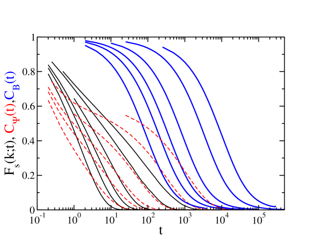
Figure 1: The self-intermediate scattering function $F_{s}(k;t)$ (solid black lines), the bond-orientational correlation $C_{\Psi}(t)$ (dashed red lines), and the bond-breaking correlation function $C_{B}(t)$ (thick blue lines) for $T=1.0,0.8,0.7,0.6,0.5$, and 0.45 listed from left to right. Results are shown for 250,000 particles systems except for $F_{s}(k;t)$ at $T=0.45$, where a 4 million particle system is needed to remove finite size effects.

Bond-orientational relaxation is quantified by the bond-angle correlation function

$$C_{\Psi}(t)=\frac{\left<\sum_{n}\Psi_{6}^{n}(t)\left[\Psi_{6}^{n}(0)\right]^{*}\right>}{\left<\sum_{n}\left|\Psi_{6}^{n}(0)\right|^{2}\right>},$$ (3)

where $\Psi_{6}^{n}(t)=(N_{b}^{n})^{-1}\sum_{m}e^{i6\theta_{nm}(t)}$ and ^∗ denotes the complex conjugate. The sum over $m$ is over the neighbors of particle $n$ determined through Voronoi tessellation and the sum over $n$ is over all particles in the system. $N_{b}^{n}$ is the number of neighbors of particle $n$, and $\theta_{nm}$ is the angle made by the bond between particle $n$ and $m$ with respect to an arbitrary axis.

To examine bond-breaking events, we first define bonded particles. To be consistent with previous work [5, 6, 8, 9], we define particles of type $\alpha$ and $\beta$ as bonded if $\left|\mathbf{r}_{n}^{\alpha}-\mathbf{r}_{m}^{\beta}\right|<1.15\sigma_{\alpha\beta}$. The bond is broken at a later time if $\left|\mathbf{r}_{n}^{\alpha}-\mathbf{r}_{m}^{\beta}\right|>1.5\sigma_{\alpha\beta}$. We define a function $Z_{n}(t)$ which is the number of broken bonds of particle $n$ at a time $t$. Therefore $Z_{n}(t=0)$ is zero and $Z_{n}(t=\infty)$ is the number of bonds particle $n$ had at $t=0$. The bond-breaking correlation function is defined as

$$C_{B}(t)=1-\frac{N^{-1}\left<\sum_{n}Z_{n}(t)\right>}{\left<N_{B}\right>},$$ (4)

where $\left<N_{B}\right>=N^{-1}\left<\sum_{n}Z_{n}(\infty)\right>$ is the average number of bonds per particle.

Shown in Fig. 1 are $F_{s}(t)$ (solid black lines), $C_{\Psi}(t)$ (dashed red lines), and $C_{B}(t)$ (thick blue lines) as a function of time for $T=1.0,0.8,0.7,0.6,$ 0.5, and 0.45 listed from left to right. As noted in previous work [3], there is no plateau in the self-intermediate scattering function if the simulated system is large enough, which is in contrast to simulations of three-dimensional glass forming systems. However, a plateau does begin to emerge in the bond-orientational correlation function $C_{\Psi}(t)$. Furthermore, it can be seen in Fig. 1 that the decay time of $C_{\Psi}(t)$ increases faster with decreasing temperature than $F_{s}(k;t)$. The characteristic decay time of $C_{B}(t)$ is longer then that of either $F_{s}(k;t)$ or $C_{\Psi}(t)$ at each temperature. While the particles are moving translationally and even the orientations of the bonds between neighboring particles relax, the particles have not lost their neighbors.

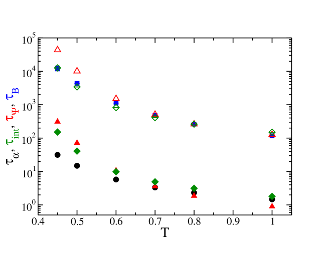
Figure 2: The alpha-relaxation time $\tau_{\alpha}$ (black circles), the integrated relaxation time $\tau_{\mathrm{int}}$ (green diamonds), the bond-orientational relaxation time $\tau_{\Psi}$ (solid red triangles), and the bond-breaking relaxation time $\tau_{B}$ (blue squares) as a function of temperature $T$. The open red triangles are the bond-orientational relaxation times scaled so that the $\tau_{\Psi}$ equals $\tau_{B}$ at $T=0.8$. The open green diamonds is the integrated relaxation time scaled so that equal $\tau_{\mathrm{int}}$ equals $\tau_{B}$ at $T=0.8$.

To quantify the decay time we define the relaxation times $\tau_{\alpha}$, $\tau_{\Psi}$, and $\tau_{B}$ through $F_{s}(k;\tau_{\alpha})=e^{-1}$, $C_{\Psi}(\tau_{\Psi})=e^{-1}$, and $C_{B}(\tau_{B})=e^{-1}$. These relaxation times are shown in Fig. 2 as a function of temperature. The relaxation time $\tau_{\alpha}$ grows the slowest with decreasing temperature. The bond-breaking relaxation times $\tau_{B}$ is larger than the other two relaxation times over this temperature range. However, $\tau_{\Psi}$ grows faster with decreasing temperature than either $\tau_{\alpha}$ or $\tau_{B}$. To demonstrate this faster growth, we show as open red triangles $a\tau_{\Psi}$ where $a$ is the ratio $\tau_{B}/\tau_{\Psi}$ at $T=0.8$.

We note that we defined $\tau_{\alpha}$ in the standard way, but this definition is not the only way to determine a relaxation time. Another method would be to examine an integrated relaxation time $\tau_{\mathrm{int}}=\int_{0}^{\infty}F_{s}(k;t)dt$, which would be equal to $\tau_{\alpha}$ as defined above if $F_{s}(k;t)$ decayed exponentially and proportional to $\tau_{\alpha}$ if time-temperature superposition holds. However, time-temperature superposition does not hold for $F_{s}(k;t)$ for the two-dimensional glass former, so we also examined $\tau_{\mathrm{int}}$, which is shown as filled green diamonds in Fig. 2.

We find that $\tau_{\mathrm{int}}$ grows with decreasing temperature at the same rate as $\tau_{B}$, which we demonstrate by multiplying $\tau_{\mathrm{int}}$ by a constant $b$ such that $b\tau_{\mathrm{int}}$ is equal to $\tau_{B}$ at $T=0.8$, and this scaling is shown as the open green triangles in Fig. 2.

We note that time-temperature superposition holds very well for $C_{B}(t)$, and it also holds for the final decay of $C_{\Psi}(t)$, i.e. for $C_{\Psi}(t)\leq 0.2$, see Fig. 3. We checked whether our results for the temperature dependence of the bond orientational relaxation time depend on our definition of $\tau_{\Psi}$. If we define a relaxation time $\tau_{\Psi}^{c}$ through $C_{\Psi}(\tau_{\Psi}^{c})=c$ with $c\leq e^{-1}$, the choice of $c$ does not alter our conclusions. Specifically, $\tau_{\Psi}^{c}$ with $c\leq e^{-1}$ increases faster with decreasing temperature than $\tau_{\alpha}$, $\tau_{\mathrm{int}}$, and $\tau_{B}$.

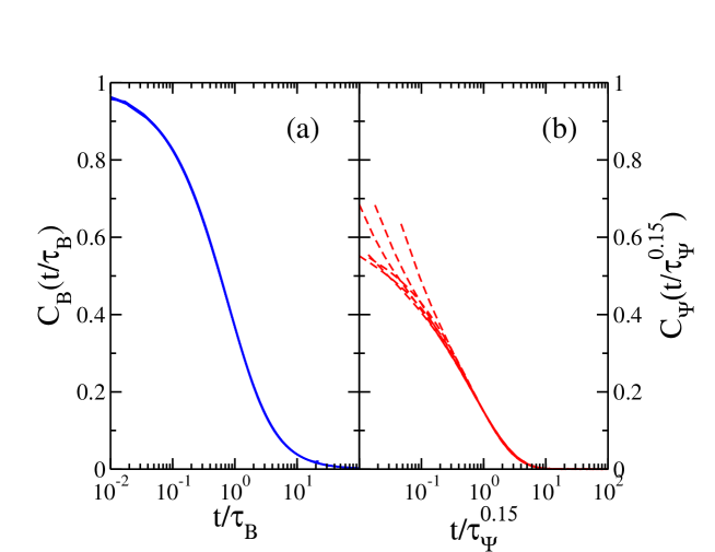
Figure 3: (a) The bond-breaking correlation function $C_{B}(t)$ where the time axis is rescaled by $\tau_{B}$. (b) The bond-orientational relaxation function $C_{\Psi}(t)$ where the time axis is rescaled by $\tau_{\Psi}^{0.15}$ where $\tau_{\Psi}^{0.15}$ is defined through $C_{\Psi}(\tau_{\Psi}^{0.15})=0.15$. Time-temperature superposition holds very well for the whole time dependence of $C_{B}(t)$ and for the final decay of $C_{\Psi}(t)$. In both (a) and (b) $T=1.0$, 0.8, 0.7, 0.6, 0.5, and 0.45 are shown.

Finally, a visual inspection of the bond-breaking and bond-orientational correlation functions suggests that the bond-breaking relaxation is less stretched that the bond-orientational one. To quantify the temperature dependence of the shape of these correlation functions we fit $C_{B}(t)$ and $C_{\Psi}(t)$ to a stretched exponential $A\exp(-(t/\tau)^{\beta})$. We found that the the stretching exponent $\beta$ was independent of temperature for $C_{B}(t)$, and was $0.673\pm 0.004$. The stretching exponent for $C_{\Psi}(t)$ was $\beta=0.651\pm 0.006$ at $T=1.0$ and $\beta\approx 0.62\pm 0.01$ for $0.45\leq T\leq 0.8$.

4 Dynamic Correlation Lengths

It has been suggested that the characteristic size of clusters of correlated relaxation events can define a dynamic correlation length that accompanies the glass transition. Here we examine correlations between bond-breaking events and correlations of bond-orientational relaxation. To find the dynamic correlation length it has become standard practice to define a four-point structure factor

$$S_{4}^{w}(q;t)=\frac{1}{N}\left<\sum_{nm}w_{n}(t)w_{m}^{*}(t)e^{i\mathbf{q}\cdot[\mathbf{r}_{n}(0)-\mathbf{r}_{m}(0)]}\right>,$$ (5)

and determine a characteristic size of mobile or immobile clusters from the small $q$ behavior of $S_{4}^{w}(q;t)$ [1]. Importantly, the four point structure factor involves a time dependent weight function $w_{n}(t)$ that is sensitive to the microscopic dynamic events associated with particle $n$. Thus, the weight function determines the dynamic events whose spatial correlations the four-point structure factor measures.

In previous work we examined the characteristic size of clusters of slow particles [3]. To this end we used a weight function that selects slow particles, which we defined as particles that moved less than $a=0.22$, $\Theta(a-|\mathbf{r}_{n}(t)-\mathbf{r}_{n}(0)|)$ where $\Theta$ is Heaviside’s step function. We found that the characteristic size of clusters of particles which are slow on the time scale of the $\alpha$ relaxation time, $\tau_{\alpha}$, grows linearly with $\tau_{\alpha}$ for two-dimensional systems evolving with Newtonian dynamics [3]. This was in contrast with the $\ln(\tau_{\alpha})$ growth that was observed for fragile glass formers in three dimensions [12, 16]. Here we examine correlations of bond-breaking events. To this end we use $Z_{n}(t)$ as the weight function $w_{n}(t)$. We also study correlated bond-orientational relaxation by using $\Psi_{6}^{n}(t)[\Psi_{6}^{n}(0)]^{*}$ as the weight function. To determine the dynamic correlation length $\xi_{w}(t)$ we fit $S_{4}^{w}(q;t)$ to an Ornstein-Zernicke form, $S_{4}^{w}(0;t)/[1+(q\xi_{w}(t))^{2}]$, for small $q$. We denote dynamic correlation lengths characterizing the spatial correlations of bond-breaking events as $\xi_{B}(t)$ and dynamic correlation lengths measuring the spatial correlations of bond-orientational relaxation as $\xi_{\Psi}(t)$. For a comparison, we also present the dynamic correlation lengths characterizing the size of clusters of slow particles, which are denoted as $\xi_{O}(t)$.

We begin by examining the time-dependence of the correlation lengths $\xi_{B}(t)$ and $\xi_{\Psi}(t)$. Shown in Fig. 4 are the dynamics correlation lengths $\xi_{B}(t)$ and $\xi_{\Psi}(t)$ as a function of time for $T=1.0,0.8,0.7,0.6,$ 0.5, and 0.45. For short times, $\xi_{B}(t)$ (squares) and $\xi_{\Psi}(t)$ (circles) are equal and grow approximately as $\ln(t)$ (solid line). We note that the $\ln(t)$ growth of the correlation length is similar to what was reported for mobility correlations in a three-dimensional hard sphere system [16], and is consistent with the growth of mobility correlations for several fragile glass formers [12]. We found that the growth of $\xi_{\Psi}(t)$ is arrested before that of $\xi_{B}(t)$. Both $\xi_{\Psi}(t)$ and $\xi_{B}(t)$ peak at their specific characteristic times and then decrease for later times. We recall that in a three-dimensional hard sphere system, there was a plateau in the overlap length and no peak was observed [16], but a peak in the overlap length was reported in the three-dimensional Kob-Andersen system [9]. While it is difficult to determine the precise location of the peak, $\xi_{\Psi}(t)$ peaks at a time approximately five times larger than $\tau_{\Psi}$ and $\xi_{B}(t)$ peaks at a time that is about 2.5 times smaller than $\tau_{B}$.

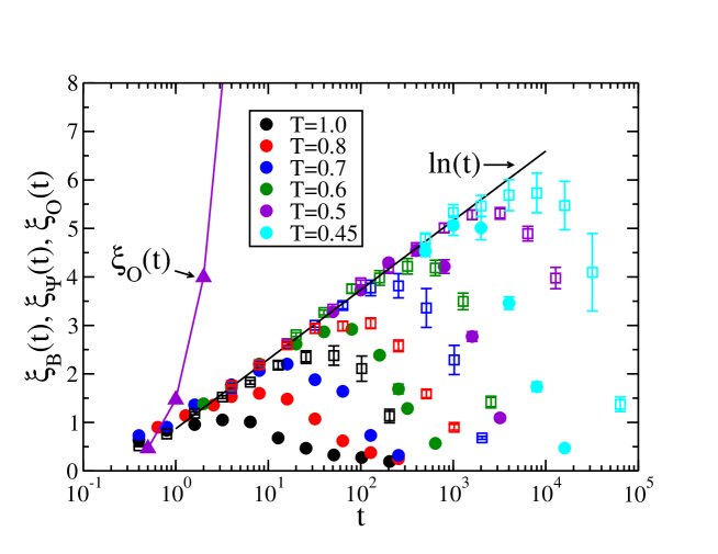
Figure 4: The time dependence of the bond-orientational correlation length $\xi_{\Psi}$ (solid circles) and the bond-breaking correlation length $\xi_{B}$ (open squares) for $T=1.0,0.8,0.7,0.6,$ and 0.5. Initially, the two correlation lengths are approximately equal, but $\xi_{\Psi}$ stops growing at an earlier time than $\xi_{B}$. Both length scales have a period of logarithmic growth (solid line) for $T\leq 0.7$, before a peak and a decrease at later times. The triangles is the time dependence of the overlap length calculated for $T=0.5$.

Shown as the triangles in Fig. 4 is the overlap length, i.e. the length characterizing mobility correlations, $\xi_{O}(t)$, for $T=0.5$. At short times, it grows approximately linearly with time. This initial linear growth of $\xi_{O}(t)$ occurs for all temperatures (not shown for clarity). Similar to the universal growth of $\xi_{\Psi}(t)$ and $\xi_{B}(t)$, the time dependence of $\xi_{O}(t)$ is the same for each temperature at shorter times and there are deviations from the master curve at later times. Importantly, Fig. 4 demonstrates the much stronger growth of the overlap length than the lengths characterizing spatial correlations of bond-breaking events and bond-orientational relaxation.

To compare the two lengths characterizing spatial correlations of bond-breaking events and bond-orientational relaxation, we show the temperature dependence of their maximum values in Fig. 5(a). Both lengths grow with decreasing temperature, but $\xi_{\Psi}^{\mathrm{max}}$ (red circles) grows faster than $\xi_{B}^{\mathrm{max}}$ (blue squares). In Fig. 5(a) we show the ratio of the two lengths, $\xi_{B}^{\mathrm{max}}/\xi_{\Psi}^{\mathrm{max}}$. We note that the faster growth of $\xi_{\Psi}^{\mathrm{max}}$ is consistent with $\xi_{\Psi}^{\mathrm{max}}$ occurring at a multiple of $\tau_{\Psi}$, with $\tau_{\Psi}$ growing faster with decreasing temperature than $\tau_{B}$.

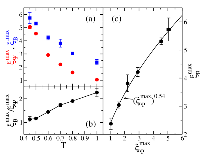
Figure 5: (a) The temperature dependence of $\xi_{B}^{\mathrm{max}}$ and $\xi_{\Psi}^{\mathrm{max}}$. (b) The ratio $\xi_{B}^{\mathrm{max}}/\xi_{\Psi}^{\mathrm{max}}$ of the maximum of the correlation lengths $\xi_{B}(t)$ and $\xi_{\Psi}(t)$ as a function of temperature. (c) The correlation length $\xi_{B}^{\mathrm{max}}$ versus the correlation $\xi_{\Psi}^{\mathrm{max}}$. The line shows a fit to the function $\xi_{B}^{\mathrm{max}}=a(\xi_{\Psi}^{\mathrm{max}})^{\gamma}$ with $\gamma=0.54\pm 0.05$.

We note an approximate power-law relationship between the two lengths: a fit of $\xi_{B}^{\mathrm{max}}$ to $a(\xi_{\Psi}^{\mathrm{max}})^{\gamma}$ resulting in $\gamma=0.54\pm 0.05$ represents the data within error, see Fig. 5(c). However, a larger range of correlation lengths would be needed to confirm this relationship. In particular, it would be interesting to investigate what happens at lower temperatures.

5 Dynamic Susceptibilities

The ensemble independent susceptibility $S_{4}^{w}(0;t)=\lim_{q\rightarrow 0}S_{4}^{w}(q;t)$ is a measure of the strength of the dynamic heterogeneity probed by the weight function $w(t)$. However, it can be difficult to calculate $S_{4}^{w}(0;t)$ since one has to either simulate large systems [13] or account for suppressed global fluctuations of the simulational ensemble [14, 15, 16]. Typically, the ensemble dependent susceptibilities are studied and the behavior of the full dynamic susceptibility $S_{4}^{w}(0;t)$ and the dynamic correlation length $\xi_{w}(t)$ is inferred. Here we will examine the ensemble dependent susceptibilities $\chi_{4}^{w}(t)$ and examine how they are related to the ensemble independent susceptibilities and the dynamic correlation lengths.

The ensemble dependent dynamic susceptibilities are given by

$$\chi_{4}^{w}(t)=\frac{1}{N}\left<\left|\sum_{n}w_{n}(t)\right|^{2}\right>-\left<\sum_{n}w_{n}(t)\right>^{2},$$ (6)

where $\left<\cdot\right>$ denotes an average in the $NVT$ ensemble. The ensemble independent susceptibilities $S_{4}^{w}(0;t)=\lim_{q\rightarrow 0}S_{4}^{w}(q;t)$ are obtained from the fits to $S_{4}^{w}(q;t)$.

Shown in Fig. 6 are $\chi_{4}^{\Psi}(t)$ (lower red lines) and $\chi_{4}^{B}(t)$ (upper blue lines) on a log-log scale for $T=1.0,0.8,0.7,0.6,0.5,$ and 0.45. The bond-orientational susceptibility $\chi_{4}^{\Psi}(t)$ grows as $\sqrt{t}$, Fig. 7, before it plateaus and then decays to a constant. However the bond-breaking susceptibility $\chi_{4}^{B}(t)$ grows linearly with time, Fig. 7, before the peak. For a given temperature, $\chi_{4}^{B}(t)$ peaks at a later time than $\chi_{4}^{\Psi}(t)$.

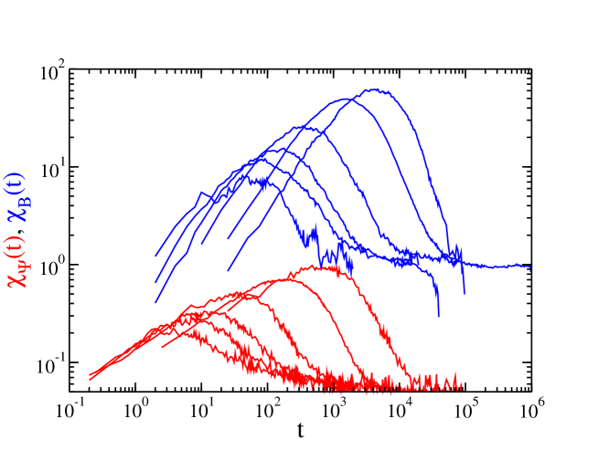
Figure 6: The ensemble dependent susceptibilities $\chi_{4}^{\Psi}(t)$ (lower red lines) and $\chi_{4}^{B}(t)$ (upper blue lines) for $T=1.0,0.8,0.7,0.6,0.5,$ and 0.45 listed from left to right.

We compare the ensemble dependent susceptibility $\chi_{4}^{w}(t)$ to the ensemble independent susceptibility $S_{4}^{w}(0;t)$ in Fig. 7. We find that $S_{4}^{B}(0;t)$ is larger than $\chi_{4}^{B}(t)$, but its peak is at around the same time as that of $\chi_{4}^{B}(t)$. Note that the ensemble independent susceptibility is expected to be equal to or larger than the ensemble dependent susceptibility [14]. Surprisingly, we find that $S_{4}^{\Psi}(0;t)$ is equal to $\chi_{4}^{\Psi}(t)$ within error for $T=0.5$ over the time range we studied. We note that for higher temperatures we found that $S_{4}^{\Psi}(0,t)$ is slightly larger than $\chi_{4}^{\Psi}(t)$ in general.

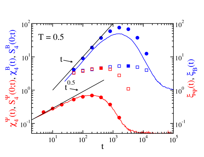
Figure 7: The ensemble dependent susceptibilities $\chi_{4}^{\Psi}(t)$ (lower red line) and $\chi_{4}^{B}(t)$ (upper blue line) compared to the ensemble independent susceptibility $S_{4}^{\Psi}(0;t)$ (lower red circles) and $S_{4}^{B}(0;t)$ (upper blue circles) for $T=0.5$. Note that $\chi_{4}^{\Psi}(t)$ is equal to $S_{4}^{\Psi}(0;t)$ to within error for this temperature. The squares are the correlation lengths $\xi_{\Psi}(t)$ (red) and $\xi_{B}(t)$ (blue), where the filled square is the maximum length. The maximum length occurs at a time slightly larger than the time of the susceptibility peak.

We also show the time dependence of the correlation lengths $\xi_{B}(t)$ (blue squares) and $\xi_{\Psi}(t)$ (red squares) for $T=0.5$ in Fig. 7. As noted in Sec. 4, $\xi_{B}(t)$ and $\xi_{\Psi}(t)$ are initially equal, but $\xi_{\Psi}(t)$ plateaus and decreases before $\xi_{B}(t)$. Note that the maximum length, denoted as filled squares, occurs slightly after the peak in $\chi_{B}(t)$ and $\chi_{\Psi}(t)$ for both correlation lengths. Recall that $\tau_{B}$ is larger than the time of the maximum of $\xi_{B}(t)$ and $\tau_{\Psi}$ is smaller than the time of the maximum of $\xi_{\Psi}(t)$. Therefore, it seems appropriate to compare the correlation lengths around the maximum of the susceptibility, which is around the maximum lengths for $\xi_{B}(t)$ and $\xi_{\Psi}(t)$. In fact, such a procedure was used in Ref. [9].

6 Conclusions

We examined bond-orientational relaxation and bond-breaking events in a model two-dimensional glass forming system. We found that the characteristic time for particles to lose their neighbors, the bond-breaking relaxation time, is longer than the decay time of bond-orientational correlations and the decay time of the self-intermediate scattering function. However, the bond-orientational correlation time increases faster with decreasing temperature than the bond-breaking relaxation time over the temperature range studied.

We also examined the spatial correlations of bond-orientational relaxation and bond-breaking events. We found that at each temperature the characteristic size of correlated domains of bond-orientational relaxation and bond-breaking events were equal at short times, but the characteristic size of domains of correlated bond-orientational relaxation saturates at an earlier time than for bond-breaking events and the associated maximum correlation length is smaller. However, the maximum correlation length for bond-orientational relaxation grows faster with decreasing temperature than the maximum correlation length for bond-breaking events. The correlation lengths appear to be related by a power law where $\xi_{B}^{\mathrm{max}}\propto(\xi_{\Psi}^{\mathrm{max}})^{\gamma}$ with $\gamma\approx 0.54$, but a larger range of length scales would needed to verify this relationship.

While we did not verify that the correlations of bond-orientational relaxation grow as mobility correlations in three dimensions, this result would be expected since bond-orientational relaxation time grows as structural relaxation time in three dimensions. It has already been demonstrated that bond-breaking correlation length grows as mobility correlation length in three-dimensions, but bond-breaking correlation length grows slower than mobility correlation length in two dimensions [9]. However, in two dimensions there are now three time dependent correlation lengths with different temperature dependence. We note that the bond-orientational and the bond-breaking correlation lengths appear to be related, and future studies of lower temperature two-dimensional systems needs to be performed to understand this relationship fuller.

We found that the ensemble dependent susceptibility calculated in an NVT ensemble and the ensemble independent susceptibility each has a peak at a time slightly less than the time of the maximum of the bond-orientational and the bond-breaking correlation lengths. Importantly, the ensemble independent and the ensemble dependent susceptibilities peak at the same time. Note that the peak time of the bond-orientational dynamic susceptibility is larger than the bond-orientational relaxation time, but the peak time of the bond-breaking dynamic susceptibility is at a time smaller than the bond-breaking relaxation time. Therefore, the dynamic correlation length calculated at the bond-orientational relaxation time is still growing, but the dynamic correlation length calculated at the bond-breaking relaxation time has already reached its peak and is decreasing.

Appendix A Calculating Dynamic Correlation Lengths

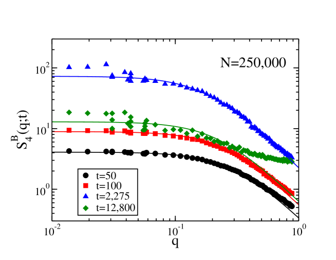
Figure 8: Some example four-point structure factors $S_{4}^{B}(q;t)$ for $T=0.5$. For $q\approx 0.3$ and $q\approx 0.04$ several wave-vectors with the same magnitude but are calculated with $q$ in different directions are shown. The lines are Ornstein-Zernicke fits. The range of $q$ values are chosen such that the Ornstein-Zernicke fits give a correlation length that is consistent with analyzing $G_{4}^{B}(r;t)$.

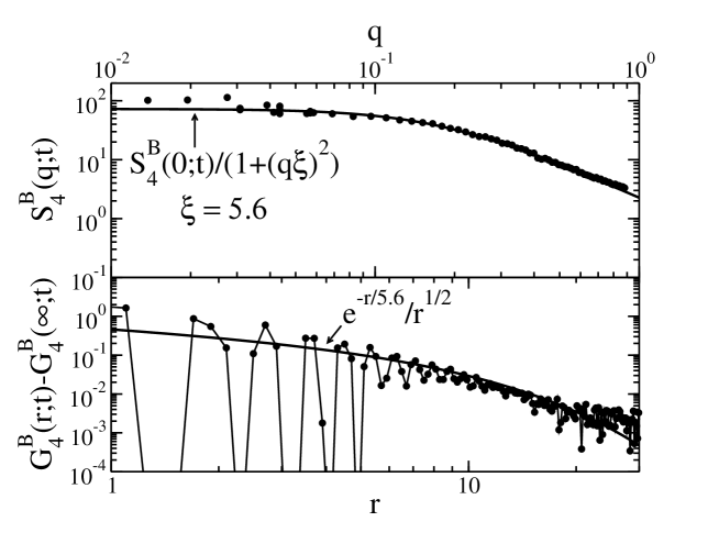
Figure 9: The upper figure shows the four-point structure factor $S_{4}^{B}(q;t)$ and the Ornstein-Zernicke fit to obtain the correlation length at $t=2,275$, which is close to time of the peak of the dynamic susceptibility $\chi_{4}^{B}(t)$. The lower figure is the associated four-point correlation function $G_{4}^{B}(r;t)-G_{4}^{B}(\infty;t)$ and the verification that the length from the Ornstein-Zernicke fit is compatible with the decay of $G_{4}^{B}(r;t)$.

In this appendix we outline the procedure we use to obtain dynamic correlation lengths in our study. We found that it was difficult to determine how to fit the small wave-vector behavior of $S_{4}^{w}(q;t)$ from the four-point structure factor alone at times later than the peak of the dynamic susceptibility due to noise for small wave-vectors.

Shown in Fig. 8 is $S_{4}^{B}(q;t)$ at T=0.5 for several times. For short times, the small $q$ values converge and the Ornstein-Zernicke function provided good fits to $S_{4}^{B}(q;t)$. Several fits are shown in the figure. At later times, there is significant noise in the small $q$ values of $S_{4}^{B}(q;t)$ and fits over different ranges of $q$ resulted in a large range of correlation lengths. To determine the correct correlation length, we also calculated the four-point pair correlation function

$$G_{4}^{w}(r;t)=\frac{V}{N^{2}}\left<\sum_{n}\sum_{m\neq n}w_{n}(t)w_{m}^{*}(t)\delta(\mathbf{r}-\mathbf{r}_{nm}(0))\right>,$$ (7)

where $\mathbf{r}_{nm}(0)=\mathbf{r}_{n}(0)-\mathbf{r}_{m}(0)$. We checked that the large $r$ decay of $G_{4}^{w}(r;t)$ was consistent with the Ornstein-Zernicke fit. To this end we found $G_{4}^{w}(r;t)$ for large $r$ by fitting $G_{4}^{w}(r;t)$ for $r>100$ to a constant $G_{4}^{w}(\infty,t)$. We then examined $G_{4}^{w}(r;t)-G_{4}^{w}(\infty,t)$ and verified that it was consistent with the Ornstein-Zernicke fit by verifying that the decay followed $e^{-r/\xi}/\sqrt{r}$. This functional form is obtained from noting that the inverse Fourier Transform in two dimensions of $1/[1+(q\xi)^{2}]$ is proportional to $K_{0}(r/\xi)$ where $K_{0}$ is the modified Bessel function of the second kind, and that $K_{0}(r/\xi)$ is well approximated by $e^{-r/\xi}/\sqrt{r}$ for large $r$. We show an example of this verification for $T=0.5$ and $t=2\,275$ in Fig. 9. To calculate $G_{4}^{B}(r;t)$ for large systems we used the technique introduced by Bernard and Krauth [17].

References

References

- [1] Berthier L, Biroli G, Bouchaud J-P, Cipelletti L, and Van Saarloos W 2011 Dynamic Heterogeneities in Glasses, Colloids and Granular Media Oxford University Press, Oxford.
- [2] Widmer-Cooper A, Harrowell P and Fynewever H 2004 Phys. Rev. Lett. 93 135701.
- [3] Flenner E and Szamel G 2015 Nature Commun. 6 7392.
- [4] Strandburg K J 1988 Rev. Mod. Phys. 60 161.
- [5] Yamamoto R and Onuki A 1998 Phys. Rev. E 58 3515.
- [6] Yamamoto R and Onuki A 2000 J. Phys.: Condens. Matter 12 6323.
- [7] Flenner E and Szamel G 2015 J. Phys. Chem. B 119 9188.
- [8] Shiba H, Kawasaki T and Onuki A 2012 Phys. Rev. E 86 041504.
- [9] Shiba H, Kawasaki T and Kim K arXiv:1510.02546v1.
- [10] Hocky G M and Reichman D R 2013 J. Chem. Phys. 138 12A537.
- [11] Andersen J A, Lorenze C D and Travesse A 2008 J. Comput. Phys. 227 5342; https://codeblue.umich.edu/hoomd-blue/.
- [12] Flenner E, Staley H and Szamel G 2014 Phys. Rev. Lett. 112 097801.
- [13] Karmakar S, Dasgupta C and Sastry S 2010 Phys. Rev. Lett. 105 015701.
- [14] Berthier L, Biroli G, Bouchaud J-P, Cipelletti L, El Masri D, L’Hôte D, Ladieu Fand Pierno M, 2005 Science 310, 1797.
- [15] Flenner E and Szamel G 2010 Phys. Rev. Lett. 105 217801.
- [16] Flenner E, Zhang M and Szamel G 2011 Phys. Rev. E 83 051501.
- [17] Bernard E P and Krauth W 2011 Phys. Rev. Lett. 107 155704.