Hong Kong - Shanghai Connect / Hong Kong - Beijing Disconnect (?):

Scaling the Great Wall of Chinese Securities Trading Costs

Ravi Kashyap

SolBridge International School of Business / City University of Hong Kong

Hong Kong; Shanghai; Connect; Trading Cost; Market Impact; Uncertainty

JEL Codes: G15 International Financial Markets; D53 Financial Markets; G17 Financial Forecasting and Simulation; F37 - International Finance Forecasting and Simulation

1 Abstract

We utilize a fundamentally different model of trading costs to look at the effect of the opening of the Hong Kong Shanghai Connect that links the stock exchanges in the two cities, arguably the biggest event in international business and finance since Christopher Columbus set sail for India. We design a novel methodology that compensates for the lack of data on trading costs in China. We estimate trading costs across similar positions on the dual listed set of securities in Hong Kong and China, hoping to provide useful pieces of information to help scale “The Great Wall of Chinese Securities Trading Costs”. We then compare actual and estimated trading costs on a sample of real orders across the Hong Kong securities in the dual listed pair to establish the accuracy of our measurements.

The primary question we seek to address is “Which market would be better to trade to gain exposure to the same (or similar) set of securities or sectors?” We find that trading costs on Shanghai, which might have been lower than Hong Kong, might have become higher leading up to the Connect. What remains to be seen is whether this increase in trading costs is a temporary equilibrium due to the frenzy to gain exposure to Chinese securities or whether this phenomenon will persist once the two markets start becoming more and more tightly coupled.

It would be interesting to see if this pioneering policy will lead to securities exchanges across the globe linking up one another, creating a trade anything, anywhere and anytime marketplace. Looking beyond mere trading costs, such studies can be used to gather some evidence on what effect the mode of governance and other aspects of life in one country have on another country, once they start joining up their financial markets.

2 Introduction

On November 17, 2014, amidst the backdrop of the protests in Hong Kong regarding electoral reform, the plan to connect the stock markets of Hong Kong and Shanghai proceeded after a slight delay over the preceding weeks. The opening of the Hong Kong - Shanghai connect, henceforth “ Connect”, opens a new era in the cross border flow of capital into and out of China. While the proximate intention behind this scheme could be to increase the trading of securities and bolster the equity markets in China, the fundamental reasoning could be to liberalize the financial system and spur economic growth, which has fallen sharply from the double digit rates of the recent past (End-note 2). Whether this is part of a bigger scheme to financially join the two economies and aid greater political unification is a matter to be studied over the next few decades. Also of interest would be to see if this pioneering policy will lead to securities exchanges across the globe linking up one another, creating a trade anything, anywhere and anytime financial marketplace.

2.1 Stock Markets and Economic Growth

There is a vast body of literature regarding financial liberalization and economic growth. Bekaert, Harvey and Lundblad (2005) show that equity market liberalizations on average lead to an increase in annual real economic growth rates. They point out that equity market liberalization directly reduces financing constraints by making available more foreign capital, and foreign investors may insist on better corporate governance, which should promote financial development. Levine (2001) suggests that stock markets influence growth through efficient capital allocation. New information can lead to profitable trading and improved information about firms improves resource allocation and hence economic growth.

Levine and Zervos (1996, 1998a) find that stock market liquidity – as measured both by the value of stock trading relative to the size of the market and by the value of trading relative to the size of the economy – is positively and significantly correlated with current and future rates of economic growth, capital accumulation and productivity growth. Levine and Zervos (1998b) looks at the stock market liquidity following capital control liberalization in 15 emerging market economies and find that stock markets tend to become larger, more liquid, more volatile and more integrated following liberalization. Building on the consensus that stock market liberalizations can reduce the cost of equity capital, Henry (2000), finds that there can be a boom in private investments following the liberalization. Beck and Levine (2004) show that stock markets are important for economic growth independent of the banking sector, with some evidence that the two could provide different set of financial services and could be complimentary to one other. Deeg and O‘Sullivan (2009) chronicle the shift from predominantly state controlled financial systems to multilateral agencies like the International Monetary Fund. They emphasize the increasing significance of regulatory regimes generated through the interactions of public and private actors that extend across national boundaries. The discussion turns towards the consequences of the current trends toward financialization and the recovery that is currently underway after the 2008 collapse. Epstein (2005) defines financialization, broadly, as the increasing role of financial motives, financial markets, financial actors and financial institutions in the operation of the domestic and international economies; and goes on to a deeper discussion regarding the dimensions of financialization, its implications for economic stability, growth, income distribution, political power, policy formulation. Adding to the importance of liquidity for asset pricing, Bekaert, Harvey and Lundblad (2007) use measures of liquidity constructed using daily returns and the length of the non-trading interval to show that liquidity predicts future returns. While admitting that transaction data are hard to obtain in emerging markets, they justify the usage of this alternate measure for emerging markets.

One aspect that stands out among all these studies is that none of them explicitly consider the implicit trading costs or the uncertainty associated with market prices, either in the measures of liquidity or otherwise, while the actual transfer of capital happens through the means of trading in the stock markets. In this study, we focus heavily on the trading cost element when there is a major liberalization event. We utilize a fundamentally different method of measuring trading costs and apply it to study one of the, if not the, biggest event in international business and finance since Christopher Columbus set sail for India. If we find that trading costs are being influenced heavily by market liberalizations, the lessons from such a study can be manifold, change in transaction costs could be a signal of potential building up of a bubble and a later bust. When not indicative of such extreme situations, trading or transaction costs, could serve to highlight whether the transfer of capital or investment is happening as expected and whether foreign investors view on liquidity has been shaped positively, to bring in additional sources of capital.

2.2 The Connect

The official announcement of the “Connect” program launch on April 10, 2014, sent financial intermediaries into an arms race, of sorts, to be prepared to trade on the connect right from the first day of the program. Before the Connect, shares listed in China, called A-shares, were only available to foreign institutional investors through certain investment products called Qualified Foreign Institutional Investor (QFII) funds and other such investment vehicles. Likewise, formal channels of overseas investment by Chinese residents to the Qualified Domestic Institutional Investor (QDII) schemes. The Connect program allows a small number of securities listed on the Shanghai Stock Exchange (SSE) to be traded by participants in Hong Kong and vice versa. Under this pilot program, shares eligible to be traded through the Northbound Trading Link (from Hong Kong to Shanghai) will comprise all the constituents of the SSE 180 Index and SSE 380 Index, and shares of all SSE-listed companies which have issued both A shares and H shares. Shares eligible to be traded through the Southbound Trading Link (from Shanghai to Hong Kong) comprise all the constituents of the Hang Seng Composite Large Cap Index and Hang Seng Composite Mid Cap Index, and shares of all companies listed on both SSE and Stock Exchange of Hong Kong (SEHK). The initial expected date of the launch was towards the middle of October. The delay also gives us a chance to study the reaction of market participants on the announcement of the delay and the trends in the run up to the final launch.

2.3 Some Other Tidbits

• Launched at 9:30 AM November 17, 2014. In the first seven minutes (Figure 1), more than 50% of the Quota was used up (End-note 3).

Figure 1: First Seven Minutes of Trading

• HK Exchange Total Market Cap $3.1 trillion (Currently 6th globally), Shanghai Exchange Total Market Cap $2.4 trillion (7th) - Combined Market Cap will put them in the top three.

• Currently QFII Quota (Includes other asset classes as well) around US $150 Billion. This is available only to large institutions

• 568 Securities in the Northbound (Hong Kong to Shanghai), 268 in the Southbound (Shanghai to Hong Kong), 68 Dual Listed Securities

• Daily Northbound Quota is RMB 13 Billion (Around $2 Billion USD), Daily Southbound Quota is RMB 10.5 Billion (Less than $2 Billion USD)

• Market Cap (Approximate) on Hong Kong Connect Securities - $105 Billion USD

• Daily Average Daily Volume, ADV, (Approximate) on Hong Kong Connect Securities - $ 5 Billion USD

• Market Cap (Approximate) on Shanghai Connect Securities - $53 Billion USD

• Daily ADV (Approximate) on Shanghai Connect Securities - $30 Billion USD

2.4 Dual Listing Dynamics

There is again a massive amount of literature on dual listing and its effect on stock returns. Serra (1999) investigates the effects on stock returns of dual-listing on an international exchange across a sample of emerging market securities. The results from the sample they analyze confirm previous empirical findings that there are positive abnormal returns before listing and a significant decline in expected returns following the listing. Such a result is explained by the extent of integration of capital markets, where integration is defined as a situation where investors earn the same risk-adjusted expected return on similar financial instruments in different markets. In a fully integrated market, the price of risk would be the same in all markets and this would be the compensation for the systemic risk factors that occur globally. Where the extent of integration is less or where there is segmentation, risk associated with local factors is priced into the security returns, yielding different rewards to risk. Dual listing or other forms of cross listing would mitigate segmentation by improving risk sharing. The increased liquidity and investor awareness might lower the required rate of return. Cross listing could also reduce the cost of capital, acting as an incentive for firms.

Shleifer and Vishny (1997) in their seminal work on the limits of arbitrage point out that risk free arbitrage rarely exists in the real world. Most arbitrageurs, who are specialized investors, managing assets on behalf of others, face the possibility of interim liquidations before the price disparity is restored, sometimes even when the arbitrage opportunity is at its best, due to the short term losses that can crop up from the diverging prices. This limitation on the capital available for arbitrage could even amplify the arbitrage opportunity by forcing the actions of investors against the direction of trading that could potentially restore the price deviation and is compounded due to any long run fundamental risk faced by the arbitrageurs. Gromb and Vayanos (2010) emphasize costs that arbitrageurs could face, like a) risk, both fundamental and non-fundamental; b) cost of short selling; c) leverage and margin constraints; d) and constraints on equity capital. Fundamental risk arises due to asset payoffs and non-fundamental risk could be due to demand shocks generated by the set of investors who are not solely looking to profit from the arbitrage opportunity, also labeled “noise traders”.

De Jong, Rosenthal and Van Dijk (2003, 2009) continue along this line of inquiry by looking at price deviations across securities formed as a result of mergers, in which both companies remain incorporated independently. In contrast to securities listed on different exchanges by the same company, the securities could be listed on the same exchange in this case. To ensure there is no confusion in the terminology, we refer to these as Siamese twins, as opposed to the listing of shares in Hong Kong and China, which we refer to as dual listed. They show that abnormal returns could persist even after accounting for systematic risk, transaction costs and margin requirements. Market frictions are controlled for by taking into account estimates of brokerage commissions, bid-ask spreads, short rebates and capital requirements. The cost of setting up an arbitrage position is taken as half of the bid-ask spread, which lends some realism to the analysis yet remains questionable of the real costs execution traders face while implementing portfolios of large orders. Arbitrage activity could be further impeded due to the volatility of returns from arbitrage and the high incidence of negative returns, due to the uncertainty about the horizon at which prices will converge and deviations from parity. Bedi, Richards and Tennant (2003) highlight an interesting nuance that the pricing of Siamese twins converges following the announcement of unification via a raise in the price of the twin trading at a discount, while confirming that a price divergence continues to exist for regular listings on merged companies.

Peng, Miao, and Chow (2008) argue that the extent of segmentation between Hong Kong and China is high due to the restrictions imposed on the mobility of capital. An interesting point to note is that almost all dual listed companies have issued more H shares than A shares. The relatively small supply of A shares could exacerbate the price differential leading to the A share premium. Their investigation of the price dynamics reveals that the A and H price differential is stationary with a trend towards relative price convergence, where the differential will not diverge persistently from a certain level, as opposed to absolute price convergence or long term equalization, where the price gap has a long term mean of zero. In addition to micro factors, Fong, Wong and Yong (2008) consider macroeconomic factors and find that Chinese currency appreciation expectations and monetary expansion contributed to the A-H share price disparity by affecting the prices of A shares, but their influence on the prices of H shares was insignificant.

2.4.1 Main Difference from Dual Listing

• Comparing the Connect situation to a dual listed security, one main difference would be the daily and aggregate quota limits on the amount of securities, being bought and sold, that are part of this pilot connect program.

• The other difference being that participants wishing to buy shares in Shanghai need to go through their representatives or broker firms in Hong Kong and vice versa.

2.5 Unintended Consequences

Any attempt at regulatory change is best exemplified by the story of Sergey Bubka (End-note 4), the Russian pole vault jumper, who broke the world record 35 times. Attempts at regulatory change can be compared to taking the bar higher. In this case, the intended effect of the change is to provide investors’ greater access to China markets without creating price distortions and/or opportunities for abnormal profits. Despite all the uncertainty (See Kashyap 2014a, 2014b), we can be certain of one thing, that the market participants will find some way over the intended consequences, prompting another round of rule revisions, or raising the bar, if you will. (Kashyap 2015b) looks at a recent empirical example related to trading costs where unintended consequences set in. Below we mention the unknowns (or unintended consequences) that we know about (or can anticipate). What about the unknowns that we don’t know about (or cannot even imagine). The only thing, we know about these unknown unknowns are that, there must be a lot of them, hence the need for us to be eternally vigilant, compelling all attempts at risk management to make sure that the unexpected, even if it does happen, is contained in the harm it can cause, while being cognizant that this is easier said than done; a topic best saved for another time.

2.5.1 Uncertainty due to the Limited Quota

• Whenever there are limits imposed on the total amount of any good and there is no explicit mechanism to distribute it, it can lead to stock piling (in this case literally) and later distribution at a profit. It remains to be seen, if the daily quota allowed in this case is big enough to meet the demand or whether it would lead to someone accumulating shares and parceling it out later.

• Imagine just one keg of beer, a few dozen college kids and no rules as to how much beer each one gets!!!

• The imposed quota might exacerbate the possibility of arbitrage between the connect shares across the two markets.

• Due to the quota there is some execution risk, which means if the quota is filled just before an execution, the execution could get rejected. This can happen despite the fact that the SEHK plans to disseminate remaining quota balances every five seconds.

2.6 A Recipe for the Skeptics

Among the key questions in the minds of many who wish to benefit from this increased exposure to China, would be one key question “Which market would be better to trade to gain exposure to the same (or similar) set of securities or sectors?” The answer to this question would be determined by the implicit trading costs incurred on comparable securities in Hong Kong and China.

1. The main issue we run into, while doing any study on trading costs in China, is that it is very hard to get a good sample of orders for securities traded in China, before the connect was launched.

2. Another related issue is that there are many ways to measure and estimate implicit trading costs. The discussion on which ones are better can prove to be very interesting, very long, and some would say, somewhat inconclusive.

To solve both these problems, and perhaps make a case for even the most hardened of skeptics amongst us, we design our study as follow:

• We run a set of simulations across dummy orders, with the same set of parameters, and estimate implicit trading costs on dual listed securities that trade both in China and Hong Kong. The estimated costs on dummy orders, gives us a way of comparing similar orders trading under similar market conditions in Hong Kong and Shanghai, and provides a way to understand the trading cost trends in the two markets.

  • We run time trend regressions across the market impact estimates, which helps us understand which market is showing an increasing cost trend.

  • We do Welch t-tests (Welch 1947) on the estimated trading costs across Hong Kong and Shanghai securities which gives us a way to assess which time series is larger and hence instructive as to which market is more expensive to trade.

• We then look at the same set of metrics, estimated and actual trading costs, across real orders on the Hong Kong securities in the dual listed pair. This tells us how accurate our estimates are when compared to actual trading costs.

  • Lastly, we perform Mincer Zarnowitz regressions (Mincer and Zarnowitz 1969) to assess how good the forecasts are versus the observed values on real orders, on which we have both the actual market impact costs and the corresponding estimates.

• We perform series of tests with different flavors, such as, considering: the full sample; a sub sample two months before the event; taking the simple average; taking the notional weighted average; excluding high liquidity demanding orders; and aggregating costs across different categories such as Side (Buy or Sell), Market Capitalization, Sector and %ADV demand of the orders.

• Structuring the study in this way, helps us abstract away from many of the nuances of how trading costs are measured and estimated. This allows us to focus on the bigger puzzle of comparing the two markets.

Despite this abstraction of some of the technical details, it is worthwhile to have a brief sketch of our methodology to ensure that the reader has no loss of continuity. The next section presents a synopsis of our fundamentally different approach to Trading Cost Analysis. Kashyap (2015c) is a complete development of this transaction cost model, that incorporates stochastic dynamic programming based techniques into the below formulation, under different laws of motion of the security prices, starting with a benchmark scenario and extending this to include multiple sources of uncertainty, liquidity constraints due to volume curve shifts and relates trading costs to the spread. We then move on to the numerical results, hoping to provide someone looking to enter the Chinese Securities markets certain useful pieces of information and to help them scale “The Great Wall of Chinese Securities Trading Costs”.

3 Trading Cost Measurement Methodology

The unique aspect of our approach to trading costs is a method of splitting the overall move of the security price during the duration of an order into two components (Collins and Fabozzi 1991; Treynor 1994; Yegerman and Gillula 2014). One component gives the costs of trading that arise from the decision process that went into executing that particular order, as captured by the price moves caused by the executions that comprise that order. The other component gives the costs of trading that arise due to the decision process of all the other market participants during the time this particular order was being filled. This second component is inferred, since it is not possible to calculate it directly (at least with the present state of technology and publicly available data) and it is difference between the overall trading costs and the first component, which is the trading cost of that order alone. The first and the second component arise due to competing forces, one from the actions of a particular participant and the other from the actions of everyone else that would be looking to fulfill similar objectives. Naturally, it follows that each particular participant can only influence to a greater degree the cost that arises from his actions as compared to the actions of others, over which he has lesser influence, but an understanding of the second component, can help him plan and alter his actions, to counter any adversity that might arise from the latter. Any good trader would do this intuitively as an optimization process, that would minimize costs over two variables direct impact and timing, the output of which recommends either slowing down or speeding up his executions. With this measure, traders now actually have a quantitative indicator to fine tune their decision process. When we decompose the costs, it would be helpful to try and understand how the two sub costs could vary as a proportion of the total. The volatility in these two components, which would arise from different sources (market conditions), would require different responses and hence would affect the optimization problem mentioned above invoking different sorts of handling and based on the situation, traders would know which cost would be the more unpredictable one and hence focus their efforts on minimizing the costs arising from that component. Another popular way to decompose trading costs is into temporary and permanent impact [See Almgren and Chriss (2001); Almgren (2003); and Almgren, Thum, Hauptmann and Li (2005)]. While the theory behind this approach is extremely elegant and considers both linear and nonlinear functions of the variables for estimating the impact, a practical way to compute it requires measuring the price a certain interval after the order. This interval is ambiguous and could lead to lower accuracy while using this measure.

We now introduce some terminology used throughout the discussion.

1. Total Slippage - The overall price move on the security during the order duration. This is also a proxy for the implementation shortfall (Perold 1988 and Treynor 1981). It is worth mentioning that there are many similar metrics used by various practitioners and this concept gets used in situations for which it is not the best suited (Yegerman and Gillula 2014). While the usefulness of the Implementation Shortfall, or slippage, as a measure to understand the price shortfalls that can arise between constructing a portfolio and while implementing it, is not to be debated, slippage need to be supplemented with more granular metrics when used in situations where the effectiveness of algorithms or the availability of liquidity need to be gauged.

2. Market Impact (MI) - The price moves caused by the executions that comprise the order under consideration. In short, the MI is a proxy for the impact on the price from the liquidity demands of an order. This metric is generally negative or zero since in most cases, the best impact we can have is usually no impact.

3. Market Timing - The price moves that happen due to the combined effect of all the other market participants during the order duration.

4. Market Impact Estimate (MIE) - This is the estimate of the Market Impact, explained in point two above, based on recent market conditions. The MIE calculation is the result of a simulation which considers the number of executions required to fill an order and the price moves encountered while filling this order, depending on the market micro-structure as captured by the trading volume and the price probability distribution including upticks and down-ticks, over the past few days. This simulation can be controlled with certain parameters that dictate the liquidity demanded on the order, the style of trading, order duration, market conditions as reflected by start of trading and end of trading times. In short, the MIE is an estimated proxy for the impact on the price from the liquidity demands of an order. Such an approach holds the philosophical viewpoint that making smaller predictions and considering their combined effect would result in lesser variance as opposed to making a large prediction; estimations done over a day as compared to estimations over a month, say. A geometrical intuition would be that fitting more lines (or curves) over a set of points would reduce the overall error as compared to fitting lesser number of lines (or curves) over the same set of points. When combining the results of predictions, of course, we have to be mindful of the errors of errors, which can get compounded and lead the results astray, and hence, empirical tests need to be done to verify the suitability of such a technique for the particular situation.

5. All these variables are measured in basis points to facilitate ease of comparison and aggregation across different groups. It is possible to measure these in cents per share and also in dollar value or other currency terms.

6. We start with equations, expressed in simple mathematical terms to facilitate easier understanding, that govern the relationships between the variables mentioned above. Next, we show two formulations of Market Impact that can be fit into this framework, with a complete dynamic programming approach available in (Kashyap 2015c).

3.1 Market Impact Equations

Total Slippage = Market Impact + Market Timing

{Total Price Slippage = Your Price Impact + Price Impact From Everyone Else (Price Drift)}

Market Impact Estimate = Market Impact Prediction = f (Execution Size, Liquidity Demand)

Execution Size = g(Execution Parameters, Market Conditions)

Liquidity Demand = h(Execution Parameters, Market Conditions)

Execution Parameters <->vector comprising (Order Size, Security, Side, Trading Style, Timing Decisions)

Market Conditions <-> vector comprising (Price Movement, Volume Changes, Information Set)

Here, f, g, h are functions. We could impose concavity conditions on these functions, but arguably, similar results are obtained by assuming no such restrictions and fitting linear or non-linear regression coefficients, which could be non-concave or even discontinuous allowing for jumps in prices and volumes. The specific functional forms used could vary across different groups of securities or even across individual securities or even across different time periods for the same security. The crucial aspect of any such estimation is the comparison with the costs on real orders, as outlined earlier. Simpler modes are generally more helpful in interpreting the results and for updating the model parameters. Hamilton [1994] and Gujarati [1995] are classic texts on econometrics methods and time series analysis that accentuate the need for parsimonious models.

The Auxiliary Information Set could be anything under our Sun or even from under other heavenly objects. A useful variable to include would be the blood pressure and heart rate time series of a representative group of security traders.

3.1.1 Introducing our Innovation into the Implementation Shortfall

As a refresher, the total slippage or implementation shortfall is derived below with the understanding that we need to use the Expectation operator when we are working with estimates or future prices. (Kissell 2006) provides more details including the formula where the portfolio may be partly executed. The list of symbols we use are,

• $\bar{S}$, the total number of shares that need to be traded.

• $T$, the total duration of trading.

• $N$, the number of trading intervals.

• $\tau=T/N$, the length of each trading interval. We assume the time intervals are of the same duration, but this can be relaxed quite easily. In continuous time, this becomes, $N\rightarrow\infty,\tau\rightarrow 0$.

• The time then becomes divided into discrete intervals, $t_{k}=k\tau,\;k=0,...,N$.

• For simplicity, let time be measured in unit intervals giving, $t=1,2,...,T$.

• $S_{t}$, the number of shares acquired in period $t$ at price $P_{t}$.

• $P_{0}$ can be any reference price or benchmark used to measure the slippage. It is generally taken to be the arrival price or the price at which the portfolio manager would like to complete the purchase of the portfolio.

• Any trading trajectory, would look to formulate an optimal list of total pending shares, $W_{1},...,W_{T+1}$. Here, $W_{t}$ is the number of units that we still need to trade at time $t$. This would mean, $W_{1}=\bar{S}$ and $W_{T+1}=0$ implies that $\bar{S}$ must be executed by period $T$. Clearly, $\bar{S}=\underset{j=1}{\overset{T}{\sum}}S_{j}$. This can equivalently be represented by the list of executions completed, $S_{1},...,S_{T}$. Here, $W_{t}=W_{t-1}-S_{t-1}$ or $S_{t-1}=W_{t-1}-W_{t}$ is the number of units traded between times $t-1$ and $t$. $W_{t}$ and $S_{t}$ are related as below.

  $$W_{t}=\bar{S}-\underset{j=1}{\overset{t-1}{\sum}}S_{j}=\underset{j=t}{\overset{T}{\sum}}S_{j}\qquad,t=1,...,T.$$ (1)

  Using the above notation,

$$\text{Paper Return}=\bar{S}P_{T}-\bar{S}P_{0}$$ (2)

$$\text{Real Portfolio Return}=\bar{S}P_{T}-\left(\sum_{t=1}^{T}S_{t}P_{t}\right)$$ (3)

Implementation Shortfall $$=\text{Paper Return}-\text{Real Portfolio Return}$$ (4)

$$=\left(\sum_{t=1}^{T}S_{t}P_{t}\right)-\bar{S}P_{0}$$ (5)

This can be written as,

Implementation Shortfall $$=\left(\sum_{t=1}^{T}S_{t}P_{t}\right)-\bar{S}P_{0}$$ (6)

$$=\left(\sum_{t=1}^{T}S_{t}P_{t}\right)-P_{0}\left(\sum_{t=1}^{T}S_{t}\right)$$ (7)

$$=S_{1}P_{1}+S_{2}P_{2}+...+S_{T}P_{T}-S_{1}P_{0}-S_{2}P_{0}-...-S_{T}P_{0}$$ (8)

$$=S_{1}\left(P_{1}-P_{0}\right)+S_{2}\left(P_{2}-P_{0}\right)+...+S_{T}\left(P_{T}-P_{0}\right)$$ (9)

Implementation Shortfall $$=S_{1}\left(P_{1}-P_{0}\right)$$ (10)

$$+S_{2}\left(P_{2}-P_{1}\right)+S_{2}\left(P_{1}-P_{0}\right)$$ (11)

$$+S_{3}\left(P_{3}-P_{2}\right)+S_{3}\left(P_{2}-P_{1}\right)+S_{3}\left(P_{1}-P_{0}\right)+\;...\;$$ (12)

$$+S_{T}\left(P_{T}-P_{T-1}\right)+S_{T}\left(P_{T-1}-P_{T-2}\right)+...+S_{T}\left(P_{1}-P_{0}\right)$$ (13)

The innovation we introduce would incorporate our earlier discussion about breaking the total impact or slippage, Implementation Shortfall, into the part from the participants own decision process, Market Impact, and the part from the decision process of all other participants, Market Timing. This Market Impact, would capture the actions of the participant, since at each stage the penalty a participant incurs should only be the price jump caused by their own trade and that is what any participant can hope to minimize. A subtle point is that the Market Impact portion need only be added up when new price levels are established. If the price moves down and moves back up (after having gone up once earlier and having been already counted in the Impact), we need not consider the later moves in the Market Impact (and hence implicitly left out from the Market Timing as well). This alternate measure would only account for the net move in the prices but would not show the full extent of aggressiveness and the push and pull between market participants and hence is not considered here, though it can be useful to know and can be easily incorporated while running simulations. We discuss two formulations of our measure of the Market Impact for a buy order, in the next two subsections. The reason for calling them simple and complex will become apparent as we continue the discussion.

3.1.2 Market Impact Simple Formulation

The simple market impact formulation does not consider the impact of the new price level established on all the future trades that are yet to be done. From a theoretical perspective it is useful to study this since it provides a closed form solution and illustrates the immense practical application of separating impact and timing. This approach can be a useful aid in markets that are clearly not trending and where the order size is relatively small compared to the overall volume traded, ensuring that any new price level established does not linger on for too long and prices gets reestablished due to the trades of other participants. This property is akin to checking that shocks to the system do not take long to dissipate and equilibrium levels (or rather new pseudo equilibrium levels) are restored quickly. Our measure of the Market Impact then becomes,

$$\text{Market Impact}=\sum_{t=1}^{T}\left\{\max\left[\left(P_{t}-P_{t-1}\right),0\right]S_{t}\right\}$$ (14)

The Market Timing is then given by,

Market Timing $$=\text{Implementation Shortfall}-\text{\text{Market Impact}}$$ (15)

$$=\left(\sum_{t=1}^{T}S_{t}P_{t}\right)-\bar{S}P_{0}-\sum_{t=1}^{T}\left\{\max\left[\left(P_{t}-P_{t-1}\right),0\right]S_{t}\right\}$$ (16)

For illustration, let us consider some examples,

1. When all the successive price moves are above their corresponding previous price, that is $\max\left[\left(P_{t}-P_{t-1}\right),0\right]=\left(P_{t}-P_{t-1}\right)$, we have

   Market Impact $$=\sum_{t=1}^{T}\left\{\max\left[\left(P_{t}-P_{t-1}\right),0\right]S_{t}\right\}$$ (17)

   $$=S_{1}\left(P_{1}-P_{0}\right)+S_{2}\left(P_{2}-P_{1}\right)+S_{3}\left(P_{3}-P_{2}\right)+\;...\;+S_{T}\left(P_{T}-P_{T-1}\right)$$ (18)

   Market Timing $$=\text{Implementation Shortfall}-\text{\text{Market Impact}}$$ (19)

   $$=\left(\sum_{t=1}^{T}S_{t}P_{t}\right)-\bar{S}P_{0}-S_{1}\left(P_{1}-P_{0}\right)-S_{2}\left(P_{2}-P_{1}\right)-S_{3}\left(P_{3}-P_{2}\right)-\;...\;-S_{T}\left(P_{T}-P_{T-1}\right)$$ (20)

   $$=S_{1}P_{0}+S_{2}P_{1}+S_{3}P_{2}+\;...\;+S_{T}P_{T-1}-\bar{S}P_{0}$$ (21)

   $$=S_{2}\left(P_{1}-P_{0}\right)+S_{3}\left(P_{2}-P_{0}\right)+\;...\;+S_{T}\left(P_{T-1}-P_{0}\right)$$ (22)

2. Some of the successive prices are below their corresponding previous price, let us say, $\left(P_{2}<P_{1}\right)\text{ and }\left(P_{3}<P_{2}\right)$, we have

   Market Impact $$=\sum_{t=1}^{T}\left\{\max\left[\left(P_{t}-P_{t-1}\right),0\right]S_{t}\right\}$$ (23)

   $$=S_{1}\left(P_{1}-P_{0}\right)+S_{2}\left(0\right)+S_{3}\left(0\right)+\;...\;+S_{T}\left(P_{T}-P_{T-1}\right)$$ (24)

   Market Timing $$=\text{Implementation Shortfall}-\text{\text{Market Impact}}$$ (25)

   $$=\left(\sum_{t=1}^{T}S_{t}P_{t}\right)-\bar{S}P_{0}-S_{1}\left(P_{1}-P_{0}\right)-S_{2}\left(0\right)-S_{3}\left(0\right)-\;...\;-S_{T}\left(P_{T}-P_{T-1}\right)$$ (26)

   $$=S_{2}P_{2}+S_{3}P_{3}+S_{1}P_{0}+S_{4}P_{3}+S_{5}P_{4}+\;...\;+S_{T}P_{T-1}-\bar{S}P_{0}$$ (27)

   $$=S_{2}\left(P_{2}-P_{0}\right)+S_{3}\left(P_{3}-P_{0}\right)+S_{4}\left(P_{3}-P_{0}\right)+S_{5}\left(P_{4}-P_{0}\right)+\;...\;+S_{T}\left(P_{T-1}-P_{0}\right)$$ (28)

3.1.3 Market Impact Complex Formulation

Another measure of the Market Impact can be formulated as below which represents the idea that when a participant seeks liquidity and establishes a new price level, all the pending shares or the unexecuted program is affected by this new price level. This is a more realistic approach since the action now will explicitly affect the shares that are not yet executed. This measure can be written as,

$$\text{Market Impact}=\sum_{t=1}^{T}\left\{\max\left[\left(P_{t}-P_{t-1}\right),0\right]W_{t}\right\}$$ (29)

The Market Timing is then given by,

Market Timing $$=\text{Implementation Shortfall}-\text{\text{Market Impact}}$$ (30)

$$=\left(\sum_{t=1}^{T}S_{t}P_{t}\right)-\bar{S}P_{0}-\sum_{t=1}^{T}\left\{\max\left[\left(P_{t}-P_{t-1}\right),0\right]W_{t}\right\}$$ (31)

For illustration, let us consider some examples,

1. When all the successive price moves are above their corresponding previous price, that is $\max\left[\left(P_{t}-P_{t-1}\right),0\right]=\left(P_{t}-P_{t-1}\right)$, we have

   Market Impact $$=\sum_{t=1}^{T}\left\{\max\left[\left(P_{t}-P_{t-1}\right),0\right]W_{t}\right\}$$ (32)

   $$=W_{1}\left(P_{1}-P_{0}\right)+W_{2}\left(P_{2}-P_{1}\right)+W_{3}\left(P_{3}-P_{2}\right)+\;...\;+W_{T}\left(P_{T}-P_{T-1}\right)$$ (33)

   Market Timing $$=\text{Implementation Shortfall}-\text{\text{Market Impact}}$$ (34)

   $$=\left(\sum_{t=1}^{T}S_{t}P_{t}\right)-\bar{S}P_{0}-W_{1}\left(P_{1}-P_{0}\right)-W_{2}\left(P_{2}-P_{1}\right)-W_{3}\left(P_{3}-P_{2}\right)-\;...\;-W_{T}\left(P_{T}-P_{T-1}\right)$$ (35)

   $$=\left[\sum_{t=1}^{T}\left(W_{t}-W_{t+1}\right)P_{t}\right]-W_{1}P_{0}-W_{1}\left(P_{1}-P_{0}\right)$$ (36)

   $$-W_{2}\left(P_{2}-P_{1}\right)-W_{3}\left(P_{3}-P_{2}\right)-\;...\;-W_{T}\left(P_{T}-P_{T-1}\right)$$ (37)

   $$=\left(W_{1}-W_{2}\right)P_{1}+\left(W_{2}-W_{3}\right)P_{2}+...+\left(W_{T}-W_{T+1}\right)P_{T}$$ (38)

   $$-W_{1}P_{0}-W_{1}\left(P_{1}-P_{0}\right)-W_{2}\left(P_{2}-P_{1}\right)-W_{3}\left(P_{3}-P_{2}\right)-\;...\;-W_{T}\left(P_{T}-P_{T-1}\right)$$ (39)

   $$=0$$ (40)

2. Some of the successive prices are below their corresponding previous price, let us say, $\left(P_{2}<P_{1}\right)\text{ and }\left(P_{3}<P_{2}\right)$, we have

   Market Impact $$=\sum_{t=1}^{T}\left\{\max\left[\left(P_{t}-P_{t-1}\right),0\right]W_{t}\right\}$$ (41)

   $$=W_{1}\left(P_{1}-P_{0}\right)+W_{2}\left(0\right)+W_{3}\left(0\right)+\;...\;+W_{T}\left(P_{T}-P_{T-1}\right)$$ (42)

   Market Timing $$=\text{Implementation Shortfall}-\text{\text{Market Impact}}$$ (43)

   $$=\left(\sum_{t=1}^{T}S_{t}P_{t}\right)-\bar{S}P_{0}-W_{1}\left(P_{1}-P_{0}\right)-W_{2}\left(0\right)-W_{3}\left(0\right)-\;...\;-W_{T}\left(P_{T}-P_{T-1}\right)$$ (44)

   $$=\left[\sum_{t=1}^{T}\left(W_{t}-W_{t+1}\right)P_{t}\right]-W_{1}P_{0}-W_{1}\left(P_{1}-P_{0}\right)$$ (45)

   $$-W_{2}\left(0\right)-W_{3}\left(0\right)-\;...\;-W_{T}\left(P_{T}-P_{T-1}\right)$$ (46)

   $$=\left(W_{1}-W_{2}\right)P_{1}+\left(W_{2}-W_{3}\right)P_{2}+...+\left(W_{T}-W_{T+1}\right)P_{T}$$ (47)

   $$-W_{1}P_{0}-W_{1}\left(P_{1}-P_{0}\right)-W_{2}\left(0\right)-W_{3}\left(0\right)-\;...\;-W_{T}\left(P_{T}-P_{T-1}\right)$$ (48)

   $$=-W_{2}P_{1}+W_{2}P_{2}-W_{3}P_{2}+W_{3}P_{3}$$ (49)

   $$=W_{2}\left(P_{2}-P_{1}\right)+W_{3}\left(P_{3}-P_{2}\right)$$ (50)

4 From Symbols to Numbers (From Modeling to Trading), Numerical Results

Adhering to a modified version of the old adage, “A picture is equal to a thousand words or a million numbers (or pixels)”, we try to present, where possible, the main empirical results as easy to read charts, supplementing them with statistical tests and highlighting any major trends with explanations. It is worth noting that majority of the conclusions are fairly self-explanatory and some are possible to interpret in different ways depending on the view one holds. The data-set and the metrics are elaborated upon in the relevant sections below.

4.1 The Four Elements of the Empirical Study

We utilize a four pronged approach to understand the trading trends due to the Hong Kong – Shanghai Connect. The four parts can be categorized as follows

1. Volume: We look at the Volume Traded in the two markets across the entire group of Connect securities. We also look at volume curves across some single names in both Hong Kong and Shanghai across certain key dates. The key dates we consider for the volume curves are

   1. The start of the year, which also falls about three months before the announcement of the program. This also captures any pre announcement leakage of information. January 10, 2014

   2. The announcement date, April 10, 2014

   3. The initial expected launch date, October 27, 2014

   4. The actual launch date on November 17, 2014

2. Price: The Price Convergence and Premium on dual listed securities is analyzed in greater detail. This gives an indication of whether prices are moving together or away from each other on similar securities and hence helps shed some additional light on what we can expect from trading costs.

3. Market Impact or Implicit Trading Costs: We calculate the Market Impact Estimate (MIE) on a sample of close to 500,000 dummy orders across the dual listed securities with the same exact set of parameters. We then look at the MIE and other trading cost metrics on close to 100,000 real orders across the dual listed Hong Kong securities. The analysis time period for the simulation was from January 10, 2014 to November 14, 2014. The analysis time period for the real orders was from January 10, 2014 to November 10, 2014.

4. Auxiliary Order Level Metrics: We look at other useful metrics from order level data including average trade size, average notional size, percentage of spread paid, actual spread cost, order duration, number of executions per minute and how the executions are dispersed over the order interval. These auxiliary metrics are possible indicators of changes in the trading strategies used over time.

4.2 Stationary Tests on Volume and Price

We perform standard stationary tests on prices and volume on the overall group of securities eligible for the Connect and also across just the dual listed securities. We perform the Augmented Dickey-Fuller (ADF) Test, the KPSS test and Phillips-Perron (PP) test (End-note 8; Dickey & Fuller 1979; Bhargava 1986; Phillips & Perron 1988; Kwiatkowski, Phillips, Schmidt, & Shin 1992; Greene 2003). The null hypothesis for the ADF and PP test is that there is a unit root against the alternate that the series is explosive or stationary. The KPSS null hypothesis is that the series is level or trend stationary against the alternate that there is a unit root. It is easily apparent that volumes are stationary and prices are not across the entire group of the connect securities. The last column, PP-stationary in Figure 2, gives the count of securities with p-value less than the threshold $\left(\alpha=0.05\right)$ yielding this inference. A similar result holds when we look at volumes and prices across the dual listed pairs of securities.

4.3 Price Convergence of Dual Listed Securities

We now zoom into the convergence of the prices of the dual listed pair of securities. (Greasley & Oxley 1997; Bernard & Durlauf 1995; 1996) check for the convergence of economic time series based on unit root tests. We apply similar methods to the price series of the dual listed stocks to see if there are trends towards convergence. The definition of convergence used implies that the below difference does not converge if it contains a unit root.

$$\underset{k\rightarrow\infty}{lim}E(y_{i,t+k}-y_{j,t+k} \mid I_{t})=0$$ (51)

$$y_{i,t+k} \leftrightarrow\text{Time\;\ Series\;\ for\;\ first\;\ security\;\ in\;\ the\;\ pair}$$ (52)

$$y_{j,t+k} \leftrightarrow\text{Time\;\ Series\;\ for\;\ second\;\ security\;\ in\;\ the\;\ pair}$$ (53)

$$I_{t} \leftrightarrow\text{Information\;\ Set}$$ (54)

We look at the below combinations of the dual listed prices while checking for unit roots. When taking the difference, we always consider the Hong Kong security as the first element.

1. The price difference between the dual listed pair denominated in the Chinese currency.

2. The price difference between the dual listed pair denominated in the Chinese currency, where the difference is above zero.

3. The price difference between the dual listed pair denominated in the Chinese currency, where the difference is below zero.

4. The price difference as a percentage of the price of the shanghai security of the pair.

5. The price difference as a percentage of the price of the shanghai security of the pair, where the difference is above zero.

6. The price difference as a percentage of the price of the shanghai security of the pair, where the difference is below zero.

7. We calculate the Hong Kong and Shanghai price spread and check whether it is stationary. The spread is the error term when we run a regression of one price against the other price in the security pair.

   $$x_{it} =\beta y_{it}+\varepsilon_{it}$$ (55)

   $$x_{it} \leftrightarrow\text{price\;\ of\;\ first\;\ security\;\ in\;\ the\;\ pair}$$ (56)

   $$y_{it} \leftrightarrow\text{price\;\ of\;\ second\;\ security\;\ in\;\ the\;\ pair}$$ (57)

   $$\beta \leftrightarrow\text{Linear\;\ Regression\;\ Coefficient}$$ (58)

   $$\varepsilon_{it} \leftrightarrow\text{error\;\ term}$$ (59)

The results are summarized in the figure 2. We find that there is a trend towards convergence among a subset of the dual listed universe. It is worth noting that for the dual listed securities, the sums of the security counts on the negative and positive differences, do not add up to the security count on the aggregate, indicating that some security pairs reverse the sign of their price difference during this time period. The second table is the same set of tests repeated over a shorter time frame. This gives us a chance to check whether there is greater convergence in the dual listed price pairs once participants have had long enough duration to react to the initial announcement. The convergence is slightly higher for the tests on the shorter time frame indicating that perhaps the delays have contributed to the divergence again, though this is not significant. (Su, Chong & Yan 2007) find that there was convergence in the prices after the launch of two policies, the QFII and the Closer Economic Partnership Arrangement (CEPA). A point worth noting is that there were less number of dual listed shares (less than half the number now) at the time of their study.

Some questions that bubble up to the surface are:

1. Do additional or newer dual listings bring in more divergence? With the launch of the connect, it remains to be seen whether companies would continue to prefer dual listings over listing on just one of the exchanges, since, technically speaking, the two exchanges are Connected (!).

2. Is convergence a temporary phenomenon?

3. Are the effects of direct trading related regulations (as the Connect) stronger on convergence as compared to more indirect policy interventions (as the QFII and CEPA)?

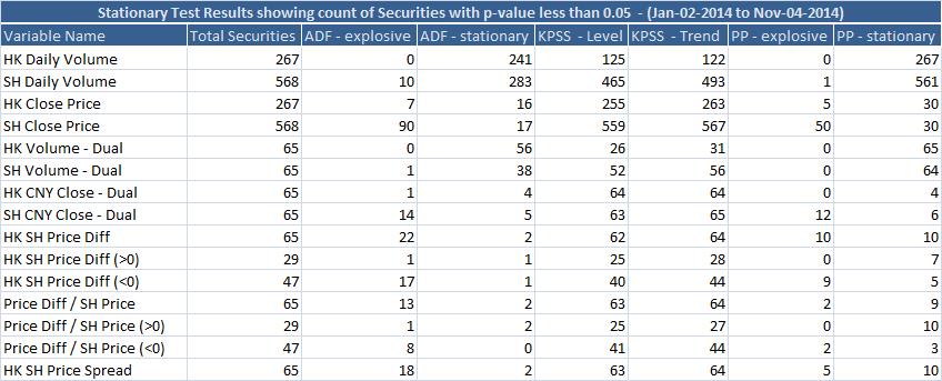
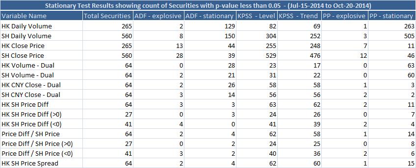
Figure 2: Convergence and Stationary Test Results

4.3.1 Price Premium

The Positive Price Premium on dual listed securities has fallen by more than 100% (Figure 3). The positive price premium is measured as the difference between the Hong Kong Security Price and the Shanghai Security Price as a percentage of the Shanghai price, when the Hong Kong Security Price is greater than the Shanghai Price. While the below is the daily average across securities with a positive premium, we see similar results for the aggregate and also when we take a weighted average based on the volumes traded. The median number of securities with the positive premium varies is 24 and it varies between 20 to 25 over the course of the analysis time period. From the PP stationary test, there are more number of securities here, as a proportion of the total that might have price convergence. This explains the distinct change in the price premium in this group, as compared to the negative premium and the aggregate premium. The negative price premium is defined and treated similarly. The median number of securities with the negative premium is 40 and it varies between 40 to 45 over the course of the analysis time period. We create a price index to show the overall price movement in all the Hong Kong and Shanghai securities that are part of the connect, weighted by market capitalization and the starting value set to one. The Hong Kong price index is higher while the Shanghai price index is not (Figure 3).

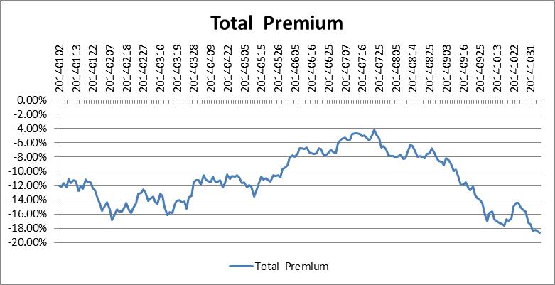
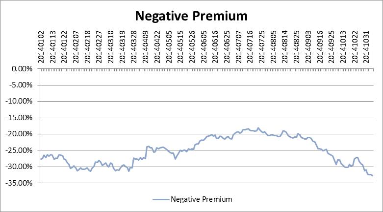
Figure 6: Total and Negative Premium

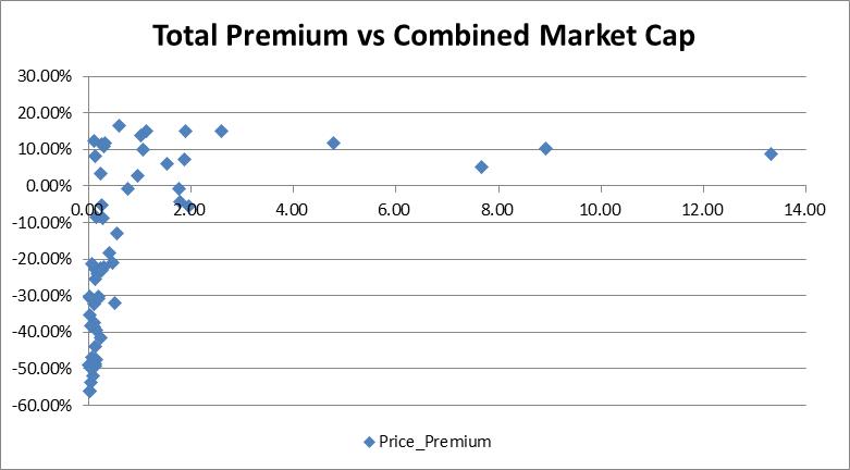
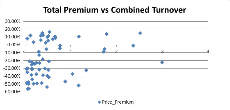
Figure 7: Premium vs Combined Market Cap and Turnover

Additional graphs illustrating the total premium and how the premium is distributed based on Market Cap and Turnover are given in Appendix 8.1 (Figures 6, 7).

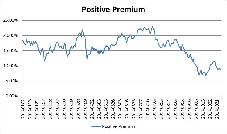
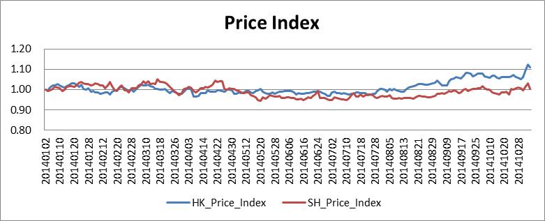
Figure 3: Price Premium and Price Index

4.4 Hong Kong and Shanghai Traded Volume

Volume Traded in Shanghai has gone up by more than 200% (Figure 4). The volume is indexed to one at the start of the time period and the effect of price increases have been removed to capture only the growth in notional traded. Since volume is stationary from the earlier section, we can conclude there is indeed a shift towards higher trading levels.

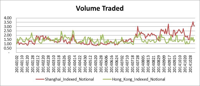
Figure 4: Volume Traded

4.5 Simulated Trading Cost Comparison on Dual Listed Hong Kong and Shanghai Securities

We look at how the trading cost estimates on dual listed securities have changed over the months leading up to the Connect. The simulations used have the same parameters for the Hong Kong security and for the dual listed Shanghai security. We look at the full sample and also slice it into various categories like Side, Market Capitalization, Sector and % ADV demand of the order.

We run time trend regressions of the sort below, where we aggregate the market impact across different buckets by taking the notional weighted average and for comparison purposes, we also consider another version of these regressions just by taking the simple average.

$$\overset{K}{\underset{i=1}{\sum}w_{i}}y_{it}=\beta_{0}+\beta_{1}t+\varepsilon_{t}$$ (60)

Here, $w_{i}$ is the weight of an estimate $y_{it}$ in a particular category being considered at time $t$ with a total of $K$ estimates being aggregated in that bucket.

We perform Welch-T tests across Hong Kong and Shanghai securities for the simple average and notional weighted average trading cost estimates over different buckets. The t statistic for this test, checks the difference in the means of two time series and accounts for the different variances.

$$t\quad=\quad\frac{\;\overline{X}_{1}-\overline{X}_{2}\;}{\sqrt{\;\frac{s_{1}^{2}}{N_{1}}\;+\;\frac{s_{2}^{2}}{N_{2}}\quad}}\,$$ (61)

where $\overline{X}_{i}\text{, }s_{i}^{2}$ and $N_{i}$ are the sample mean, sample variance and sample size, respectively.

We repeat the entire set of tests for the last two months before the event. We perform another set of comparisons excluding liquidity demand 50%+ ADV from the sample since the higher impact orders tend to be larger and would skew the results. This would lead to better conclusions because the number of real orders in these buckets tends to be small, but we can still look at the changes in these higher ADV orders as they will show up separately in the ADV categorization.

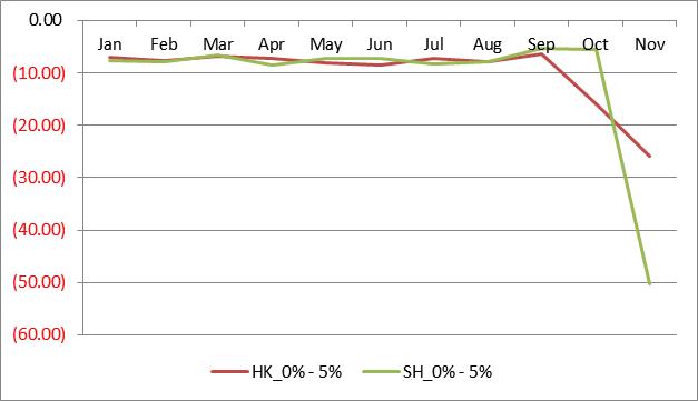
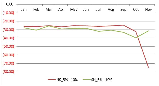
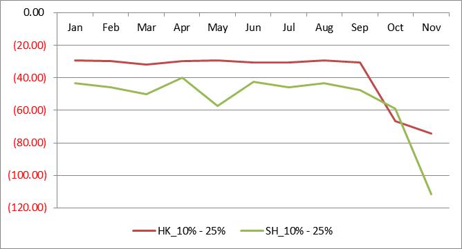
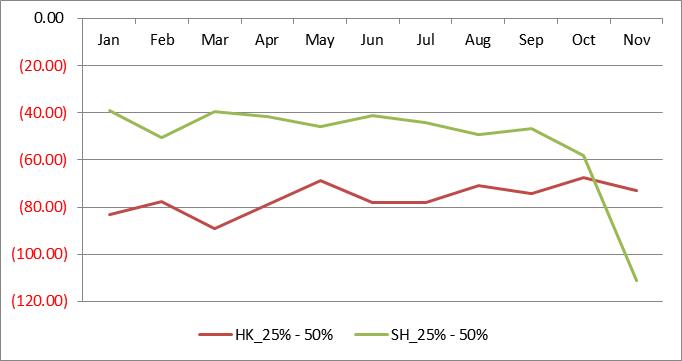
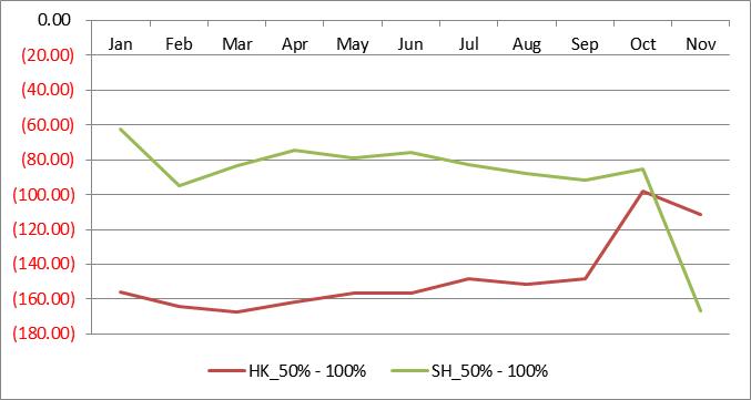
Figure 17: Simulation Trading Costs by % ADV Demand

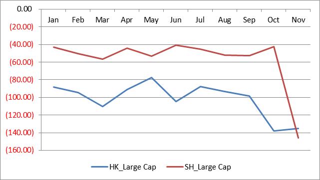
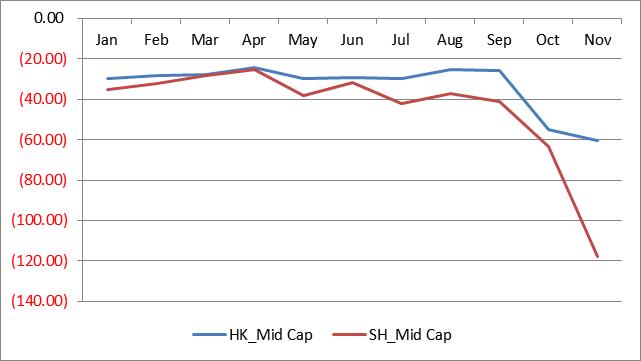
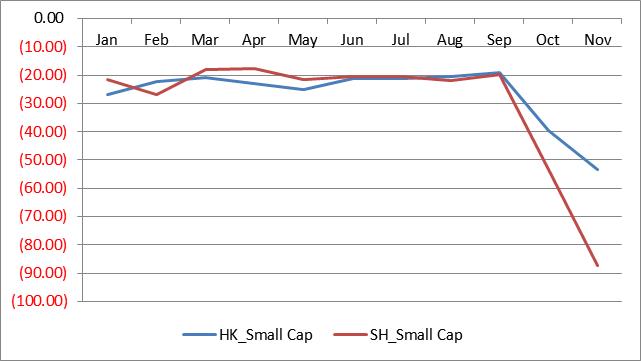
Figure 18: Simulation Trading Costs by Market Capitalization

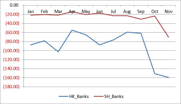
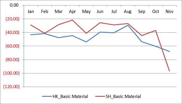
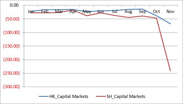
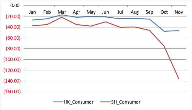
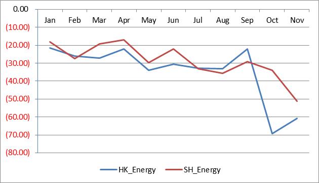
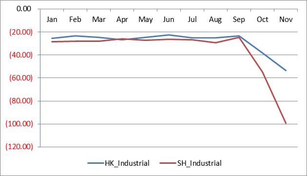
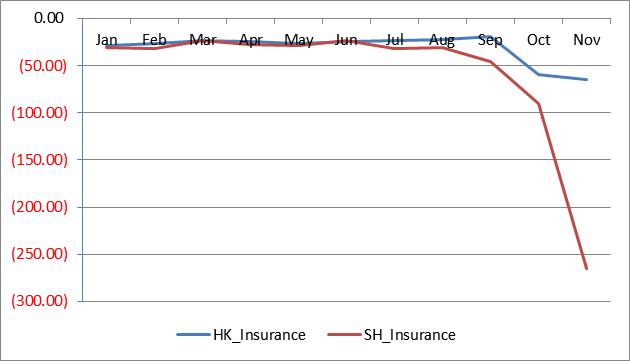
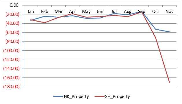
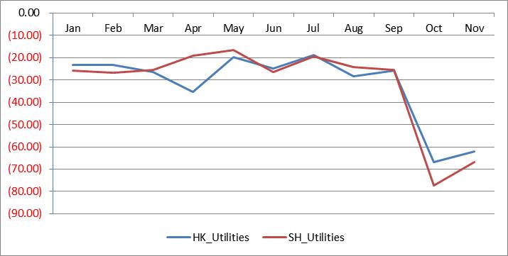
Figure 19: Simulation Trading Costs by Sector

We see that the trading costs in Shanghai on an overall basis are lower than Hong Kong till the days leading up to the connect, but as we get closer to Connect, the costs in Shanghai become higher. We summarize the comparison in figure 5 below. Additional graphs and results are given in Appendix 8.2. Figures 17, 18 and 19 show trading cost trends by liquidity demand, market cap and sectors.

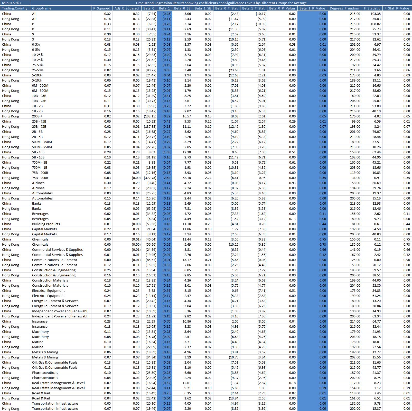
Figure 8: Time Trend Regression - Without 50%+ ADV

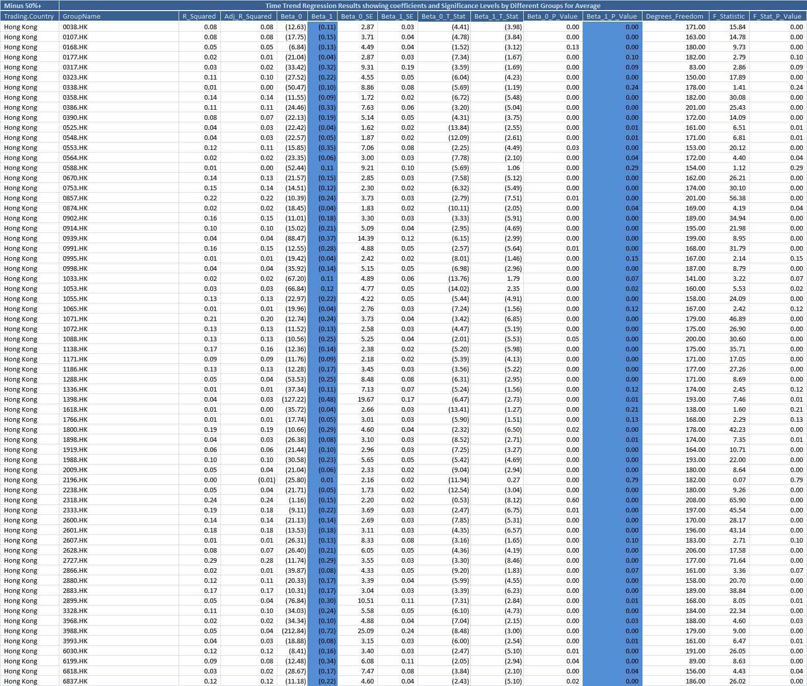
Figure 9: Time Trend Regression - Without 50%+ ADV HK Securities

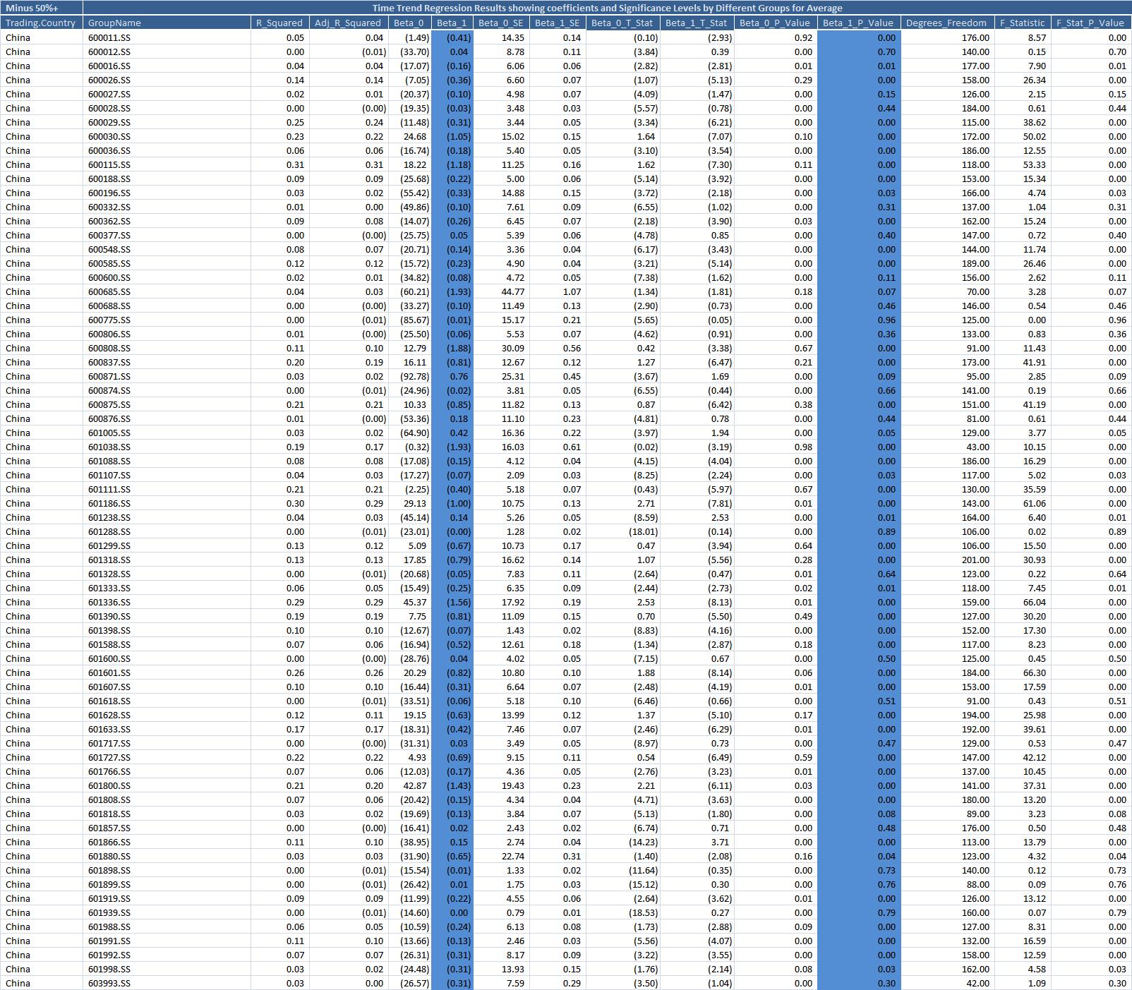
Figure 10: Time Trend Regression - Without 50%+ ADV SH Securities

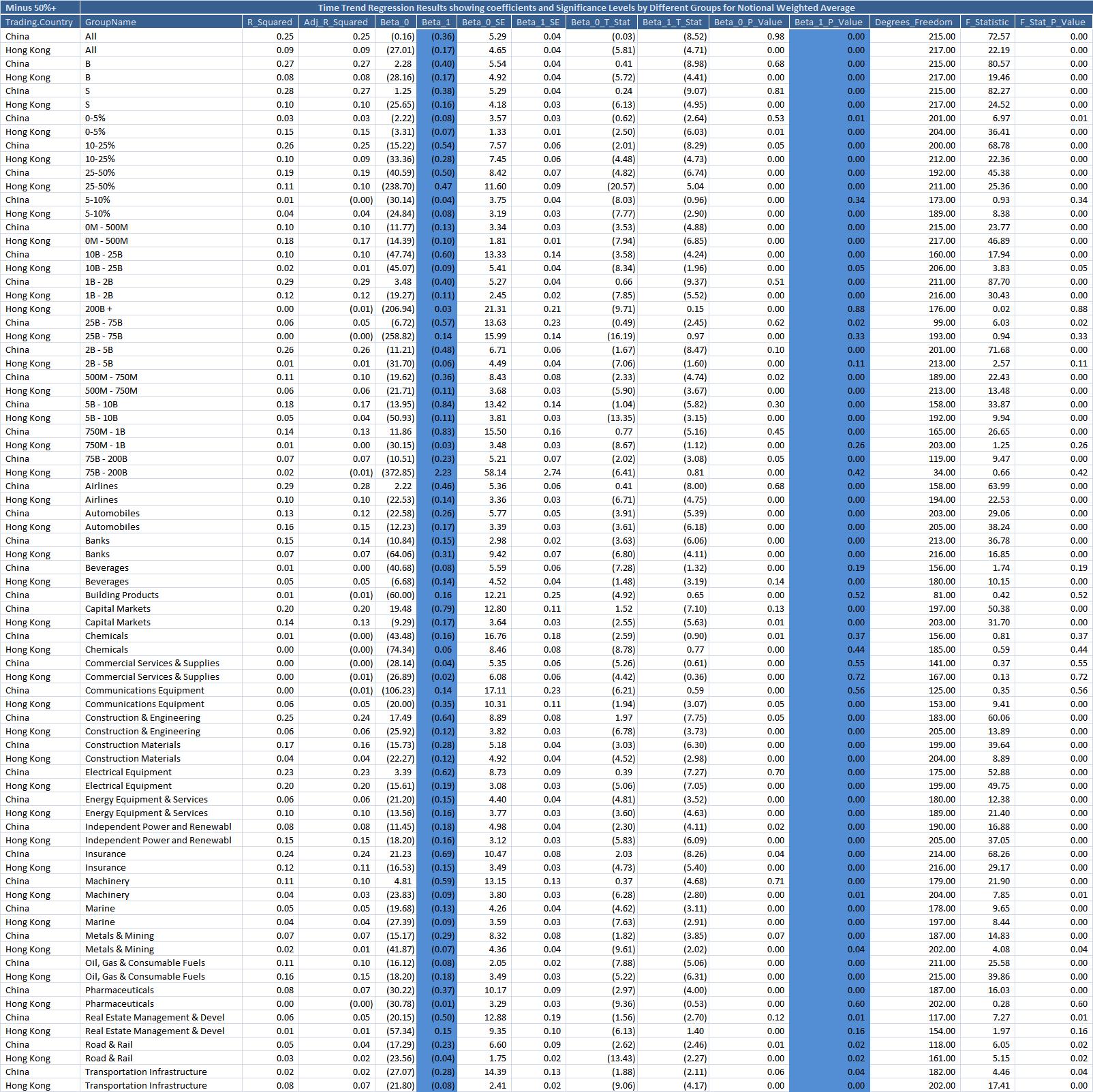
Figure 11: Time Trend Regression - Without 50%+ ADV Notional Weighted

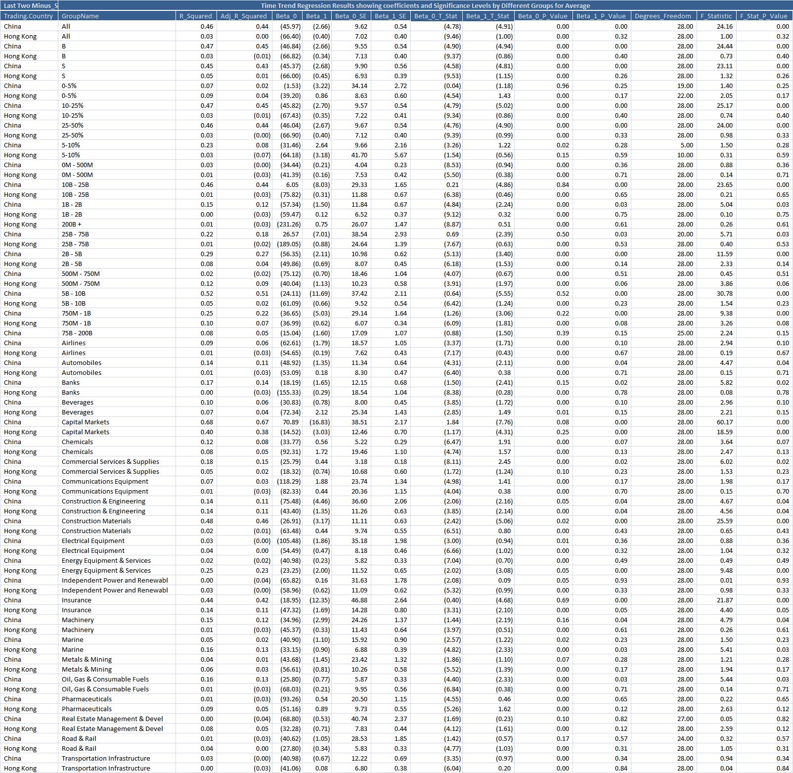
Figure 12: Time Trend Regression - Without 50%+ ADV Last Two Months

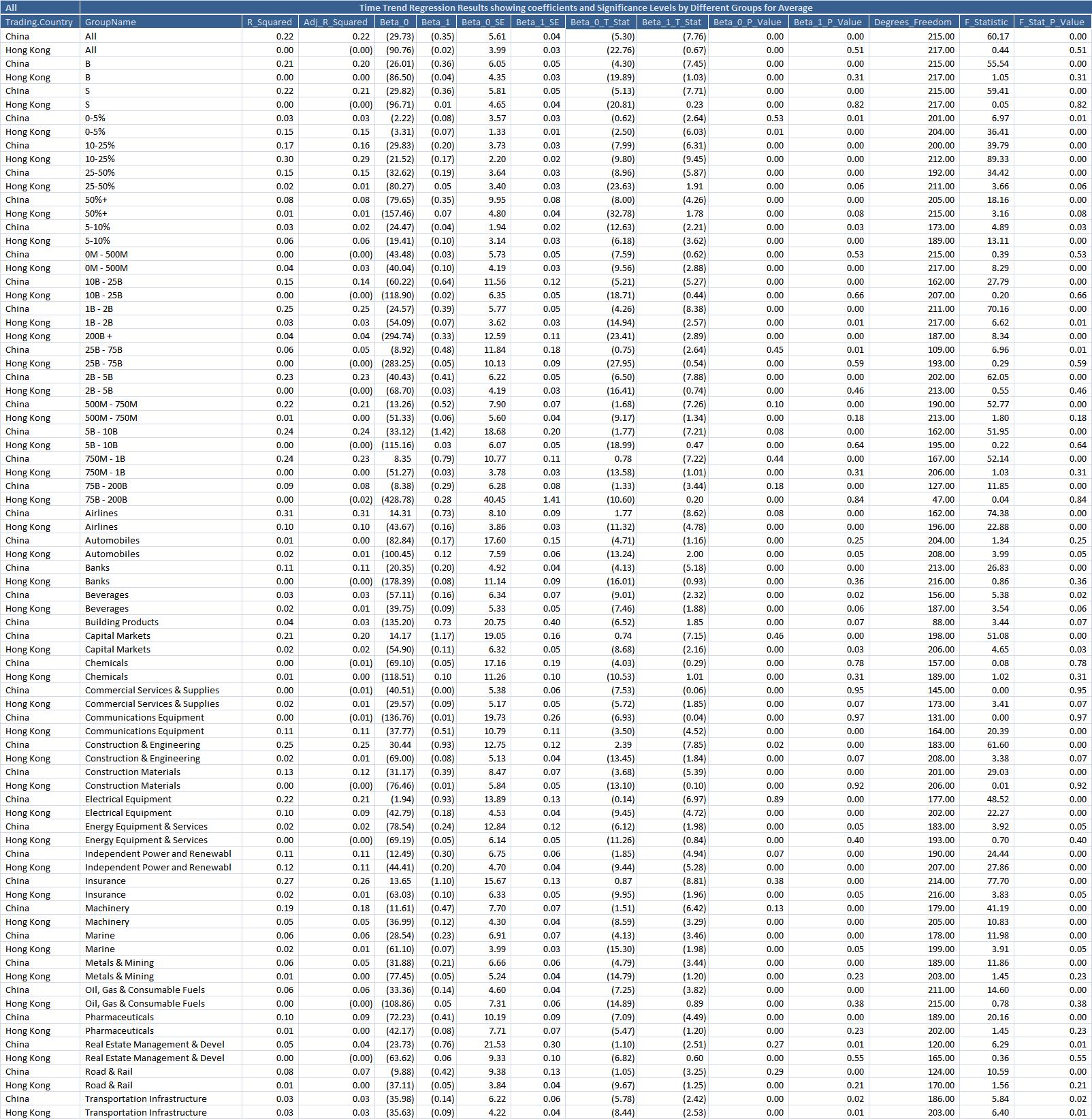
Figure 13: Time Trend Regression - Full Sample

In the time trend regressions, we see more negative coefficients (also, statistically significant) on the China sub-groups as compared to the HK sub-groups. The results are only amplified when we consider the full sample and the notional weighted average. Figures 8, 9, 10, 11 and 12 report the time trend regressions (coefficients and corresponding p-values are highlighted) when 50% ADV orders are excluded by various categories, Hong Kong securities, Shanghai securities, various categories weighted by notional and for the last two months in the sample; Figure 13 is for the full sample including the 50%+ ADV orders.

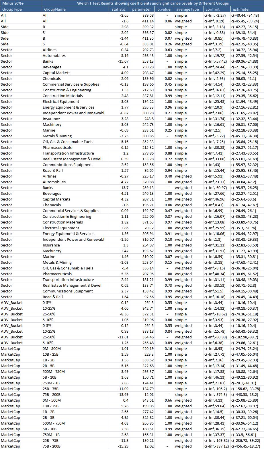
Figure 14: Welch T Test - Without 50%+ ADV

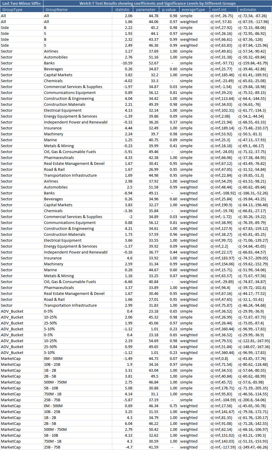
Figure 15: Welch T Test - Without 50%+ ADV Last Two Months

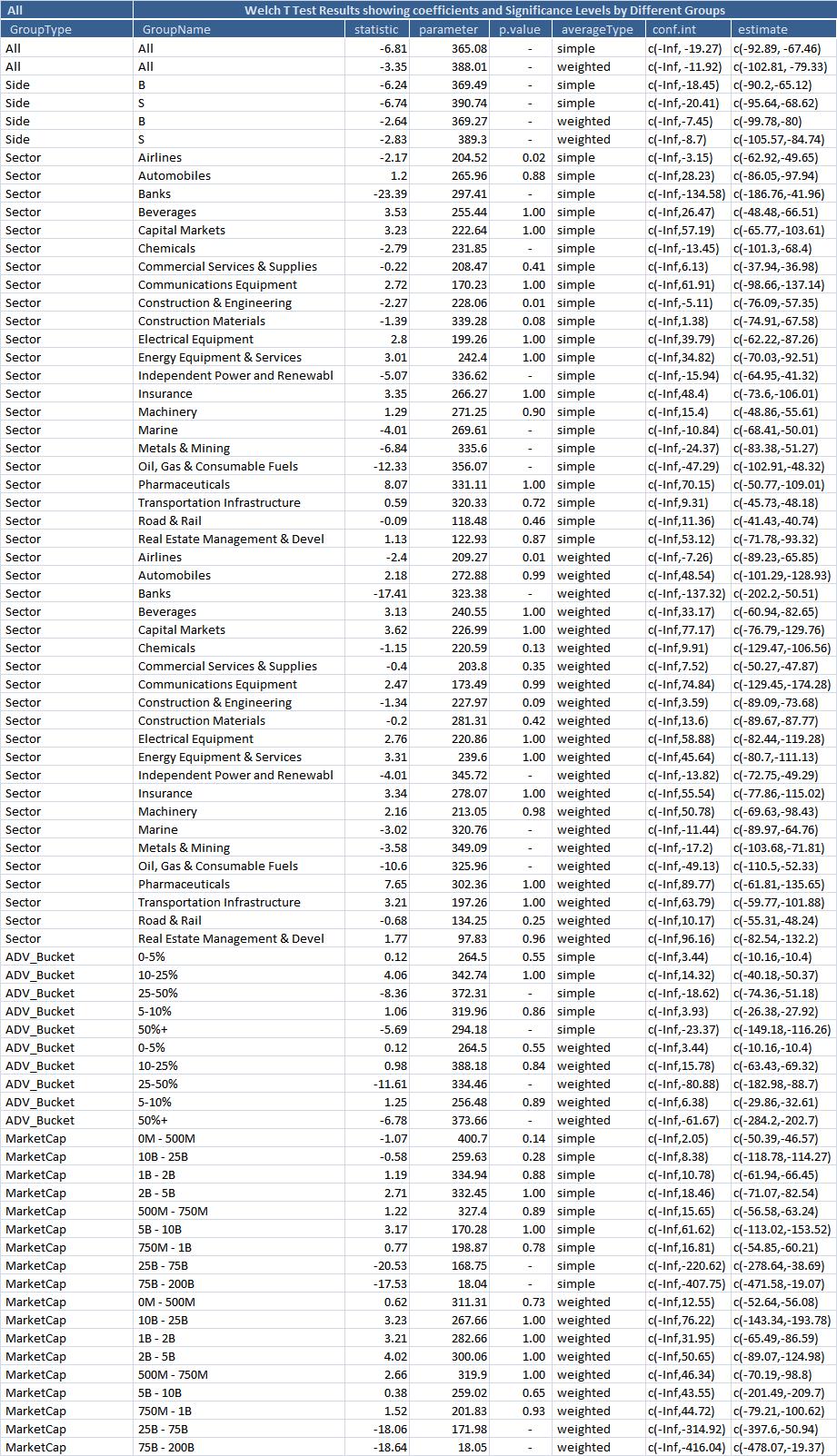
Figure 16: Welch T Test - Full Sample

In the Welch tests we see that the HK means are higher for the overall sample, but in the last two months before the event the China means are higher for the majority of the sub-groups. The last column in Figures 14, 15 and 16 shows the estimates of the mean values of HK and Shanghai, with less than as the alternate hypothesis, when 50% ADV orders are excluded, for the last two months without 50% ADV orders and for the full sample including the 50% ADV orders respectively.

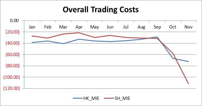
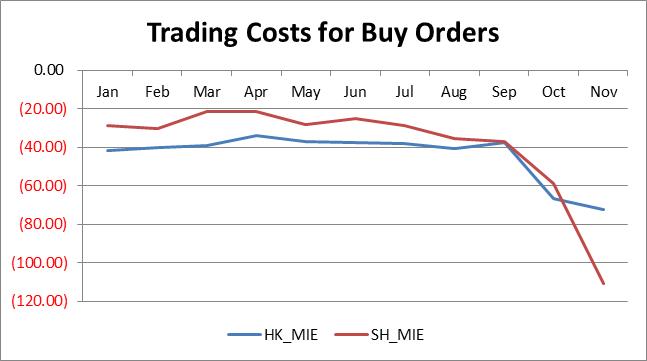
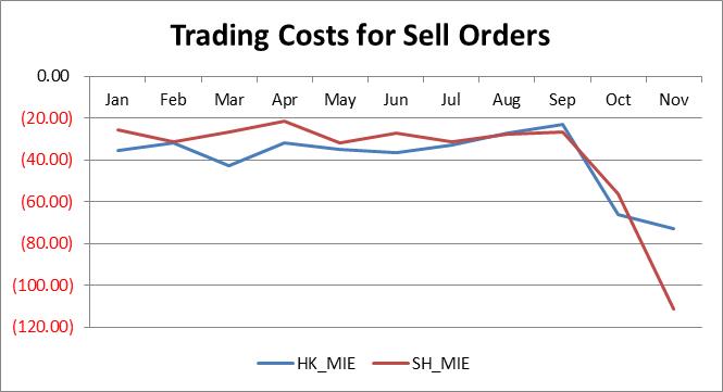
Figure 5: Simulation Trading Costs

4.6 Estimated and Actual Costs across Real Orders on Dual Listed Hong Kong Securities

When doing any study of trading costs, we need to face the realities of high variance and extremely low co-efficient of variations. The key is to extract the signal from the noise being mindful of the fact that if we have a candle in the dark, our mission is accomplished. To aid this effort at amplifying the signals, we filter out orders that show zero market impact since they increase the noise without adding any meaningful explanation. This is also practical from another point since the orders with zero impact are traded very passively and hence their inclusion would only reduce the contribution of orders with meaningful impact towards any patterns we wish to uncover. To differentiate this study from other impact studies that rely significantly on price volatility, we run the test without including price volatility, but use only a dummy variable to include the type of volatility environment. We first run Mincer-Zarnowitz (MZ) type regressions of the type shown below, between the actual impact and the corresponding estimate.

$$y_{t}=\beta_{0}+\beta_{1}\hat{y_{t}}+\varepsilon_{t}$$ (62)

Results of test of hypothesis (both joint and separate) on the estimated coefficients using the F-test of significance for $\beta_{0}=0;\beta_{1}=1$ result in rejection; but with $\beta_{0}=\hat{\beta_{0}}\pm\triangle_{0};\beta_{1}=\hat{\beta_{1}}\pm\triangle_{1}$, that is with small values around the estimated coefficients we get high $p$-values (Hamilton 1994; Gujarati 1995; Verbeek 2008; End-notes 7, 8) implying that the coefficients are significant but have a great deal of sensitivity around their estimated values, an artifact of the high noise environment.

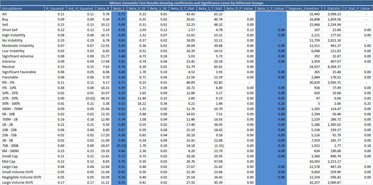
Figure 20: Mincer Zarnowitz Regression Results

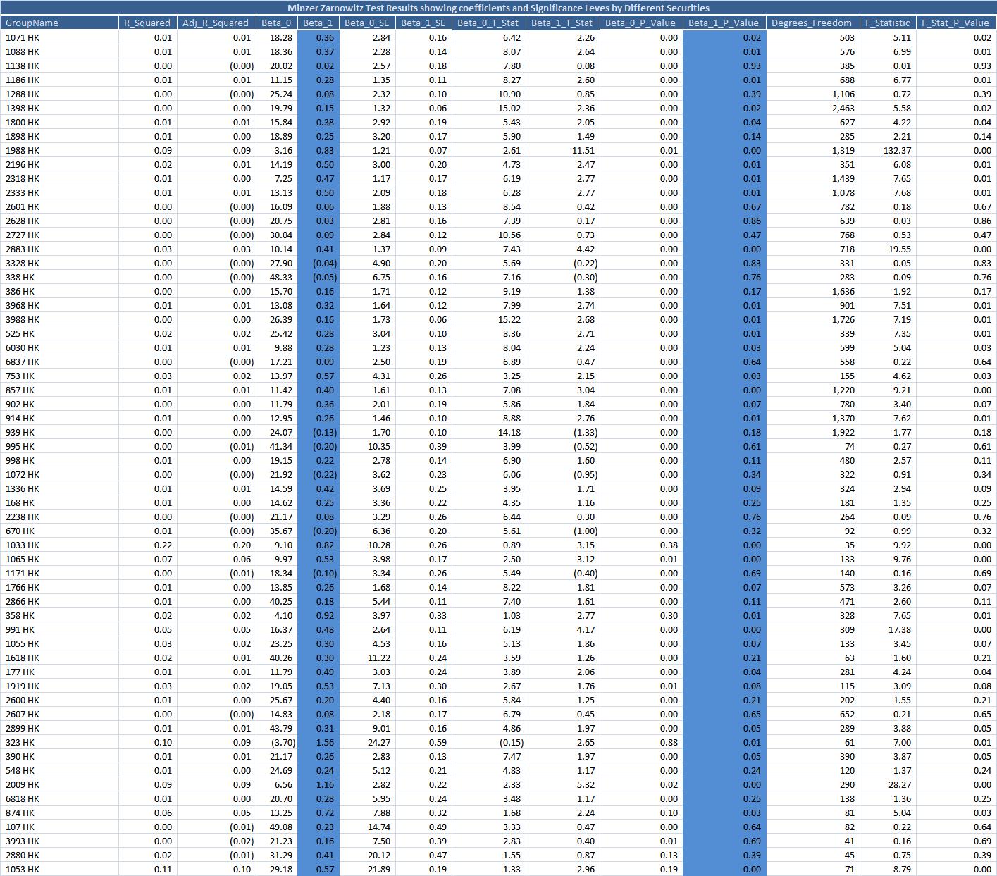
Figure 21: Mincer Zarnowitz Regression Results - HK Securities

We run regressions on the full sample and also with trading costs broken down into various categories similar to the ones we used in the previous section. This allows the comparison of how accurate the estimated costs are versus real costs and helps establish confidence in our estimation methodology. The results (Appendix 8.3) show that the coefficients are non-zero and significant, indicating a good level of forecasting prowess. Figures 20 and 21 highlight the regression coefficients and p-values for different groups and for HK securities.

To understand the upper limits of the predictive ability, we include other variables and run secondary regressions. First we include category variables. We try two flavors of specifications. One with the set of category variables that we know before an order is traded (side, capitalization, sector, liquidity demand). The other set would define the environment when an order is being executed (expected price-momentum, volume and volatility buckets). Other possible variables for the first set are: arrival price, total number of shares, 90-day moving price volatility for each security; for the second set, either as category variables or explicit numerical forecasts, are: expectations regarding notional traded, spread cost, number and size of executions, order duration and security level price trend. This illustrates that specific numerical forecasts of these second set of variables can enhance predictive power, but even a judgment regarding which category might apply will still be helpful towards improving performance.

$$y_{t} =\beta_{0}+\beta_{1}\hat{y_{t}}+\overset{K}{\underset{i=2}{\sum}}\beta_{i}D_{i}+\varepsilon_{t}$$ (63)

Here, $$D_{i}\text{ are dummy variables that define each of our sub groups with a total of }K\text{ subgroups.}$$ (64)

$$y_{t} =\beta_{0}+\beta_{1}\hat{y_{t}}+\overset{K}{\underset{i=2}{\sum}}\beta_{i}D_{i}+ln\left(Shares_{t}\right)+\left(Arrival\;Price_{t}\right)+\left(Moving\;Price\;Volatility_{\left\{t-90,t\right\}}\right)$$ (65)

$$+\left(Other\;Variable\;Expectations_{t}\right)+\varepsilon_{t}$$ (66)

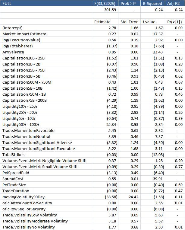
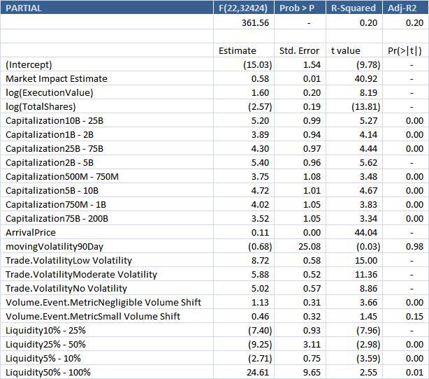
Figure 22: Estimate Regression Results

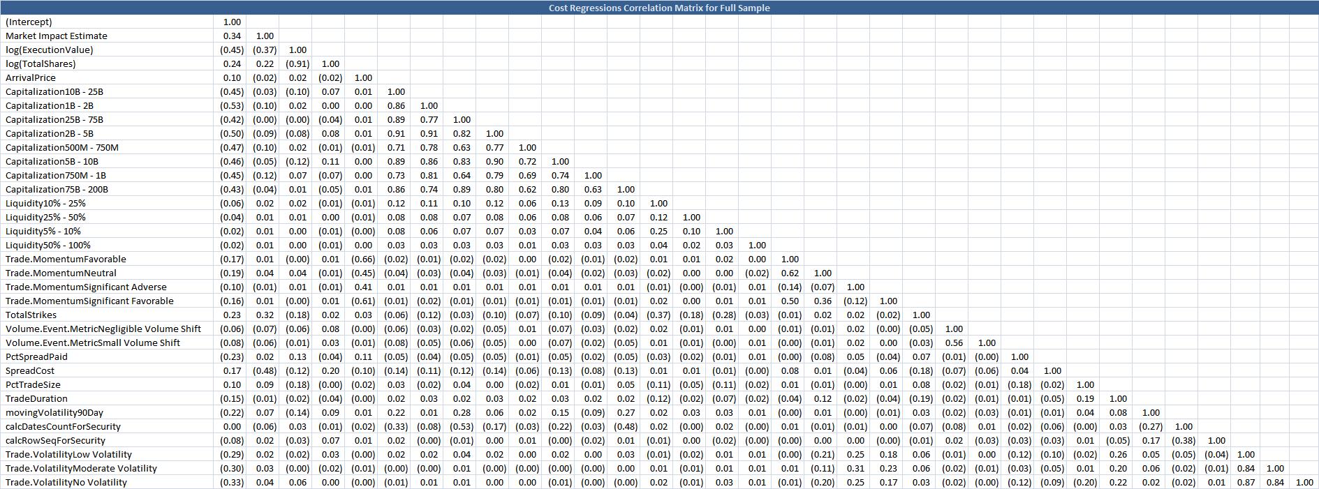
Figure 23: Regression Correlation Matrix

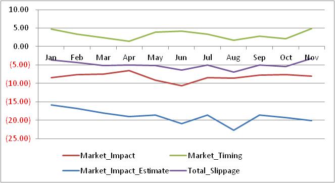
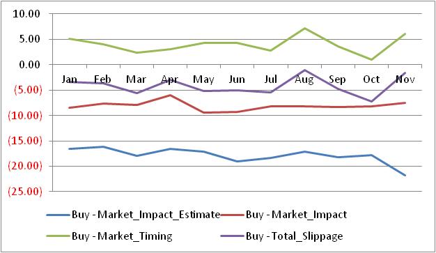
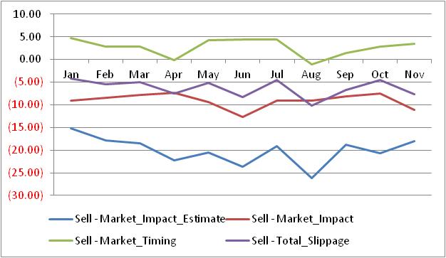
Figure 24: Trading Costs on Real Orders

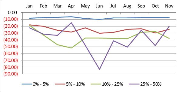
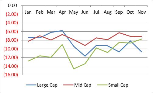
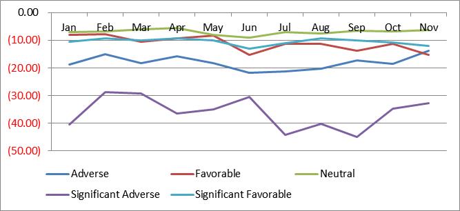
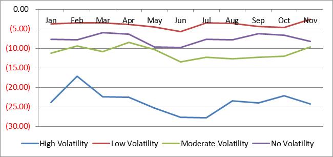
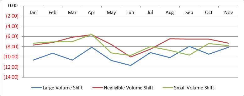
Figure 25: Market Impact Costs on Real Orders

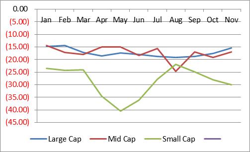
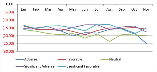
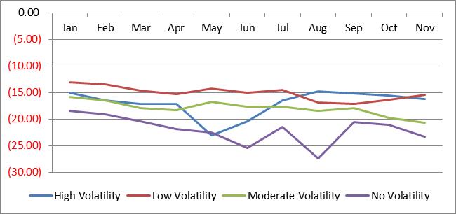
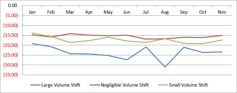
Figure 26: Market Impact Estimate Costs on Real Orders

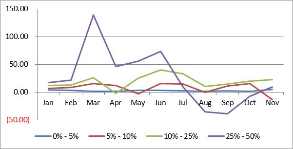
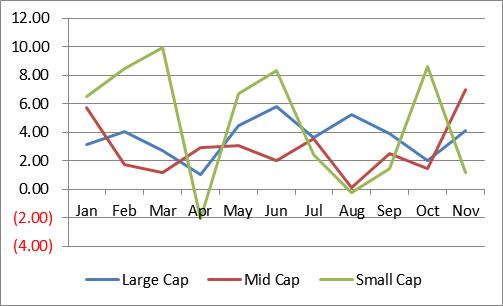
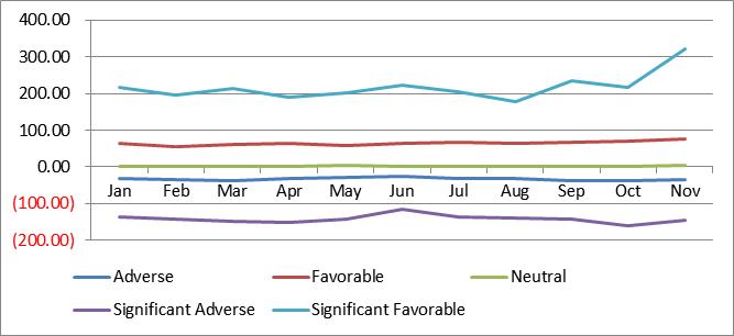
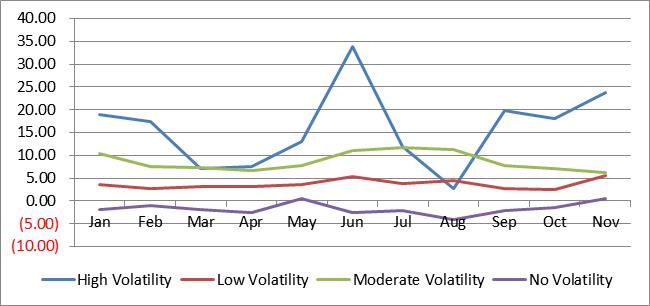
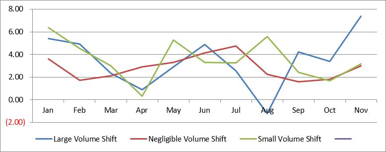
Figure 27: Market Timing Costs on Real Orders

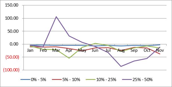
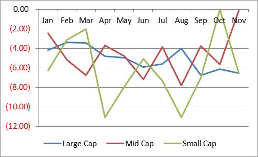
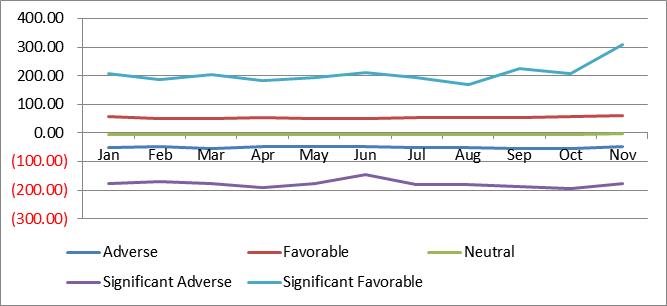
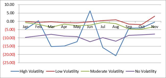
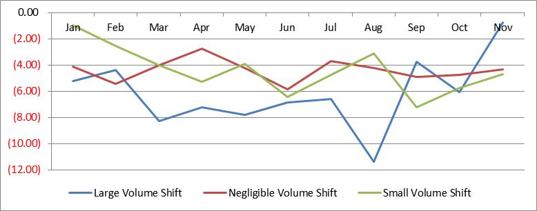
Figure 28: Total Slippage Costs on Real Orders

The evaluation of the forecasts still relies on the basic MZ regression. The other specifications (Figure 22, shows the results for two cuts of variables from among the many alternatives tried) are merely to illustrate the increased explanatory power that comes with our trading cost methodology. The full correlation matrix is in Figure 23. Figures (24, 25, 26, 27 and 28) show time trends of all trading cost variables by side; Market Impact, Market Impact Estimate, Market Timing and Total slippage by various groups.

4.7 Auxiliary Metrics on Real Orders

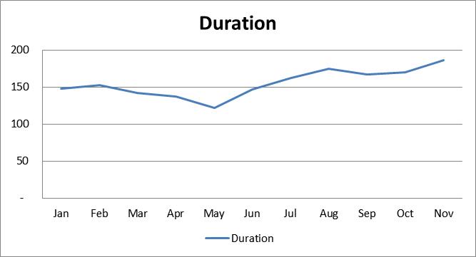
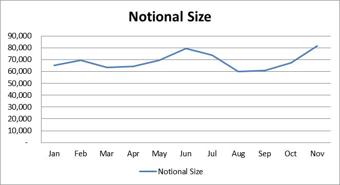
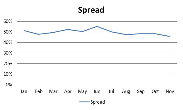
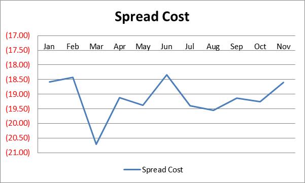
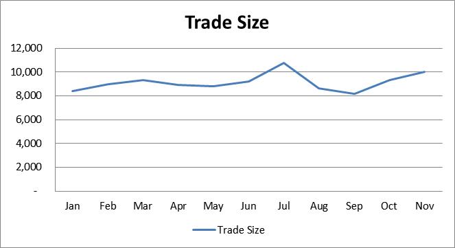
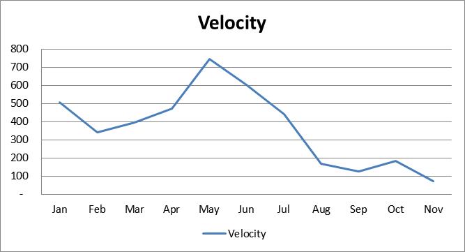
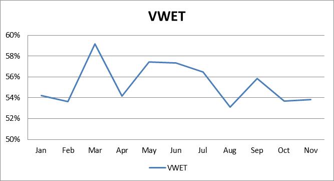
Figure 29: Auxiliary Metrics on Real Orders

The price of liquidity, as measured by the spread, both in terms of the actual value or in terms of percentage of the spread paid has not changed drastically. The size of trades have increased both in shares and notional terms, as has the duration over which orders are traded. The velocity of trading as measured by the number of executions per minute has decreased. This could be an indication of traders grabbing bigger chunks of liquidity but more patiently since they are waiting longer to fill the entire orders. Combining this inference with the Volume Weighted Execution Time (VWET) we find that the trading is still fairly evenly spread out over the duration of the order. VWET indicates the extent to which executions are front loaded or back loaded within the entire order duration. A value close to 50% indicates a fairly even distribution of executions or executions closer to the front or to the back of the order duration. (Appendix 8.4, Figure 29)

4.8 Volume Curves for Select Hong Kong and Shanghai Names

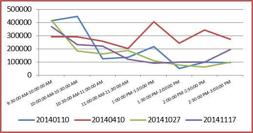
Figure 30: Volume Curves for 0001.HK

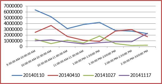
Figure 31: Volume Curves for 0688.HK

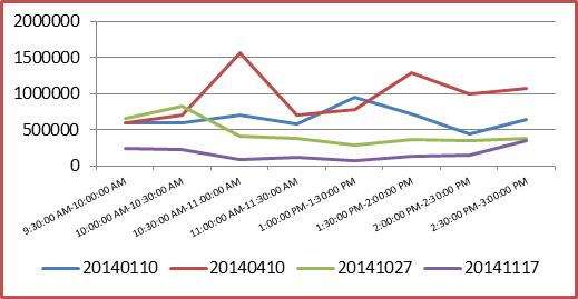
Figure 32: Volume Curves for 0813.HK

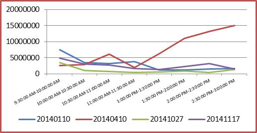
Figure 33: Volume Curves for 0992.HK

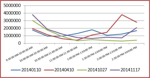
Figure 34: Volume Curves for 1928.HK

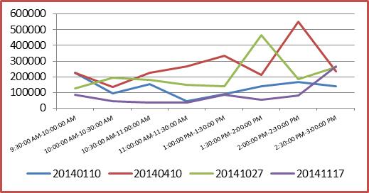
Figure 35: Volume Curves for 0669.HK

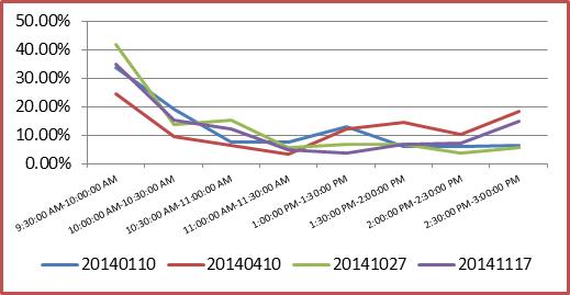
Figure 36: Volume Curves for 0700.HK

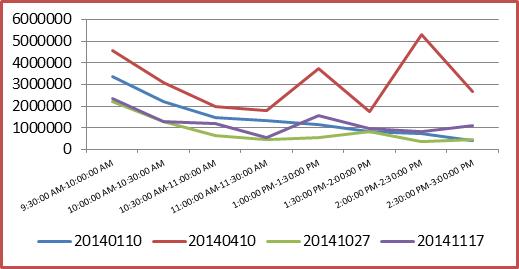
Figure 37: Volume Curves for 0941.HK

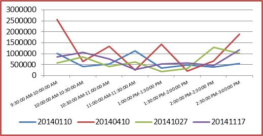
Figure 38: Volume Curves for 1114.HK

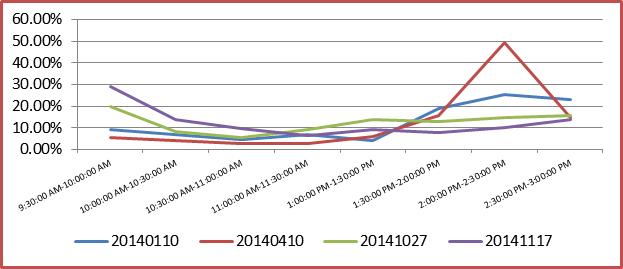
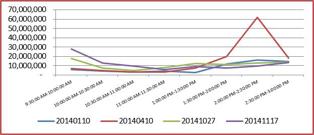
Figure 40: Volume Curves for 600036.SS

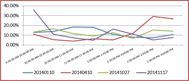
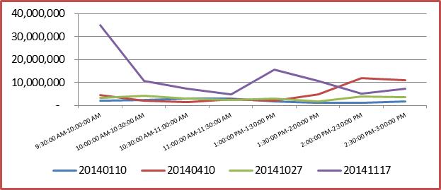
Figure 41: Volume Curves for 600104.SS

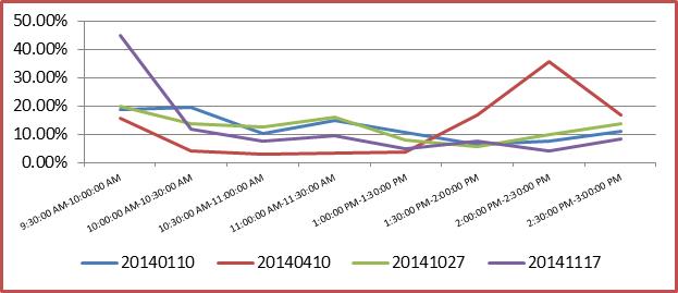
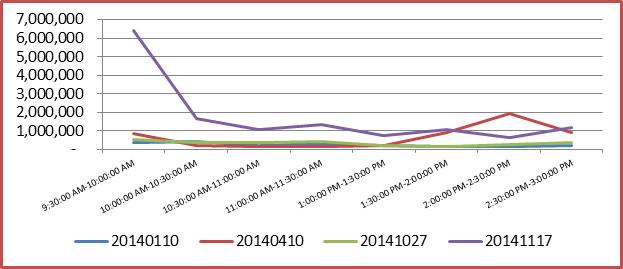
Figure 42: Volume Curves for 600519.SS

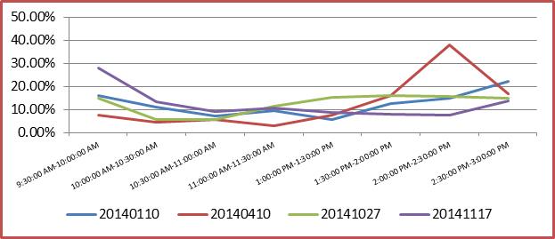
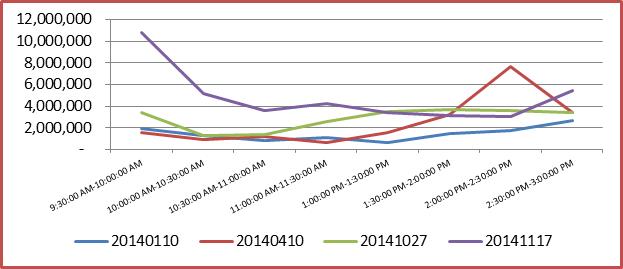
Figure 43: Volume Curves for 600900.SS

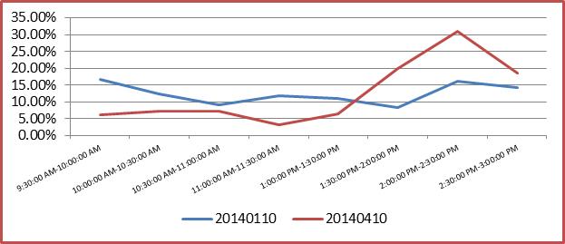
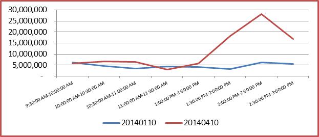
Figure 44: Volume Curves for 601299.SS

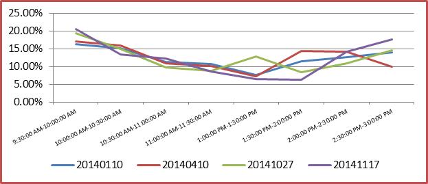
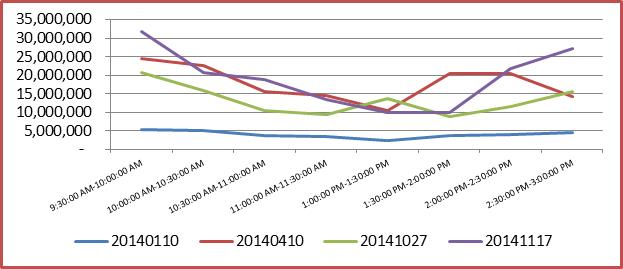
Figure 45: Volume Curves for 600048.SS

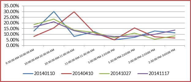
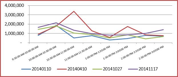
Figure 46: Volume Curves for 600372.SS

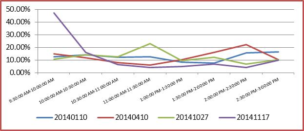
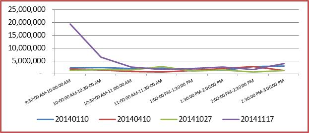
Figure 47: Volume Curves for 600690.SS

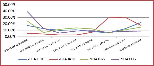
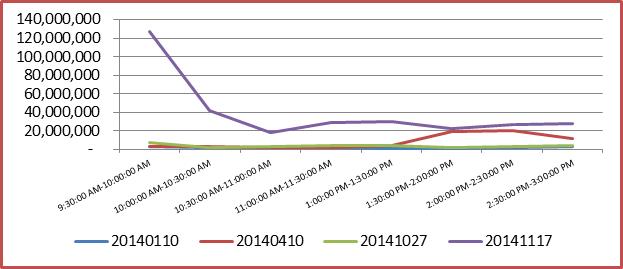
Figure 48: Volume Curves for 601006.SS

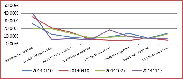
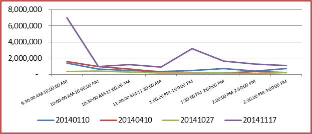
Figure 49: Volume Curves for 601888.SS

Volume Curves across key dates leading up to the Connect are shown for a select number of single names. It is fairly easy to infer that the volumes traded increase significantly around announcement dates and on the launch date of the Connect. We show the volume both as percentage of day’s total volume and in number of shares. (Appendix 8.5, Figures 30-49)

5 Conclusions and Possibilities for Future Research

Adhering to a modified version of the old adage, “A picture is equal to a thousand words or a million numbers (or pixels)”, we have presented, where possible, some of the main empirical results as easy to read graphs supplementing the analysis with statistical tests, explanations and highlighting major observations. One conclusion that emerges is that the trading costs in Shanghai which might have been cheaper compared to Hong Kong might be becoming more expensive in the run up to the Connect and perhaps even beyond. Contrary to what one would except, given the increasing trading volume and converging price premium, the divergence of trading costs stands out as an interesting effect of the greater demand for liquidity on the northbound route. What remains to be seen and analyzed in later studies is whether this increase in trading costs is a temporary equilibrium due to the frenzy to gain exposure to Chinese securities or whether this phenomenon will persist once the two markets start becoming more and more tightly coupled. Also of interest would be to see whether other regulatory interventions in the financial markets will lead to such drastic changes to the costs of trading.

In terms of methodology, different statistical procedures can be employed in lieu of Welch type tests. (Welch 1938) considers in detail, tests of hypothesis that the means of two normal populations are equal. Yuen-Welch test (Yuen 1974); Brunner-Munzel test (Brunner and Munzel 2000); and Wilcoxon–Mann–Whitney test (Wilcoxon 1945; Mann and Whitney 1947) are some alternatives. (Fagerland and Sandvik 2009) compare the performance of different tests for skewed distributions with unequal variances. (Fagerland 2012) confirms that the Welch’s t-test remains robust for skewed distributions and large sample sizes.

(Patton and Timmermann 2007a) study different tests of forecast optimality and establish new testable properties that hold when the forecaster’s loss function is unknown. (Patton and Timmermann 2007b) consider asymmetric and nonlinear loss functions. (Elliott and Timmermann 2008) discuss the central role of the loss function in helping determine the forecaster’s objectives. They concede that the menu of forecasting methodologies (none of which may coincide with the “true” model) has expanded vastly over the last few decades. No single approach is currently dominant and the choice of forecasting method is often dictated by the situation at hand such as the forecast user’s particular needs, data availability, and expertise in experimenting with different classes of models and estimation methods. (Patton and Timmermann 2010) find that dispersion among forecasters views is highest at long horizons. Our trading cost methodology is based on the philosophy of short horizon forecasts, and hence the simplicity of the MZ regression might be adequate for our high variance environment. But we leave the door open to considering variations to all the statistical methodologies we have employed, which might show interesting results.

Once the actual connect program starts, we expect to have a significant number of orders traded on securities listed in Shanghai through the Connect. This will allow subsequent studies to do an actual comparison on real orders of which market offers the better way to gain exposure to similar securities from both a trading and also from a portfolio construction perspective. Finally, as an afterthought we let the reader ponder about what financial liberalizations means to the mode of governance in a country. It might be an interesting study to look at other cases where there have been significant changes to the extent of cross border flows of capital and what effect it has had on the economy and the overall well-being of the representative population (See Boyer and Drache 1996; Kashyap 2015a; Quinn 2000; Simmons, Dobbin and Garrett 2008). A related question is the effect, the mode of governance and other aspects of life in one country have on another country, once they start linking up their financial markets.

5.1 Postscript

Since the launch of the connect, the trading volume has not been as high as anticipated, though the program is claimed to be safe, stable and a trend setter for similar partnerships being tabled globally, despite some unresolved issues regarding beneficial and foreign ownership rights, tax treatment on share gains and the custody of assets (End-notes 5, 6).

6 Acknowledgements and End-notes

1. The author would like to express his gratitude to Brad Hunt, Henry Yegerman, Samuel Zou and Alex Gillula at Markit; Patrick Lawlor, Joanna Wong and Eugene Kanvesky at CLSA, for many inputs during the creation of this work. Dr. Yong Wang, Dr. Isabel Yan, Dr. Vikas Kakkar, Dr. Fred Kwan, Dr. Srikant Marakani, Dr. Costel Daniel Andonie, Dr. Jeff Hong, Dr. Guangwu Liu, Dr. Humphrey Tung and Dr. Xu Han at the City University of Hong Kong provided advice and more importantly encouragement to explore and where possible apply cross disciplinary techniques. The views and opinions expressed in this article, along with any mistakes, are mine alone and do not necessarily reflect the official policy or position of either of my affiliations or any other agency.

2. In 2013, China’s real GDP grew by 7.7 %, the same as in 2012. Since 2010, the economic growth rate has declined for four consecutive years (Fig. 2.1). Quite similar to the macroeconomic trends and policy control mode adopted in 2012, from mid-2013, the central government launched a series of fine-tuning measures to stabilize the economic growth rate after experiencing sustained downward growth during the first half of 2013. These measures inhibited the declining economic trend in the third and fourth quarters and ensured that the annual economic growth rate for the entire year matched that of the previous year. However, the real annual growth rate of industrial value added was only 9.7 %, a decrease of 0.3 percentage points from 2012, and the lowest since 2009. A constant drop in the growth rate of industrial value added reflects a slowdown in the real economy (Center for Macroeconomic Research of Xiamen University 2015; A Review of China’s Economy in 2013. Center for Macroeconomic Research, Xiamen University. China’s Macroeconomic Outlook. Springer).

3. What is stock connect? A unique collaboration between the Hong Kong, Shanghai and Shenzhen Stock Exchanges, Stock Connect allows international and Mainland Chinese investors to trade securities in each other’s markets through the trading and clearing facilities of their home exchange. What is stock connect?

4. Sergey Nazarovich Bubka (born 4 December 1963) is a Ukrainian former pole vaulter. He represented the Soviet Union until its dissolution in 1991. Sergey has also beaten his own record 14 times. He was the first pole vaulter to clear 6.0 metres and 6.10 metres. Bubka was twice named Athlete of the Year by Track & Field News and in 2012 was one of 24 athletes inducted as inaugural members of the International Association of Athletics Federations Hall of Fame. Sergey Bubka, Wikipedia Link

5. The gong simultaneously sounded in Shanghai Stock Exchange (SSE) and Hong Kong Exchanges and Clearing Limited (HKEx) on Nov. 17 last year declared the official launch of Shanghai-Hong Kong Stock Connect that links the capital markets of the Chinese mainland and the world. Since then, direct investment access to the stock markets in Shanghai and Hong Kong is available. The stock market of the Chinese mainland is directly open to global capital for the first time, while investors from the Chinese mainland also start their way of global asset allocation. SSE and HKEx report us the performance of the Shanghai-Hong Kong Stock Connect at its anniversary. Though the overall transaction is not really hot, but the program is “stable and safe” in operation and demonstrates the whole world that such open model of capital market with joint regulation from both sides, two-way access, closed operation and controllable risk, pioneered by the Shanghai-Hong Kong Stock Connect, is completely feasible. Shanghai-Hong Kong Stock Connect brings butterfly effect

6. The establishment of Shanghai-Hong Kong Stock Connect is a ground-breaking initiative to both Mainland and Hong Kong as it has, for the first time, enabled mutual market access by investors in the two markets through an orderly, controllable and expandable channel. More importantly, this initiative has paved the way for the opening up of the Mainland’s capital account and helped promote the internationalization of Renminbi and development of the Hong Kong’s capital market. Shanghai-Hong Kong Stock Connect … for Investors

7. F-Test statistic: The test for the hypotheses,

   $$\boldsymbol{H_{0}} :\mu=k$$

   $$\boldsymbol{H_{A}} :\mu\neq k$$

   can be based on the F ratio,

   $$F =\frac{\text{Explained Variance}}{\text{Unexlpained Variance}}=\frac{\text{Between-Group Variability}}{\text{Within Group Variability}}$$

   $$=\frac{n\left(\bar{Y}-k\right)^{2}}{S^{2}}\sim\left\{\begin{array}[]{c}F\left(1,n-1\text{ Degrees of Freedom}\right)\text{ If }\boldsymbol{H_{0}}\text{ is true}\\ \text{ Bigger}\qquad\qquad\qquad\qquad\text{ If }\boldsymbol{H_{A}}\text{ is true}\end{array}\right.$$

   The p-value is the probability of such an ’extreme’ value of the test statistic when $\boldsymbol{H_{0}}$ is true. This is the upper tail area of the $F$$\left(1,n-1\right)$ distribution. This p-value is interpreted in exactly the same way as other p-values:

   1. The smaller the p-value, the stronger the evidence that the null hypothesis does not hold – i.e. that is $\mu$ not equal to $k$.

   2. A large p-value (say 0.1 or higher) means that the data are consistent with $\mu$ being equal to $k$.

   P-Value for F-Test; F-Test, Wikipedia Link

8. In general, if p-value is less than a critical value then reject the null hypothesis. Less is usually a p-value of 0.05 or lower. This would mean testing at the 5% significance level.

   1. For Stationary Tests, (ADF, PP, KPSS), the following are the null and alternative hypotheses:

   2. In ADF and PP, we specify the alternate hypothesis, stationary or explosive. (Null is Unit Root).

   3. In KPSS, we specify the null hypothesis, Level or Trend Stationary. (Alternative is Unit Root).

   Augmented Dickey-Fuller Test, Wikipedia Link; Phillips–Perron Test, Wikipedia Link; KPSS-Test, Wikipedia Link

7 References

1. Almgren, R., & Chriss, N. (2001). Optimal execution of portfolio transactions. Journal of Risk, 3, 5-40.

2. Almgren, R. F. (2003). Optimal execution with nonlinear impact functions and trading-enhanced risk. Applied mathematical finance, 10(1), 1-18.

3. Almgren, R., Thum, C., Hauptmann, E., & Li, H. (2005). Direct estimation of equity market impact. Risk, 18, 5752.

4. Beck, T., & Levine, R. (2004). Stock markets, banks, and growth: Panel evidence. Journal of Banking & Finance, 28(3), 423-442.

5. Bedi, J., Richards, A. J., & Tennant, P. (2003). The characteristics and trading behavior of dual-listed companies. Reserve Bank of Australia Research Discussion Paper, (2003-06).

6. Bekaert, G., Harvey, C. R., & Lundblad, C. (2005). Does financial liberalization spur growth?. Journal of Financial economics, 77(1), 3-55.

7. Bekaert, G., Harvey, C. R., & Lundblad, C. (2007). Liquidity and expected returns: Lessons from emerging markets. Review of Financial Studies, 20(6), 1783-1831.

8. Bernard, A. B., & Durlauf, S. N. (1995). Convergence in international output. Journal of applied econometrics, 10(2), 97-108.

9. Bernard, A. B., & Durlauf, S. N. (1996). Interpreting tests of the convergence hypothesis. Journal of econometrics, 71(1), 161-173.

10. Bhargava, A. (1986). On the theory of testing for unit roots in observed time series. The Review of Economic Studies, 53(3), 369-384.

11. Brunner, E., & Munzel, U. (2000). The nonparametric Behrens-Fisher problem: Asymptotic theory and a small-sample approximation. Biometrical Journal, 42(1), 17-25.

12. Boyer, R. & Drache, D. (Eds.). (1996). States against markets: the limits of globalization. York University. University of Toronto. Innis College (Toronto). London: Routledge.

13. Center for Macroeconomic Research of Xiamen University. (2015). A Review of China’s Economy in 2013. In: China’s Macroeconomic Outlook. Current Chinese Economic Report Series. pp 7-18. Springer, Berlin, Heidelberg.

14. Collins, B. M., & Fabozzi, F. J. (1991). A methodology for measuring transaction costs. Financial Analysts Journal, 47(2), 27-36.

15. Deeg, R., & O’Sullivan, M. A. (2009). The political economy of global finance capital. World Politics, 61(04), 731-763.

16. De Jong, A., Rosenthal, L., & Van Dijk, M. A. (2003). The limits of arbitrage: evidence from dual-listed companies. Erasmus University working paper.

17. De Jong, A., Rosenthal, L., & Van Dijk, M. A. (2009). The Risk and Return of Arbitrage in Dual-Listed Companies*. Review of Finance, 13(3), 495-520.

18. Dickey, D. A., & Fuller, W. A. (1979). Distribution of the estimators for autoregressive time series with a unit root. Journal of the American statistical association, 74(366a), 427-431.

19. Elliott, G., & Timmermann, A. (2008). Economic Forecasting. Journal of Economic Literature, 46(1), 3-56.

20. Epstein, G. A. (Ed.). (2005). Financialization and the world economy. Edward Elgar Publishing. Cheltenham, UK.

21. Fagerland, M. W., & Sandvik, L. (2009). Performance of five two-sample location tests for skewed distributions with unequal variances. Contemporary clinical trials, 30(5), 490-496.

22. Fagerland, M. W. (2012). t-tests, non-parametric tests, and large studies—a paradox of statistical practice?. BMC medical research methodology, 12(1), 1.

23. Fong, T., Wong, A., & Yong, I. (2008). Share price disparity in Chinese stock markets. Macroeconomic Linkages between Hong Kong and Mainland China.

24. Greasley, D., & Oxley, L. (1997). Time-series based tests of the convergence hypothesis: some positive results. Economics Letters, 56(2), 143-147.

25. Greene, W. H. (2003). Econometric analysis. Pearson Education India.

26. Gromb, D., & Vayanos, D. (2010). Limits of Arbitrage. Annual Review of Financial Economics, 2(1), 251-275.

27. Gujarati, D. N. (1995). Basic econometrics, 3rd. International Edition.

28. Hamilton, J. D. (1994). Time series analysis (Vol. 2). Princeton university press.

29. Henry, P. B. (2000). Do stock market liberalizations cause investment booms?. Journal of Financial economics, 58(1), 301-334.

30. Kashyap, R. (2014a). Dynamic Multi-Factor Bid–Offer Adjustment Model. The Journal of Trading, 9(3), 42-55.

31. Kashyap, R. (2014b). The Circle of Investment. International Journal of Economics and Finance, 6(5), 244-263.

32. Kashyap, R. (2015a). Financial Services, Economic Growth and Well-Being: A Four Pronged Study. Indian Journal of Finance, 9(1), 9-22.

33. Kashyap, R. (2015b). A Tale of Two Consequences. The Journal of Trading, 10(4), 51-95.

34. Kashyap, R. (2015c). David vs Goliath (You against the Markets), A Dynamic Programming Approach to Separate the Impact and Timing of Trading Costs. Working Paper.

35. Kissell, R. (2006). The expanded implementation shortfall: Understanding transaction cost components. The Journal of Trading, 1(3), 6-16.

36. Kwiatkowski, D., Phillips, P. C., Schmidt, P., & Shin, Y. (1992). Testing the null hypothesis of stationarity against the alternative of a unit root: How sure are we that economic time series have a unit root?. Journal of econometrics, 54(1-3), 159-178.

37. Levine, R. (2001). International financial liberalization and economic growth. Review of International economics, 9(4), 688-702.

38. Levine, R., & Zervos, S. (1996). Stock market development and long-run growth. The World Bank Economic Review, 10(2), 323-339.

39. Levine, R., & Zervos, S. (1998a) Stock Markets, Banks, and Economic Growth. American economic review. 88(3), 537-558.

40. Levine, R., & Zervos, S. (1998b). Capital control liberalization and stock market development. World Development, 26(7), 1169-1183.

41. Mann, H. B., & Whitney, D. R. (1947). On a test of whether one of two random variables is stochastically larger than the other. The annals of mathematical statistics, 50-60.

42. Mincer, J. A., & Zarnowitz, V. (1969). The evaluation of economic forecasts. In Economic Forecasts and Expectations: Analysis of Forecasting Behavior and Performance (pp. 3-46). NBER.

43. Patton, A. J., & Timmermann, A. (2007a). Testing Forecast Optimality Under Unknown Loss. Journal of the American Statistical Association, 102(480), 1172-1184.

44. Patton, A. J., & Timmermann, A. (2007b). Properties of optimal forecasts under asymmetric loss and nonlinearity. Journal of Econometrics, 140(2), 884-918.

45. Patton, A. J., & Timmermann, A. (2010). Why do forecasters disagree? Lessons from the term structure of cross-sectional dispersion. Journal of Monetary Economics, 57(7), 803-820.

46. Peng, W., Miao, H., & Chow, N. (2008). Price convergence between dual-listed A and H shares. Macroeconomic Linkages between Hong Kong and Mainland China, 295-315.

47. Perold, A. F. (1988). The implementation shortfall: Paper versus reality. The Journal of Portfolio Management, 14(3), 4-9.

48. Phillips, P. C., & Perron, P. (1988). Testing for a unit root in time series regression. Biometrika, 75(2), 335-346.

49. Quinn, D. P. (2000). Democracy and international financial liberalization. McDonough School of Business, Georgetown University.

50. Shleifer, A., & Vishny, R. W. (1997). The limits of arbitrage. The Journal of Finance, 52(1), 35-55.

51. Simmons, B. A., Dobbin, F., & Garrett, G. (Eds.). (2008). The global diffusion of markets and democracy (pp. 319-332). Cambridge: Cambridge University Press.

52. Serra, A. P. (1999). Dual-listings on international exchanges: the case of emerging markets’ stocks. European Financial Management, 5(2), 165-202.

53. Su, Q., Chong, T. T. L., & Yan, I. K. M. (2007). On the convergence of the Chinese and Hong Kong stock markets: a cointegration analysis of the A and H shares. Applied Financial Economics, 17(16), 1349-1357.

54. Treynor, J. L. (1981). What does it take to win the trading game?. Financial Analysts Journal, 37(1), 55-60.

55. Treynor, J. L. (1994). The invisible costs of trading. The Journal of Portfolio Management, 21(1), 71-78.

56. Verbeek, M. (2008). A guide to modern econometrics. John Wiley & Sons.

57. Welch, B. L. (1938). The significance of the difference between two means when the population variances are unequal. Biometrika, 29(3-4), 350-362.

58. Welch, B. L. (1947). The generalization of student’s’ problem when several different population variances are involved. Biometrika, 34(1-2), 28-35.

59. Wilcoxon, F. (1945). Individual comparisons by ranking methods. Biometrics bulletin, 1(6), 80-83.

60. Yegerman, H. & Gillula, A. (2014). The Use and Abuse of Implementation Shortfall. Markit Working Paper.

61. Yuen, K. K. (1974). The two-sample trimmed t for unequal population variances. Biometrika, 61(1), 165-170.

8 Appendix

8.1 Price Premium Charts

The Total Premium is the average difference in price between Hong Kong price and Shanghai price expressed as a percentage of the Shanghai Price. The Combined Market Capitalization is the sum of the Market Cap of the Hong Kong and Shanghai Security expressed in USD Billions. The Combined Turnover is the sum of the turnover of the Hong Kong and Shanghai Security, with both using the price of Shanghai security expressed in CNY Billions.

8.2 Trading Cost Comparisons between HK and China using Simulations

The following Market Cap buckets are defined:

1. Small Cap less than 1 Billion USD

2. Mid Cap 1 Billion to 10 Billion USD

3. Large Cap 10 Billion USD and above

8.3 Comparison of Estimated and Actual Costs on Real Orders

The Five Trade Momentum buckets are based on the side adjusted percentage return during the order’s trading interval:

1. Significant Adverse (<-2%)

2. Adverse (-1/3% thru -2%)

3. Neutral (-1/3% thru +1/3%)

4. Favorable (+1/3% thru 2%)

5. Significant Favorable (>+2%)

The Four Trade Volatility buckets are based on the coefficient of variation of prices during the execution horizon:

1. High Volatility (>0.0050)

2. Moderate Volatility (0.0010 thru 0.0050)

3. Low Volatility (0.000000000000001 thru 0.0010)

4. No Volatility (<= 0.000000000000001)

The Volume Event Metric (VEM) measure captures the magnitude of the volume shift on a trading day for a specific stock. We compare a stock’s current volume profile to the past 60 day’s average profile in each half-hour interval of the trading day. The absolute values of these percent of daily volume differences in each interval are then summed up to create the Volume Event Metric. The below three categorizations are used:

1. Negligible Volume Shift (VEM < 30%)

2. Small Volume Shift (VEM >= 30% and < 40%)

3. Large Volume Shift (VEM >= 40%)

8.4 Auxiliary Metrics

All the metrics mentioned here are weighted averages, weighted by the executed value calculated over the same sample of real orders. Order Duration is in Minutes. The average Trade Size is in number of shares. Percentage of Spread Paid indicates the percentage of the spread paid across the order data set. Spread Cost indicates the actual spread cost in basis points. It is negative here to indicate that it is a cost.

8.5 Volume Curves

Figure 39: Volume Curves for 2388.HK