Gamra: Simple Meshing for Complex Earthquakes
Abstract
The static offsets caused by earthquakes are well described by elastostatic models with a discontinuity in the displacement along the fault. A traditional approach to model this discontinuity is to align the numerical mesh with the fault and solve the equations using finite elements. However, this distorted mesh can be difficult to generate and update. We present a new numerical method, inspired by the Immersed Interface Method [38], for solving the elastostatic equations with embedded discontinuities. This method has been carefully designed so that it can be used on parallel machines on an adapted finite difference grid. We have implemented this method in Gamra, a new code for earth modelling. We demonstrate the correctness of the method with analytic tests, and we demonstrate its practical performance by solving a realistic earthquake model to extremely high precision.
1 Motivation
A common feature of many earthquakes is a complex network of intersecting faults. Accurately modeling the static offsets and associated large scale deformation due to this fault geometry is crucial to a reliable understanding of seismic hazards [39]. The behavior of these faults is relatively well described by the equations of variable modulus elastostatics. However, for realistic faults, the displacement does not gradually taper off, but rather ends abruptly. This abrupt termination gives rise to a logarithmic singularity in the displacement [48]. In realistic faults, these singularities are smoothed out by non-linear processes at the fault tips that are on a scale that are many orders of magnitude smaller than the fault itself. These characteristics make it challenging to numerically model realistic fault networks.
In addition, elastostatics is only one piece of the puzzle when modeling the earthquake cycle. We want to incorporate an elastostatic solver into an overall algorithm for modeling the entire earthquake cycle [9]. We desire a unified method, using the same mesh, architecture, and boundaries, that can solve elliptic equations (for static offsets of earthquakes), parabolic equations (for poro-elastic and visco-elastic evolution between earthquakes), and hyperbolic equations (for dynamic rupture during an earthquake). Then we will have a powerful tool for self consistent models of the entire earthquake cycle.
At present, one relatively successful approach to building this kind of tool uses boundary integral methods [9, 32, 37, 28, 34, 41, 52, 57, 58]. However, boundary integral methods inevitably make simplifications in the geometry or the physics of the problem. Finite-element methods [1, 26, 44, 51, 33, 31] provide a natural way to fully represent the geometry and the physics as long as the mesh conforms to the faults. Generating these conforming meshes can be quite challenging and time consuming, especially when the faults intersect. The extended finite element method [10, 15, 64] shows great promise in addressing this problem with mesh generation, though it has yet to be applied to realistic 3D earthquake models.
Finite difference methods, on the other hand, have not traditionally been used for this kind of problem. Straightforward implementations of finite differences require that the displacement be continuous and differentiable. This limitation spurred the development of the Immersed Interface Method (IIM) [38]. IIM explicitly models the discontinuous jump, resulting in a series of corrections to the ordinary finite difference stencils. IIM has spawned a number of variations, and some of these have been applied to various problems in elastostatics [55, 56, 12, 65]. None of them have looked at models most relevant to earthquakes, where we prescribe the discontinuity in the displacement. More importantly, none of them have discussed how to handle the difficulties associated with the singularity at the fault tip. Finally, none of these methods have been implemented on adapted grids or parallel machines.
The purpose of this paper is to describe a new method, inspired by IIM, that naturally handles all of the difficulties associated with faults. This method was developed with an eye towards performance, so it naturally extends to the use of parallel machines and highly adapted grids. With this solver in place, we can then use the existing deep understanding of how to implement hyperbolic and parabolic solvers for the equations specific to earthquakes in a finite difference framework [17, 19, 20, 3, 18, 25, 49, 21, 22, 16, 35, 45].
We first describe the equations of linear elasticity, how we treat internal dislocations, and how we solve these equations on an adapted mesh. Then we demonstrate the correctness of the method and our implementation with a series of analytic tests. Finally, we document the performance of our implementation with a simulation of the 1992 Mw 7.3 Landers earthquake. The algorithm described in this paper is implemented in Gamra, a code available at https://bitbucket.org/wlandry/gamra. Gamra is a French acronym for Géodynamique Avec Maille Rafinée Adaptivement, meaning “geodynamics with adaptive mesh refinement”.
2 Methods
We begin by describing the equations of linear elasticity (section 2.1) and the mesh we use for solving them (section 2.2). Then we describe the Gauss-Seidel smoother that we use as a component in our solvers (section 2.3). Then we describe the corrections we make to treat internal dislocations of arbitrary orientation in two and three dimensions (section 2.4). Then we describe how we implement boundary conditions (section 2.5). With these components, we have a stable, accurate solver for earthquake physics.
However, this will not be a fast solver without multigrid. To implement multigrid (section 2.6), we need coarsening (section 2.6.1) and refinement (section 2.6.2) operators. To implement adaptive multigrid, we also need to set boundary conditions at coarse-fine boundaries (section 2.6.3).
2.1 Governing Equations
We solve the Navier’s equation for elastostatic deformation with the infinitesimal strain approximation
| (1) |
where the stress components are defined using Hooke’s law in terms of the displacement components , Lame’s first parameter , and the shear modulus
| (2) |
We use Einstein summation notation, where each index , , is understood to , , and in turn, repeated indices are summed, and commas (,) denote derivatives.
For all of our test problems, the stress tensor will be symmetric . In addition, the forcing term is zero for many of our test problems. But equivalent body forces can be used represent inelastic deformation in quasi-static deformation simulations [7, 54, 53]. Therefore the inclusion of body forces in Eq. (1) is critical for modeling quasi-static deformation due to off-fault processes.
2.2 Staggered Grid
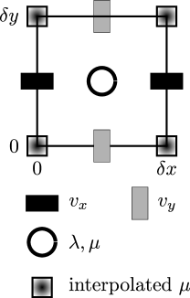
We discretize the equations on a staggered grid, with the displacement located at cell faces as shown in Figure 1. Our method requires the shear modulus () at both the cell centers and cell corners. Since is a given function of space, we could compute it exactly at both cell centers and corners. We have found that we get larger reductions in the residuals for each multigrid V-cycle by using the given function to compute the cell centers, and then using the geometric mean to fill the value at the cell corners. Specifically, in 2D, for a reference cell where the bottom left corner is located at , , at that corner is
| (3) |
The subscripts indicate the variable located at an offset of , from the bottom left corner. So is the bottom left corner, is the left face, and is the cell center.
The Lame parameter is only needed at cell centers, so there is no extra interpolation step.
We can specify and one of two ways: analytic expressions and tables. We use the muparser library [11] to evaluate analytic expressions. To compute the modulus at the boundary, we may need the modulus at a point outside the boundary. For analytic expressions, we evaluate the expression at that outside point. For moduli given by a table, we choose the closest point covered by the table.
For multigrid, the modulus on coarser levels is interpolated from finer levels, not directly computed. Using the interpolated values rather than the directly computed values results in larger reductions in the residuals for each multigrid V-cycle. The interpolation onto the cell centered modulus is a simple arithmetic average of all of the fine points in the coarse cell.
This treatment of the modulus works well for the moderate jumps in material properties seen in realistic models of earthquake regions. More extreme jumps would require a more sophisticated treatment, such as applying IIM to material interfaces as well as faults.
2.3 Gauss-Seidel Relaxation
The core of the solver is a red-black Gauss-Seidel relaxation. We first define the residual as the non-zero remnant of equation 1
| (4) |
We discretize the residual in the usual way with centered differences. To be explicit, in 2D, we write the component as
where, in the reference cell
| (5) | ||||
| (6) | ||||
and
We then define the expression as the derivative of the finite difference expression of with respect to . For example, the derivative of is
The Gauss-Seidel update is then given by
| (7) |
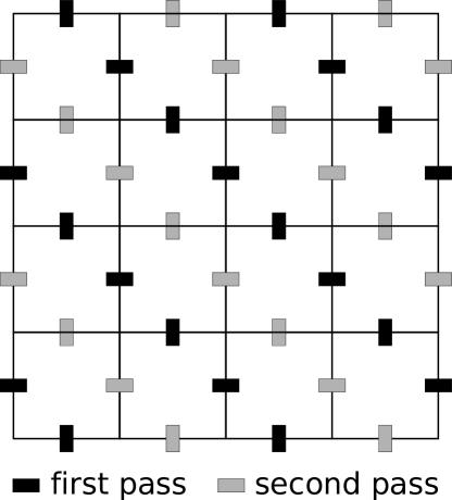
We perform the update in-place in two separate passes as seen in Figure 2. Our discretisation allows us to update each point within a pass independently of each other. Parallelizing the method involves partitioning the mesh into regions that each belong to a different processor. Synchronization only happens before each pass, where each region gets updates to a single layer of ghost zones.
2.4 Treatment of Internal Dislocations
2.4.1 Theory
We define faults as a finite-sized internal surfaces where there is a displacement discontinuity called slip. Fault slip is often described in piece-wise fault segments where displacement is uniform [47, 48, 62, 42, 6, 24, 46], and we follow this convention. This means that a model of a realistic fault will be made up of hundreds of fault segments, each with their own slip. Internal dislocations can cause stress and displacement singularities at the edges of these segments [50, 59, 13]. These singularities do not manifest themselves in real earthquakes because the rock behaves nonlinearly beyond a certain stress by, for example, breaking. However, the nonlinear behavior occurs over a length scale that is orders of magnitude smaller than the rest of the model. So the stress can still get quite high, and these stress concentrations are key to understanding localized deformation. So modeling algorithms must not break down in the presence of these singularities.
To illustrate the method, consider the single faults in 2D in Figure 3. The slip on the faults is given as an input to the problem. To compute at point , we would ordinarily write the finite difference expression
If is constant on each side , then the slip is the difference between them . The finite difference then becomes
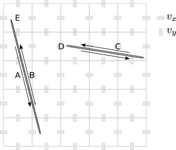
This goes to infinity as the resolution improves and decreases. However, the true value of at that point is zero because is constant. The core idea of the original IIM paper [38] is to model these discontinuities explicitly. Then we compute corrections to apply when computing derivatives. In this case, we can compute the correct derivative by carefully subtracting away the divergent term . Then the corrected expression is
One important note is that this correction is only applied if the line between and crosses the fault. If it barely misses the fault as in the case at point E in Figure 3, there is no correction. This is a significant difference from other methods such as extended finite elements, which can have difficulties arising from small cell volumes or bad aspect ratios [15]. This also implies that the tip of the fault, as seen by these corrections, is only determined up to .
When looking at terms with second derivatives, we build them out of first derivatives. Since the slip is constant along the fault element, there is no correction in the derivatives, only in the displacements. This means that we can build , the correction for , out of , the corrections for . In the reference cell, this is
| (8) |
To be concrete, when applying this method to Eq. 5, the correction at point B in Figure 3 is
| (9) |
The correction to Eq. 6 at point C is
which is zero if the modulus is constant. In contrast, the correction at point D, near the tip of the fault, is
because only the derivative
crosses the fault. Finally, the correction to Eq. 6 at point B is zero because each individual correction is zero.
Note that these corrections do not depend on the type of slip on the fault. For example, if the slip has a tensile opening component, the corrections would have the same form. The only restriction is that the two sides of the fault must be in contact. With that said, we have only tested slip along the faults, so we can only speak with certainty about that kind of slip, referred to as mode II and III in fracture mechanics.
Excluding the tips, these corrections are exact for the type of slip being modeled. This means that the stress is consistent and well behaved across the fault. We might also expect that it would lead to a scheme that converges as . However, the method’s uncertainty about the location of the tips introduces a global error that converges as . At the fault tips themselves, the logarithmic singularity introduces a local error that does not converge.
The above treatment describes a single fault. Since the problem is linear, we can handle multiple faults, each made up of multiple fault segments, by adding all of the corrections from individual fault segments together. This includes the cases where fault segments intersect.
2.4.2 Implementation
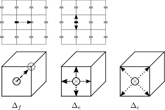
These corrections do not depend on the computed displacement field. In that sense, they could be interpreted as body forces in equation 1. In 3D, this would only require 3 additional numbers per cell. However, that analogy breaks down when we consider the corrections needed when interpolating between coarse and fine levels for multigrid (Section 2.6). With that in mind, we precompute and store the jump in several different directions as shown in Figure 4. In 2D, we store the jump across a cell () and the jump to the corner (). Then, for example, the correction in Eq. 9 becomes
In 2D, this requires storing
extra numbers per cell in addition to the 6 (, , , , , ) already needed. In 3D, we store the jump across the cell (), from the cell face to the edge (), and from the cell face to the corner (). This requires
extra numbers per cell in addition to the 9 already needed.
2.5 Boundary Conditions
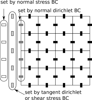
We have implemented two different kinds of boundary conditions: Dirichlet, where the displacement is fixed to a certain value at the boundary, and stress, where the displacement is set so as to dictate what the stress is at a point. When imposing these conditions, it turns out that there is an ordering dependency among the conditions. We must first impose Dirichlet conditions. Then the shear stress conditions use values that were just set by the Dirichlet conditions. Finally, the normal stress conditions use values that were just set by the Dirichlet and shear stress conditions.
2.5.1 Dirichlet
The simplest boundary condition is Dirichlet conditions on the displacement normal to the boundary, as shown in Figure 5. In this case, the value at the boundary is simply set to the boundary value:
For Dirichlet conditions on the displacement tangential to the boundary, as shown in Figure 5, the point outside is set so that the average of the inner and outer points equal to the boundary value:
The correction is necessary to handle any faults between and . For simplicity, we define the faults to never extend out of the mesh.
2.5.2 Stress
A more complicated boundary condition is to set the stress rather than directly setting the displacement.
Shear Stress
The component of the shear stress at an boundary is
We apply this condition by setting at an outside point
This depends on and , so the normal Dirichlet condition must be applied before this condition.
Normal Stress
For the normal stress in the direction in 2D, the analytic condition is , which implies
We discretize this condition as
This interpolates the derivative onto . The moduli, and , are also interpolated there with the usual formula
The condition in 3D has an additional term, , which is computed in a similar manner. This discretization depends on , so the shear stress condition must be applied before this condition.
2.6 Multigrid on an Adapted Mesh
With a smoother (Section 2.3), corrections for faults (Section 2.4), and boundary conditons (Section 2.5), we can compute highly accurate solutions to Eq. 1 on a single grid. This will, however, be very slow. To shorten the time to solution, we implement adaptive multigrid (Appendix A). This is essentially an enhancement of the multigrid method for adapted grids. To implement this, we must first implement coarsening, refinement, and coarse-fine boundary operators.
2.6.1 Coarsening
Following Albers [2] we use weighted arithmetic averages to coarsen the face centered displacement and residuals. Figure 6 shows the fine values used to compute the coarse value for . The corresponding expression in the reference cell is

The expression in 3D is a straightforward extension
At physical boundaries where not all of the values are available, we average only over the face. In 2D, the expression is
and in 3D it is
2.6.2 Refinement
To refine the face-centered variables, we use the stencil shown in Figure 7. We first compute a derivative of the coarse values, which in 2D is

We only refine corrections to the displacement, not the displacement itself. So there is no need to add fault corrections. If we are at the boundary where one of the variables is not available, we use a one-sided derivative. For example, at , the expression is
The fine value is computed from the closest coarse value and this computed derivative
In 3D, the expressions look very similar although now we interpolate along diagonals. For a fine variable on a coarse face, the derivative is
and the fine value is
For fine variables in between coarse faces, we average the fine values on each coarse face:
2.6.3 Coarse-Fine Boundaries
At the interface between coarse and fine levels, we need to compute boundary conditions for the fine mesh given the coarse surrounding mesh. There are two cases of coarse-fine boundaries: vector normal to the interface (e.g., at an x=constant boundary), and vector tangent to the interface (e.g., at a y=constant boundary). When computing these internal boundary conditions, we must use at least quadratic interpolation to keep the overall error second order [40].
Vector Normal to the Interface
Figure 8 shows the stencil that is used to compute the fine boundary value on the coarse-fine interface for the component of a vector that is normal to the interface. The first step is to interpolate the coarse values to the point C. First, we define some variables
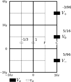
| (10) |
where are the corrections on the coarse grid. Then the coarse value at C is
| (11) |
The final step is to interpolate along a line to get the fine value at F
| (12) | |||||
In 3D, the interpolation for coarse values is along diagonal directions as shown in Figure 9. That means that we can replace Eq. 10 with
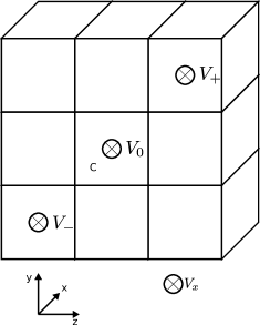
| (13) |
and then use Eq. 11 as is. Eq. 12 is only slightly modified for 3D
| (14) | ||||
If one of the coarse points is outside the physical domain, then we use a simpler interpolation. If is outside, then
and if is outside then
Eq. 14 is used unchanged.
Vector Tangent to the Interface
Figure 10 shows the stencil used for refinement in 2D when the vector is tangential to the interface. For the case where the coarse and fine values are on the same coordinate axis, the interpolation is
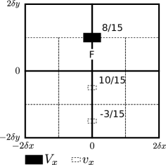
| (15) | ||||
When the fine value does not lie along the coarse grid, we use a simple average of the neighboring coarse values
and the interpolation becomes
At the or corner, some of the fine corrections (e.g. ) are not necessarily defined. For the boundary, we work around this by correcting the coarse value at to first, and then using the same correction from to . With this, the interpolation becomes
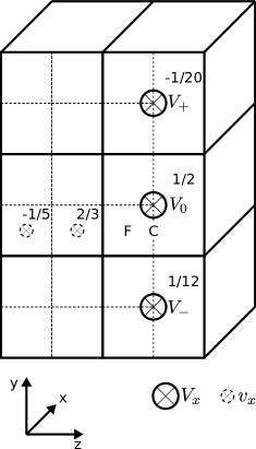
Figure 11 shows the points used for refinement in 3D when the coarse and fine values are on the same coordinate axis. Defining
2.7 Generating the Adapted Mesh
The final part of the method is generating a mesh. Starting with a uniform grid at the coarsest resolution
-
1.
Compute a solution on the current set of grids (section 2.6).
-
2.
If the current number of levels is less than the maximum number of levels
-
(a)
Compute the maximum curvature at each cell center . The curvature in the direction with fault corrections is
At the boundaries, not all points are defined. For example, at an Dirichlet boundary, may not be defined. In these cases, we use a one-sided curvature
We then compute the maximum curvature
-
(b)
Refine all cells where , where is a fixed number, unless the maximum number of mesh refinements has been reached. Note that is an absolute rather than a relative error.
-
(c)
Recurse back to step 1 with the new set of grids.
-
(a)
At fault tips, the displacement is singular and so can never be adequately resolved. However, at a finite distance from the singularity, AMR solutions can still converge [4].
2.8 Accuracy
When solving equation 1 in the presence of faults, there will always be inaccuracies because of the singularities at the tips of the faults. Away from the singularity, we expect convergence (Section 2.4.1). At the singularity, analysis becomes difficult because the Taylor series approximation breaks down. However, the scheme in Section 2.7 monitors this error and refines where needed. This means that, where the algorithm has stopped refining, the discretization error should be less than the error bound . In practice, the actual error will be larger because the local error gets integrated along the points from the boundaries and singularities.
An additional source of error arises because we only approximately solve equation 1. If there is an error in the displacement , that will generate an error in the derivative of approximately , where is the grid spacing. This implies that, for a given , the error in the stress will be at least
where is the smallest value of or . The modulus does not, in our problem, vary wildly, so . This implies that the error in the divergence of the stress is approximately
Using equation 4, we relate this to the size of the residual
Errors in do not contribute to errors in , so that term can be neglected. Simplifying this gives an estimate for the size of the error in terms of the residual
This error will become comparable to the discretization error when , so we can turn this around to find the minimum resolution required to ensure that the solver error is smaller than the discretization error
| (16) |
To be clear, this analysis only covers errors in solving 1 using fault segments. We do not claim to model all of the physical effects (e.g. non-linear rheologies, topography, curved faults).
3 Analytic Tests
We have implemented this method in the parallel, adaptive code Gamra. Gamra uses the SAMRAI framework [29, 30] to handle the bookkeeping associated with multiple levels, multiple grids, and multiple parallel processes. SAMRAI is a mature, freely available, actively developed framework for large-scale parallel structured adaptive mesh refinement. SAMRAI uses MPI to coordinate work among the different processors. This has allowed us to run Gamra on a wide variety of parallel architectures: SMP nodes, traditional Linux clusters, a Blue Gene /Q, and the Intel Xeon Phi 5110p GPGPU.
In this section we perform a number of tests to ensure that the algorithm works as expected and that we implemented it correctly. We have verified that the code works in both 2D and 3D, but mostly discuss the 3D results for brevity. The tests are available from the Gamra repository111https://bitbucket.org/wlandry/gamra, changeset 679:c8843527b10f18758e58011c57d5aa61098c88e2, directory input/benchmarks/Elastic.
3.1 Expanding Cylinder in a Heterogeneous Medium
This is a simple test to ensure that we handle variable elastic modulus correctly. In cylindrical symmetry, if we set the moduli and body forces to
then the basis functions for solutions to Eq. 1 which are purely cylindrical with no rotation or vertical components are
| (17) |
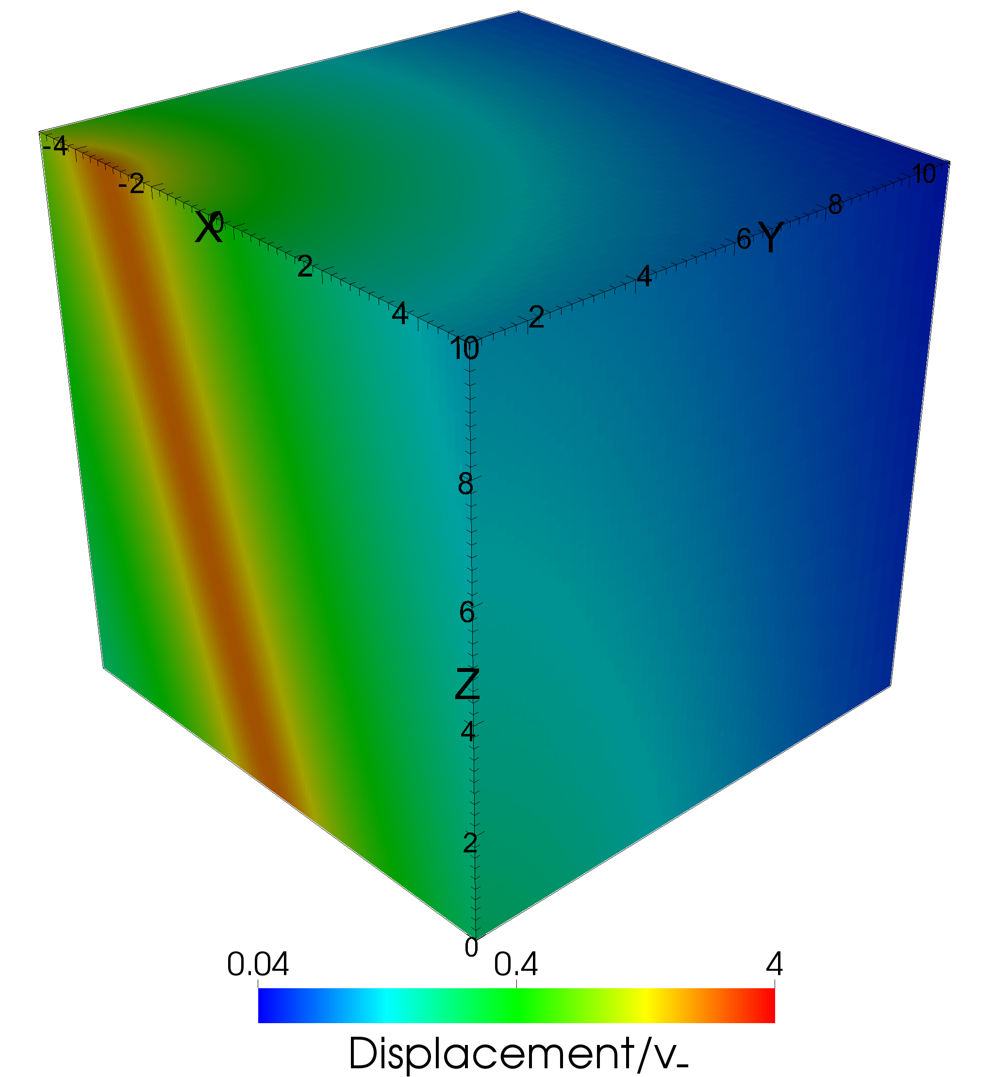
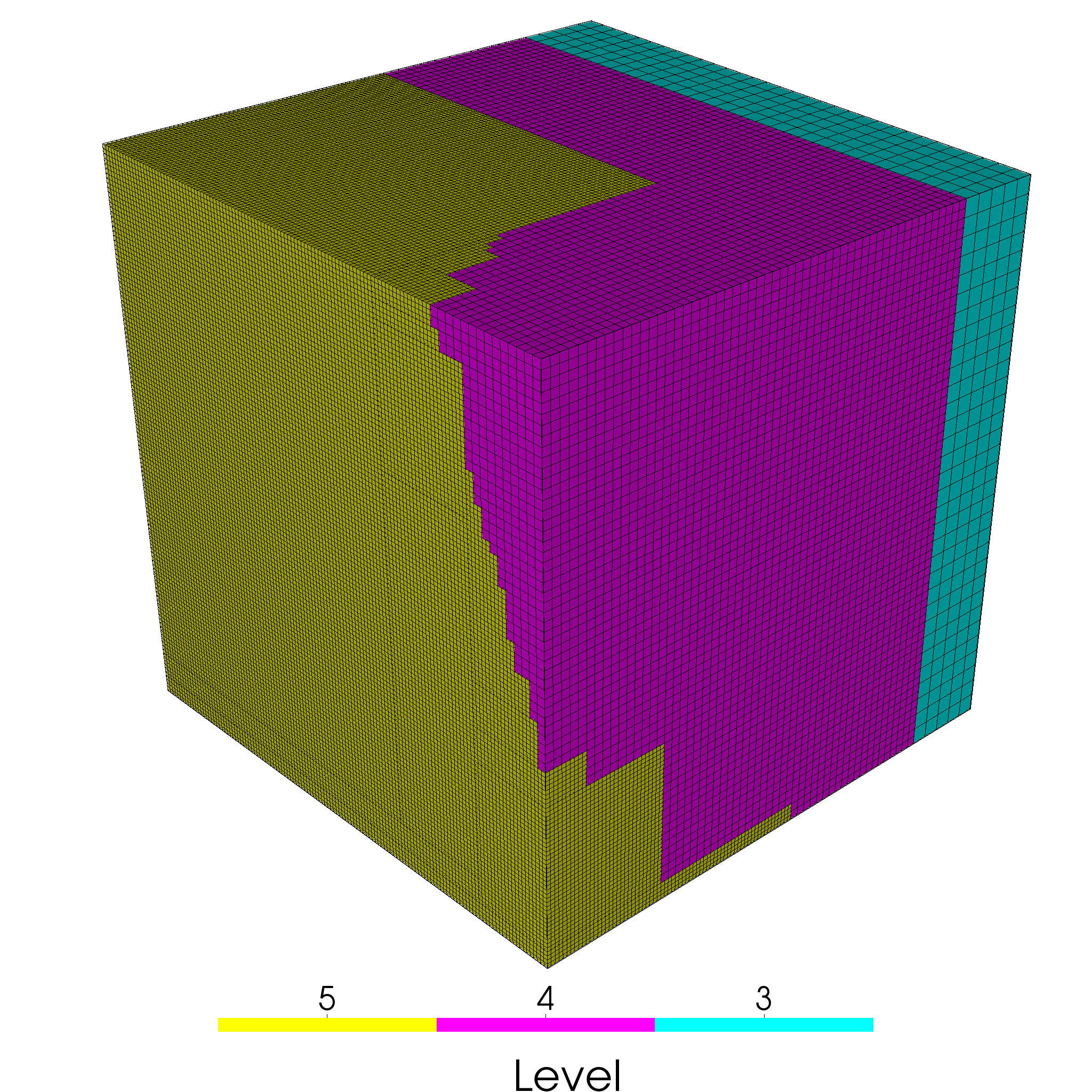
To make the test more rigorous, we rotate the solution by an angle around the axis. Figure 12 shows a numerical solution and its associated adapted grid for a model with , , , and . Table 1 shows the , , and error in . While the and errors do converge, they do not converge as . The error in the unrefined regions no longer decreases, because the mesh does not get smaller there. The integral of these small errors over the large unrefined volume is large enough to affect the overall convergence rate. This is in contrast to the error, which converges uniformly at the expected rate.
| Level | ||||
|---|---|---|---|---|
| 0 | 58.1 | 5.10 | 0.859 | |
| 1 | 5.86 | 0.612 | 0.168 | 5.11 |
| 2 | 1.36 | 0.125 | 0.0409 | 4.11 |
| 3 | 0.344 | 0.0313 | 0.0118 | 3.48 |
| 4 | 0.0819 | 7.79e-3 | 3.13e-3 | 3.76 |
| 5 | 0.0378 | 2.33e-3 | 8.02e-4 | 3.90 |
3.2 Internal dislocations
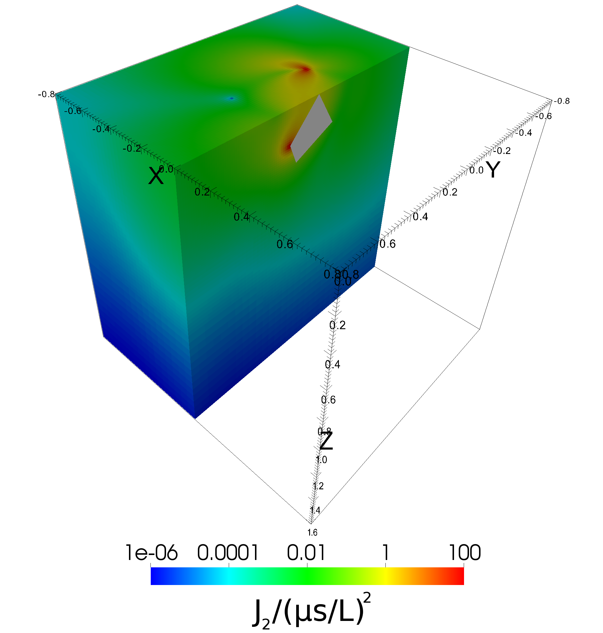
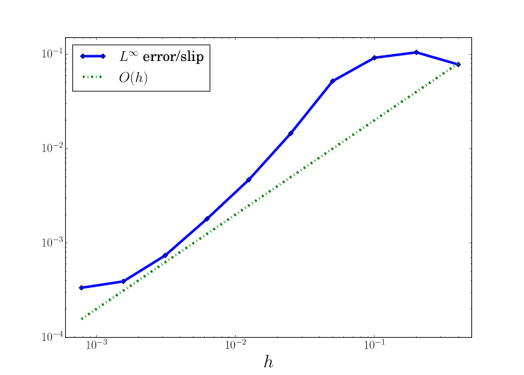
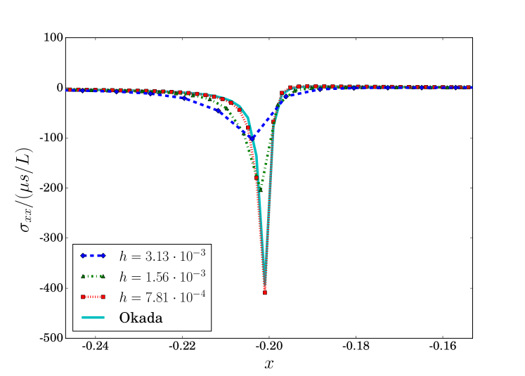
Okada [47, 48] derived an analytic expression for the displacement due to a single fault in a homogeneous elastic half space. Figure 13 shows a solution computed by Gamra for an inclined, rotated fault. As the grid size gets more refined, the mesh places points closer and closer to the singularity. This means that the global error does not shrink, but rather grows with finer resolution. To get around this, we cut holes around the singularities and compute the error on that region. Figure 14 shows the error as a function of resolution. We see that the error scales as up to the point where the error becomes comparable to the criteria for adapting the mesh. Moreover, Figure 15 shows that, for a line crossing near the singularity in the displacement, the stress is well behaved.
We have also run tests where we replace one of the normal Dirichlet conditions (Section 2.5.1) with a normal stress boundary condition (Section 2.5.2) set using the exact Okada stress. Similarly, we ran tests which replaced one of the shear stress conditions (Section 2.5.2) with a tangential Dirichlet condition (Section 2.5.1). All of these tests converge in a similar manner.
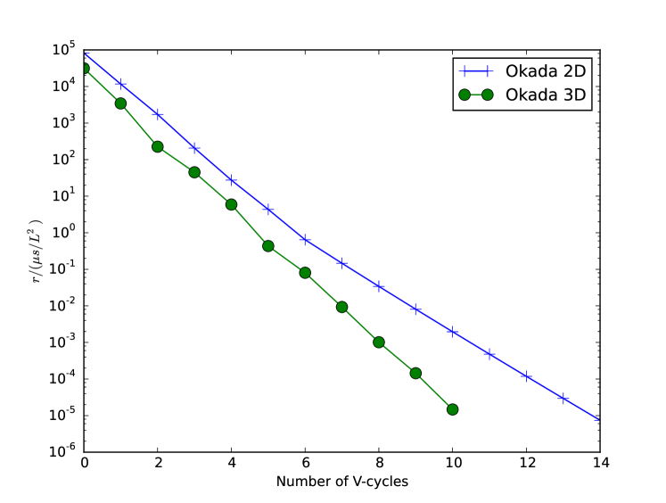
Figure 16 shows the residual versus the number of multigrid V-cycles for 2D and 3D. In spite of the singularity at the fault tips, the solvers perform well, with the per-iteration reduction of the residual tending asymptotically to about 0.25 in 2D and 0.12 in 3D. The 3D solver uses 4 rather than 2 sweeps per multigrid level, so the absolute reduction in the residual is larger.
This gives us some confidence that all of the moving parts involved in computing the solution: smoothing (Section 2.3), boundary conditions (Section 2.5), multigrid (Section 2.6), and adaptivity (Section 2.7) are correct and implemented correctly.
4 1992 Mw 7.3 Landers earthquake
4.1 Setup
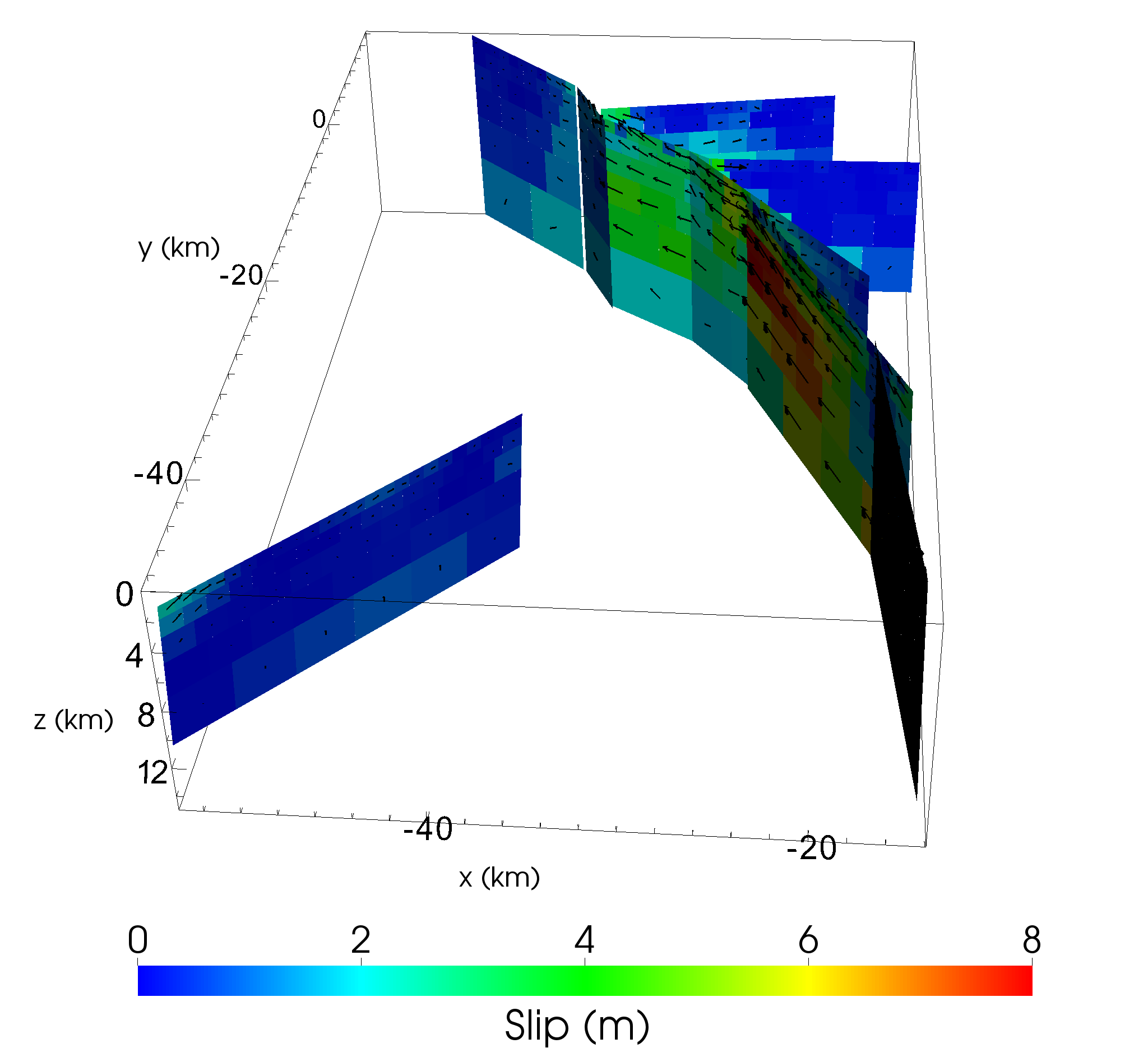
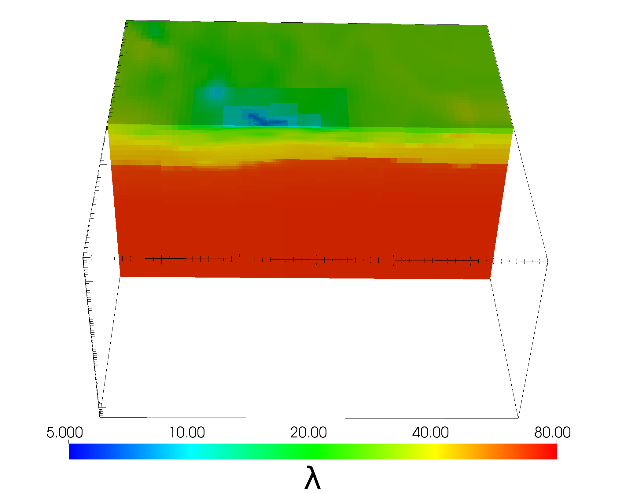
We construct a realistic model of the 1992 Mw 7.3 Landers earthquake using the slip model from Fialko [23] and the material model from the Southern California Earthquake Center Community Velocity Model - Harvard (CVM-H) [60]. The slip model consists of 426 individual fault segments (Figure 17). Figure 17 also shows the variation of Lame’s first parameter, . The second Lame parameter, , has similar structure.
The boundaries are about 100-200 km away from the faults. The boundary conditions on the sides and bottom are free slip: zero shear stress (Section 2.5.2) and zero normal displacement (Section 2.5.1). The boundary condition on the top is free surface: zero shear and normal stress (Section 2.5.2). Since these boundary conditions are imperfect, the error due to the boundaries is about the size of the displacement at the boundary: 1 cm. Getting the error down to the current limits of GPS technology (about 0.5 mm [27, 36, 63]), would require moving the boundaries so far away such that other effects not accounted for (e.g. topography, curvature of the earth) would become significant.
During a multigrid V-cycle, we used 4 pre- and post- sweeps. On the coarsest level, we smoothed 32 times to get an approximate solution. We set the refinement criteria (Section 2.7) to our estimate of the boundary error: 1 cm. We continue multigrid V-cycles until the norm of the residual (Eq. 4) is less than . From equation 16, this implies a minimum resolution of , which in this case is satisfied when the refinement level is at least 3. The mesh is globally refined to level 3, so the error is always dominated by the discretization.
4.2 Results
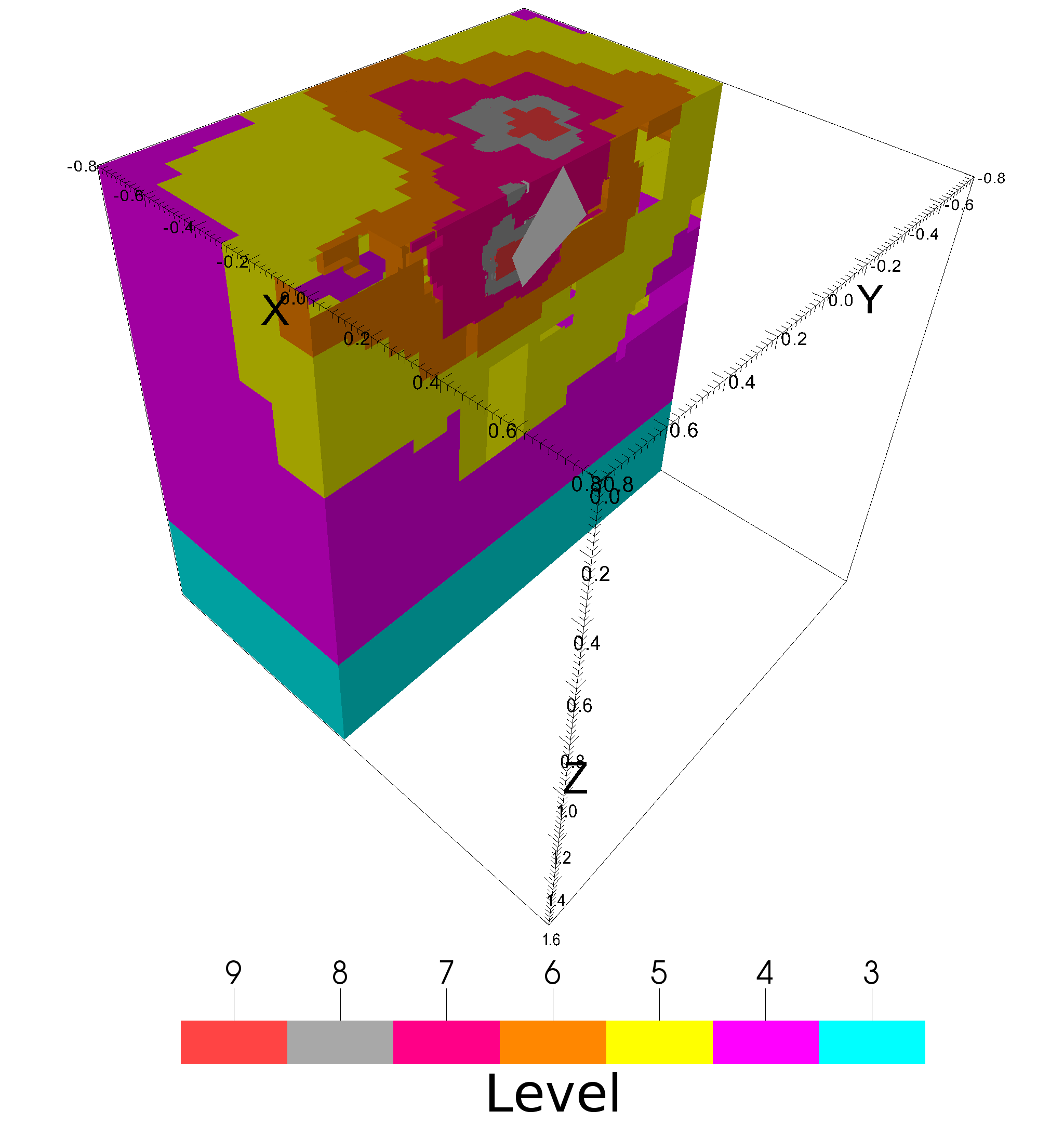
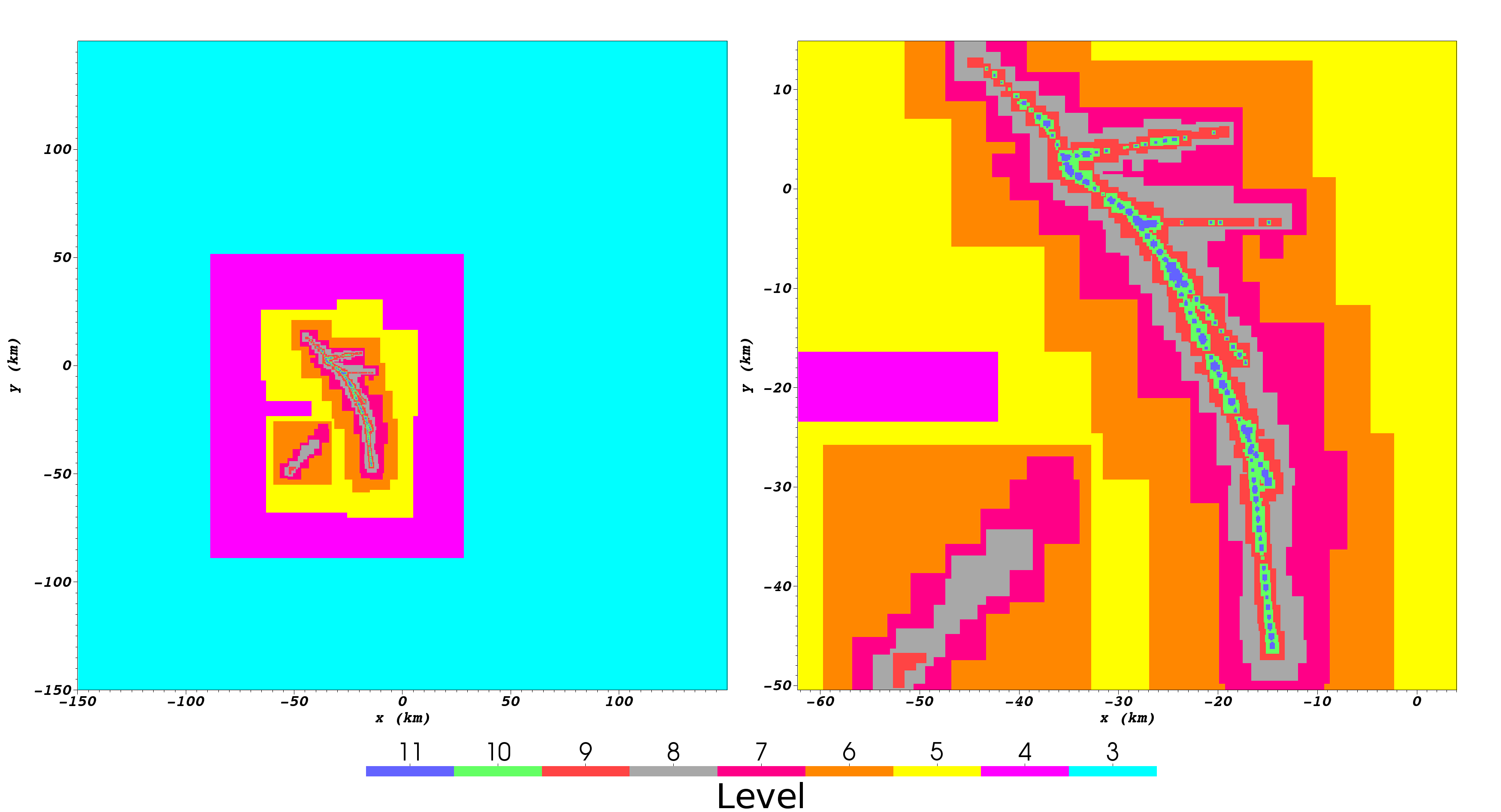
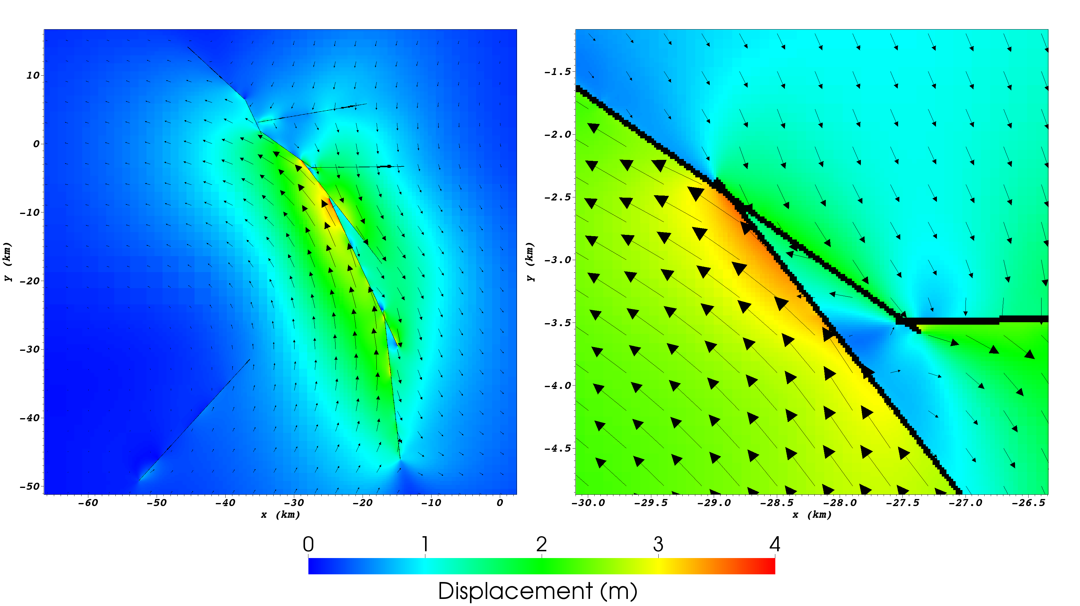
Gamra automatically generated the highly adapted mesh in Figure 18. This mesh has elements, while an equivalent non-adaptive mesh would require elements. The computed solution in Figure 19 highlights the discontinuous nature of the solutions. We expect the error to be concentrated close to the faults, as in Figure 14. So even though the error may be larger near the faults, this would not translate to a large offset error farther from the faults. With that in mind, we expect that the error in displacement in the regions covered by levels 3-10 to be about 1 cm, or about 0.125% of the maximum displacement. Otherwise, the automatic refinement criteria would have marked those regions for refinement.
4.3 Performance
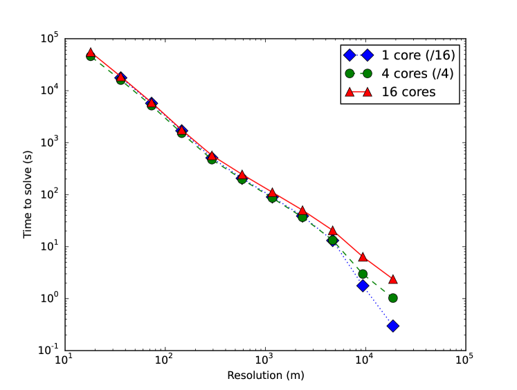
We computed this Landers earthquake solution on a Xen virtual machine running in a Dell R720 with 16 physical cores (Intel Xeon CPU E5-2670) and 256 GB of RAM using OpenMPI 1.8.8 and gcc 4.7.3. Figure 20 shows the time to solve as a function of resolution and number of cores. Altogether, the scaling is quite good at finer resolutions on this shared memory architecture.
Although it is difficult to see in the plot, we see superlinear scaling from 1 to 4 cores for finer resolution. This superlinear scaling does not persist for higher core counts. This is probably a quirk due to running inside a virtual machine. On different hardware without a virtual machine (8 physical core Intel Xeon CPU E5620), we do not see superlinear scaling.
We can roughly fit the relation between time and grid spacing on the plot with a power law This is significantly better than a solver on a fixed three-dimensional grid. Even an optimal multigrid solver would scale as .
5 Conclusion
Elastic deformation due to the displacement of faults can be modeled efficiently with parallel multigrid methods using adaptive meshes and embedded interfaces. The multigrid efficiency is commensurate with what is expected for the simpler Poisson’s equation multigrid solvers [61], in spite of the added complexity brought by internal dislocations and mixed boundary conditions. The computational efficiency is improved by the mesh adaptivity, which reduces the number of nodes by orders of magnitudes compared with uniform meshes. A key advantage of the proposed method is the ability to simulate complex fault geometries without manual and labor-intensive meshing. Even in these complex models, we experienced no problems due to instabilities in the solver or excess sensitivity of the final solution to small changes in the input.
In addition, the method offers high precision in the near field of faults, even capturing the stress singularity asymptotically (Figure 15). This is important for evaluating stress and other dynamic variables. All of these features make the proposed approach optimal for generating stress and displacements kernels for inversions for fault slip [5], investigation of the surrounding elastic structure [8, 14], and building stress and displacement kernels for simulations using the boundary-integral method.
This study presents an important building block of earthquake cycle simulations. A future major undertaking will be to incorporate rupture dynamics and quasi-static off-fault deformation. Fault dynamics will require modeling the propagation of seismic waves. The mesh adaptivity may then be exploited to implement spatially variable adaptive time steps [43]. Quasi-static time-dependent problems with off-fault plasticity and visco-elastic or poro-elastic deformation may be treated with the same elliptic solver using equivalent body forces (per unit time), requiring only more book-keeping to handle explicit time steps. Many other effects may be incorporated to enable even more realistic models of earthquakes and Earth deformation, such as a spherical geometry for global-scale models and topography to improve calculation of local stress.
6 Acknowledgements
We thank two anonymous reviewers for their comments that improved this manuscript. This research used resources of the Argonne Leadership Computing Facility, which is a DOE Office of Science User Facility supported under Contract DE-AC02-06CH11357. This research was supported by the Gordon and Betty Moore Foundation, NSF Award EAR-0949446, the Tectonics Observatory, the National Research Foundation of Singapore under the NRF Fellowship scheme (National Research Fellow Award No. NRF-NRFF2013-04) and by the Earth Observatory of Singapore and the National Research Foundation and the Singapore Ministry of Education under the Research Centres of Excellence initiative. This is EOS publication 113.
Appendix A Adaptive Multigrid
For completeness, we detail the exact adaptive multigrid algorithm we use. This is mostly a restatement of Section 4 of Martin & Cartwright [40].
First, we define a Gauss-Seidel operator , where is an initial guess, is the forcing term, and is the number of times to apply the smoother. The output of is a correction
| (18) |
For , Equation 7 implies
where is defined by Equation 4. Next we define a recursive multigrid V-cycle relaxation routine , where is the current level and is the defect. The outline of the routine is as follows.
-
1.
If (the coarsest level)
-
(a)
Using an initial guess of 0, compute a correction by applying the smoother times
or until the norm of the residual is less than .
-
(a)
-
2.
If
-
(a)
Using an initial guess of 0, compute a correction by applying the smoother times
-
(b)
Compute , the residual on just the fine grid (Section 2.3).
-
(c)
Coarsen to make (Section 2.6.1)
-
(d)
Recursively call MGRelax to get the coarse grid correction
-
(e)
Refine the correction to the fine level (Section 2.6.2) and add it to the fine correction
-
(f)
Apply the smoother times to get a final correction
-
(a)
-
3.
Return .
Given these functions, the driver routine is short.
- 1.
-
2.
While the norm of the residual is less than the stopping tolerance
-
(a)
Compute .
-
(b)
Add in the correction
-
(c)
Recompute the composite residual .
-
(a)
In pseudo-code, MGRelax is
-
Procedure :
if :
for (i =0; i<; ++i)
if :
break
else:
return
and the driver is
-
while
References
- [1] B. T. Aagaard, M. G. Knepley, and C. A. Williams. A domain decomposition approach to implementing fault slip in finite-element models of quasi-static and dynamic crustal deformation. J. Geophys. Res., 118(6):3059–3079, 2013.
- [2] M. Albers. A local mesh refinement multigrid method for 3-d convection problems with strongly variable viscosity. J. Comp. Phys., 160:216–150, 2000.
- [3] D. J. Andrews. A fault constitutive relation accounting for thermal pressurization of pore fluid. J. Geophys. Res., 107:10.1029/2002JB001942, 2002.
- [4] D. Bai and A. Brandt. Local mesh refinement multilevel techniques. J. Sci. Stat. Comput., 8(2):109–134, 1987.
- [5] S. Barbot, P. Agram, and M. De Michele. Change of Apparent Segmentation of the San Andreas Fault Around Parkfield from Space Geodetic Observations Across Multiple Periods. J. Geophys. Res., 118(12):6311–6327, 2013.
- [6] S. Barbot and Y. Fialko. Fourier-domain Green’s function for an elastic semi-infinite solid under gravity, with applications to earthquake and volcano deformation. Geophys. J. Int., 182(2):568–582, 2010.
- [7] S. Barbot and Y. Fialko. A unified continuum representation of postseismic relaxation mechanisms: semi-analytic models of afterslip, poroelastic rebound and viscoelastic flow. Geophys. J. Int., 182(3):1124–1140, 2010.
- [8] S. Barbot, Y. Fialko, and D. Sandwell. Three-Dimensional Models of Elasto-Static Deformation in Heterogeneous Media, with Applications to the Eastern California Shear Zone. Geophys. J. Int., 179(1):500–520, 2009.
- [9] S. Barbot, N. Lapusta, and J. P. Avouac. Under the hood of the earthquake machine: Towards predictive modeling of the seismic cycle. Science, 336(6082):707–710, 2012.
- [10] R. Becker, E. Burman, and P. Hansbo. A nitsche extended finite element method for incompressible elasticity with discontinuous modulus of elasticity. Computer Methods in Applied Mechanics and Engineering, 198(41):3352–3360, 2009.
- [11] I. Berg. muparser home page. http://muparser.beltoforion.de/, 2014.
- [12] O. Botella and Y. Cheny. The ls-stag method for viscous incompressible flows in irregular geometries: Basics of the discretization and application to viscoelastic flows. In ASME 2010 3rd Joint US-European Fluids Engineering Summer Meeting collocated with 8th International Conference on Nanochannels, Microchannels, and Minichannels, pages 2441–2451. American Society of Mechanical Engineers, 2010.
- [13] R. Bürgmann, D. D. Pollard, and S. J. Martel. Slip distributions on faults: effects of stress gradients, inelastic deformation, heterogeneous host-rock stiffness, and fault interaction. Journal of Structural Geology, 16(12):1675–1690, 1994.
- [14] Y. Cochran, Y.-G. Li, P. Shearer, S. Barbot, Y. Fialko, and J. Vidale. Seismic and geodetic evidence for extensive, long-lived fault damage zones. Geology, 37(4):315–318, Apr. 2009.
- [15] E. T. Coon, B. E. Shaw, and M. Spiegelman. A nitsche-extended finite element method for earthquake rupture on complex fault systems. Comput. Methods Appl. Mech. Engrg., 200:2859–2870, 2011.
- [16] Y. Cui, K. B. Olsen, T. H. Jordan, K. Lee, J. Zhou, P. Small, D. Roten, G. Ely, D. K. Panda, A. Chourasia, et al. Scalable earthquake simulation on petascale supercomputers. In Proc. 2010 ACM/IEEE Int. Conf. High Perf. Comp., Net., Storage Analysis, pages 1–20. IEEE Computer Society, 2010.
- [17] S. M. Day. Three-dimensional finite difference simulation of fault dynamics: rectangular faults with fixed rupture velocity. Bull. Seism. Soc. Am., 72(3):705–727, 1982.
- [18] S. M. Day, L. A. Dalguer, N. Lapusta, and Y. Liu. Comparison of finite difference and boundary integral solutions to three-dimensional spontaneous rupture. J. Geophys. Res., 110(B12307), 2005.
- [19] E. M. Dunham and R. J. Archuleta. Near-source ground motion from steady state dynamic rupture pulses. Geophys. Res. Lett., 32(3), 2005.
- [20] E. M. Dunham, J. E. Kozdon, D. Belander, and L. Cong. Earthquake ruptures on rough faults. In Multiscale and multiphysics processes in geomechanics: Results of the workshop on Multiscale and multiphysics processes in geomechanics, Stanford, June 23-25, 2010, page 145. Springer Science & Business Media, 2011.
- [21] G. P. Ely, S. M. Day, and J.-B. Minster. A support-operator method for 3-d rupture dynamics. Geophys. J. Int., 177(3):1140–1150, 2009.
- [22] G. P. Ely, S. M. Day, and J.-B. Minster. Dynamic rupture models for the southern san andreas fault. Bull. Seism. Soc. Am., 100(1):131–150, 2010.
- [23] Y. Fialko. Probing the mechanical properties of seismically active crust with space geodesy: Study of the co-seismic deformation due to the 1992 M Landers (Southern California) earthquake. J. Geophys. Res., 109(B03307), 2004.
- [24] Z. Gimbutas, L. Greengard, M. Barall, and T. E. Tullis. On the calculation of displacement, stress, and strain induced by triangular dislocations. Bull. Seism. Soc. Am., 102(6):2776–2780, 2012.
- [25] R. A. Harris, M. Barall, R. Archuleta, E. Dunham, B. Aagaard, J.-P. Ampuero, D. J. Andrews, H. Bhat, V. Cruz-Atienza, L. Dalguer, S. Day, B. Duan, G. Ely, Y. Kaneko, Y. Kase, N. Lapusta, Y. Liu, S. Ma, D. Oglesby, K. Olsen, A. Pitarka, S. Song, and E. Templeton. The SCEC/USGS Dynamic Earthquake Rupture Code Verification Exercise. Seism. Res. Lett., 80(1):119–126, 2009.
- [26] R. Hassani, D. Jongmans, and J. Chéry. Study of plate deformation and stress in subduction processes using two-dimensional numerical models. J. G. R., 102(B8):17951–17965, 1997.
- [27] E. M. Hill, J. L. Davis, P. Elòsegui, B. P. Wernicke, E. Malikowski, and N. A. Niemi. Characterization of site-specific gps errors using a short-baseline network of braced monuments at yucca mountain, southern nevada. J. Geophys. Res., 114(B11402):13, 2009.
- [28] T. Hori, N. Kato, K. Hirahara, T. Baba, and Y. Kaneda. A numerical simulation of earthquake cycles along the Nankai Trough in southwest Japan: lateral variation in frictional property due to the slab geometry controls the nucleation position. Earth Plan. Sci. Lett., 228(3-4):215–226, 2004.
- [29] R. D. Hornung and S. R. Kohn. Managing application complexity in the samrai object-oriented framework. Concurrency and computation: practice and experience, 14:347–368, 2002.
- [30] R. D. Hornung, A. M. Wissink, and S. R. Kohn. Managing complex data and geometry in parallel structured amr applications. Engineering with Computers, 2006.
- [31] Y. Kaneko, J.-P. Ampuero, and N. Lapusta. Spectral-element simulations of long-term fault slip: Effect of low-rigidity layers on earthquake-cycle dynamics. J. Geophys. Res., 116(B10313), 2011.
- [32] Y. Kaneko, J.-P. Avouac, and N. Lapusta. Towards inferring earthquake patterns from geodetic observations of interseismic coupling. Nature Geoscience, 3:363–369, 2010.
- [33] Y. Kaneko, N. Lapusta, and J.-P. Ampuero. Spectral element modeling of spontaneous earthquake rupture on rate and state faults: Effect of velocity-strengthening friction at shallow depths. J. Geophys. Res., 113:17, 2008.
- [34] N. Kato. Interaction of slip on asperities: Numerical simulation of seismic cycles on a two-dimensional planar fault with nonuniform frictional property. J. Geophys. Res., 109, 2004.
- [35] J. Kozdon, E. M. Dunham, and J. Nordström. Simulations of dynamic earthquake ruptures in complex geometries using high-order finite difference methods. J. Sci. Comput., 55:92–124, 2013.
- [36] J. Langbein. Noise in GPS displacement measurements from Southern California and Southern Nevada. J. Geophys. Res., 113(B05405), 2008.
- [37] N. Lapusta and S. Barbot. Models of earthquakes and aseismic slip based on laboratory-derived rate and state friction laws. In A. Bizzarri and H. S. Bhat, editors, The mechanics of Faulting: From Laboratory to Real Earthquakes. 2012.
- [38] R. J. Leveque and Z. Li. The immersed interface method for elliptic equations with discontinuous coefficients and singular sources. SIAM J. Numer. Anal., 31(4):1019–1044, 1994.
- [39] S. T. Marshall, M. L. Cooke, and S. E. Owen. Effects of nonplanar fault topology and mechanical interaction on fault-slip distributions in the ventura basin, california. Bull. Seism. Soc. Am., 98(3):1113–1127, 2008.
- [40] D. F. Martin and K. L. Cartwright. Solving Poisson’s equation using adaptive mesh refinement. Electronics Research Laboratory, College of Engineering, University of California, 1996.
- [41] T. Matsuzawa, H. Hirose, B. Shibazaki, and K. Obara. Modeling short- and long-term slow slip events in the seismic cycles of large subduction earthquakes. J. Geophys. Res., 115(B12301), 2010.
- [42] B. J. Meade. Algorithms for the calculation of exact displacements, strains, and stresses for triangular dislocation elements in a uniform elastic half space. Comp. Geosc., 33(8):1064–1075, Aug. 2007.
- [43] Z. Meglicki, S. K. Gray, and B. Norris. Multigrid fdtd with chombo. Computer physics communications, 176(2):109–120, 2007.
- [44] H. J. Melosh and C. A. Williams. Mechanics of graben formation in crustal rocks: a finite element analysis. J. Geophys. Res., 94(B10):13961–13973, 1989.
- [45] P. Moczo, J. Kristek, and M. Gális. The Finite-Difference Modelling of Earth Quake Motions: Waves and Ruptures. Cambridge University Press, 2014.
- [46] M. Nikkhoo and T. R. Walter. Triangular dislocation: an analytical, artefact-free solution. Geophysical Journal International, 201(2):1117–1139, 2015.
- [47] Y. Okada. Surface deformation due to shear and tensile faults in a half-space. Bull. Seism. Soc. Am., 75(4):1135–1154, Aug. 1985.
- [48] Y. Okada. Internal deformation due to shear and tensile faults in a half-space. Bull. Seism. Soc. Am., 82:1018–1040, April 1992.
- [49] K. B. Olsen, R. Madariaga, and R. J. Archuleta. Three-Dimensional Dynamic Simulation of the 1992 Landers Earthquake. Science, 278(5339):834–838, 1997.
- [50] P. C. Paris and G. C. Sih. Stress analysis of cracks. ASTM stp, 381:30–81, 1965.
- [51] J. Puente, J.-P. Ampuero, and M. Käser. Dynamic rupture modeling on unstructured meshes using a discontinuous galerkin method. J. Geophys. Res., 114(B10), 2009.
- [52] J. R. Rice. Spatio-temporal complexity of slip on a fault. J. Geophys. Res., 98(B6):9885–9907, 1993.
- [53] J. C. Rollins, S. Barbot, and J.-P. Avouac. Mechanisms of Postseismic Deformation Following the 2010 El Mayor-Cucapah Earthquake. Pure App. Geophys., page 54, 2015.
- [54] B. Rousset, S. Barbot, J. P. Avouac, and Y.-J. Hsu. Postseismic Deformation Following the 1999 Chi-Chi Earthquake, Taiwan: Implication for Lower-Crust Rheology. J. Geophys. Res., 117(B12405):16, 2012.
- [55] V. Rutka, H. Andrä, and A. Wiegmann. EJIIM for calculation of effective elastic moduli in 3D linear elasticity. ITWM, 2006.
- [56] V. Rutka and A. Wiegmann. Explicit jump immersed interface method for virtual material design of the effective elastic moduli of composite materials. Numerical Algorithms, 43(4):309–330, 2006.
- [57] B. Shibazaki and T. Shimamoto. Modelling of short-interval silent slip events in deeper subduction interfaces considering the frictional properties at the unstablestable transition regime. Geophys. J. Int., 171(1):191–205, 2007.
- [58] B. Smith and D. Sandwell. A three-dimensional semianalytic viscoelastic model for time-dependent analyses of the earthquake cycle. J. Geophys. Res., 109, 2004.
- [59] H. Tada, P. Paris, and G. Irwin. The analysis of cracks handbook. New York: ASME Press, 2000.
- [60] C. Tape, Q. Liu, A. Maggi, and J. Tromp. Adjoint tomography of the southern California crust. Science, 325:988–992, 2009.
- [61] U. Trottenberg, C. W. Oosterlee, and A. Schuller. Multigrid. Academic press, 2000.
- [62] R. Wang, F. Martin, and F. Roth. Computation of deformation induced by earthquakes in a multi-layered elastic crust - FORTRAN programs EDGRN/EDCMP. Comp. Geosci., 29:195–207, 2003.
- [63] S. D. P. Williams, Y. Bock, P. Fang, P. Jamason, R. M. Nikolaidis, L. Prawirodirdjo, M. Miller, and D. J. Johnson. Error Analysis of Continuous GPS Position Time Series. J. Geophys. Res., 109(B03412), 2004.
- [64] M. S. T. Zangmeister. On the Extended Finite Element Method for the Elasto-Plastic Deformation of Heterogeneous Materials. PhD thesis, Zugl.: Kaiserslautern, Technische Universität Kaiserslautern, Diss., 2014, 2015.
- [65] Y. Zhu, Y. Wang, J. Hellrung, A. Cantarero, E. Sifakis, and J. M. Teran. A second-order virtual node algorithm for nearly incompressible linear elasticity in irregular domains. Journal of Computational Physics, 231(21):7092–7117, 2012.