Deterministic and stochastic aspects of the stability in an inverted pendulum under a generalized parametric excitation

Abstract

In this paper, we explore the stability of an inverted pendulum under a generalized parametric excitation described by a superposition of $N$ cosines with different amplitudes and frequencies, based on a simple stability condition that does not require any use of Lyapunov exponent, for example. Our analysis is separated in 3 different cases: $N=1$, $N=2$, and $N$ very large. Our results were obtained via numerical simulations by fourth-order Runge Kutta integration of the non-linear equations. We also calculate the effective potential also for $N>2$. We show then that numerical integrations recover a wider region of stability that are not captured by the (approximated) analytical method. We also analyze stochastic stabilization here: firstly, we look the effects of external noise in the stability diagram by enlarging the variance, and secondly, when $N$ is large, we rescale the amplitude by showing that the diagrams for time survival of the inverted pendulum resembles the exact case for $N=1$. Finally, we find numerically the optimal number of cosines corresponding to the maximal survival probability of the pendulum.

1 Introduction

The inverted pendulum, more precisely its stabilization mechanisms deserve a lot of attention from several correlated areas, including Physics, Mathematics, Biology, (see for example an interesting review [1]). However, the applications goes beyond, including the study of excitation effects in Ocean Structures [2], inverted pendulum robots [3] and many others.

Induced stability is a solved problem known since 1908 [4], but it was in the 1950s, with Kapiza [5], that this kind of stability was studied for the inverted pendulum system. Experimental results were obtained in the 1960s (see for example [6]) and even nowadays this problem still remains interesting [7]. The possible excitations/perturbations which may be capable of stabilizing an inverted pendulum, even for some time, have a large number of details which are not completely understood yet. Therefore, this apparent simple system, has a complexity that can be considered a challenging problem since some important stabilization problems in Engineering, as for instance, the stability of robot arms, the stability of populations in biology [1], or even the stabilization of photons deviation in Cosmology [8] require similar stabilization mechanisms.

An inverted pendulum (showin in Fig. 1) free of external forces, is unstable and the punctual mass $m$ attached to the rigid massless rod will tend to oscillate around to the stable equilibrium position ($\theta=180^{0}$), which corresponds to the usual pendulum problem).

In order to keep the pendulum upright, $\cos\theta>0$, the frictionless hinge that attaches the rod to the suspension point point, must vertically accelerated. Let us denote such acceleration by $a(t)=\ddot{z}(t)$, where $z(t)$ is a time-dependent excitation that controls the height of the pendulum suspension point $P$.

Figure 1: Inverted pendulum under a support excitation $z(t)$.

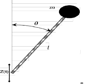
The Lagrangian of this problem can easily be written as:

$$\mathcal{L}(\theta,\dot{\theta})=\frac{1}{2}ml^{2}\dot{\theta}^{2}-ml\dot{z}\dot{\theta}\sin\theta-mgl\cos\theta-mgz(t)\text{.}$$

It is worth emphasizing that all our results can be directly extended to an equivalent physical pendulum making simple associations. If we additionally consider a external excitation $\phi(t)$ we can derive the motion equation

$$\ddot{\theta}(t)=\frac{g}{l}\left(1+\frac{1}{g}\ddot{z}(t)\right)\sin\theta+\phi(t)$$ (1)

from the Lagrange equations.

Now, in order to generalize, we write $z(t)=z_{\text{det}}(t)+z_{\text{rand}}(t)$ and $\phi(t)=\phi_{\text{det}}(t)+\phi_{\text{rand}}(t)$ where subscripts “det” and “rand” denote the deterministic and stochastic time-dependent parts of the excitations/perturbations respectively. In this work, we focus our analysis in two important situations: $z_{\text{rand}}(t)=0$ and $z_{\text{det}}(t)=$ $\sum_{j=1}^{n}A_{j}\cos(\omega_{j}t)$, i.e., parametric sinusoidal excitation in the basis and $\phi_{\text{det}}(t)=0$ and $\phi_{\text{rand}}(t)=N(\mu,\sigma)$ that denotes an external gaussian noise with mean $\mu$ and standard deviation $\sigma$. The more appropriate choice here is $\mu=0$, given that we are mainly interested in the parametric stabilization of the inverted pendulum or in what we can call its survival time $\tau$, which means the maximum time the pendulum remains upright or, mathematically, the time up to condition $\cos\theta<0$ is satisfied. The condition $\mu\neq 0$ leads to a natural biased motion, which is not interesting here. In this work we consider to analyze how the stability condition is broken as function of the external noise dispersion $\sigma$.

Several authors [1, 9] have explored the case $N=1$ using small angles approximation known as the effective potential method. However, even the well known case for one cosine, $N=1$, deserves, in our opinion, some attention and alternative analysis. Therefore, firstly, we checked the literature based on numerical integration methods in order to verify the validity of previous results in the small oscillations regime and the initial conditions dependence, basically, the initial angle dependence. Particularly we also use these numerical integrations to observe the breaking of the stability region predicted by perturbative analysis and by parametric resonance (see Butikov [9]) when the external noise is turned on (i.e., $\phi\neq 0$). In this case we calculate the pendulum survival probability over different time evolutions (i.e, different evolutions corresponding to different seeds). A detailed connection between $N=1$ and $N\rightarrow\infty$ is also explored when the pendulum amplitude grows linearly with time and is also rescaled with the number of cosines set in the parametric excitation.

In the second part of this work we analyze the superposition of two cosines, $N=2$, which as far as we are concerned has not been explored yet. This case is interesting since the period of the composition is not always known so that the perturbative analysis is not able to describe the inverted pendulum stability regions correctly. Given such a problem, we analyze numerically the interesting case where the amplitudes are fixed and the frequencies: $\omega_{1}\$and $\omega_{2}$ are varied. The analytical results obtained via the effective potential method are compared with numerical simulations. We also analyze the effects of an analysis of the stability breakdown considering different external noise dispersion $\sigma$ in the numerical diagrams. Deviations from small oscillations behavior were considered in our analysis.

Finally, for $N>2$, we look for optimization problems on the stability probability considering an ensemble of frequencies and amplitudes. The most remarkable detail in our analysis is the fact a simple choice for the stability criterion as, $\cos\theta>0$, overcomes more laborious methods such as Liapunov exponent or other analysis to check stability conditions. So we organized our papers as it follows: in the next section we describe key points for a perturbative analysis extending our formulation for arbitrary $N$, which is known in literature as effective potential method. In section 3, we briefly show our numerical simulations were developed. Our main results are presented in section 4. Some discussions and conclusions are finally presented in section 5.

2 Perturbative Analysis

We start our perturbative analysis by chosing the perturbative function $z(t)=\sum_{i=1}^{N}A_{i}\cos(\omega_{i}t)$, so that the Eq. 1 becomes

$$\frac{d^{2}\theta}{dt^{2}}=\frac{g}{l}\left(1-\frac{1}{g}\sum_{i=1}^{N}A_{i}\omega_{i}^{2}\cos(\omega_{i}t)\right)\sin\theta$$ (2)

where we set up $\phi(t)=0$ for all $t$.

The last equation can be written in a more elucidative form as

$$\overset{\cdot\cdot}{\theta}\ =-\frac{\partial U}{\partial\theta}+F(\theta)$$ (3)

where $U=\frac{g}{l}\cos\theta$ and $F(\theta)=\frac{\overset{..}{z}(t)}{l}\sin\theta=-\frac{\sin\theta}{l}\sum_{i=1}^{N}A_{i}\omega_{i}^{2}\cos(\omega_{i}t)$. The physical interpretation is straightforward here, given that $U(\theta)$ is the gravitational potential, while $F(\theta)$ is an external force due to vibrations at the pendulum suspension point. In what follows from here, we will adapt the equations obtained by Landau and Lifchitz [11]. A similar analysis was developed by Kapitza (1951) [5].

We start assuming that the solution of Eq. 3 can be separated into two aditive components:

$$\theta(t)=\overline{\theta}(t)+\xi(t)\text{.}$$ (4)

We are considering that the pendulum motion is composed by a non-perturbated path $\overline{\theta}$ plus a noise $\xi$ composed by multiple frequencies $\{\omega_{i}\}_{i=1}^{N}$and amplitudes $\{A_{i}\}_{i=1}^{N}$. Another way to think is that $\overline{\theta}(t)$ has a large amplitude but slow frequency while $\xi(t)$ has small amplitude but fast frequency.

By the Taylor expansions of $U(\theta)$ and $F(\theta)$ around the slow path $\overline{\theta}$, we have:

$$\frac{\partial U}{\partial\theta} = \left.\frac{\partial U}{\partial\theta}\right|_{\theta=\overline{\theta}}+\left.\frac{\partial^{2}U}{\partial\theta^{2}}\right|_{\theta=\overline{\theta}}\xi+\frac{1}{2}\left.\frac{\partial^{3}U}{\partial\theta^{3}}\right|_{\theta=\overline{\theta}}\xi^{2}+...$$ (5)

$$\frac{\partial F}{\partial\theta} = F(\overline{\theta})+\left.\frac{\partial F}{\partial\theta}\right|_{\theta=\overline{\theta}}\xi+\left.\frac{\partial^{2}F}{\partial\theta^{2}}\right|_{\theta=\overline{\theta}}\xi^{2}+...$$

Considering these approximations up to the first order term, we can obtain from Eq. 3 that

$$\overset{\cdot\cdot}{\overline{\theta}}+\overset{\cdot\cdot}{\xi}\ =-\left.\frac{\partial U}{\partial\theta}\right|_{\theta=\overline{\theta}}-\left.\frac{\partial^{2}U}{\partial\theta^{2}}\right|_{\theta=\overline{\theta}}\xi+F(\overline{\theta})+\left.\frac{\partial F}{\partial\theta}\right|_{\theta=\overline{\theta}}\xi$$ (6)

Now it is crucial to consider the nature of motion to distinguish the important terms in Eq. 6. The only candidates associated with the perturbative effects on the right side of this equation are $-\left.\frac{\partial^{2}U}{\partial\theta^{2}}\right|_{\theta=\overline{\theta}}\xi$, $F(\overline{\theta})$, and $\left.\frac{\partial F}{\partial\theta}\right|_{\theta=\overline{\theta}}\xi$. Therefore, given that the terms $-\left.\frac{\partial^{2}U}{\partial\theta^{2}}\right|_{\theta=\overline{\theta}}\xi$ and $\left.\frac{\partial F}{\partial\theta}\right|_{\theta=\overline{\theta}}\xi$ are small when compared with $F(\overline{\theta})$ we have

$$\overset{\cdot\cdot}{\xi}\ =F(\overline{\theta})=-\frac{\sin\overline{\theta}}{l}\sum_{i=1}^{N}A_{i}\omega_{i}^{2}\cos(\omega_{i}t)$$ (7)

By integrating the equation 7 twice with respect to time we obtain

$$\xi(t)=\frac{\sin\overline{\theta}}{l}\sum_{i=1}^{N}A_{i}\cos(\omega_{i}t)+c_{1}t+c_{0}$$

Here, $c_{0}$ and $c_{1}$ are arbitrary constants and must be assumed null given that we want $\xi$ to be an oscillatory term, so that it should not increase as a function of time. This is a constraint that can be imposed as initial condition. For a set $\{\omega_{i}\}_{i=1}^{N}$ the superposition $\sum_{i=1}^{N}A_{i}\cos(\omega_{i}t)$ does not necessarily results in a periodic function. For this to occur, there must be a period $T$, such that: $\omega_{i}T=2n_{i}\pi$ and $\omega_{j}T=2n_{j}\pi$, for every pair $i\neq j=1,...,N$, or simply

$$\omega_{i}/\omega_{j}=n_{i}/n_{j}\text{,}$$ (8)

i.e., the ratio between frequencies must be a rational number where $n_{i}$ and $n_{j}$ are the smallest possible integers, so that, $n_{i}/n_{j}$ is an irreducible fraction.

Let us focus our analysis only in situations where this condition is satisfied. It is important to recall this is a problem for which an analytical solution is not typically known. Therefore, our aim here is to derive a stability criteria given our choices for the perturbative functions. In order to do that, we start taking a time average of Eq. 6 and assuming that the unperturbed part are not significantly altered in a first order approximation. Within these assumptions we find:

$$\overset{\cdot\cdot}{\overline{\theta}}\ \approx-\left.\frac{\partial U}{\partial\theta}\right|_{\theta=\overline{\theta}}+\left\langle\left.\frac{\partial F}{\partial\theta}\right|_{\theta=\overline{\theta}}\xi\right\rangle$$

Where $\left\langle\cdot\right\rangle$ denotes a time average that results in

$$\begin{array}[]{lll}\left\langle\left.\frac{\partial F}{\partial\theta}\right|_{\theta=\overline{\theta}}\xi\right\rangle&=&-\frac{\sin\overline{\theta}\cos\overline{\theta}}{l^{2}}\left(\sum_{i=1}^{N}A_{i}^{2}\omega_{i}^{2}\left\langle\cos^{2}(\omega_{i}t)\right\rangle+\sum_{i\neq j=1}^{N}A_{i}A_{j}\omega_{i}^{2}\left\langle\cos(\omega_{i}t)\cos(\omega_{j}t)\right\rangle\right)\\ &&\\ &=&-\frac{\sin\overline{2\theta}}{2l^{2}}\left(\frac{1}{2}\sum_{i=1}^{N}A_{i}^{2}\omega_{i}^{2}(\frac{\sin\left(2\omega_{i}T\right)}{2T\omega_{i}}+1)+\sum_{i\neq j=1}^{N}\frac{A_{i}A_{j}\omega_{i}^{2}}{T}\left[\frac{\sin\left(\omega_{i}-\omega_{j}\right)T}{\left(\omega_{i}-\omega_{j}\right)}+\frac{\sin\left(\omega_{i}+\omega_{j}\right)T}{\left(\omega_{i}+\omega_{j}\right)}\right]\right)\end{array}$$

Now, given that $\overset{\cdot\cdot}{\overline{\theta}}\ =-\frac{\partial Ueffective}{\partial\overline{\theta}}$, where

$$U_{effective}=\frac{g}{l}\cos\overline{\theta}-\frac{\cos 2\overline{\theta}}{4l^{2}}\left(\frac{1}{2}\sum_{i=1}^{N}A_{i}^{2}\omega_{i}^{2}(\frac{\sin\left(2\omega_{i}T\right)}{2T\omega_{i}}+1)+\sum_{i\neq j=1}^{N}\frac{A_{i}A_{j}\omega_{i}^{2}}{T}\left[\frac{\sin\left(\omega_{i}-\omega_{j}\right)T}{\left(\omega_{i}-\omega_{j}\right)}+\frac{\sin\left(\omega_{i}+\omega_{j}\right)T}{\left(\omega_{i}+\omega_{j}\right)}\right]\right)$$

the stability criteria, $\frac{\partial^{2}}{\partial\theta^{2}}U_{effective}>0$, leads to

$$\left(\frac{1}{2}\sum_{i=1}^{N}A_{i}^{2}\omega_{i}^{2}(\frac{\sin\left(2\omega_{i}T\right)}{2T\omega_{i}}+1)+\sum_{i\neq j=1}^{N}\frac{A_{i}A_{j}\omega_{i}^{2}}{2T}\left[\frac{\sin\left(\omega_{i}-\omega_{j}\right)T}{\left(\omega_{i}-\omega_{j}\right)}+\frac{\sin\left(\omega_{i}+\omega_{j}\right)T}{\left(\omega_{i}+\omega_{j}\right)}\right]\right)>gl$$ (9)

where without loss of generality, we have assumed $\overline{\theta}=0$. Here it is important to separate our analysis in three distinct parts: $N=1$, $N=2$ and for an arbitrary number of cosines $N>2$.

2.1 $N=1$;

This case has been widely studied under different analysis [1], [9]. When $N=1$, the result from Eq. 9 is simply:

$$A^{2}>A_{\min}^{2}=\frac{2gl}{\omega^{2}}$$ (10)

valid in the small oscillations regime. As we will show in section 4, this stability condition is not enough to cover all of the stability regions in a diagram $\omega\times A$. Unfortunately, it represents only one part of the history since there is a upper bound for the amplitude that can be observed by numerical simulations.

2.2 $N=2$;

This is the simplest case where the perturbative analysis cannot be rigorously applied to all possible situations since the periodicity of the superposition $A_{1}\cos(\omega_{1}t)+A_{2}\cos(\omega_{2}t)$ depends on certain restrictions. As it will be shown in section 4, this case becomes particularly interesting when the amplitudes are set equal, that is, $A_{1}=A_{2}=A$. Then, we find the condition:

$$\left(\omega_{1}^{2}\frac{\sin\left(2\omega_{1}T\right)}{2T\omega_{1}}+\omega_{2}^{2}\frac{\sin\left(2\omega_{2}T\right)}{2T\omega_{2}}+\frac{2}{T}\left(\omega_{1}^{2}+\omega_{2}^{2}\right)\left[\frac{\sin\left(\omega_{1}-\omega_{2}\right)T}{\left(\omega_{1}-\omega_{2}\right)}+\frac{\sin\left(\omega_{1}+\omega_{2}\right)T}{\left(\omega_{1}+\omega_{2}\right)}+\frac{T}{2}\right]\right)>\frac{2gl}{A^{2}}\text{.}$$ (11)

If besides having equal amplitudes we also set $\omega_{1}\approx\omega_{2}$, then we get from Eq. 11 that the condition $A^{2}>A_{\min}^{2}/4$, certainly fulfills the requirements for stabilization given a frequency $\omega$. However, for certain ranges of frequencies, stabilization can be attained for amplitudes $A$ that are slightly smaller.

2.3 $N>2$;

For an important and trivial case is when the frequencies are close enough $\omega_{1}\approx\omega_{2}\approx...\approx\omega_{N}\approx\frac{2\pi}{T}$. This leads to $\sin\left(\omega_{i}-\omega_{j}\right)T\approx\left(\omega_{i}-\omega_{j}\right)T\approx$ $0$. Moreover, we also have $\sin 2\omega_{i}T\approx 0$ for all $i=1,...,N$. In this case we have a simplified condition:$\ \sum_{i=1}^{N}A_{i}^{2}\omega_{i}^{2}>2gl$. For $N$ asymptotically large and for a set of frequencies such that the $\{\omega_{i}\}_{i=1}^{N}$ are equally distributed according to some probability density function $f(\omega)$ we can replace: $\sum_{i=1}^{N}A_{i}\cos(\omega_{i}t)\rightarrow\overline{\cos(\omega t)}\sum_{i=1}^{N}A_{i}$, where $\overline{\cos(\omega t)}=\int_{0}^{\infty}\cos(\omega t)f(\omega)d\omega$ denotes the ensemble average. A standard case, could be an uniform distribution for the frequencies choosen in an interval $[\omega_{\min},\omega_{\max}]$, so that we can show that:

$$\overline{\cos(\omega t)}=\frac{\sin(\omega_{\max}t)-\sin(\omega_{\min}t)}{t\ (\omega_{\max}-\omega_{\min})}$$

Here an interesting choice is to make $A_{i}=A(t)$, which leads to $\sum_{i=1}^{N}A_{i}=NA(t)$. So we have $\overline{z(t)}=NA(t)\frac{\sin(\omega_{\max}t)-\sin(\omega_{\min}t)}{t\ (\omega_{\max}-\omega_{\min})}$. In this case if we denote $f(t|\omega)=\frac{A(t)}{t}\sin(\omega t)$ and so

$$\frac{d^{2}f}{dt^{2}} = \ddot{A}(t)\sin\omega t+2\dot{A}(t)\left(\frac{\omega\cos\omega t}{t}-\frac{\sin\omega t}{t^{2}}\right)+$$

$$A(t)\left(\frac{2\sin\omega t}{t^{3}}-\frac{2\omega\cos\omega t}{t^{2}}-\frac{\omega^{2}\sin\omega t}{t}\right)\text{.}$$

If $A(t)$ does not depend on time, then $f(t|\omega)\overset{t\rightarrow\infty}{\rightarrow}0$. There is no parametric excitation and the pendulum is asymptotically unstable as $t\rightarrow\infty$. An alternative is to consider a linear dependence as $A(t)=Ct$. In this case, we have $\frac{d^{2}f}{dt^{2}}=-CN\omega^{2}\sin\omega t+O(\frac{1}{t})$, and reescaling $CN=a\omega_{\max}$:

$$\overset{\cdot\cdot}{\overline{z(t)}}=\frac{-a\ \omega_{\max}^{3}}{\omega_{\max}-\omega_{\min}}\sin(\omega_{\max}t)+\frac{a\ \omega_{\min}^{2}\ \omega_{\max}}{\omega_{\max}-\omega_{\min}}\sin(\omega_{\min}t)$$

For the sake of the simplicity, let us consider $\omega_{\min}=0$, so that

$$\overset{\cdot\cdot}{\overline{z(t)}}=-a\omega_{\max}^{2}\sin(\omega_{\max}t)\text{.}$$

It is very surprising here that we recover the stability condition obtained for the case $N=1$, by simply replacing $\omega^{2}$ by $\omega_{\max}^{2}$ in eq. 10, that is:

$$a^{2}>\frac{2gl}{\omega_{\max}^{2}}$$ (12)

At this point, it is worth emphasizing that the time-dependent amplitude can start contributing positively for stabilization by extending the length of time in which $\cos\theta>0$. However this favorable effect soon becomes undesirable since this monotonically increasing amplitude will dominates the scenario leading to a loss of stability. Therefore, the real important question to be made here is whether the system is capable of keeping the memory of stabilization according to eq. 12 under this amplitude normalization procedure. We will show numerically in section 4 that such condition is preserved. However, to show that the condition 12 is held, we have to analyze the survival times instead of the survival probabilities.

3 Numerical Simulations

In this work, after a detailed observations in the numerical simulations, we defined a simple stability criterion definition:

Definition: Given a inverted pendulum governed by eq. 1 we say that this pendulum is stable during a window of time up to time $t_{\max}$ if given an initial angle $-\pi/2<\theta_{0}<\pi/2$, all $\theta_{t}$, $t=1,2,...t_{\max}$, obtained by integration of the motion equations via Runge-Kutta method of fourth order satisfy:

$$\cos\theta_{t}>0$$ (13)

This simple stability criterion leads to algorithms that although relatively simple they can describe the stability mapping in the inverted pendulum problem. Basically, we consider 4 procedures in our numerical simulations. All of them are based on a main algorithm (see Table 1) which describes a generic Runge-Kutta procedure for the inverted pendulum problem considering as input:

a) Parametric excitation: determined by $N$ amplitudes: $A[N]:(A_{1},...,A_{N})$ and $N$ frequencies $\omega[N]:(\omega_{1},...,\omega_{N})$;

b) Maximal number o iterations in the Rung Kutta procedure: $N_{iter}$ – This number can or cannot be attained depending on stability condition given by eq. 13;

c) Time interval for Runge Kutta iteration: $\Delta t$

d) Pendulum Characteristics: $g\$– gravity acelaration, $l\$– pendulum lengh. In this paper was considered $g=9.81$ m/s² and $l=1.2\$m, which corresponds to a standardized broomstick lenght.

e) Reescaling parameter: $\nu$– If $\nu=0$, the amplitudes are rescaled as  $A_{i}\rightarrow t\frac{A_{i}}{N}$, elsewhere ($\nu=1$) they remain unchanged.

f) External noise vector: A string with $N_{iter}$ random Gaussian variables with standard deviation$\ \sigma$ and mean zero.

g) Initial conditions: $\theta_{0}$ and $\overset{\cdot}{\theta}_{0}$– Without lost of generality we consider $\overset{\cdot}{\theta}_{0}=0$, i.e., the pendulum starts from rest.

As output of this generic procedure we have:

a) Survival time$:$ $i$ – Time (integer number) for which the pendulum remains stable.

b) Final angle: $\theta\$–If $\cos\theta>0$, so necessarily $i=N_{iter}$, elsewhere the pendulum cannot be maintained stable until the maximal time considered as stop criteria ($N_{iter}$)

	Main_Runge_Kutta_Routine($N,N_{iter},\Delta t,g,l,\omega[N],A^{\ast}[N],\nu,f[N_{iter}],\theta_{0},\dot{\theta}_{0},i,\theta$)
1	input:$N,N_{iter},\Delta t,g,l,\omega[N],A^{\ast}[N],\nu,f[N_{iter}],\theta_{0},\dot{\theta}_{0}$
2	output:$i,\theta$
3	Initilizations: $\theta=\theta_{0}$;$\ \dot{\theta}=\dot{\theta}_{0}$; $i=0$;
4	While [($\cos(\theta)>0$).or.($i<N_{iter}$)] do
5	$i:=i+1;\ t:=i\Delta t;$
6	$\theta_{1}:=\theta$; $\dot{\theta}_{1}=\dot{\theta}$
7	For $j=1,...,N$
8	$\ \ \ \ A_{j}=(1-v)t\ A_{j}^{\ast}/N+vA_{j}^{\ast}$
9	Endfor
10	$\ \ a_{1}=\omega_{0}^{2}[1-\sum_{j=1}^{N}\frac{A_{j}\omega_{j}^{2}}{g}\cos(\omega_{i}t)]\sin\theta_{1}+f(i)$
11	$\ \ \theta_{2}:=\theta_{1}+\frac{1}{2}\dot{\theta_{1}}\Delta t$
12	$\dot{\ \ \theta_{2}}:=\dot{\theta_{1}}+\frac{1}{2}a_{1}\Delta t$
13	$\ \ a_{2}=\omega_{0}^{2}[1-\sum_{j=1}^{N}\frac{A_{j}\omega_{j}^{2}}{g}\cos(\omega_{i}(t+\frac{\Delta t}{2}))]\sin\theta_{2}+f(i)$
14	$\ \ \theta_{3}=\theta_{1}+\frac{1}{2}\dot{\theta_{2}}\Delta t$
15	$\dot{\ \ \theta_{3}}=\dot{\theta_{1}}+\frac{1}{2}a_{2}\Delta t$
16	$\ \ a_{3}=\omega_{0}^{2}[1-\sum_{j=1}^{N}\frac{A_{j}\omega_{j}^{2}}{g}\cos(\omega_{i}(t+\frac{\Delta t}{2}))]\sin\theta_{3}+f(i)$
17	$\ \ \theta_{4}=\theta_{1}+\dot{\theta_{3}}\Delta t$
18	$\dot{\ \ \theta_{4}}=\dot{\theta_{1}}+a_{3}\Delta t$
19	$\ \ a_{4}=\omega_{0}^{2}[1-\sum_{j=1}^{N}\frac{A_{j}\omega_{j}^{2}}{g}\cos(\omega_{i}\ast(t+\Delta t))]\sin\theta_{4}+f(i)$
20	$\ \ \theta=\theta+\frac{\Delta t}{6}(\dot{\theta_{1}}+2(\dot{\theta_{2}}+\dot{\theta_{3}})+\dot{\theta_{4}})$
21	$\ \ \dot{\theta}=\dot{\theta}+\frac{\Delta t}{6}(a_{1}+2(a_{2}+a_{3})+a_{4})$
22	EndWhile
23	Return $i$, $\theta$
24	End Main_Runge_Kutta_Routine

Table 1: Main Procedure: performs the Runge Kutta interations for the problem considering the all possible ingredients: excitation parameters and external noise

Now, we will present all procedures used in our work by reporting specifically each one of them showing pseudo-codes.

3.1 Procedure 1

For $N=1$, we change $A$ and $\omega$ in the respective ranges $[A_{\min},A_{\max}]$ and $[\omega_{\min},\omega_{\max}]$. For $\sigma=0$ we look for each pair $(\omega,A)$ if the pendulum stabilizes or not by calling the main procedure (sub routine): Main_Runge_Kutta_Routine. For $\sigma\neq 0$ we run $N_{run}$ times the program for different seeds and we calculate the survival probability of pendulum, i.e., $p_{survival}=n_{survival}/N_{run}$, where $n_{survival}$ is the number of times that system stabilizes. In our procedure 2 $p_{survival}$ is denoted by $prob_{k,m}$ since it is associated to pair $(\omega,A)$, parametrized as $\omega=\omega_{\min}+k\Delta\omega$ and $A=A_{\min}+m\Delta A$, where $k=1,...,N_{1}$ and $m=1,...,N_{2}$ (see again the pseudo-code– described in Table 2).

Here (and in the other procedures) $H(\theta)$ is the Heaviside function in the cosine argument:

$$H(\theta)=\left\{\begin{tabular}[]{lll}1&if&$\cos\theta>0$\\ &&\\ 0&if&$\cos\theta\leq 0$\end{tabular}\right.$$

Similarly, $iaver_{k,m}$ corresponds to survival time average over $N_{run}$ repetitions, which is interesting only when $\sigma\neq 0$. It is important to notice that $p_{survival}$ is either 0 or 1 when $\sigma=0$ (in this case we make $n_{run}=1$ necessarily). Here $idum$ is the seed of uniform random variables generator: rand$[idum]$. In this paper we used the generator ran2 of numerical recipes [10] as well as gasdev$($rand$[idum])$ that has as input rand$[idum]$. This last routine is the Gaussian random numbers generator according to Box-Muller method which also is described in [10].

Procedure 1 : Diagram_$N=1$
Input:$A_{\min},A_{\max},l$,$g$,$\omega_{\min}$,$\omega_{\max}$,$\sigma$,$\Delta\omega$,$\Delta A,\Delta t,N_{iter},idum,N_{run}$
Parameters: $N=1,\nu=1$
$\cdot\ N_{1}=(\omega_{\max}-\omega_{\min})/\Delta\omega;$
$\cdot\ N_{2}=(A_{\max}-A_{\min})/\Delta A;$
For $i_{run}=1,N_{run}$
For $ic=1,...,N_{iter}$
$\ \ \ \ \ \ \ \ \ \ \ \ f_{ic}\ =\ \sigma\cdot\$gasdev$($rand$[idum])$
EndFor
For $k=1,N_{1}$
For $m=1,N_{2}$
$\omega_{1}=\omega_{\min}+k\Delta\omega$
$\ \ \ \ \ A_{1}^{\ast}=A_{\min}+m\Delta A$
Call Main_Runge_Kutta_Routine($N=1,N_{iter},\Delta t,g,l,\omega[N],A^{\ast}[N],\nu,f[N_{iter}],\theta_{0},\dot{\theta}_{0},i,\theta$)
$iaver_{k,m}=iaver_{k,m}+i/N_{run}$
$\ \ \ \ \ \ prob_{k,m}=prob_{k,m}+H(\theta)/N_{run}$
EndFor
EndFor
EndFor
For $k=1,N_{1}$
For $m=1,N_{2}$
$freq=\omega_{\min}+k\Delta\omega$
$\ \ \ \ Ampl=A_{\min}+m\Delta A$
Print $freq,Ampl,iaver_{k,m},prob_{k,m}$
EndFor
EndFor
End Procedure

Table 2: This procedure is used to build data for a diagram of survival probability for each pair ($\omega$, $A$) considering the parametric excitation (oscillation at the suspention) with um cossine ($N=1$) and an additive (white) noise

3.2 Procedure 2

For $N=2$, we fix $A_{1}=A_{2}=A\$and we pick up $\omega_{1}$ and $\omega_{2}$ by chance. When $\sigma=0$, for each pair $(\omega_{1},\omega_{2})$ spanned in the invervals $[\omega_{\min}^{(1)},\omega_{\max}^{(1)}]$ and $[\omega_{\min}^{(2)},\omega_{\max}^{(2)}]$ respectively, we look whether the pendulum stabilizes or not. For $\sigma\neq 0$ we run $N_{run}$ times the program for different seeds and we estimate the pendulum survival probability, i.e., $p_{survival}=n_{survival}/N_{run}$, as shown in procedure 1. This procedure can be observed in pseudo-code described in table 3.

Procedure 2: Diagram_$N=2$
Input:$A$,$l$,$g$,$\omega_{\min}^{(1)}$,$\omega_{\max}^{(1)}$,$\omega_{\min}^{(2)}$,$\omega_{\min}^{(2)}$,$\sigma$,$\Delta\omega$,$\Delta t,N_{iter},idum,N_{run}$
Parameters: $N=2$, $A_{1}^{\ast}=A$;$\ A_{2}^{\ast}=A;\nu=1$
$\cdot\ N_{1}=(\omega_{\max}^{(1)}-\omega_{\min}^{(1)})/\Delta\omega;$
$\cdot\ N_{2}=(\omega_{\max}^{(2)}-\omega_{\min}^{(2)})/\Delta\omega;$
For $i_{run}=1,N_{run}$
For $ic=1,...,N_{iter}$
$\ \ \ \ \ \ \ \ \ \ \ \ f_{ic}=\sigma\cdot$gasdev$($rand$[idum])$
EndFor
For $k=1,N_{1}$
For $m=1,N_{2}$
$\omega_{1}=\omega_{\min}^{(1)}+k\Delta\omega$
$\ \ \ \ \ \omega_{2}=\omega_{\min}^{(2)}+m\Delta\omega$
Call Main_Sub_Routine($N,N_{iter},\Delta t,g,l,\omega[N],A^{\ast}[N],\nu,f[N_{iter}],\theta_{0},\dot{\theta}_{0},i,\theta$)
$iaver_{k,m}=iaver_{k,m}+i/N_{run}$
$\ \ \ \ \ \ prob_{k,m}=prob_{k,m}+H(\theta)/N_{run}$
EndFor
EndFor
EndFor
For $k=1,N_{1}$
For $m=1,N_{2}$
$freq1=\omega_{\min}^{(1)}+k\Delta\omega$
$\ \ \ \ \ freq2=\omega_{\min}^{(2)}+m\Delta\omega$
Print $freq1,freq2,iaver_{k,m},prob_{k,m}$
EndFor
EndFor
End_Procedure

Table 3: This procedure produces data for the diagram of survival probability for each pair ($\omega_{1}$, $\omega_{2}$) considering the parametric excitation (oscillation at the suspention) with a superposition of two cosines ($N=2$) and an additive (white) noise. Here the amplitudes are $A_{1}=A_{2}=A$, which is also a input of the algorithm

3.3 Procedure 3

Here we analyze the problem with arbitrary $N>2$. More precisely, we analyze the effects for $N\rightarrow\infty$ by a amplitude renormalization such that $A(t)\rightarrow\frac{At}{N}$. It is worth notice that in doing so, we realize this is a similar problem to $N=1$, as previously described in section 2. For each selected $A$ which varies in the range $[A_{\min},A_{\max}]$ according to lag $\Delta A$, we attribute $A_{1}=A_{2}=...=A_{N}=A$ and we choosen $N$ random uniform variables $\omega_{1}$, $\omega_{2}$, …., $\omega_{N}$ in the inverval [$0$,$\omega_{\max}$]. The value maximum frequency to be drawn $\omega_{\max}$, assumes values in the interval [$0,\omega_{\max}^{\sup}$] varying according to a shift $\Delta\omega$. So this procedure calls the main sub-routine Table: 1 with $\nu=0$ (which makes the rescaling). Here $N$ is an arbitrary input, since we study the effects of $N$ in the asymptotic limit $N\rightarrow\infty$.

In this case, the algorithm with this rescaling, computes the survival time (the time up destabilization) in order to compare with stabilization diagrams with $N=1$. This procedure is summarized according to pseudo-code described in table 4.

Procedure 3 : Reescaling
Input:$A_{\min},A_{\max}$,$N$,$l$,$g$,$\omega_{\max}^{(\sup)}$,$\Delta\omega$,$\Delta A,\Delta t,N_{iter},idum,N_{run}$
Parameters: $\nu=0$
$\cdot\ N_{2}=(A_{\max}-A_{\min})/\Delta A;$
$\cdot\ N_{1}=\omega_{\max}^{(\sup)}/\Delta\omega$
For $i_{run}=1,N_{run}$
For $k=1,N_{1}$
$\ \ \ \ \ \ \omega_{\max}=k\Delta\omega$
For $i=1,N$
$\ \ \ \ \ \ \ \ \ \ \ \ \ \ \ \omega_{i}=$rand$[idum]\cdot\omega_{\max}$
End For
For $m=1,N_{2}$
$\ \ \ \ \ Aux=A_{\min}+m\Delta A$
For $i=1,N$
$A_{i}^{\ast}=Aux$
EndFor
Call Main_Sub_Routine($N,N_{iter},\Delta t,g,l,\omega[N],A^{\ast}[N],\nu,f[N_{iter}],\theta_{0},\dot{\theta}_{0},i,\theta$)
$iaver_{k,m}=iaver_{k,m}+i/N_{run}$
$\ \ \ \ \ \ prob_{k,m}=prob_{k,m}+H(\theta)/N_{run}$
EndFor
EndFor
EndFor
For $k=1,N_{1}$
For $m=1,N_{2}$
$freq=k\Delta\omega$
$\ \ \ \ Ampl=A_{\min}+m\Delta A$
Print $freq,Ampl,iaver_{k,m},prob_{k,m}$
EndFor
EndFor
End Procedure

Table 4: Giving a superposition of $N$ cosines exciting the basis of pendulum, this procedure calculate the average survival time of pendulum calling the main subroutine when the amplitudes are rescaled. The plots must recover in some instance, the plots the standard plots for $N=1$

3.4 Procedure 4

Finally, we look for an optimum number of cosines $N$ in the stabilization of the inverted pendulum. For arbitrary $N$, we also perform an optimization algorithm. Given the frequencies $\omega_{1}$, $\omega_{2}$, …, $\omega_{N}$ and $A_{1}$, $A_{2}$, …., $A_{N}$ randomly chosen uniformily in the respective intervals $[\omega_{\min},\omega_{\max}]$ and $[A_{\min},A_{\max}]$, we search for the number $N$ that maximizes the stabilization probability. Therefore the algorithm run $N_{run}$ different formulas with parametric excitation $z(t)=\sum_{i=1}^{N}A_{i}\cos(\omega_{i}t)$ and call the main sub-routine that solves the Runge-Kutta for each set: $\{(A_{1},\omega_{1}),...,(A_{N},\omega_{N})\}$. From that, we calculate the $p_{survival}=n_{survival}/N_{run}$. The procedure also computes the average time survival for completeness, but it is not used in this work.

Procedure 4 : Optimization
Input:$A_{\min},A_{\max}$,$N_{\max}$,$l$,$g$,$\omega_{\min}$,$\omega_{\max}$,$\Delta\omega$,$\Delta A,\Delta t,N_{iter},idum1,idum2,N_{run}$
Parameters: $\nu=1$
For $N=1,N_{\max}$
For $i_{run}=1,N_{run}$
For $i=1,N$
$\ \ \ \ \ \ \ \ \ \ \ \ \ \ \ \omega_{i}=\omega_{\min}+$rand$[idum1]\cdot(\omega_{\max}-\omega_{\min})$
$\ \ \ \ \ \ \ \ \ \ \ \ \ \ A_{i}=A_{\min}+$rand$[idum2]\cdot(A_{\max}-A_{\min})$
End For
Call Main_Sub_Routine($N,N_{iter},\Delta t,g,l,\omega[N],A^{\ast}[N],\nu,f[N_{iter}],\theta_{0},\dot{\theta}_{0},i,\theta$)
$\ \ \ \ \ \ iaver_{N}=iaver_{N}+i/N_{run}$
$\ \ \ \ \ \ \ \ \ \ \ prob_{N}=prob_{N}+H(\theta)/N_{run}$
EndFor
EndFor
For $N=1,N_{\max}$
Print $N,iaver_{N},prob_{N}$
EndFor
End Procedure

Table 5: Procedure that determines the $N$ that maximizes the probability of stabilization considering different ensemble of formulas

4 Results

First of all we start looking at the phase diagrams for $N=1,$ $\frac{d^{2}\theta}{dt^{2}}=\frac{g}{l}\left(1-\frac{1}{g}A\omega^{2}\cos(\omega t)\right)\sin\theta+\xi(t)$, in Fig. 2. Here we will show that our simple stability criteria $\cos\theta(t)>0\$is in accordance with results obtained from literature (see for example [1][9])) which are based on perturbative analysis as shown in section 2. Based on our stability criterium we initially integrate the equations according to algorithms described in section 3, in order to check the main results and to verify some important points not explored in literature yet. The results for $N=1$ are also important to give insights to the other cases ($N\geq 2$).

In Fig. 2 we show results of simulations starting from a small angle, $\theta_{0}=0.018$, and using frequency $\omega=15$ rad/s and $A=0.17$ m. In our simulations, $l=1.2$ m and $g=9.81$ m/s²which brings in our imagination the typical situation of a child trying to stabilize a broomstick on its hand. Other dimensions deserve discussion for large $N$ which will be considered in other contribution [14].

In all the following results, we have used $t_{\max}=10^{6}$ iterations and  $\varepsilon=\Delta t=10^{-5}$. These parameter values were settled after the observation that for $t\geq t_{\max}$ and $\varepsilon^{\prime}<\varepsilon$ no significant variations were detected. Fig. (2 a) and (2 b) show the time evolution and the corresponding phase diagram respectively. In this simulation $\xi(t)=0$, so that there is not any stochastic noise. The corresponding plots to (2 a) and (2 b) when we use the small angle approximation $\sin\theta\approx\theta$ (known as Mathieu equation [15])

$$\overset{\cdot\cdot}{\theta}-\frac{g}{l}\left(1-\frac{1}{g}A\omega^{2}\cos(\omega t)\right)\theta=0$$ (14)

are observed in (2 c) and (2 d) respectively.

Figure 2: Results for time evolving and phase diagram considering $\theta_{0}=0.018$ rad, $\omega=15$ rad/s and $A=0.17$ m. (a) Time evolving $\theta$ and $\overset{\cdot}{\theta}$. (b) Corresponding phase diagram $\overset{\cdot}{\theta}\times\ \theta$ (c) The corresponding Fig. (a) in small oscillations approximation $\sin\theta\approx\theta$– Mathieu equation. (d) Corresponding phase diagram in this approximation.

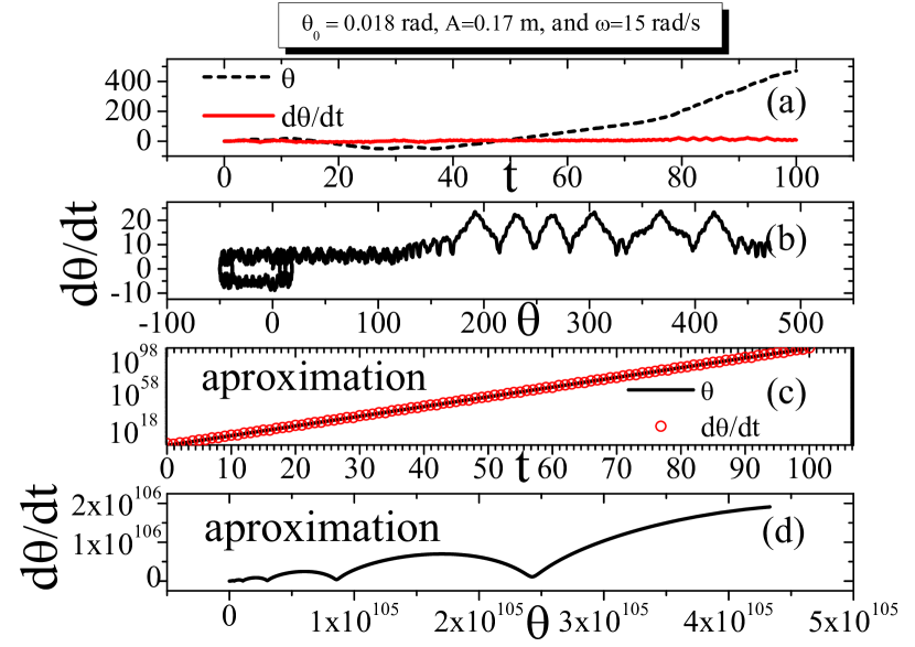
The fact that this figure illustrates a case where the initial condition leads to a non-stable outcome is not os relevant here, since they do not satisfy eq. 10. However what call ones attention is the fact that small initial angle leads to a different different divergence for $\theta(t)$ for large times (instability) whether the one replaces $\sin\theta$ by $\theta$ or not. The plot (2 c) is in mono-log scale since there is a exponential divergence (straight line in this scale) which is more pronounced than in (2 a). Such aspect although seems very simple is simply discarded by some authors in literature. The very different phase diagrams (b) and (d) obtained for these different regimes shows even more our thesis about this topic.

In the results shown in Fig. 2, we consider a larger amplitude $A=0.50$ m. Now, that Eq. 10 is satisfied, we can see a periodic behavior for $\theta$ and $\overset{\cdot}{\theta}$ as function of time in Fig. (3 a) and now beautiful Lissajous plot in the phase space shown in Fig. (3 b).

Figure 3: Results for time evolving and phase diagram considering $\theta_{0}=0.018$ rad, $\omega=15$ rad/s and $A=0.50$ m. (a) Time evolving $\theta$ and $\overset{\cdot}{\theta}$. (b) Corresponding phase diagram $\overset{\cdot}{\theta}\times\ \theta$.

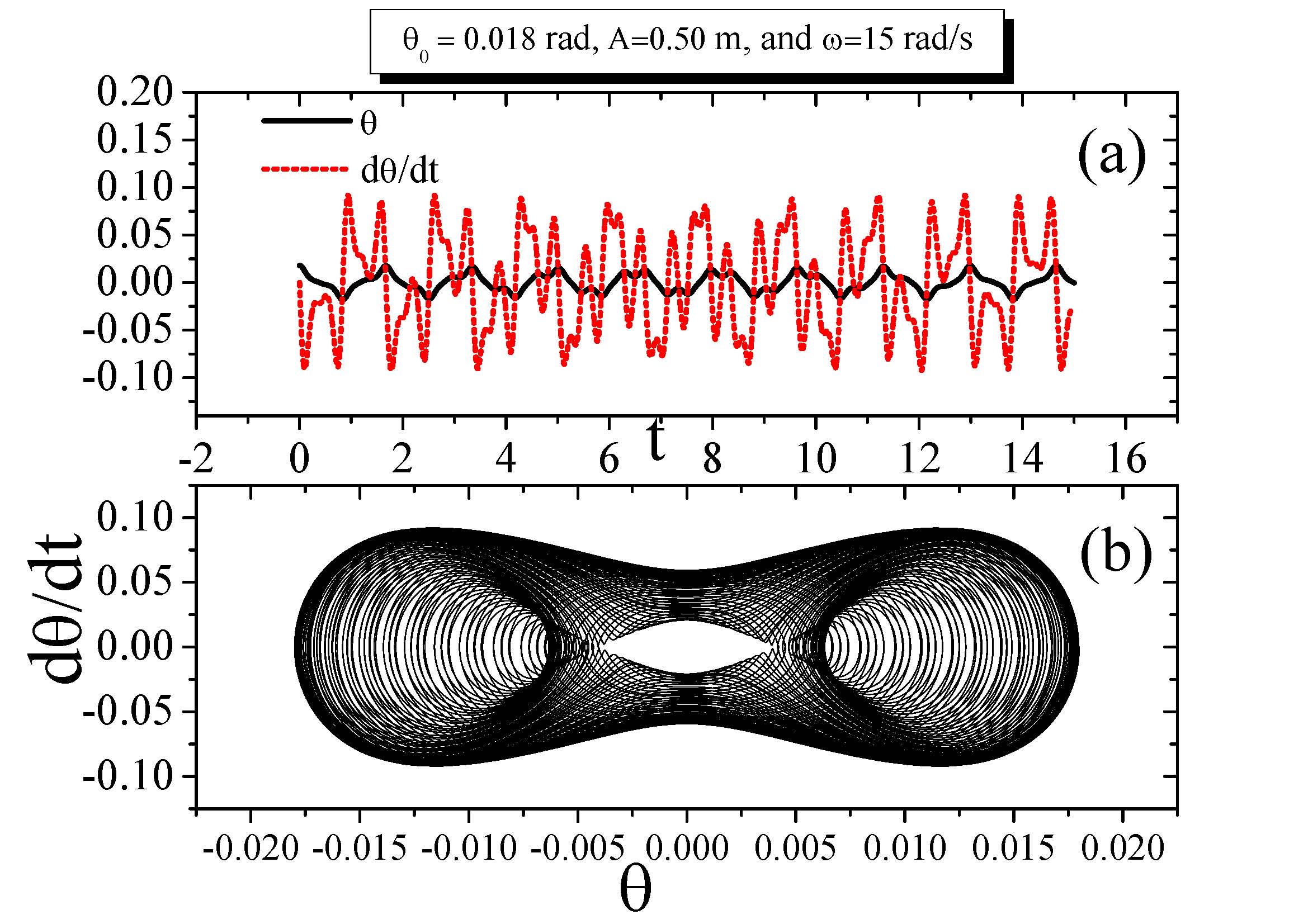
Differently from the Fig. 2 the plots (3c) and (3d) corresponding to small oscillations regime are here omitted since there is no significant difference in the simulations.

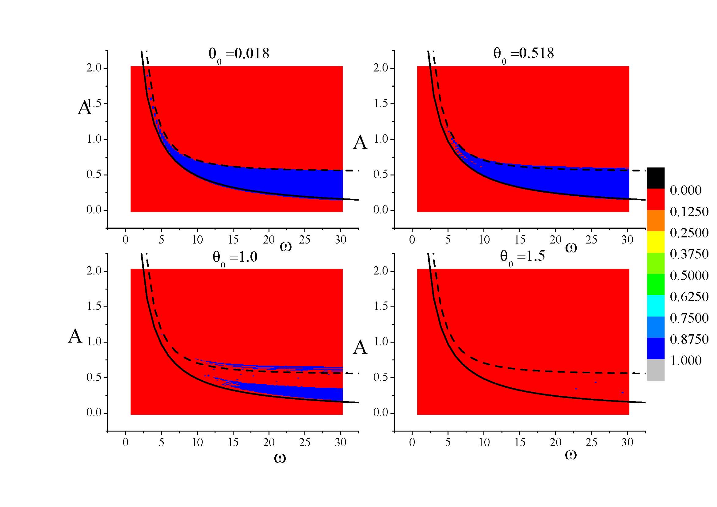
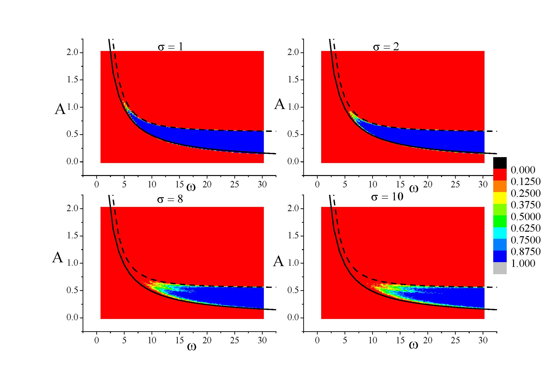
In order to study initial angles’ effects, we analyze the phase diagram $\omega\times A$ obtained via numerical simulations. The diagrams are shown in Fig. 4, and which they correspond to results from Procedure 1: Table 2 (in this case we make $N_{run}=1$). It is important to consider that Eq. 10 determines a lower bound for amplitude: $A_{\min}=\frac{\sqrt{2gl}}{\omega}$. On the other hand, when the amplitude $A$ is increased beyond a certain critical value $A_{\max}$, the pendulum loses its stability again [12, 13, 9] and its evolution cannot be described by effective potential method (perturbative analysis). It is shown in Butikov [9], based in simulation (heuristic) arguments, shows that the solution over the upper boundary of stability has a simple spectral decomposition in only two frequencies: $\omega/2$ and $3\omega/2$, such that $\theta(t)=A_{1}\cos(\omega t/2)+A_{3}\cos(3\omega t/2)$. By using this hypotesis and substituting this solution in Eq. 14 (instead of the exact equation Eq. 1) we have:

$$A<A_{\max}=\frac{l}{4}\left[\sqrt{117+232(\omega_{0}/\omega)^{2}+80(\omega_{0}/\omega)^{4}}-9-4(\omega_{0}/\omega)^{2}\right]$$ (15)

The solid and dashed black curves show respectively the lower (Eq. 10) and upper (Eq. 15) stability domain boundaries. First, we see that the blue region is being destroyed as the initial angle increases, but we need to pay attention to the way it happens. We can observe an interesting effect: there is a set of conditions in the primary stability region that loses its stability so that the region becomes fragmented, while another set above the upper limit becomes stable. The upper limit, established in [9], is really restricted to small angles showing that is based in the approximated equation, which again indicates the importance of the numerical work here. However the lower bound obtained by the effective potential is absolutely respected (not invaded by stability region).

Figure 4: Initial angle effects on the diagram phases $\omega\times A$. The upper (solid) and lower (dashed) curves correspond respectively to the limits established by Eqs. 10 and 15.

In Fig. 5 we show the effects of an additive random noise. We are interested in seeing how the stability diagram is degraded according to the increase of noise variance. Each plot corresponds to a different variance ($\sigma^{2}$). So, we run procedure I (see table 2) with $N_{run}\$= 50 times with different seeds and we calculate the survival probability:

$$p_{survival}=\frac{n_{survival}}{N_{run}}$$

where $n_{survival}$ is the number of times in which our pendulum stabilizes. The color scale are graduated according to the $p_{survival}$-values that were obtained.

Figure 5: External (additive) stochastic noise effects on the diagram phases $\omega\times A$. The different plots correspond to different standard deviations ($\sigma$) of noise $\phi(t)$.

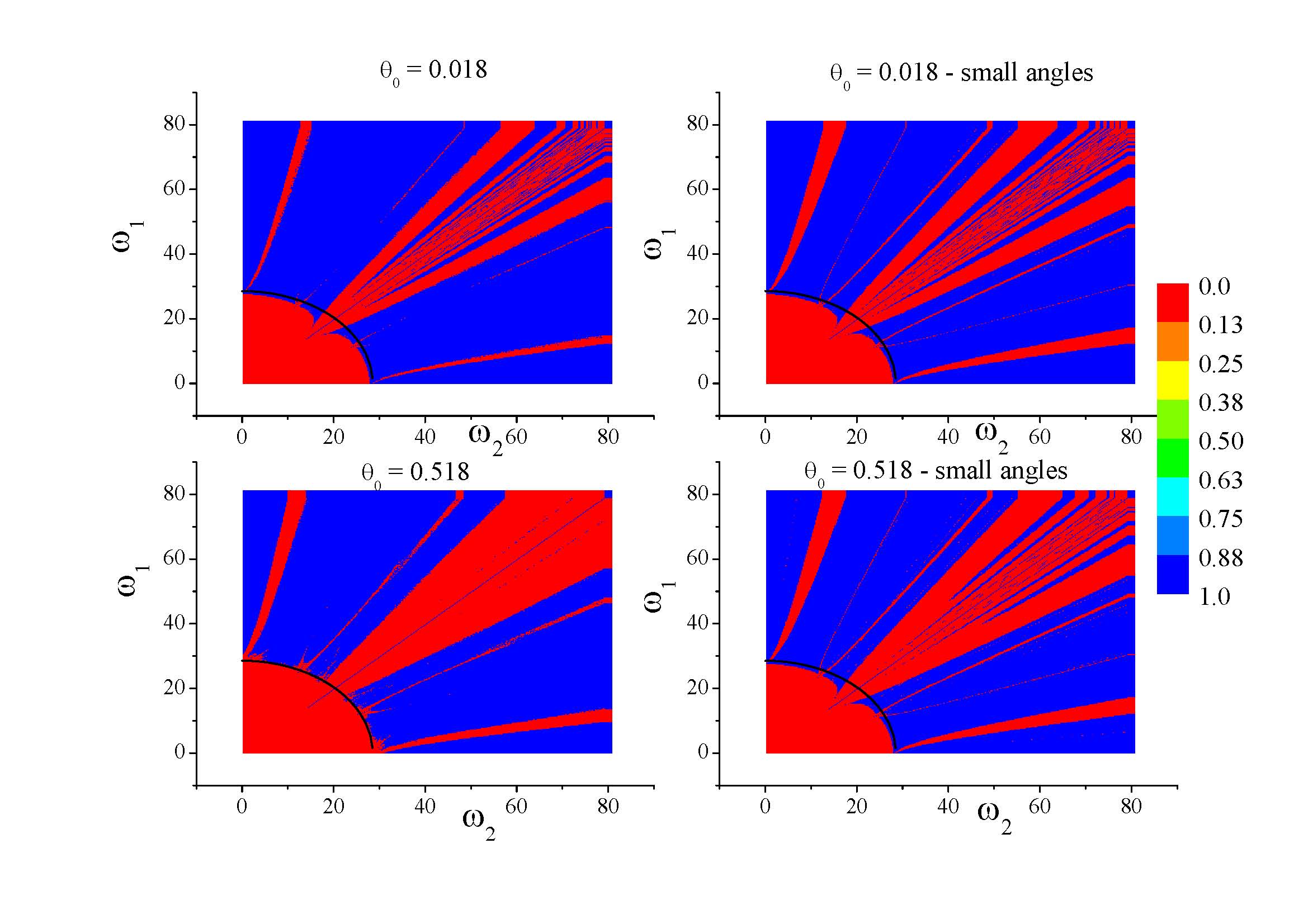
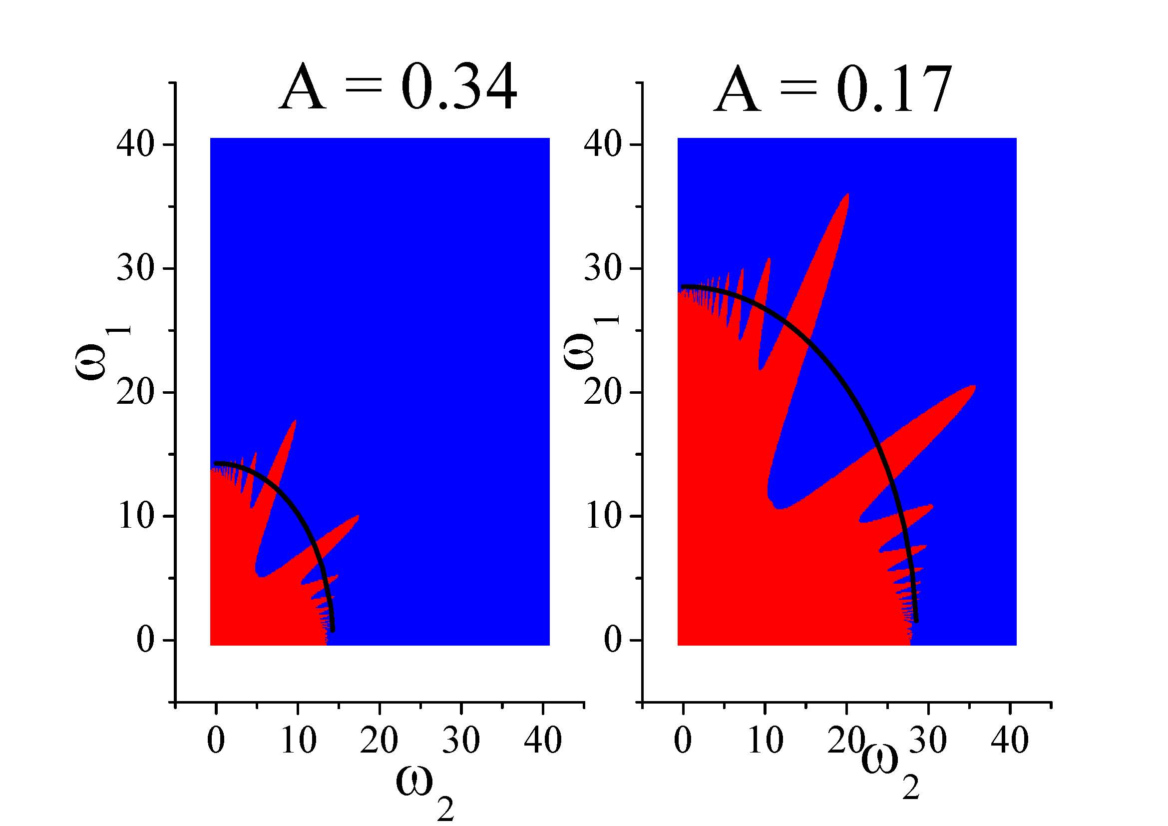
Now we focus our analysis in the case $N=2$, where we make $A_{1}=A_{2}=A$ according to Procedure II: Table 3. The results show a rich structure as we can see in Fig 6. We illustrate two different initial angles for $A=0.17$ recalling that red stands for unstable regions, while blue denotes stabilization. Comparing the figures on the left with the ones on the right (small angles approximation) we can see that it is important to consider $\sin\theta$ and not to make the approximation $\sin\theta\approx\theta$, even for very small angles $\theta_{0}=0.018$ rad $\approx 1^{o}$. We can observe a less restrictive condition $\omega_{1}^{2}+\omega_{2}^{2}\leq\frac{2gl}{A^{2}}$ (a quarter circle, plotted in all figures), which corresponds a condition that $\omega_{1}\approx\omega_{2}=\omega$. Exactly in diagonal the condition goes to $\omega^{2}\leq\frac{gl}{A^{2}}$, which asserts the diagonal line penetrating the 1/4-circle. But, we have more stability regions inside this semi-circle which depend on the proximity of the diagonal. However for $\theta_{0}=0.518$ the system recover the restriction and all quarter of circle is completed but not for the small angles approximation.

However, even more interesting, one should note that it is not always the case that $\omega_{1}$ and $\omega_{2}$, both large, will lead to stabilization. We see branches of unstable regions that remind us of Arnold tongues [16] breaking the stability sea, specially around diagonal the diagonal. It is not our task in this paper to describe the properties of these unstable branches, but they are certainly very rich sets of fractal dimensions [17].

This fractal structure set is deeply modified when $\theta_{0}=0.518$ but only when the numerical solution is not performed in small angle approximations.

Figure 6: Initiall angle effects $N=2$. We used $A=0.17.$

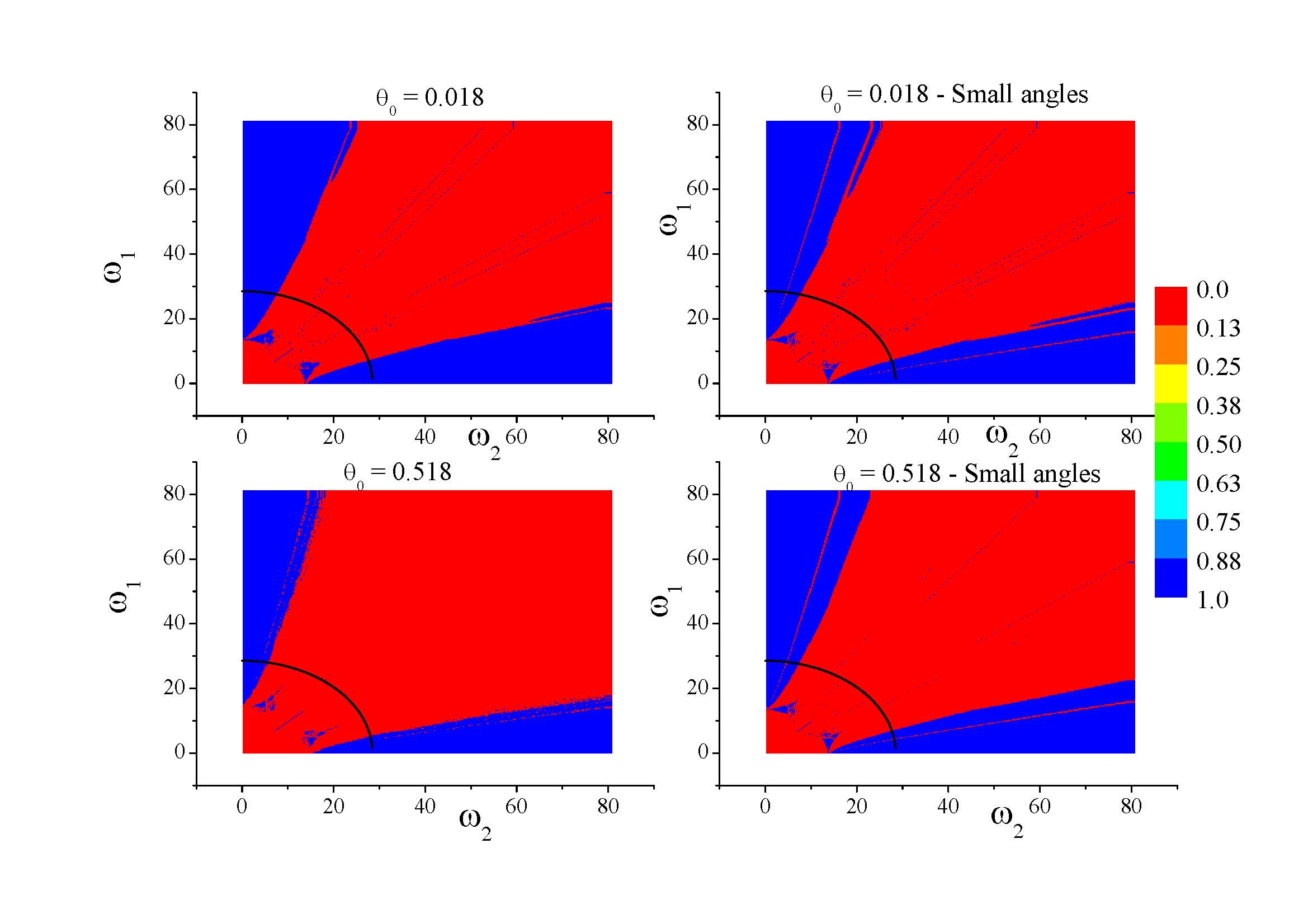
In the Fig. 7 we show the same simulation of Fig. 6 for a larger amplitude $A=0.34$. Now we have a larger instability region. Details of the complexity of unstable branches look less pronounced on the scale of this figure, but it does not mean that they are not there.

Figure 7: Initiall angle effects $N=2$. We used $A=0.34$. Similar to Fig. 6.

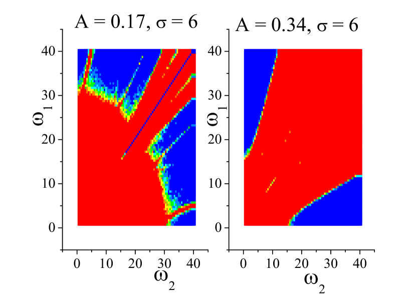
In Fig. 8 we also analyze the effect of noise on the stabilization diagram similar to the case shown in Fig. 5 for $N=1$. Again, $N_{run}=50$ and we observe only one case one case ($\sigma=6$), since the behavior is similar to the case $N=1$, that is, the degraded region enlarges as $\sigma$ enlarges. The case $A=0.34\$m is less sensitive to degradation than $A=0.17$ m.

Figure 8: External Noise effects for effects $N=2$. Comparison for $A=0.17$ and $A=0.34$ for $\sigma=6$. We consider $\theta_{0}=0.018$.

At this point it is important to analyse the results from the perspective of the effective potential method according to Eq. 11.  Recall that we are dealing with the case of $N=2$ and equal amplitudes so that Eq. 11 depends on a variable $T$, which must be function of $\omega_{1}$ and $\omega_{2}$ not always easily determined. So, first we consider what we think that are reasonable choices of $T$ as shown in Fig. 9.

Figure 9: Potential effective for $N=2$ according to Eq. 11. We show some choices for $T$. The best one (that better fits with simulations is to consider the maximal between periods.

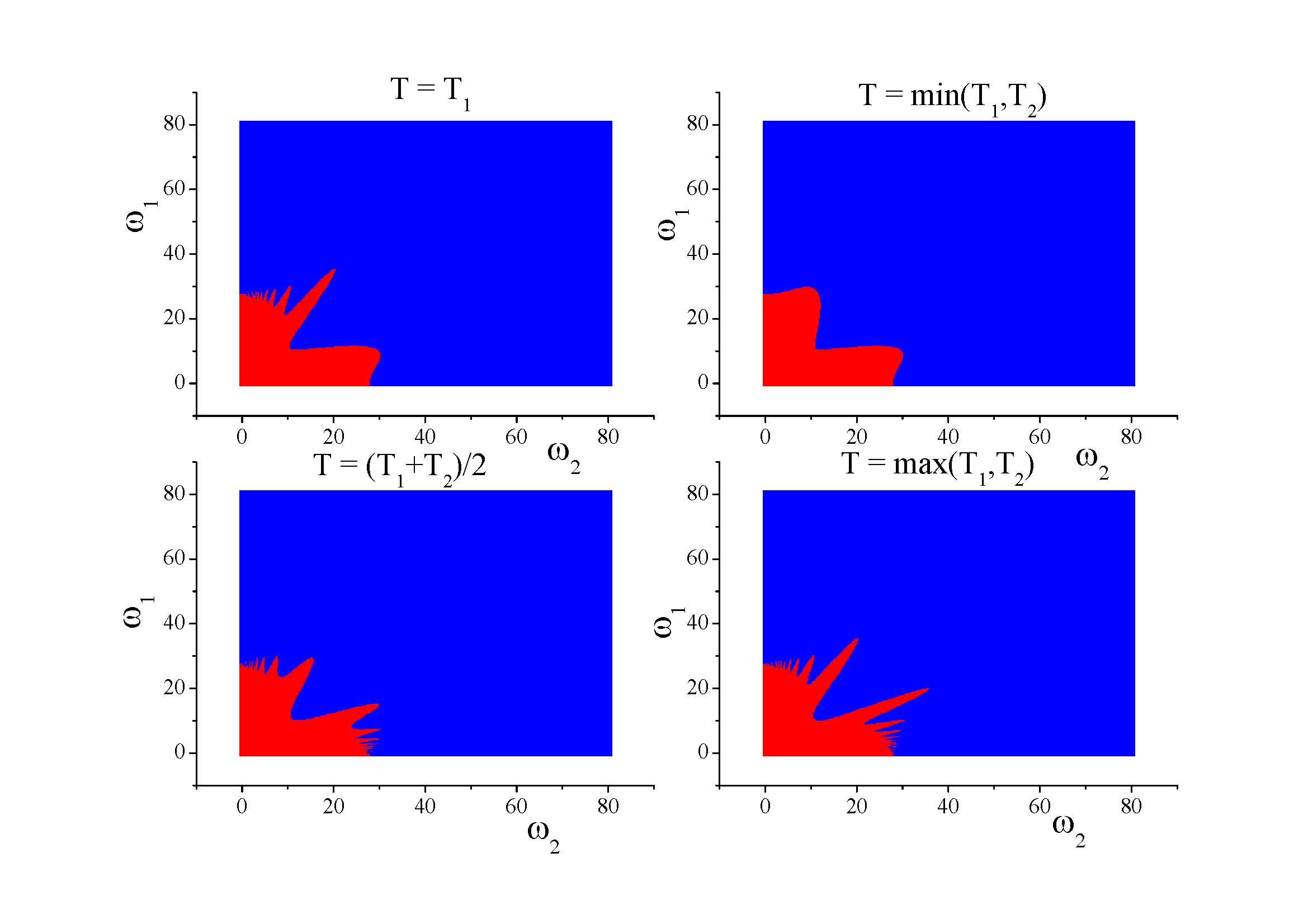
It is clear from these results that the stability diagrams obtained from the effective potential approximation depends strongly on the choice of $T$. From all the numerical simulations, the best option is the choice $T=\max(T_{1},T_{2})$. Another limitation of Eq. 11 is shown in Fig. 10. Here, for different amplitudes we have the same stabilization pattern, except by the fact that the pattern is rescaled with $A$. On the contrary, however, simulations show that $A=0.17$ and $A=0.34$ (please see again Figs. 6 and 7 have completely different diagrams than ones which are shown in the Fig. 10. Just as in the case $N=1$, we must also have an upper limit for the amplitude $A$, however a formulas like Eq. 15 is beyond of our expectations.

Figure 10: Potential effective for $N=2$ according to Eq. 11. We show that for different amplitudes we have the same behavior which shows that effective potential as case $N=1$ has a limitation since numerically we have very different diagrams considering $A=0.17$ and $A=0.34.$

Now let us studying the stochastic stabilization considering $N>2$. Dettman, keating and Prado [8] studied this problem in the context of stochastic stabilization of chaos. And they showed not using our pendulum inverted equation: $\frac{d^{2}\theta}{dt^{2}}=\frac{g}{l}\left(1-\frac{A}{g}\sum\omega_{i}^{2}\cos(\omega_{i}t)\right)\sin\theta$ but so $\frac{d^{2}\theta}{dt^{2}}=\left(1-A\sum_{i=1}^{N}\sin(\omega_{i}t+\varphi_{i})\right)\theta$ that $\theta$ pendulum should be stabilized. Indeed for this particular equation this indeed occurs. We tested this equation with parameters used in this paper: $A=38$, by changing sin by cos (to bring even more proximity with our case) and moreover making $\varphi_{1}=\varphi_{2}=...=0$ which they did not used but which bring even more to similarity with our case. So we also perform 100 frequencies chosen at random from [120, 600] and we do stabilize. However this means to make $g=l=1$ in our case which is not real parameters for our problem. By making $g=l=1$ we also numerically stabilize $\theta$ even considering $\omega_{i}^{2}$ term in the sum which does not appear in [8], but the same does not ocurrs with real values in our case ($l=1.2$ m and $g=9.81$ m/s²). The general arbitrary case $\omega_{0}^{2}=g/l$ with the presence of term $\omega_{i}^{2}$ deserves an special attention and the problem is being studied by the authors in another contribution (see [14])

This negative case leads to look the problem in a alternative point of view as we presented in section 2.

For that we consider the case for $N$ large considering a normalization for amplitude: $A(t)=Ct$, with $CN=a\omega_{\max}$ onde $\omega_{1}$, $\omega_{2}$,…, $\omega_{N}$ are randomly chosen in interval [$0$,$\omega_{\max}$]. Such choice as previously reported must captures the case $N=1$ at least for survival time. So we perform simulations (Procedure III - Table 4) that performs a random formula with $N$ cosines. So we build diagrams $a$ versus $\omega_{\max}$ for survival time (time that pendulum remains stable according the established condition) which can be observed in Fig. 11.

Figure 11: Diagram $a\times\omega_{\max}$. For each pair the point corresponds to survival time (necessary time for the pendulum loses its stability). We can observe a better agreement with region determined by bounds as $N$ enlarges which shows that case $N=1$ has a capture according to amplitude normalization.

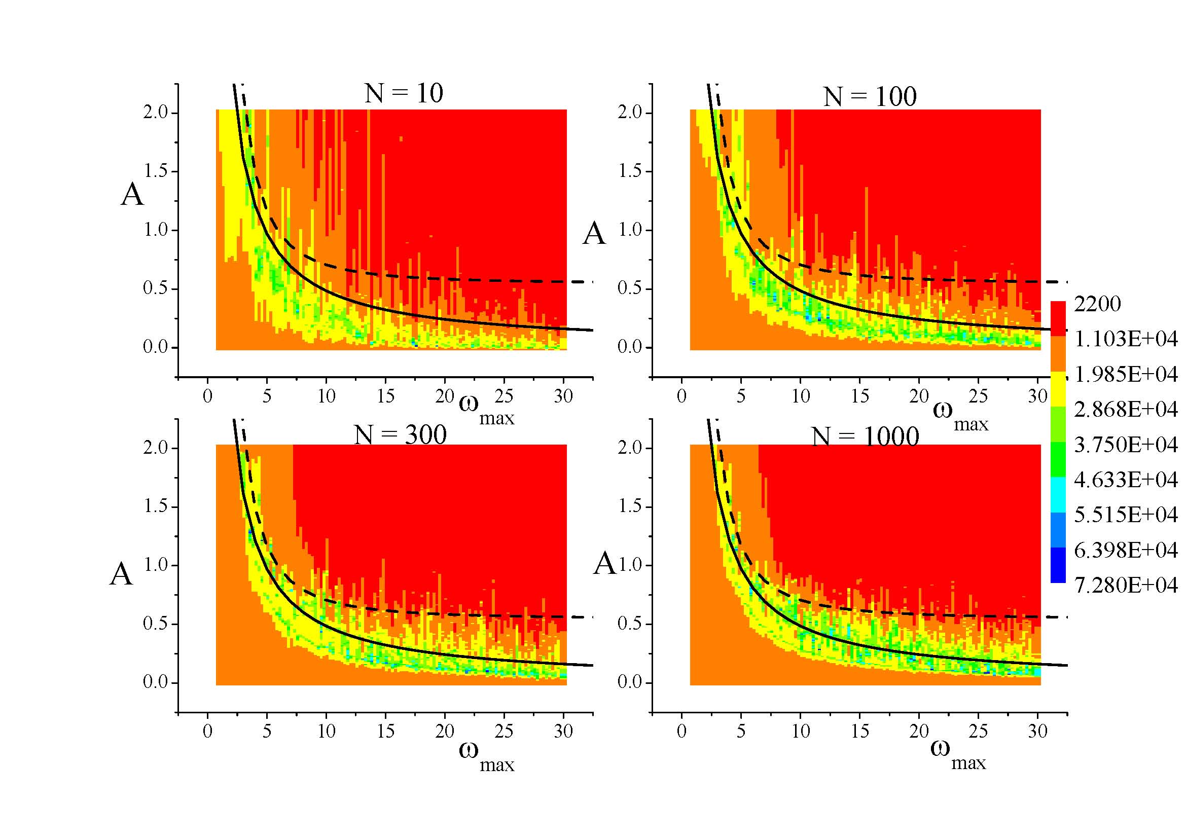
After this interesting phenomena that brings $N$ large for $N=1$, we concentrate our ideas for an interesting optimization process related to stability of pendulum. What the best $N$ for a stabilization of inverted pendulum. This question when performed so free seems to be no interesting. However, the question is, if we would consider an ensemble of formulas by randomly chosen $\omega_{1},...,\omega_{N}$ and $A_{1},...,A_{N}$ in the intervals [$\omega_{\min}=0,\omega_{\max}]$ and $[A_{\min}=0,A_{\max}]$ by repeating $N_{run}=2000$ different formulas and for each choise we observe the stability or not of the pendulum by calculating with this sample a survival probability. We used our Procedure 4: table 5 to calculate such probability. The Fig. 12 shows the survival probability in different situations.

Figure 12: Survival probability according to Procedure IV.

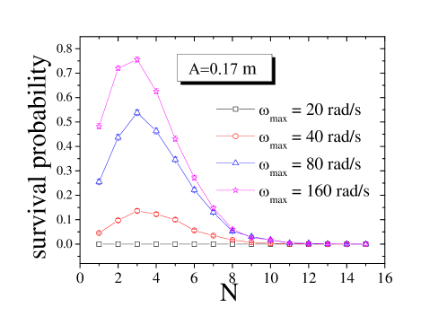
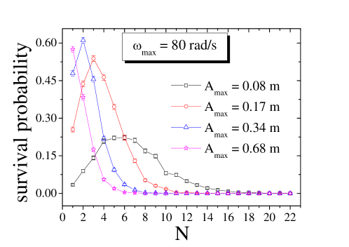
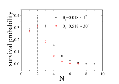
The upper plot in this figure by keeping $A_{\max}=0.17$m and we plot the probability for different values of $\omega_{\max}$. The different frequencies does not change the $N_{\max}$(value that maximizes the survival probability). However the midle figure, shows that keeping $\omega_{\max}$ fixed and by plotting the survival probabilities for different values $A_{\max}$. In this case we change the $N_{\max}$. But it is important to notice that different initial angles does not change $N_{\max}$ as reported in the lower plot in same Fig. 12.

5 Conclusions

In this paper we have detailed the study of inverted pendulum under a parametric excitation in its basis which is described by a superposition of $N$ cosines. In case $N=1$ we explore diagrams $A$ $\times\ \omega$. We show that depending of initial conditions the effective potential method diverges from the numerical simulations, which also occurs in $N=2$ that presents a interesting diagram where stability regions are alternated with no stability ones in a fractal structure. The diagonal $\omega_{1}=\omega_{2}=\omega$ has a important hole in the stability due to the known bating problem in waves. Although the effective potential method is extended for arbitrary $N$ is extended for arbitrary cases its usuality depends on choice of a common period existence and its utility has several limitations by showing the necessity of Runge Kutta integrations of equations which in this paper is separated in four procedures used in each part of our manuscript and showed in details.

For $N>2$ we perform two kind of analysis: a) a discussion about stochastic stabilization and b) optimization of survival probability of pendulum. In this first part (a), starting from hypothesis that inverted pendulum with real parameters cannot be stabilized for $N$ large (this not occurs with suitable choice of parameters) we show that problem for $N$ large can be reduced for $N=1$ if we look for survival time, i.e., the properties of survival time diagram when via a suitable scale in the amplitude are preserved when compared with regular, $N=1$ diagram. In second part (b) we choose randomly choose amplitudes and frequencies in ranges and we calculate the survival probability of pendulum in order to observe the optimal $N$ that maximizes such probability. We have two important three important conclusions here by observing our numerical studies : a) By fixing the upper limit of the frequencies chosen and changing the amplitude, $N_{opt}$ depends on amplitude b) By fixing the upper limit of the amplitude and changing frequency, $N_{opt}$ remains the same. The initial angles seems to be does not change $N_{opt}$.

Acknowledgments – This research was partially supported by the Conselho Nacional de Desenvolvimento Cientifico e Tecnologico (CNPq), under the grant 11862/2012-8. The authors would like to thank Prof. L.G. Brunet (IF-UFRGS) for kindly providing the computational resources from Clustered Computing (ada.if.ufrgs.br) for this work.(2014)

References

- [1] R. A. Ibrahim, J. Vib. Control 12(10), 1093-1170 (2006)
- [2] R. A. Ibrahim, Stabilization and Stochastic Bifurcation with applications in ocean structures, chapter 1, page 1-52 in the Collection: Stochastically Excited Nonlinear Ocean Structures edited by M. F. Shlesinger, T. Swean (1998)
- [3] Y. Kim, S. H. Kim, Y. K. Kwak, Journal of Intelligent and Robotic Systems, 44(1), 25-46 (2005)
- [4] A. Stephenson, The London, Edinburgh and Dublin Philosophical Magazine and Journal of Science 6(15), 233-237 (1908)
- [5] P. L. Kapitza, Zhur. Eksp. i Teoret. Fiz., 21, 588 (1951)
- [6] J. L. Bogdanoff, S. J. Citron, J. Acoust. Soc. Amer. 38, 447-452 (1965)
- [7] R. Yang, Y. Peng, Y. Song, Nonlinear Dyn. 73, 737–749 (2013)
- [8] C. P. Dettmann, J. P. Keating, S. D. Prado, Int. J. Mod. Phys. D. 13(7) 1-8 (2004)
- [9] E. I. Butikov, Am. J. Phys. 69(6) 1-14(2001)
- [10] W. H. Press, S. A. Teukolsky, W. T. Vetterling, B. P. Flannery, Numerical recipes in Fortran 77: the art of scientific computing, Cambridge University Press, 1992
- [11] L. D. Landau, E.M. Lifshitz, Mechanics ( Volume 1 of A Course of Theoretical Physics ) Pergamon Press,1969
- [12] J. A. Blackburn, H. J. T. Smith, N. Groenbech-Jensen, Am. J. Phys. 60(10) 903-908 (1992)
- [13] H. J. T. Smith, J. A. Blackburn, Am. J. Phys. 60(10) 909-911 (1992)
- [14] R. da Silva, S. D. Prado, preprint (2016)
- [15] N. W. McLachlan, Theory and Application of Mathiey Functions, Clarendon Press, Oxford (1947)
- [16] V. I. Arnold, Mathematical Methods of Classical Mechanics, Springer New York (1978)
- [17] E. Ott, Chaos in Dynamical Systems, Cambridge University Press (1993)