Serendipitous discovery of the faint solar twin Inti 1

Abstract

Context. Solar twins are increasingly the subject of many studies owing to their wide range of applications from testing stellar evolution models to the calibration of fundamental observables; these stars are also of interest because high precision abundances could be achieved that are key to investigating the chemical anomalies imprinted by planet formation. Furthermore, the advent of photometric surveys with large telescopes motivates the identification of faint solar twins in order to set the zero point of fundamental calibrations.

Aims. We intend to perform a detailed line-by-line differential analysis to verify whether 2MASS J23263267-0239363 (designated here as Inti 1) is indeed a solar twin.

Methods. We determine the atmospheric parameters and differential abundances using high-resolution ($R\approx 50000$), high signal-to-noise (S/N $\approx$ 110 - 240 per pixel) Keck HIRES spectra for our solar twin candidate, the previously known solar twin HD 45184, and the Sun (using reflected light from the asteroid Vesta).

Results. For the bright solar twin HD 45184, we found $T_{\rm{eff}}=5864\pm 9$ K, log $g=4.45\pm 0.03$ dex, $v_{t}=1.11\pm 0.02$ $\rm{km\ {s}}^{-1}$, and [Fe/H]$=0.04\pm 0.01$ dex, which are in good agreement with previous works. Our abundances are in excellent agreement with the recent high-precision work by Nissen (2015) with an element-to-element scatter of only 0.01 dex. The star Inti 1 has atmospheric parameters $T_{\rm{eff}}=5837\pm 11$ K, log $g=4.42\pm 0.03$ dex, $v_{t}=1.04\pm 0.02$ $\rm{km\ {s}}^{-1}$, and [Fe/H]$=0.07\pm 0.01$ dex that are higher than solar. The age and mass of the solar twin HD 45184 (3 Gyr and 1.05 $\rm{M_{\odot}}$) and the faint solar twin Inti 1 (4 Gyr and 1.04 $\rm{M_{\odot}}$) were estimated using isochrones. The differential analysis shows that HD 45184 presents an abundance pattern that is similar to typical nearby solar twins; this means this star has an enhanced refractory relative to volatile elements, while Inti 1 has an abundance pattern closer to solar, albeit somewhat enhanced in refractories. The abundance pattern of HD 45184 and Inti 1 could be reproduced by adding $\approx 3.5\ \rm{M_{\oplus}}$ and $\approx 1.5\ \rm{M_{\oplus}}$ of Earth-like material to the convective zone of the Sun.

Conclusions. The star Inti 1 is a faint solar twin, therefore, it could be used to calibrate the zero points of different photometric systems. The distant solar twin Inti 1 has an abundance pattern similar to the Sun with only a minor enhancement in the refractory elements. It would be important to analyze other distant solar twins to verify whether they share the Sun’s abundance pattern or if they are enhanced in refractories, as is the case in the majority of nearby solar twins.

1 Introduction

Cayrel de Strobel (1996) defines a solar twin as a star with the same atmospheric parameters (effective temperature, surface gravity, and microturbulent velocity) as the Sun. The first discovery of a solar twin was made by Porto de Mello & da Silva (1997), showing that 18 Sco has atmospheric parameters similar to the Sun. About a decade later three new solar twins were found (King et al. 2005; Meléndez et al. 2006; Takeda et al. 2007), however, these three solar twins and 18 Sco have an overabundance of lithium by a factor of 3-6 higher than the Sun. Later Meléndez & Ramírez (2007) discovered HIP 56948, which is the best solar twin that we have until this point, with stellar parameters and abundances that are similar to the Sun and a low lithium abundance (Meléndez et al. 2012).

In the last few years, the number of solar twins have increased to about 100 (Pasquini et al. 2008; Meléndez et al. 2009; Ramírez et al. 2009; Takeda & Tajitsu 2009; Baumann et al. 2010; Önehag et al. 2011; Datson et al. 2012; do Nascimento et al. 2013; Meléndez et al. 2014b; Porto de Mello et al. 2014; Ramírez et al. 2014). Solar twins could be a useful source for astronomical tests and applications. For example, they could set the zero point of fundamental calibrations (Holmberg et al. 2006; Casagrande et al. 2010; Datson et al. 2014), and they are used to subtract the Sun’s reflected light on asteroids to study their mineralogy (e.g., Lazzaro et al. 2004; Jasmim et al. 2013). Solar twins are also useful for testing stellar interior and evolution models (e.g., Tucci Maia et al. 2015), investigating the chemical evolution of the Galactic disk (Nissen 2015; Spina et al. 2016), studying the rotational evolution of the Sun (do Nascimento et al. 2013, 2014), and measuring distances using spectroscopically identified solar twins (Jofré et al. 2015).

Another application of solar twins is the study of refractories locked by planet formation. Meléndez et al. (2009) found that the difference between abundances of the Sun relative to the solar twins is not zero, showing that the Sun presents abundance anomalies that are correlated with the condensation temperature, $T_{C}$, (Lodders 2003). The Sun presents a deficiency in refractory ($T_{C}\leq 900$ K) relative to volatile ($T_{C}\geq 900$ K) elements, which could be a signature of rocky planet formation (Chambers 2010). Later, Ramírez et al. (2009) supported this idea by studying the abundance of 64 stars with fundamental parameters similar to the Sun; their result showed a strong relation between the abundances and condensation temperature in the majority of their sample. Other authors have been investigating this relation with the existence of planets, although the results are still not conclusive (Gonzalez et al. 2010; Schuler et al. 2011; Adibekyan et al. 2014; Maldonado et al. 2015a; Nissen 2015). Are the abundance anomalies a phenomenon restricted to the solar neighborhood or is it also present in other regions of the Galaxy? This could be investigated using distant solar twins.

In this paper, we report the discovery of the faint solar twin 2MASS J23263267-0239363, which we call Inti 1 for practical reasons.

2 Spectroscopy observations and data reduction

Inti 1 was observed with the HIRES spectrograph (Vogt et al. 1994) at the Keck I telescope at the coordinates ($\alpha$ = 23:26:32.61, $\delta$ = -2:39:35.3) because it was mistaken for the carbon star BPS CS 22949-0037, whose coordinates are actually ($\alpha$ = 23:26:29.80, $\delta$ = -2:39:57.94). This mistake was due to their proximity (Fig. 1). We intended to take two exposures of 1200 s, but after the first exposure it was realized that the star observed was not BPS CS 22949-0037, and the planned exposure sequence was terminated after only one exposure. Fortunately, in the same night we observed the Sun using the same setup. A recent inspection of the spectrum of the wrongly observed target revealed a similarity to the solar spectrum (see Fig. 2), thus making Inti 1 a good candidate to be a solar twin, which we confirmed after high precision analysis. During the same observing run, we also obtained a spectrum for the bright solar twin HD 45184 (e.g., Nissen 2015).

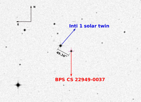
Figure 1: Separation between Inti 1 and BPS CS 22949-0037 is 49.16”. Image from the Aladin Sky Atlas (http://aladin.ustrasbg.fr).

The spectra of HD 45184, Inti 1 and the Sun (using solar reflected light from the Vesta asteroid), were obtained with HIRES/Keck on November 1-3, 2004, covering the wavelength region from 3190-5980 $\AA$. The exposure time for HD 45184, Inti 1 and Vesta were 2$\times$300 s, 1200 s, and 100 s. The spectral resolution, $R=\lambda/\lambda\Delta$ is about 50000, while the signal-to-noise ratios (S/N) estimated for HD 45184, Inti 1 and Vesta are 160, 110 and 240 per pixel.

The spectra were extracted using the MAKEE pipeline that was specifically designed by T. Barlow to reduce HIRES spectra. The standard procedure is followed with bias subtraction, flat fielding, sky subtraction, order extraction, and wavelength calibration. We note that MAKEE already applies the heliocentric correction, so that the output wavelengths are heliocentric. Further processing was performed with IRAF.

We estimated the radial velocity of the star using the rvidlines task in IRAF, and then the spectrum was corrected to the rest frame with the dopcor task. The spectra were normalized using IRAF’s continuum task with orders of the polynomial spline varying from 1 to 5 for each order. In Fig. 2 we show a part of the reduced spectra of HD 45184, Inti 1, and the Sun in the region 5321-5336 $\AA$, where we can see that both stars have an impressive resemblance to the Sun.

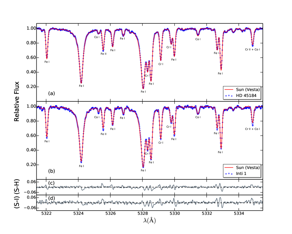
Figure 2: Comparison between the spectra of HD 45184, Inti 1, and the Sun in the region 5321-5336 $\AA$. Panel (a) shows the spectra of HD 45184 (blue open circles) and the Sun (red solid line). Panel (b) shows the spectra of the Sun (red solid line) and candidate solar twin Inti 1 (blue open circles), showing a striking similarity. The different chemical composition is revealed through careful line- by-line measurements. Residuals between the Sun and HD 45184 (S-H), and the Sun and Inti 1 (S-I) are shown in the panel (c) and (d), respectively.

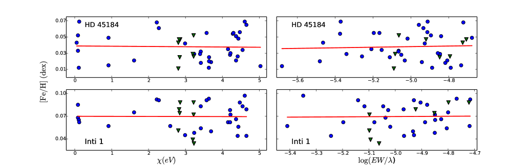
Figure 3: Differential iron abundances as a function of excitation potential (left panels) and reduced equivalent width (right panels) for the solar twin HD 45184 and Inti 1. Blue filled circles and green filled triangles represent Fe I and Fe II, while red lines are the fits.

The similarity between Inti 1 and the Sun also extends to colors; using VIZIER, we found the magnitudes: $\mathrm{V}=12.857\pm 0.028$, $\mathrm{B}=13.516\pm 0.032$, $\mathrm{I}=12.045\pm 0.072$, $\mathrm{J}=11.559\pm 0.023$, $\mathrm{H}=11.247\pm 0.023$, $\mathrm{K}=11.168\pm 0.024$, $\mathrm{W1}=11.125\pm 0.023$, and $\mathrm{W2}=11.180\pm 0.022$. Inti 1 and the Sun present similar color magnitudes (Table 1) reinforcing the idea that it is a solar twin. Extinction coefficients for $\mathrm{(B-V)}$, $\mathrm{(V-I)}$, $\mathrm{(V-J)}$, $\mathrm{(V-H)}$, $\mathrm{(V-K)}$ photometry were taken from Ramírez & Meléndez (2005) and for $\mathrm{(V-W1)}$, $\mathrm{(V-W2)}$ from Yuan et al. (2013). For the extinction correction, we used $\mathrm{E(B-V)}=0.044\pm 0.002$ , that is from the reddening maps of Schlegel et al. (1998), with the correction proposed by Schlafly & Finkbeiner (2011).

Table 1: Comparison of colors of the Sun and Inti 1.

Color	Inti 1		Sun
	Observed	Derredened
$\mathrm{(B-V)}^{a}$	$0.659\pm 0.042$	$0.615\pm 0.042$	$0.653\pm 0.005$
$\mathrm{(V-I)}^{a}$	$0.812\pm 0.077$	$0.755\pm 0.077$	$0.702\pm 0.010$
$\mathrm{(V-J)}^{b}$	$1.298\pm 0.036$	$1.203\pm 0.036$	$1.198\pm 0.005$
$\mathrm{(V-H)}^{b}$	$1.610\pm 0.036$	$1.500\pm 0.036$	$1.484\pm 0.009$
$\mathrm{(V-K)}^{b}$	$1.689\pm 0.036$	$1.570\pm 0.036$	$1.560\pm 0.008$
$\mathrm{(V-W1)}^{b}$	$1.731\pm 0.036$	$1.603\pm 0.036$	$1.608\pm 0.008$
$\mathrm{(V-W2)}^{b}$	$1.676\pm 0.035$	$1.556\pm 0.035$	$1.583\pm 0.008$

3 Abundance analysis

We adopted the line list of Meléndez et al. (2014a) to measure the equivalent widths (EWs) of the spectral lines; we used the IRAF splot task and fitted the line profiles using Gaussians. The pseudo-continuum regions were determined as in Bedell et al. (2014) in a window of 8 $\AA$.

Table 2: Comparison of stellar parameters for the solar twin HD 45184

$T_{\rm{eff}}$	error	log $g$	error	$\rm{[Fe/H]}$	error	$v_{t}$	error	Age	error	Mass	error	Source
(K)	(K)	(dex)	(dex)	(dex)	(dex)	(km $\rm{s}^{-1}$)	(km $\rm{s}^{-1}$)	(Gyr)	(Gyr)	$\rm{M}_{\odot}$	$\rm{M}_{\odot}$
5864	9	4.45	0.03	0.040	0.010	1.11	0.02	3.0	1.2	1.05	0.01	This work
5873	18	4.41	0.04	0.070	0.016	1.03	0.04	3.7	1.2	1.06	0.02	1$\dagger$
5871	6	4.45	0.01	0.047	0.006	1.06	0.02	2.7	0.5	1.06	0.01	2$\dagger$
5833	10	4.37	0.02	0.010	0.010	1.04	0.06	…	…	…	…	3$\dagger$
5849	86	4.45	0.11	0.040	0.090	1.11	0.09	4.4	2.3	1.03	0.05	4$\dagger$
5869	14	4.47	0.02	0.040	0.010	1.03	0.04	2.3	…	1.05	…	5*$\dagger$
5863	5	4.44	0.01	0.040	0.004	1.05	0.02	2.9	0.5	1.06	0.01	6

In order to compute the stellar parameters, we employed the MARCS model atmospheres (Gustafsson et al. 2008) and the 2014 version of the local thermodynamic equilibrium (LTE) code MOOG (Sneden 1973). The LTE is adequate for differential studies of solar twins, as the differential NLTE (non-LTE) effects in solar twins are negligible (Meléndez et al. 2012; Monroe et al. 2013).

Spectroscopic equilibrium is used to determine the effective temperature ($T_{\rm{eff}}$), surface gravity (log $g$), metallicity ([Fe/H]), and microturbulent velocity ($v_{t}$). This is performed by imposing the relative excitation and ionization equilibrium, and evaluating the lack of dependence of differential iron abundance with reduced equivalent width ($\rm{EW}/\lambda$). All the calculations are strictly differential ($\Delta A_{i}$).

As a first step, we determined the abundances of the Sun ($A^{\odot}_{i}$) for each line, adopting the standard solar parameters ($T_{\rm{eff}}=5777$ K, log $g=4.44$ dex (Cox 2000), and $v_{t}=1.00\$km$\ \rm{s}^{-1}$ as in Ramírez et al. (2014)). The second step is the determination of stellar parameters of Inti 1; initially we set as the atmospheric parameters those of the Sun, then the abundances ($A^{\star}_{i}$) were found running the MOOG code. We achieved the spectroscopic solution varying the values for the parameters until achieving differential spectroscopic equilibrium (Fig. 3).

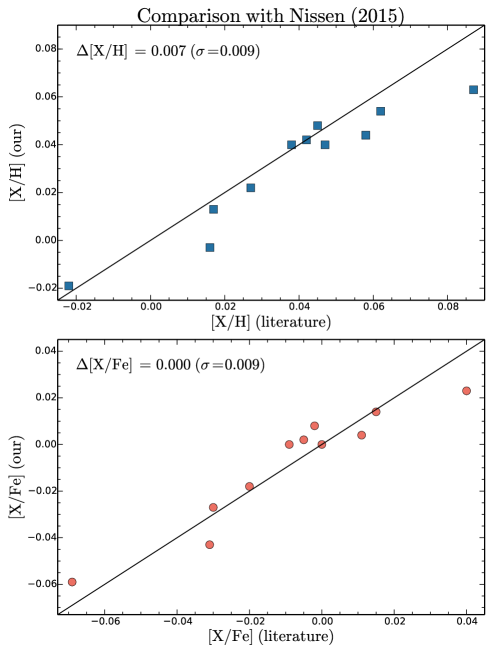
Figure 4: Upper panel: Comparison between our [X/H] ratios and those from the high precision work by Nissen (2015). Lower panel: As above for [X/Fe].

We first study the bright solar twin HD 45184 to validate our method. The stellar parameters that we found are $T_{\rm{eff}}=5864\pm 9$ K, log $g=4.45\pm 0.03$ dex, $v_{t}=1.11\pm 0.02$ $\rm{km\ {s}}^{-1}$, and [Fe/H]$\ =0.04\pm 0.01$ dex. These values are in a good agreement with all previous works found in the literature, as shown in Table 2, as well as in good accord with the weighted mean value, $T_{\rm{eff}}=5863\pm 5$ K, log $g=4.44\pm 0.01$ dex, $v_{t}=1.05\pm 0.02$ $\rm{km\ {s}}^{-1}$, and [Fe/H]$\ =0.040\pm 0.004$ dex. The stellar parameters found for Inti 1 are $T_{\rm{eff}}=5837\pm 11$ K, log $g=4.42\pm 0.03$ dex, $v_{t}=1.04\pm 0.02$ km $\rm{s}^{-1}$, and [Fe/H]$\ =0.07\pm 0.01$ dex. According to the solar twin definition of Ramírez et al. (2009), a solar twin should be within $\Delta T_{\rm{eff}}=100$ K, $\Delta$log$\ g=0.1$ dex, and $\Delta$[Fe/H] = 0.1 dex of the Sun; our results agree with this definition, hence, Inti 1 is a solar twin.

Once the atmospheric parameters were set, we measured the abundances of 18 elements other than iron using atomic lines: C, Na, Mg, Si, Ca, Sc, Ti, Cr, Mn, Co, Ni, Cu, Zn, Y, Zr, Ce, and Nd. For carbon we also used CH molecular lines and for nitrogen we used NH. The hyperfine correction was made for Mn, Co, Y, and Cu, adopting the HFS data from Meléndez et al. (2014a). We compare our abundances for the bright solar twin HD 45184 with the most precise abundances available (Fig. 4), which are from Nissen (2015). We found a difference (this work - Nissen (2015)) of $\Delta$[X/H] = 0.007 ($\sigma$ = 0.009 dex) and $\Delta$[X/Fe] = 0.000 ($\sigma$ = 0.009 dex). This shows that our precision is about 0.01 dex. We also compared with two other works in the literature, resulting in $\Delta$[X/H] = 0.023 ($\sigma$ = 0.016 dex) and $\Delta$[X/Fe] = - 0.007 ($\sigma$ = 0.016 dex) for Spina et al. (2016), and $\Delta$[X/H] = 0.014 ($\sigma$ = 0.030 dex) and $\Delta$[X/Fe] = 0.004 ($\sigma$ = 0.030 dex) for González Hernández et al. (2010).

$\begin{array}[]{c}\includegraphics[width=256.0748pt]{mass-age-hd}\\ \includegraphics[width=256.0748pt]{mass-age-inti}\end{array}$

Figure 5: Age probability distribution of HD 45184 (upper panel) and Inti 1 (lower panel). The dashed lines represent the most probable age. The different regions represent $\pm$ 1 sigma and $\pm$ 2 sigma confidence level.

The differential abundances for HD 45184 and Inti 1 are presented in Table 4, including the observational errors and systematic errors (due to uncertainties in the stellar parameters), and we also included the total error obtained from quadratically adding the statistical and systematic errors.

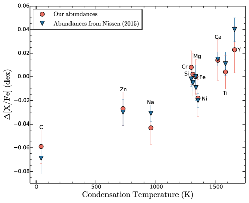
Figure 6: Comparison between our abundance and Nissen (2015), as a function of condensation temperature (Lodders 2003).

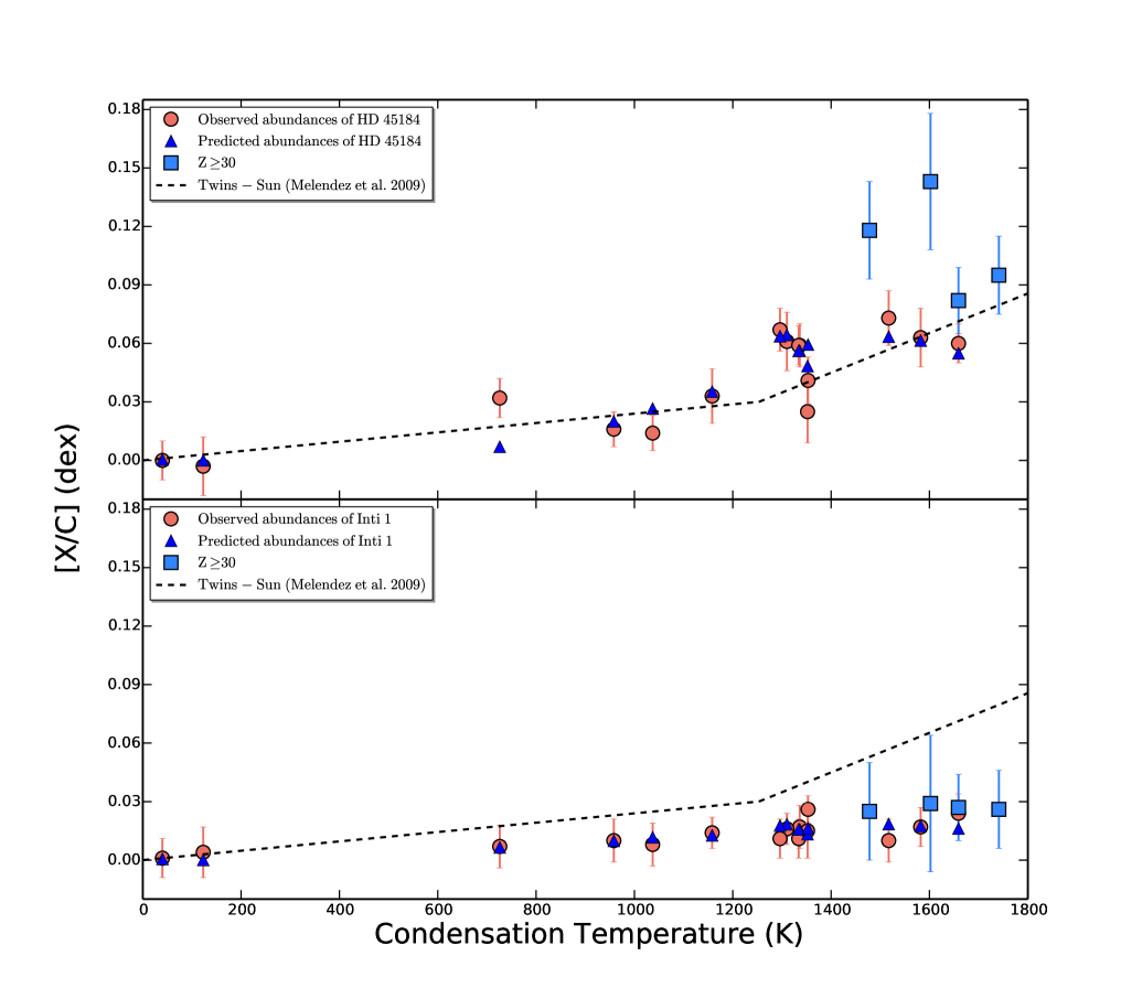
Figure 7: Upper panel: Abundance pattern of HD 45184 (red filled circles) versus condensation temperature. We reproduce the chemical pattern of HD 45184 (blue filled triangles) adding $3.5\ \mathrm{M_{\oplus}}$ of Earth-like material to the convective zone of the Sun. Lower panel: The differential abundance ratios of Inti 1 (red filled circles) relative to the Sun as a function of condensation temperature. The mean abundance pattern of 11 solar twins studied by Meléndez et al. (2009) is represented by the black dashed line. We could reproduce the trend of Inti 1 (blue filled triangles), adding $1.5\ \mathrm{M_{\oplus}}$ of Earth-like material to the convective zone of the Sun. Neutron capture elements are represented by squares in both panels.

We computed the mass and age of HD 45184 and Inti 1 using our atmospheric parameters and employing the $\mathrm{q}^{2}$ (qoyllur-quipu) code . This code is based in python and was developed by Ramírez et al. (2014), to determine the masses and ages of stars using the Yonsei-Yale isochrones (e.g., Yi et al. 2001).

Our results show a mass of 1.05 $\rm{M_{\odot}}$ and 1.04 $\rm{M_{\odot}}$ for HD 45184 and Inti 1. The age obtained is about 3 Gyr and 4 Gyr for HD 45184 and Inti 1 (Fig. 5). The mass and age of HD 45184 are in excellent agreement with the weighted mean value found in the literature (Table 2). The Yonsei-Yale grids of stellar models do not include nonstandard physics such as those included in studies of lithium depletion (Do Nascimento et al. 2009; Denissenkov 2010; Li et al. 2012). We tested our method for the star 18 Sco, which was analyzed using nonstandard models by Li et al. (2012), and found the same mass and age. Furthermore, Meléndez et al. (2014a) shows that the exact choice of isochrone do not have an important impact on the masses and ages relative to the Sun.

4 Abundance trends and results

A comparison between our chemical pattern and that of Nissen (2015) is shown in Fig. 6. It is reassuring that we get the same trend as the precise work by Nissen (2015). In Fig. 7 we show the differential abundances normalized to carbon for HD 45184 (upper panel) and Inti 1 (lower panel), as a function of condensation temperature (Lodders 2003). The chemical pattern of HD 46184 follows the abundance pattern of the fit of the mean trend of 11 solar twins studied by Meléndez et al. (2009), as shown by the dashed lines after a vertical shift. Inti 1 has an abundance pattern closer to solar, albeit slightly enhanced in refractories. The offset between the refractory and volatiles elements of HD 45184 and Inti 1 are 0.076 dex and 0.025 dex, respectively.

Table 3: Fundamental parameters for Inti 1

Inti 1	Parameters
$T_{\rm{eff}}$	$5837\pm 11$ K
log $g$	$4.42\pm 0.03$ dex
$\rm[Fe/H]$	$0.07\pm 0.01$ dex
$v_{t}$	$1.04\pm 0.02$ km $\rm{s}^{-1}$
Mass	$1.04^{+0.01}_{-0.08}$ $\ \mathrm{M_{\odot}}$ **
Distance	$389.70\pm 36.00$ pc *
Convective Mass	$0.019$ $\ \mathrm{M_{\odot}}$ ***
Age	$4.00^{+1.00}_{-1.26}$ Gyr **
logL	$0.06\pm 0.032\ \mathrm{L_{\odot}}$ **
$\mathrm{M_{V}}$	$4.68^{+0.08}_{-0.07}$ mag **
Radius	$1.05\pm 0.04\ \mathrm{R_{\odot}}$ **

Nissen (2015) showed that the [Y/Mg] ratio is an age indicator. Using his relation, we estimate ages of 3.7 $\pm$ 0.6 Gyr and 4.1 $\pm$ 0.6 Gyr for HD 45184 and Inti 1; these results are in agreement with the isochronal ages computed by using $\mathrm{q}^{2}$.

Following Chambers (2010), we computed the mass of rocky material needed to reproduce the abundance trend of HD 45184 and Inti 1. Our results show a value of $3.5\pm 1\ \rm{M_{\oplus}}$ of refractory elements using a mixture of Earth-like and CM-chondrite-like material for HD 45184 and $1.5\pm 1\ \rm{M_{\oplus}}$ for Inti 1. These patterns are represented by blue filled triangles in Fig. (7).

Table 4: Stellar abundances [X/H] and errors for HD 45184 and Inti 1.

				HD 45184
Element	$\Delta$ [X/H]	$\Delta T_{\mathrm{eff}}$	$\Delta$log $g$	$\Delta v_{t}$	$\Delta$[Fe/H]	Param	Obs	Total
	LTE	$\pm$9 K	$\pm$0.03 dex	$\pm$0.02 km s-1	$\pm$0.01 dex
	(dex)	(dex)	(dex)	(dex)	(dex)	(dex)	(dex)	dex
C	-0.019	0.005	0.007	0.000	0.000	0.009	0.006	0.010
Na	-0.003	0.004	0.002	0.000	0.000	0.004	0.008	0.009
Mg	0.040	0.007	0.003	0.004	0.000	0.009	0.007	0.011
Si	0.042	0.002	0.002	0.000	0.001	0.003	0.001	0.015
Ca	0.054	0.005	0.003	0.004	0.000	0.007	0.012	0.014
Sc	0.041	0.007	0.003	0.000	0.000	0.008	0.006	0.010
Ti	0.044	0.009	0.002	0.003	0.000	0.010	0.012	0.015
Cr	0.048	0.007	0.001	0.004	0.000	0.008	0.008	0.011
Mn	0.014	0.006	0.001	0.003	0.000	0.007	0.012	0.014
Fe	0.040	0.007	0.001	0.006	0.000	0.010	0.003	0.010
Co	0.006	0.006	0.003	0.001	0.000	0.007	0.014	0.016
Ni	0.022	0.004	0.001	0.003	0.001	0.005	0.011	0.012
Cu	-0.005	0.004	0.002	0.002	0.001	0.005	0.007	0.009
Zn	0.013	0.002	0.001	0.007	0.002	0.008	0.006	0.010
Y	0.063	0.001	0.010	0.009	0.002	0.014	0.010	0.017
Zr	0.076	0.001	0.013	0.004	0.002	0.015	0.014	0.020
Ce	0.099	0.002	0.014	0.002	0.003	0.015	0.020	0.025
Nd	0.124	0.002	0.014	0.001	0.003	0.014	0.032	0.035
C(CH)	-0.021	0.007	0.001	0.001	0.006	0.009	0.013	0.016
N(NH)	0.003	0.009	0.001	0.000	0.006	0.011	0.011	0.015
				Inti 1
Element	$\Delta$ [X/H]	$\Delta T_{\mathrm{eff}}$	$\Delta$log $g$	$\Delta v_{t}$	$\Delta$[Fe/H]	Param	Obs	Total
	LTE	$\pm$11 K	$\pm$0.03 dex	$\pm$0.02 km s-1	$\pm$0.01 dex
	(dex)	(dex)	(dex)	(dex)	(dex)	(dex)	(dex)	dex
C	0.059	0.006	0.008	0.001	0.000	0.010	0.004	0.011
Na	0.069	0.005	0.001	0.000	0.000	0.005	0.010	0.011
Mg	0.076	0.009	0.005	0.004	0.001	0.011	0.003	0.011
Si	0.075	0.003	0.002	0.001	0.001	0.004	0.007	0.008
Ca	0.069	0.007	0.004	0.000	0.004	0.009	0.007	0.011
Sc	0.083	0.009	0.003	0.001	0.000	0.010	0.007	0.012
Ti	0.076	0.010	0.001	0.003	0.000	0.010	0.006	0.012
Cr	0.066	0.010	0.003	0.006	0.000	0.012	0.006	0.013
Mn	0.073	0.007	0.001	0.003	0.001	0.008	0.001	0.008
Fe	0.070	0.009	0.001	0.005	0.000	0.010	0.003	0.011
Co	0.074	0.009	0.003	0.001	0.001	0.010	0.010	0.014
Ni	0.085	0.006	0.000	0.003	0.001	0.007	0.003	0.007
Cu	0.067	0.006	0.002	0.002	0.001	0.007	0.010	0.012
Zn	0.066	0.002	0.000	0.007	0.003	0.008	0.007	0.011
Y	0.086	0.001	0.011	0.009	0.003	0.015	0.006	0.016
Zr	0.085	0.001	0.014	0.003	0.003	0.016	0.008	0.017
Ce	0.084	0.003	0.015	0.002	0.003	0.016	0.007	0.017
Nd	0.088	0.003	0.015	0.002	0.003	0.016	0.003	0.016
C(CH)	0.062	0.009	0.000	0.001	0.008	0.012	0.010	0.016
N(NH)	0.063	0.010	0.001	0.001	0.008	0.013	0.002	0.013

We developed a code in python to make this calculation easier. The code first computes the convective mass of a solar twin, and then estimates the mass of the rocky material missing in the convective zone. The convective mass is calculated making a double interpolation to the mass and metallicity of the solar twin. The convective masses adopted for this calculation are from Siess et al. (2000) .

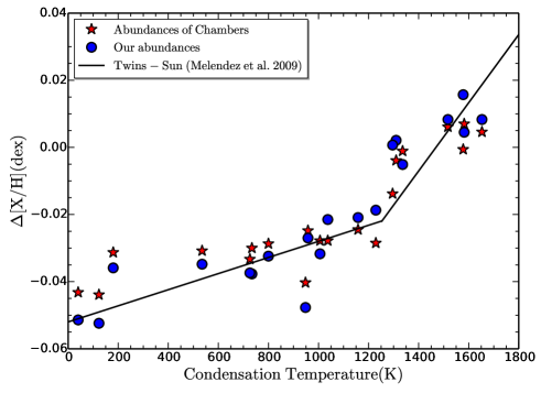
Figure 8: Composition of the solar photosphere adding $4\ \rm{M}_{\oplus}$ in mixture of rocky material (Earth plus meteoritic) to the convective zone of the Sun.

Once the convective mass is obtained, the code computes the convective mass of each element present in the Sun, adopting the abundances of Asplund et al. (2009). Adopting the same approach, we use the abundances of Wasson & Kallemeyn (1988) and Allègre et al. (2001) for the chemical composition of CM chondrites and the Earth. This is explained in more detail in appendix References (see also Chambers (2010); Mack et al. (2014)). All our calculations for Inti 1 are listed in Table 3.

To verify our results, we reproduced the calculation of Chambers (2010) in Fig. 8, adding a mixture of $2\ \rm{M_{\oplus}}$ of Earth-like material and $2\ \rm{M_{\oplus}}$ of chondrite-like material. Our abundances are represented by blue filled circles, while the abundances of Chambers by filled red stars. Our results agree well with the calculation of Chambers, who used the same meteoritic composition as us, but he adopted another reference for the Earth (Waenke & Dreibus 1988).

5 Conclusions

Our atmospheric parameters computed relative to the Sun for HD 45184 are $T_{\rm{eff}}=5864\pm 9$ K, log $g=4.45\pm 0.03$ dex, $v_{t}=1.11\pm 0.02$ $\rm{km\ {s}}^{-1}$, and [Fe/H]$=0.04\pm 0.01$ dex, and for the faint solar twin Inti 1 are $T_{\rm{eff}}=5837\pm 11$ K, log $g=4.42\pm 0.03$ dex, $v_{t}=1.04\pm 0.02$ $\rm{km\ {s}}^{-1}$, and [Fe/H]$=0.07\pm 0.01$ dex, meaning that our star Inti 1 is a solar twin (Ramírez et al. 2009). In Table 1 we showed that the colors of Inti 1 are identical to the Sun within errors. Thus our faint solar solar twin and the distant solar twin found by do Nascimento et al. (2013) could be used to calibrate different photometric surveys.

The abundances of HD 45184 shows an excellent agreement with the highly precise work by Nissen (2015). HD 45184 and Inti 1 present enhancement in the refractory elements compared to volatiles species with an offset of 0.076 dex and 0.025 dex, respectively. This demonstrates that the same chemical anomalies found when the Sun is compared to local solar twins are also present when compared to distant solar twins (albeit the refractory enhancement of Inti 1 is smaller than for the nearby solar twin HD 45184). Using our code and theoretical models from Siess et al. (2000), we estimated the mass of rocky material present in the convective zone for HD 45184 ($\approx 3.5\ \rm{M_{\oplus}}$) and Inti 1 ($\approx 1.5\ \rm{M_{\oplus}}$), relative to the Sun.

The lithium abundances are usually determined from the 6708 Å resonance line (or sometimes from the 6104 Å subordinate line). Hence, they were not measured because of our limited spectral coverage (3190-5980 Å). However, future observations will allow us to determine the Li abundance of Inti 1, and verify if the star follows the lithium-age correlation (e.g., Monroe et al. 2013).

Appendix A Estimating the missing mass of rocky material

Adopting the abundance of Asplund et al. (2009) for the chemical composition of the Sun ($\rm{A_{sun}}$), and using [Fe/H] of a given star, we could estimate the mass of rocky material missing from its convective zone. First we have to compute the mass of each element, which is given by

$$\rm{X_{conv\_mass}}=A\times 10^{(\mathrm{\rm{A_{sun}}\ +\ [Fe/H]})},$$ (1)

where A is the atomic weight. Then the convective mass of each element is given by

$$Convective_{mass}=\rm{M_{conv}\times M_{\odot}}\times\frac{X_{conv\_mass}}{\sum X_{conv\_mass}},$$ (2)

where $\rm{M_{conv}}$ is the Sun’s convective mass ($\sim 0.02\rm{M_{\odot}}$). For computing the meteoritic mass, we adopted the abundance of Wasson & Kallemeyn (1988) as composition of chondrites, and for the terrestrial mass we adopted the abundance of Allègre et al. (2001), following the equations:

$$Meteoritic_{mass}=\rm{M_{\oplus}\times\frac{X_{met\_mass}}{\sum X_{met\_mass}}}$$ (3)

$$Terrestrial_{mass}=\rm{M_{\oplus}\times\frac{X_{terr\_mass}}{\sum X_{terr\_mass}}},$$ (4)

where $\rm{X_{met\_mass}}$ and $\rm{X_{terr\_mass}}$ are the masses of each element in Earth masses.

Then the mass of a given element in the convective envelope, necessary to explain the observed abundance difference, is given by

$$\Delta M=\log\left(1+\frac{M_{rock}}{Convective_{mass}}\right),$$ (5)

where $M_{rock}$ is the mass of the missing rock, and is given by $M_{rock}=\alpha\times Meteoritical_{mass}+\beta\times Terrestrial_{mass}$, where $\alpha$ and $\beta$ are given in units of Earth masses.