On minimizers of an isoperimetric problem with long-range interactions under a convexity constraint

Abstract.

We study a variational problem modeling the behavior at equilibrium of charged liquid drops under convexity constraint. After proving well-posedness of the model, we show $C^{1,1}$-regularity of minimizers for the Coulombic interaction in dimension two. As a by-product we obtain that balls are the unique minimizers for small charge. Eventually, we study the asymptotic behavior of minimizers, as the charge goes to infinity.

1. Introduction

In this paper we are interested in the existence and regularity of minimizers of the following problem:

$$\min\left\{\mathcal{F}_{Q,\alpha}(E):\ E\subset\mathbb{R}^{N}\,\text{convex body},\ |E|=V\right\}$$ (1.1)

where, for $E\subset\mathbb{R}^{N}$, $V,Q>0$ and $\alpha\in[0,N)$, we have set

$$\mathcal{F}_{Q,\alpha}(E):=P(E)+Q^{2}\mathcal{I}_{\alpha}(E).$$ (1.2)

Here $P(E):=\mathcal{H}^{N-1}(\partial E)$ stands for the perimeter of $E$ and, letting $\mathcal{P}(E)$ be the set of probability measures supported on the closure of $E$, we set for $\alpha\in(0,N)$,

$$\mathcal{I}_{\alpha}(E):=\inf_{\mu\in\mathcal{P}(E)}\int_{E\times E}\frac{d\mu(x)\,d\mu(y)}{|x-y|^{\alpha}},$$ (1.3)

and for $\alpha=0$,

$$\mathcal{I}_{0}(E):=\inf_{\mu\in\mathcal{P}(E)}\int_{E\times E}\log\left(\frac{1}{|x-y|}\right)d\mu(x)\,d\mu(y).$$ (1.4)

Notice that, up to rescaling, we can assume, as we shall do for the rest of the paper, that $V=1$.

Starting from the seminal work of Lord Rayleigh [27] (in the Coulombic case $N=3$, $\alpha=1$), the functional (1.2) has been extensively studied in the physical literature to model the shape of charged liquid drops (see [11] and the references therein). In particular, it is known that the ball is a linearly stable critical point for (1.1) if the charge $Q$ is not too large (see for instance [7]). However, quite surprisingly, the authors showed in [11] that, without the convexity constraint, (1.2) never admits minimizers under volume constraint for any $Q>0$ and $\alpha<N-1$. In particular, this implies that in this model a charged drop is always nonlinearly unstable. This result is in sharp contrast with experiments (see for instance [31, 29]), where there is evidence of stability of the ball for small charges. This suggests that the energy $\mathcal{F}_{Q,\alpha}(E)$ does not include all the physically relevant contributions.

As shown in [11], a possible way to gain well-posedness of the problem is requiring some extra regularity of the admissible sets. In this paper, we consider an alternative type of constraint, namely the convexity of admissible sets. This assumption seems reasonable as long as the minimizers remain strictly convex, that is for small enough charges. Let us point out that in [23], still another regularizing mechanism is proposed. There, well-posedness is obtained by adding an entropic term which prevents charges to concentrate too much on the boundary of $E$. We point out that it has been recently shown in [24] that in the borderline case $\alpha=1$, $N=2$ such a regularization is not needed for the model to be well-posed. For a more exhaustive discussion about the physical motivations and the literature on related problems we refer to the papers [23, 11].

Using the compactness properties of convex sets, our first result is the existence of minimizers for every charge $Q>0$.

Theorem 1.1.

For every $\alpha\in[0,N)$ and every $Q$, (1.1) admits a minimizer.

We then study the regularity of minimizers. As often in variational problems with convexity constraints, regularity (or singularity) of minimizers is hard to deal with in dimension larger than two (see [18, 19]). We thus restrict ourselves to $N=2$. Since our analysis strongly uses the regularity of equilibrium measures (i.e. the minimizer of (1.3)), we are further reduced to study the case $\alpha=N-2$ (that is $\alpha=0$ in this case). The second main result of the paper is then

Theorem 1.2.

Let $N=2$ and $\alpha=0$, then for every $Q>0$, the minimizers of (1.1) are of class $C^{1,1}$.

Since we are able to prove uniform $C^{1,1}$ estimates as $Q$ goes to zero, building upon our previous stability results established in [11], we get

Corollary 1.3.

If $N=2$ and $\alpha=0$, for $Q$ small enough, the only minimizers of (1.1) are balls.

The proof of Theorem 1.2 is based on the natural idea of comparing the minimizers with a competitor made by “cutting out the angles”. However, the non-local nature of the problem makes the estimates non-trivial. As already mentioned, a crucial point is an estimate on the integrability of the equilibrium measures. This is obtained by drawing a connection with harmonic measures (see Section 3). Let us point out that, up to proving the regularity of the shape functional $\mathcal{I}_{0}$ and computing its shape derivative, one could have obtained a proof of Theorem 1.2 by applying the abstract regularity result of [18]. Nevertheless, since our proof has a nice geometrical flavor and since regularity of $\mathcal{I}_{0}$ is not known in dimension two (see for instance [13, 4, 25] for the proof in higher dimension), we decided to keep it.
We remark that, differently from the two-dimensional case, when $N=3$ we expect the onset of singularities at a critical value $Q_{c}>0$, with the shape of a spherical cone with a prescribed angle. Such singularities are also observed in experiments and are usually called Taylor cones (see [29, 31]). At the moment we are not able to show the presence of such singularities in our model, and this will be the subject of future research.

Eventually, in Section 6, we study the behavior of the optimal sets when the charge goes to infinity. Even though this regime is less significant from the point of view of the applications, we believe that it is still mathematically interesting. Building on $\Gamma-$convergence results, we prove

Theorem 1.4.

Let $\alpha\in[0,1)$ and $N\geq 2$. Then, every minimizer $E_{Q}$ of (1.1) satisfies (up to a rigid motion)

$$Q^{-\frac{2N(N-1)}{1+(N-1)\alpha}}E_{Q}\to[0,L_{N,\alpha}]\times\{0\}^{N-1},$$

where the convergence is in the Hausdorff topology and where

$$L_{N,\alpha}:=\left(\frac{\alpha(N-1)\mathcal{I}_{\alpha}([0,1])}{N^{(N-2)/(N-1)}\omega_{N-1}^{1/(N-1)}}\right)^{\frac{(N-1)}{1+\alpha(N-1)}}\textrm{ for }\alpha\in(0,1)\qquad\textrm{and}\qquad L_{N,0}:=\frac{(N-1)^{N-1}}{\omega_{N-1}N^{N-2}},$$

$\omega_{N}$ being the volume of the unit ball in $\mathbb{R}^{N}$. For $\alpha=1$ and $N=2,3$, we have

$$Q^{-\frac{2(N-1)}{N}}(\log Q)^{-1+1/N}E_{Q}\to[0,L_{N,1}]\times\{0\}^{N-1},$$

where

$$L_{N,1}:=\left(\frac{4(N-1)}{N^{(N-2)/(N-1)}\omega_{N-1}^{1/(N-1)}}\right)^{(N-1)/N}.$$

An obvious consequence of this result is that the ball cannot be a minimizer for $Q$ large enough. For a careful analysis of the loss of linear stability of the ball we refer to [7].

Acknowledgements. The authors wish to thank Guido De Philippis, Jimmy Lamboley, Antoine Lemenant and Cyrill Muratov for useful discussions on the subject of this paper. M. Novaga and B. Ruffini were partially supported by the Italian CNR-GNAMPA and by the University of Pisa via grant PRA-2015-0017.

2. Existence of minimizers

In this section we show that the minimum in (1.1) is achieved. We begin with a simple lemma linking estimates on the energy with estimates on the size of the convex body.

Lemma 2.1.

Let $N\geq 2$, and $\lambda_{1},..,\lambda_{N}>0$. Letting $E:=\prod_{i=1}^{N}[0,\lambda_{i}]$, $V:=|E|$ and $\Phi:=V^{-\frac{N-2}{N-1}}P(E)$, it holds that

$$\max_{i}\lambda_{i}\lesssim\Phi^{N-1}\qquad\textrm{and}\qquad\min_{i}\lambda_{i}\sim V^{\frac{1}{N-1}}\Phi^{-1},$$ (2.1)

where the involved constants depend only on the dimension. Moreover, letting $i_{\max}$ be such that $\lambda_{i_{\max}}=\max_{i}\lambda_{i}$, it holds for $\alpha>0$,

$$\lambda_{i_{\max}}\gtrsim\mathcal{I}_{\alpha}(E)^{-1/\alpha}\qquad\textrm{and}\qquad\lambda_{i}\lesssim\mathcal{I}_{\alpha}(E)^{1/\alpha}\Phi^{N-2}V^{\frac{1}{N-1}}\quad\text{ for }i\neq i_{\max},$$ (2.2)

and for $\alpha=0$,

$$\lambda_{i_{\max}}\gtrsim\exp\left(-\mathcal{I}_{0}(E)\right)\qquad\textrm{and}\qquad\lambda_{i}\lesssim\exp\left(\mathcal{I}_{0}(E)\right)\Phi^{N-2}V^{\frac{1}{N-1}}\qquad\text{ for }i\neq i_{\max},$$ (2.3)

where the constants implicitly appearing in (2.2) and (2.3) depend only on $N$ and $\alpha$.

Proof.

Without loss of generality, we can assume that $\lambda_{1}\geq\lambda_{2}\geq\cdots\geq\lambda_{N}$. Then, since $V=\prod_{i=1}^{N}\lambda_{i}$ and $P(E)\lesssim\prod_{i=1}^{N-1}\lambda_{i}$, taking the ratio of these two quantities, we obtain $\lambda_{N}\gtrsim VP(E)^{-1}=V^{\frac{1}{N-1}}\Phi^{-1}$. Now, since the $\lambda_{i}$ are decreasing (in particular $\lambda_{i}\geq\lambda_{N}$ for all $i$), this implies

$$\Phi\gtrsim V^{-\frac{N-2}{N-1}}\prod_{i=1}^{N-1}\lambda_{i}=V^{-\frac{N-2}{N-1}}\lambda_{1}\prod_{i=2}^{N-1}\lambda_{i}\gtrsim V^{-\frac{N-2}{N-1}}\lambda_{1}V^{\frac{N-2}{N-1}}\Phi^{-(N-2)},$$

yielding (2.1).
Assume now that $\alpha>0$. Then, from $\textup{diam}(E)\sim\lambda_{1}$, we get $\mathcal{I}_{\alpha}(E)\gtrsim\lambda_{1}^{-\alpha}$. If $N=2$, together with $\lambda_{1}\lambda_{2}=V$, this implies (2.2). If $N\geq 3$, we infer as above that

$$\Phi\gtrsim V^{-\frac{N-2}{N-1}}\lambda_{1}\lambda_{2}\prod_{i=3}^{N-1}\lambda_{i}\gtrsim V^{-\frac{N-2}{N-1}}\mathcal{I}_{\alpha}(E)^{-\frac{1}{\alpha}}\lambda_{2}V^{\frac{N-3}{N-1}}\Phi^{-(N-3)}\gtrsim V^{-\frac{1}{N-1}}\Phi^{-(N-3)}\mathcal{I}_{\alpha}(E)^{-\frac{1}{\alpha}}\lambda_{2}.$$

This gives (2.2). The case $\alpha=0$ follows analogously, using the fact that $\mathcal{I}_{0}(E)\geq C-\log\lambda_{1}$. ∎

The next result follows directly from John’s lemma [15].

Lemma 2.2.

There exists a dimensional constant $C_{N}>0$ such that for every convex body $E\subset\mathbb{R}^{N}$, up to a rotation and a translation, there exists $\mathcal{R}:=\prod_{i=1}^{N}[0,\lambda_{i}]$, such that

$$\mathcal{R}\subseteq E\subseteq C_{N}\mathcal{R}.$$

As a consequence $\textup{diam}(E)\sim\textup{diam}(\mathcal{R})$, $|E|\sim|\mathcal{R}|$, $P(E)\sim P(\mathcal{R})$ and $\mathcal{I}_{\alpha}(E)\sim\mathcal{I}_{\alpha}(\mathcal{R})$ for $\alpha>0$ (and $\exp(-\mathcal{I}_{0}(E))\sim\exp(-\mathcal{I}_{0}(\mathcal{R}))$).

With these two preliminary results at hand, we can prove existence of minimizers for (1.1).

Theorem 2.3.

For every $Q>0$ and $\alpha\in[0,N)$, (1.1) has a minimizer.

Proof.

Let $E_{n}$ be a minimizing sequence and let us prove that $\textup{diam}(E_{n})$ is uniformly bounded. Let $\mathcal{R}_{n}$ be the parallelepipeds given by Lemma 2.2. Since $\textup{diam}(E_{n})\sim\textup{diam}(\mathcal{R}_{n})$, it is enough to estimate $\textup{diam}(\mathcal{R}_{n})$ from above. Let us begin with the case $\alpha>0$. In this case, since $\mathcal{I}_{\alpha}(\mathcal{R}_{n})\geq 0$, by (2.1), applied with $V=1$, we get

$$\textup{diam}(\mathcal{R}_{n})\lesssim P(\mathcal{R}_{n})^{N-1}\lesssim\mathcal{F}_{Q,\alpha}(E_{n})^{N-1}.$$

In the case $\alpha=0$, from (2.1) and (2.3) applied to $V=1$, we get

$$P(\mathcal{R}_{n})\gtrsim\exp\left(-\frac{\mathcal{I}_{0}(\mathcal{R}_{n})}{N-1}\right)$$

so that

$$\mathcal{F}_{Q,0}(\mathcal{R}_{n})\gtrsim\exp\left(-\frac{\mathcal{I}_{0}(\mathcal{R}_{n})}{N-1}\right)+Q^{2}\,\mathcal{I}_{0}(\mathcal{R}_{n}),$$

from which we obtain that $|\mathcal{I}_{0}(\mathcal{R}_{n})|$ is bounded and thus also $P(\mathcal{R}_{n})$ is bounded, whence, arguing as above, we obtain a uniform bound on $\textup{diam}(\mathcal{R}_{n})$.
Since the $E_{n}$’s are convex sets, up to a translation, we can extract a subsequence which converges in the Hausdorff (and $L^{1}$) topology to some convex body $E$ of volume one. Since the perimeter functional is lower semicontinuous with respect to the $L^{1}$ convergence, and the Riesz potential $\mathcal{I}_{\alpha}$ is lower semicontinuous with respect to the Hausdorff convergence (see [20, 28] and [11, Proposition 2.2]), we get that $E$ is a minimizer of (1.1). ∎

3. Regularity of the planar charge distribution for the logarithmic potential

In this section we focus on the case $N=2$ and $\alpha=0$. Relying on classical results on harmonic measures, we show that for every convex set $E$, the corresponding optimal measure $\mu$ for $\mathcal{I}_{0}(E)$ is absolutely continuous with respect to $\mathcal{H}^{1}{{\mathchoice{\>\hbox{\vrule width=0.2pt\vbox to7.0pt{\vfill\hrule width=7.0pt,height=0.2pt}}\>}{\>\hbox{\vrule width=0.2pt\vbox to7.0pt{\vfill\hrule width=7.0pt,height=0.2pt}}\>}{\,\hbox{\vrule width=0.2pt\vbox to5.0pt{\vfill\hrule width=5.0pt,height=0.2pt}}\,}{\,\hbox{\vrule width=0.2pt\vbox to3.35pt{\vfill\hrule width=3.35pt,height=0.2pt}}\,}}}\partial E$ with $L^{p}$ estimates. Upon making that connection between $\mu$ and harmonic measures, this fact is fairly classical. However, since we could not find a proper reference, we recall (and slightly adapt) a few useful results. Let us point out that most definitions and results of this section extend to the case $N\geq 3$ and $\alpha=N-2$, and to more general classes of sets. In particular, for bounded Lipschitz sets, the fact that harmonic measures are absolutely continuous with respect to the surface measure with $L^{p}$ densities for $p>2$ was established in [5], and extended later to more general domains (see for instance [17, 16, 14]). The interest for harmonic measures stems from the fact that they bear a lot of geometric information (see in particular [1, 17]). The main result of this section is the following.

Theorem 3.1.

Let $E_{n}$ be a sequence of compact convex bodies converging to a convex body $E$ and let $\mu_{n}$ be the associated equilibrium measures. Then, $\mu_{n}=f_{n}\mathcal{H}^{1}{\mathchoice{\>\hbox{\vrule width=0.2pt\vbox to7.0pt{\vfill\hrule width=7.0pt,height=0.2pt}}\>}{\>\hbox{\vrule width=0.2pt\vbox to7.0pt{\vfill\hrule width=7.0pt,height=0.2pt}}\>}{\,\hbox{\vrule width=0.2pt\vbox to5.0pt{\vfill\hrule width=5.0pt,height=0.2pt}}\,}{\,\hbox{\vrule width=0.2pt\vbox to3.35pt{\vfill\hrule width=3.35pt,height=0.2pt}}\,}}\partial E_{n}$ and there exists $p>2$ and $M>0$ (depending only on $E$) such that $f_{n}\in L^{p}(\partial E_{n})$ with

$$\|f_{n}\|_{L^{p}(\partial E_{n})}\leq M.$$

Moreover, if $E$ is smooth, then $p$ can be taken arbitrarily large.

Remark 3.2.

By applying the previous result with $E_{n}=E$, we get that that the equilibrium measure of a convex set is always in some $L^{p}(\partial E)$ with $p>2$. We stress also that the exponent $p$ and the bound on the $L^{p}$ norm of its equilibrium measure depend indeed on the set: for instance, a sequence of convex sets with smooth boundaries converging to a square cannot have equilibrium measures with densities uniformly bounded in $L^{p}$ for $p>4$.

We will denote here $\Omega:=E^{c}$. Let us recall the definition of harmonic measures (see [9, 17]).

Definition 3.3.

Let $\Omega$ be a Lipschitz open set (bounded or unbounded) such that $\mathbb{R}^{2}\backslash\partial\Omega$ has two connected components, and let $X\in\Omega$, we denote by $G^{X}_{\Omega}$ the Green function of $\Omega$ with pole at $X$ i.e. the unique distributional solution of

$$-\Delta G_{\Omega}^{X}=\delta_{X}\quad\textrm{ in }\Omega\qquad\textrm{and}\qquad G_{\Omega}^{X}=0\quad\textrm{ on }\partial\Omega,$$

and by $\omega^{X}_{\Omega}$ the harmonic measure of $\Omega$ with pole at $X$, that is the unique (positive) measure such that for every $f\in C^{0}(\partial\Omega)$, the solution $u$ of

$$-\Delta u=0\quad\textrm{ in }\Omega\qquad\textrm{and}\qquad u=f\quad\textrm{ on }\partial\Omega,$$

satisfies

$$u(X)=\int_{\partial\Omega}f(y)d\omega^{X}_{\Omega}(y).$$

If $\Omega$ is unbounded with $\partial\Omega$ bounded and $0\in\overline{\Omega}^{c}$, we call $\omega^{\infty}_{\Omega}$ the harmonic measure of $\Omega$ with pole at infinity, that is the unique probability measure on $\partial\Omega$ satisfying

$$\int_{\partial\Omega}\phi d\omega^{\infty}=\int_{\Omega}u\Delta\phi\qquad\forall\phi\in C^{\infty}_{c}(\mathbb{R}^{2})$$

where $u$ is the solution of

$$\begin{cases}-\Delta u=0&\textrm{in }\Omega\\ u>0&\textrm{in }\Omega\\ u=0&\textrm{on }\partial\Omega\\ \lim_{|z|\to+\infty}\left\{u(z)-\frac{1}{2\pi}\log|z|\right\}\,\textrm{ exists and is finite}.\end{cases}$$ (3.1)

When it is clear from the context, we omit the dependence of $G^{X},\omega^{X}$ or $\omega^{\infty}$ on the domain $\Omega$.

Remark 3.4.

For smooth domains, it is not hard to check that $\omega^{X}=\partial_{\nu}G^{X}\mathcal{H}^{1}{\mathchoice{\>\hbox{\vrule width=0.2pt\vbox to7.0pt{\vfill\hrule width=7.0pt,height=0.2pt}}\>}{\>\hbox{\vrule width=0.2pt\vbox to7.0pt{\vfill\hrule width=7.0pt,height=0.2pt}}\>}{\,\hbox{\vrule width=0.2pt\vbox to5.0pt{\vfill\hrule width=5.0pt,height=0.2pt}}\,}{\,\hbox{\vrule width=0.2pt\vbox to3.35pt{\vfill\hrule width=3.35pt,height=0.2pt}}\,}}\partial\Omega$, and that $\omega^{\infty}=\partial_{\nu}u\mathcal{H}^{1}{\mathchoice{\>\hbox{\vrule width=0.2pt\vbox to7.0pt{\vfill\hrule width=7.0pt,height=0.2pt}}\>}{\>\hbox{\vrule width=0.2pt\vbox to7.0pt{\vfill\hrule width=7.0pt,height=0.2pt}}\>}{\,\hbox{\vrule width=0.2pt\vbox to5.0pt{\vfill\hrule width=5.0pt,height=0.2pt}}\,}{\,\hbox{\vrule width=0.2pt\vbox to3.35pt{\vfill\hrule width=3.35pt,height=0.2pt}}\,}}\partial\Omega$ where $\nu$ is the inward unit normal to $\Omega$. Moreover, for $\Omega$ unbounded, if $h^{\infty}$ is the harmonic function in $\Omega$ with $h^{\infty}(z)=-\frac{1}{2\pi}\log|z|$ on $\partial\Omega$, then the function $u$ from (3.1) can also be defined by $u(z)=\frac{1}{2\pi}\log|z|+h^{\infty}(z)$.

We may now make the connection between harmonic measures and equilibrium measures. For $E$ a Lipschitz bounded open set containing $0$, let $\mu$ be the optimal measure for $\mathcal{I}_{0}(E)$ and let

$$v(x):=\int_{\partial E}-\log(|x-y|)d\mu(y).$$

Since

$$-\Delta v=2\pi\mu\textrm{ in }\mathbb{R}^{2},\qquad v<\mathcal{I}_{0}(E)\textrm{ in }E^{c}\qquad\textrm{and }\qquad v=\mathcal{I}_{0}(E)\textrm{ on }\partial E,$$

if we let $u:=(2\pi)^{-1}(\mathcal{I}_{0}(E)-v)$, we see that it satisfies (3.1) for $\Omega=E^{c}$. Therefore, $\mu=\omega^{\infty}_{E^{c}}$ (recall that $\mu(\partial E)=1$). For Lipschitz sets $\Omega$, it is well-known that $\omega^{\infty}$ is absolutely continuous with respect to $\mathcal{H}^{1}{\mathchoice{\>\hbox{\vrule width=0.2pt\vbox to7.0pt{\vfill\hrule width=7.0pt,height=0.2pt}}\>}{\>\hbox{\vrule width=0.2pt\vbox to7.0pt{\vfill\hrule width=7.0pt,height=0.2pt}}\>}{\,\hbox{\vrule width=0.2pt\vbox to5.0pt{\vfill\hrule width=5.0pt,height=0.2pt}}\,}{\,\hbox{\vrule width=0.2pt\vbox to3.35pt{\vfill\hrule width=3.35pt,height=0.2pt}}\,}}\partial\Omega$ with density in $L^{p}(\partial\Omega)$ for some $p>1$ (see [9, Theorem 4.2]). However, we will need a stronger result, namely that it is in $L^{p}(\partial\Omega)$ for some $p>2$, with estimates on the $L^{p}$ norm depending only on the geometry of $\Omega$.

Given a convex body $E$ and a point $x\in\partial E$, we call angle of $\partial E$ at $x$ the angle spanned by the tangent cone $\cup_{\lambda>0}\lambda(E-x)$.

We now state a crucial lemma which relates in a quantitative way the regularity of $E$ with the integrability properties of the corresponding harmonic measure. This result is a slight adaptation of [30, Theorem 2].

Lemma 3.5.

Let $E$ be a convex body containing the origin in its interior, let $\overline{\zeta}\in(0,\pi]$ be the minimal angle of $\partial E$, and let $p_{c}:=\frac{\pi}{\pi-\overline{\zeta}}+1$ if $\overline{\zeta}<\pi$ and $p_{c}:=+\infty$ if $\overline{\zeta}=\pi$. Let also $E_{n}$ be a sequence of convex bodies converging to $E$ in the Hausdorff topology. Then, for every $1\leq p<p_{c}$, there exists $C(p,\partial E)$ such that for $n$ large enough (depending on $p$), every conformal map $\psi_{n}:E_{n}^{c}\to B_{1}$ with $\psi_{n}(\infty)=0$ satisfies

$$\int_{\partial E_{n}}|\psi^{\prime}_{n}|^{p}\leq C(p,\partial E),$$ (3.2)

where we indicate by $|\psi^{\prime}_{n}|$ the absolute value of the derivative of $\psi_{n}$ (seen as a complex function). In particular, for $n$ large enough, $\psi^{\prime}_{n}\in L^{p}(\partial E_{n})$ for some $p>2$.

Proof.

The scheme of the proof follows that of [30, Theorem 2, Equation (9)], thus we limit ourselves to point out the main differences. We begin by noticing that although [30, Theorem 2] is written for bounded sets, up to composing with the map $z\to z^{-1}$ this does not create any difficulty.

We first introduce some notation from [30]. Given a convex body $E$ we let $\partial E=\{\gamma(s)\ :\ s\in[0,L]\}$ be an arclength parametrization of $\partial E$. Notice that, for every $s$, the left and right derivatives $\gamma^{\prime}_{\pm}(s)$ exist and the angle $v(s)$ between $\gamma^{\prime}(s)$ and a fixed direction, say $e_{1}$, is a function of bounded variation. Up to changing the orientation of $\partial E$, we can assume that $v$ is increasing. We then let

$$\bar{\eta}:=\max_{s}[v(s^{+})-v(s^{-})]\geq 0,$$

where $v(s^{\pm})$ are the left and right limits at $s$ of $v$. Notice that $\overline{\zeta}=\pi-\overline{\eta}$ is the minimal angle of $\partial E$.

Letting $\varphi_{n}:=\psi_{n}^{-1}$, we want to prove that there exists $C(p,\partial E)$ such that

$$\int_{\partial B_{1}}|\varphi_{n}^{\prime}|^{-p}\leq C(p,\partial E),$$

for $n$ large enough and for $p<\pi/\overline{\eta}$. By a change of variables, this yields (3.2). Let $p<p^{\prime}<\pi/\overline{\eta}$, and let as in [30],

$$h:=\frac{1}{2\pi}(p\overline{\eta}+\pi)\qquad\textrm{and}\qquad h^{\prime}:=\frac{1}{2\pi}(p^{\prime}\overline{\eta}+\pi),$$

so that

$$\frac{\pi h}{p}>\frac{\pi h^{\prime}}{p^{\prime}}>\overline{\eta}.$$

Let now $v^{n}$ (respectively $v$) be the angle functions corresponding to the sets $E_{n}$ (respectively $E$). As in [30], there exists $\delta>0$ such that for $s-s^{\prime}\leq\delta$,

$$v(s)-v(s^{\prime})\leq\frac{\pi h^{\prime}}{p^{\prime}}.$$

By the convexity of $E_{n}$ and by the convergence of $E_{n}$ to $E$, for $n$ large enough and for $s-s^{\prime}\leq\delta$ we get that

$$v^{n}(s)-v^{n}(s^{\prime})\leq\frac{\pi h}{p}.$$

Let $L_{n}:=\mathcal{H}^{1}(\partial E_{n})$ and let us extend $v^{n}$ to $\mathbb{R}$ by letting for $s\geq 0$, $v^{n}(s):=v^{n}(L_{n}\lfloor s/L_{n}\rfloor)+v^{n}(s-L_{n}\lfloor s/L_{n}\rfloor)$, and similarly for $s\leq 0$, so that $v^{n}$ is an increasing function with $(v^{n})^{\prime}$ periodic of period $L_{n}$. Let now $k_{n}:=\lceil L_{n}/\delta\rceil\in\mathbb{N}$ and $\delta_{n}:=L/k_{n}$. By the convergence of $E_{n}$ to $E$, $k_{n}$ and $\delta_{n}$ are uniformly bounded from above and below. For $t\in[0,\delta_{n}]$, and $0\leq j\leq k_{n}$, let $s^{t}_{j}:=t+j\delta_{n}$. Since

$$\int_{0}^{\delta_{n}}\sum_{j=0}^{k_{n}-1}\int_{s_{j}^{t}}^{s_{j+1}^{t}}\frac{v^{n}(s)-v^{n}(s^{t}_{j})}{s-s^{t}_{j}}dsdt =\sum_{j=0}^{k_{n}-1}\int_{0}^{\delta_{n}}\int_{0}^{\delta_{n}}\frac{v^{n}(s+t+j\delta_{n})-v^{n}(t+j\delta_{n})}{s}dtds$$

$$=\int_{0}^{\delta_{n}}\frac{1}{s}\sum_{j=0}^{k_{n}-1}\int_{0}^{\delta_{n}}v^{n}(s+t+j\delta_{n})-v^{n}(t+j\delta_{n})dtds$$

$$=\int_{0}^{\delta_{n}}\frac{1}{s}\left(\int_{L_{n}}^{L_{n}+s}v^{n}(t)dt-\int_{0}^{s}v^{n}(t)dt\right)ds$$

$$\leq 2\delta_{n}\sup_{[0,2L_{n}]}|v^{n}|\lesssim\delta_{n}\|v\|_{\infty},$$

we can find $\overline{t}\in(0,\delta_{n})$ such that

$$\sum_{j=0}^{k_{n}-1}\int_{s_{j}^{\overline{t}}}^{s_{j+1}^{\overline{t}}}\frac{v^{n}(s)-v^{n}(s^{\overline{t}}_{j})}{s-s^{\overline{t}}_{j}}ds\lesssim\|v\|_{\infty}.$$

For notational simplicity, let us simply denote $s_{j}:=s_{j}^{\overline{t}}$. Arguing as above, we can further assume that

$$\sum_{j=0}^{k_{n}-1}\int_{s_{j}}^{s_{j+1}}\frac{v^{n}(s_{j+1})-v^{n}(s)}{s_{j+1}-s}ds\lesssim\|v\|_{\infty}.$$

The proof then follows almost exactly as in [30, Theorem 2], by replacing the pointwise quantity

$$G^{n}_{j}:=\sup_{s_{j}<s<s_{j+1}}\frac{v^{n}(s)-v^{n}(s_{j})}{s-s_{j}},$$

by the integral ones. There is just one additional change in the proof: letting $0\leq\lambda_{j}^{n}:=v^{n}(s_{j+1})-v^{n}(s_{j})\leq\frac{\pi h}{p}$, we see that in the estimates of [30, Theorem 2], the quantity $\max_{\lambda_{j}^{n}\neq 0}1/\lambda_{j}^{n}$ appears and could be unbounded in $n$. Let $\gamma_{n}(s)$ be the arclength parametrization of $\partial E_{n}$ and let $\theta_{n}(s)$ be such that $\gamma_{n}(s)=\varphi_{n}(e^{i\theta_{n}(s)})$. For $0<r<1$ and $j\in[0,k_{n}-1]$, if $\lambda_{j}^{n}\neq 0$, we have

$$\frac{1}{\lambda_{j}^{n}}\int_{s_{j}}^{s_{j+1}}dv^{n}(s)\int_{\theta_{n}(s_{j})}^{\theta_{n}(s_{j+1})}\frac{dt}{|e^{i\theta_{n}(s)}-re^{it}|^{h}}\lesssim\frac{1}{1-h}.$$

Using this estimate, the proof can be concluded exactly as in [30, Theorem 2]. ∎

We can now prove Theorem 3.1.

Proof of Theorem 3.1.

Without loss of generality we can assume that the sets $E_{n}$ and $E$ contain the origin in their interior. As observed above, we then have $\mu_{n}=\omega^{\infty}_{E_{n}^{c}}$. Let $\psi_{n}$ be a conformal mapping from $E_{n}^{c}$ to $B_{1}$ with $\psi_{n}(\infty)=0$. We have

$$\mu_{n}=\omega^{\infty}_{E_{n}^{c}}=(\psi_{n}^{-1})_{\sharp}\,\omega^{0}_{B_{1}}=(\psi_{n}^{-1})_{\sharp}\,\frac{\mathcal{H}^{1}{\mathchoice{\>\hbox{\vrule width=0.2pt\vbox to7.0pt{\vfill\hrule width=7.0pt,height=0.2pt}}\>}{\>\hbox{\vrule width=0.2pt\vbox to7.0pt{\vfill\hrule width=7.0pt,height=0.2pt}}\>}{\,\hbox{\vrule width=0.2pt\vbox to5.0pt{\vfill\hrule width=5.0pt,height=0.2pt}}\,}{\,\hbox{\vrule width=0.2pt\vbox to3.35pt{\vfill\hrule width=3.35pt,height=0.2pt}}\,}}\partial B_{1}}{2\pi}=\frac{|\psi_{n}^{\prime}|}{2\pi}\mathcal{H}^{1}{\mathchoice{\>\hbox{\vrule width=0.2pt\vbox to7.0pt{\vfill\hrule width=7.0pt,height=0.2pt}}\>}{\>\hbox{\vrule width=0.2pt\vbox to7.0pt{\vfill\hrule width=7.0pt,height=0.2pt}}\>}{\,\hbox{\vrule width=0.2pt\vbox to5.0pt{\vfill\hrule width=5.0pt,height=0.2pt}}\,}{\,\hbox{\vrule width=0.2pt\vbox to3.35pt{\vfill\hrule width=3.35pt,height=0.2pt}}\,}}\partial E_{n}.$$

Then, Lemma 3.5 gives the desired estimate. ∎

We will also need a similar estimate for $C^{1,\beta}$ sets.

Lemma 3.6.

Let $E$ be a convex set with boundary of class $C^{1,\beta}$. Then, the optimal charge distribution $\mu$ is of class $C^{0,\beta}$ and in particular it is in $L^{\infty}(\partial E)$. Moreover, $\|\mu\|_{C^{0,\beta}}$ depends only on the $C^{1,\beta}$ norm of $\partial E$.

Proof.

Up to translation we can assume that $0\in E$ with ${\rm dist}(0,\partial E)\geq c$ (with $c$ depending only on the $C^{1,\beta}$ character of $\partial E$). By [26, Theorem 3.6], there exists a conformal mapping $\psi$ of class $C^{1,\beta}$ which maps $E^{c}$ into $B_{1}$ with $\psi(\infty)=0$ and $\|\psi\|_{C^{1,\beta}(E^{c})}$ controlled by the $C^{1,\beta}$ character of $\partial E$. Since, as before, $\mu=(\psi^{-1})_{\sharp}\omega^{0}_{B_{1}}$, and the claim follows by Lemma 3.5. ∎

4. $C^{1,1}$-regularity of minimizers for $N=2$ and $\alpha=0$

In this section we show that any minimizer of (1.1) has boundary of class $C^{1,1}$. We begin by showing that we can drop the volume constraint, by adding a volume penalization to the functional. This penalization is commonly used in isoperimetric type problems (see for instance [6, 10] and references therein). Let $\Lambda$ be a positive number and define the functional

$$\mathcal{G}_{\Lambda}(E):=P(E)+Q^{2}\mathcal{I}_{0}(E)+\Lambda\left||E|-1\right|.$$

Lemma 4.1.

For every $Q_{0}>0$, there exists $\overline{\Lambda}>0$ such that, if $\Lambda>\overline{\Lambda}$ and $Q\leq Q_{0}$, the minimizers of

$$\min_{E\subseteq\mathbb{R}^{2},\,\text{$E$ {\rm convex}}}\mathcal{G}_{\Lambda}(E)$$ (4.1)

are also minimizers of (1.1) and vice-versa. Furthermore, the diameter of the minimizers of (4.1) is uniformly bounded by a constant depending only on $Q_{0}$.

Proof.

Let us fix $Q_{0}>0$ and let $Q<Q_{0}$. Let $B$ be a ball with $|B|=1$. Then for any $E\subset\mathbb{R}^{2}$ such that $\mathcal{G}_{\Lambda}(E)\leq\mathcal{G}_{\Lambda}(B)$ we have

$$\text{diam}(E)-Q^{2}\log(\text{diam}(E))\leq\mathcal{G}_{\Lambda}(E)\leq\mathcal{G}_{\Lambda}(B)=\mathcal{F}_{Q,0}(B)\lesssim 1,$$

where the constant involved depends only on $Q_{0}$. For such sets, $\text{diam}(E)$ is bounded by a constant $R$ depending only on $Q_{0}$, and thus $I_{0}(E)\geq I_{0}(B_{R})$. This implies that every minimizing sequence is uniformly bounded so that, up to passing to a subsequence, it converges in Hausdorff distance to a minimizer of $\mathcal{G}_{\Lambda}$ whose diameter is bounded by $R$. Moreover, for

$$\Lambda>\overline{\Lambda}:=P(B)+Q_{0}^{2}\left(\mathcal{I}_{0}(B)+|\mathcal{I}_{0}(B_{R})|\right)$$

we have that $|E|>0$. Indeed, for $|E|=0$ the inequality $\mathcal{G}_{\Lambda}(E)\leq\mathcal{G}_{\Lambda}(B)$ implies $\Lambda\leq\overline{\Lambda}$.

Notice that the minimum in (4.1) is always less or equal than the minimum in (1.1). We are thus left to prove the opposite inequality. Assume that $E$ is not a minimizer for $\mathcal{F}_{Q,0}$. In this case we get that

$$\sigma:=||E|-1|>0.$$

From the uniform bound on the diameter of $E$ we deduce that $\Lambda\sigma$ is itself also bounded by a constant (again depending only on $Q_{0}$). From now on we assume that $|E|<1$, or equivalently, $|E|=1-\sigma$, since the other case is analogous. Let us define

$$F:=\frac{1}{(1-\sigma)^{\frac{1}{2}}}E,$$

so that $|F|=1$. Then, by the minimality of $E$, the homogeneity of the perimeter and recalling that

$$\mathcal{I}_{0}(\lambda E)=\mathcal{I}_{0}(E)-\log(\lambda),$$

a Taylor expansion gives

$$\Lambda\sigma =\mathcal{G}_{\Lambda}(E)-\mathcal{F}_{Q,0}(E)$$

$$\leq\mathcal{G}_{\Lambda}(F)-\mathcal{F}_{Q,0}(E)$$

$$=P(E)\left(1-\sigma\right)^{-\frac{1}{2}}+Q^{2}\mathcal{I}_{0}(E)+\frac{1}{2}\log(1-\sigma)-\mathcal{F}_{Q,0}(E)$$

$$\leq P(E)(\left(1-\sigma\right)^{-\frac{1}{2}}-1)$$

$$\leq\frac{P(E)}{2}\sigma,$$

so that $\Lambda\leq\frac{P(E)}{2}\lesssim 1$. Therefore, if $\Lambda$ is large enough, we must have $\sigma=0$ or equivalently that $E$ is also a minimizer of $\mathcal{F}_{Q,0}$.

∎

Let now $E$ be a minimizer of (4.1). In order to prove the regularity of $E$, we shall construct a competitor in the following way: since $E$ is a convex body, there exists $\varepsilon_{0}$ such that for $\varepsilon\leq\varepsilon_{0}$, and every $x_{0}\in\partial E$, we have $\partial E\cap\partial B_{\varepsilon}(x_{0})=\{x_{1}^{\varepsilon},x_{2}^{\varepsilon}\}$ (in particular $|x_{0}-x^{\varepsilon}_{i}|=\varepsilon$). Let us fix $x_{0}$. For $\varepsilon\leq\varepsilon_{0}$, let $x_{1}^{\varepsilon}$, $x_{2}^{\varepsilon}$ be given as above and let $L_{\varepsilon}$ be the line joining $x_{1}^{\varepsilon}$ to $x_{2}^{\varepsilon}$. Denote by $H_{\varepsilon}^{+}$ the half space with boundary $L_{\varepsilon}$ containing $x_{0}$ (and $H_{\varepsilon}^{-}$ be its complementary). We then define our competitor as

$$E_{\varepsilon}:=E\cap H^{-}_{\varepsilon}.$$

Let us fix some further notation (see Figure 1):

• We denote by $\Pi:\partial E\cap H_{\varepsilon}^{+}\to L_{\varepsilon}$ the projection of the cap of $\partial E$ inside $H_{\varepsilon}^{+}$, on $L_{\varepsilon}$. We shall extend $\Pi$ to the whole $\partial E$ as the identity, outside $\partial E\cap H_{\varepsilon}^{+}$.

• If $f\mathcal{H}^{1}{{\mathchoice{\>\hbox{\vrule width=0.2pt\vbox to7.0pt{\vfill\hrule width=7.0pt,height=0.2pt}}\>}{\>\hbox{\vrule width=0.2pt\vbox to7.0pt{\vfill\hrule width=7.0pt,height=0.2pt}}\>}{\,\hbox{\vrule width=0.2pt\vbox to5.0pt{\vfill\hrule width=5.0pt,height=0.2pt}}\,}{\,\hbox{\vrule width=0.2pt\vbox to3.35pt{\vfill\hrule width=3.35pt,height=0.2pt}}\,}}}\partial E$ is the optimal measure for $\mathcal{I}_{0}(E)$, we let $f_{\varepsilon}:=\Pi_{\sharp}f$ (which is defined on $\partial E_{\varepsilon}$) so that $\mu_{\varepsilon}:=f_{\varepsilon}H^{1}{{\mathchoice{\>\hbox{\vrule width=0.2pt\vbox to7.0pt{\vfill\hrule width=7.0pt,height=0.2pt}}\>}{\>\hbox{\vrule width=0.2pt\vbox to7.0pt{\vfill\hrule width=7.0pt,height=0.2pt}}\>}{\,\hbox{\vrule width=0.2pt\vbox to5.0pt{\vfill\hrule width=5.0pt,height=0.2pt}}\,}{\,\hbox{\vrule width=0.2pt\vbox to3.35pt{\vfill\hrule width=3.35pt,height=0.2pt}}\,}}}\partial E_{\varepsilon}$ is a competitor for $\mathcal{I}_{0}(E_{\varepsilon})$.

• For $x,y\in\partial E$, we denote by $\gamma_{\varepsilon}(x,y)$ the acute angle between the line $L_{x,y}$ joining $x$ to $y$ and $L_{\varepsilon}$ (if $L_{x,y}$ is parallel to $L_{\varepsilon}$, we set $\gamma_{\varepsilon}(x,y)=0$).

• If $y=x_{0}$, then we denote $\gamma_{\varepsilon}(x):=\gamma_{\varepsilon}(x,x_{0})$.

• We let $\gamma_{\varepsilon}:=\gamma_{\varepsilon}(x_{1}^{\varepsilon})=\gamma_{\varepsilon}(x_{2}^{\varepsilon})$.

• We let $\partial B_{3\varepsilon}(x_{0})\cap\partial E=\{x_{1}^{3\varepsilon},x_{2}^{3\varepsilon}\}$. As before, we define $H_{3\varepsilon}^{+}$ as the half space bounded by $L_{x_{1}^{3\varepsilon},x_{2}^{3\varepsilon}}$ containing $x_{0}$ and $H_{3\varepsilon}^{-}$ its complementary. We then let $\Sigma_{\varepsilon}:=\partial E\cap H^{+}_{\varepsilon}$, $\Sigma_{3\varepsilon}:=\partial E\cap H_{3\varepsilon}^{+}$ and $\Gamma_{\varepsilon}:=\partial E\cap H_{3\varepsilon}^{-}$.

• We let $\Delta V:=|E|-|E_{\varepsilon}|$, $\Delta P:=P(E)-P(E_{\varepsilon})$ and $\Delta\mathcal{I}_{0}:=\mathcal{I}_{0}(E_{\varepsilon})-\mathcal{I}_{0}(E)$.

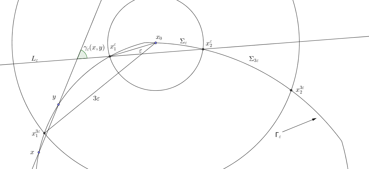
Figure 1.

We point out some simple remarks:

• Thanks to Theorem 3.1 we have that the optimal measure $f$ satisfies $f\in L^{p}(\partial E)$ for some $p=p(E)>2$.

• If $E$ is a convex body then $\gamma_{\varepsilon}$ is bounded away from $\frac{\pi}{2}$ and $|x_{1}^{3\varepsilon}-x_{1}^{\varepsilon}|\sim|x_{2}^{3\varepsilon}-x_{2}^{\varepsilon}|\sim\varepsilon$.

• The quantities $\Delta V$, $\Delta P$ and $\Delta\mathcal{I}_{0}$ are nonnegative by definition.

• All the constants involved up to now depend only on the Lipschitz character of $\partial E$. In particular, if $E_{n}$ is a sequence of convex bodies converging to a convex body $E$, then these constants depend only on the geometry of $E$.

Before stating the main result of this section, we prove two regularity lemmas.

Lemma 4.2.

Let $0<\beta\leq 1$ and $C,\varepsilon_{0}>0$ be given. Then, every convex body $E$ such that for every $x_{0}\in\partial E$ and every $\varepsilon\leq\varepsilon_{0}$,

$$\Delta V\leq C\varepsilon^{2+\beta}$$ (4.2)

is $C^{1,\beta}$ with $C^{1,\beta}-$norm depending only on the Lipschitz character of $\partial E$, $\varepsilon_{0}$ and $C$.

Proof.

Let $x_{0}\in\partial E$ be fixed. Since $E$ is convex, there exist $R>0$ and a convex function $u:I\to\mathbb{R}$ such that $\partial E\cap B_{R}(x_{0})=\{(t,u(t))\ :\ t\in I\}$ for some interval $I\subset\mathbb{R}$. Furthermore, $\|u^{\prime}\|_{L^{\infty}}\lesssim 1$. Let $\bar{x}\in\partial E\cap B_{R}(x_{0})$. Without loss of generality, we can assume that $\bar{x}=0=(0,u(0))$. By convexity of $u$, up to adding a linear function, we can further assume that $u\geq 0$ in $I$. Thanks to the Lipschitz bound on $u$, for $x=(t,u(t))\in\partial E\cap B_{R}(x_{0})$, we have

$$|x|=(t^{2}+|u(t)|^{2})^{1/2}\sim t.$$ (4.3)

Let now $\varepsilon>0$. For $\delta>0$, let $-1\ll t_{1}^{\delta}<0<t_{2}^{\delta}\ll 1$ such that $x_{i}^{\delta}=(t_{i}^{\delta},u(t_{i}^{\delta}))$ for $i=1,2$ (see the notation above). By (4.3), there exists $\lambda>0$ depending only on the Lipschitz character of $u$, such that $|t_{i}^{\lambda\varepsilon}|\geq\varepsilon$. Without loss of generality, we can now assume that $u(-\varepsilon)\leq u(\varepsilon)$. In particular, considering the $\Delta V$ associated to $\lambda\varepsilon$, we have that (see Figure 2)

$$\Delta V \geq 2\varepsilon u(\varepsilon)-\frac{2\varepsilon(u(\varepsilon)-u(-\varepsilon))}{2}-\int_{-\varepsilon}^{\varepsilon}u(t)\,dt$$

$$=\varepsilon(u(\varepsilon)+u(-\varepsilon))-\int_{-\varepsilon}^{\varepsilon}u(t)\,dt\,.$$

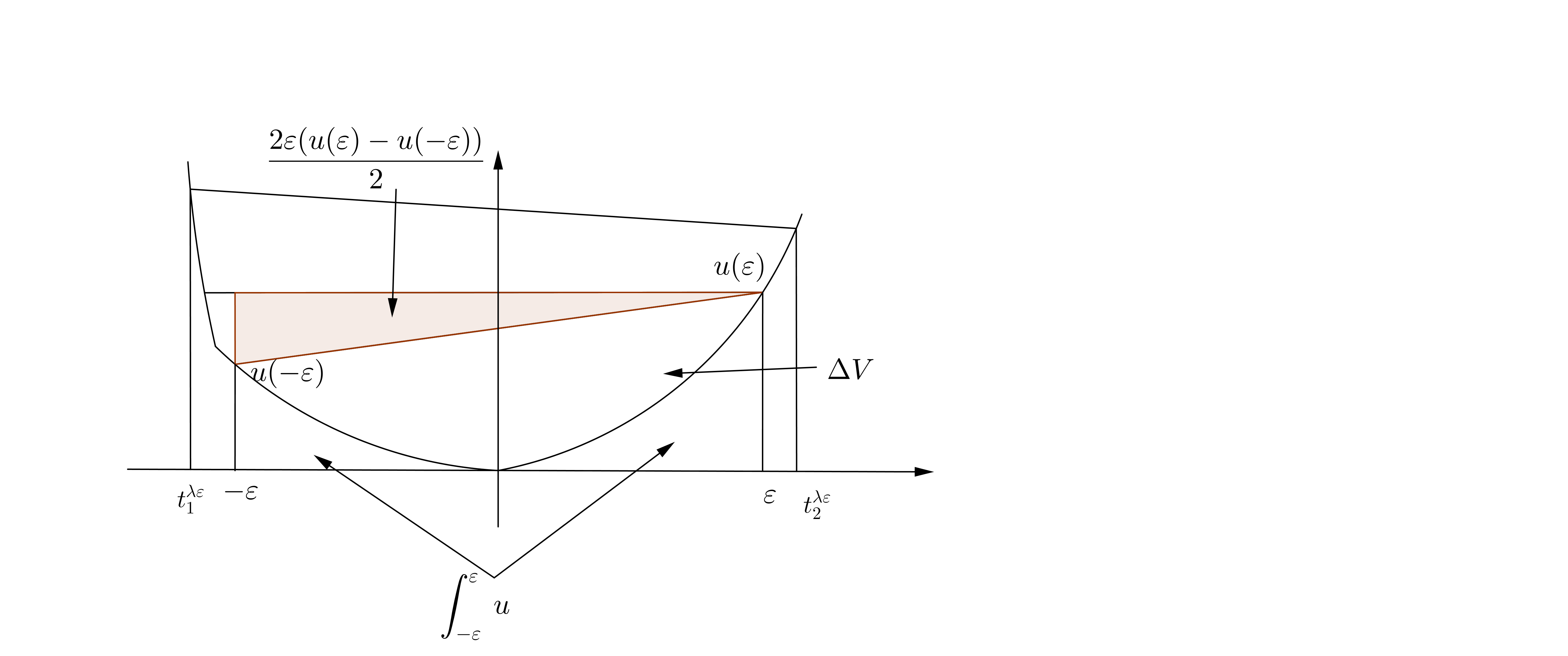
Figure 2.

Since $u$ is decreasing in $[-\varepsilon,0]$ and increasing in $[0,\varepsilon]$, this means that both

$$\varepsilon u(\varepsilon)-\int_{0}^{\varepsilon}u\lesssim\varepsilon^{2+\beta}\qquad\textrm{and }\qquad\varepsilon u(-\varepsilon)-\int^{0}_{-\varepsilon}u\lesssim\varepsilon^{2+\beta}$$ (4.4)

hold. Let us prove that this implies that for $|t|$ small enough

$$u(t)\lesssim|t|^{1+\beta}.$$ (4.5)

We can assume without loss of generality that $t>0$. By (4.4) and monotonicity of $u$,

$$tu(t)\leq Ct^{2+\beta}+\int_{0}^{t/2}u+\int_{t/2}^{t}u\leq Ct^{2+\beta}+\frac{t}{2}(u(t/2)+u(t))$$

from which we obtain

$$u(t)-u(t/2)\lesssim t^{1+\beta}.$$

Applying this for $k\geq 0$ to $t_{k}=2^{-k}t$ and summing over $k$ we obtain

$$u(t)\lesssim\sum_{k=0}^{\infty}\left(2^{-k}t\right)^{1+\beta}\lesssim t^{1+\beta},$$

that is (4.5).

In other words, we have proven that $u$ is differentiable in zero with $u^{\prime}(0)=0$ and that for $|t|$ small enough,

$$|u(t)-u(0)-u^{\prime}(0)t|\lesssim|t|^{1+\beta}.$$

Since the point zero was arbitrarily chosen, this yields that $u$ is differentiable everywhere and that for $t,s\in I$ with $|t-s|$ small enough,

$$|u(t)-u(s)-u^{\prime}(s)(t-s)|\lesssim|t-s|^{\beta+1},$$

which is equivalent to the $C^{1,\beta}$ regularity of $\partial E$.

∎

Lemma 4.3.

Suppose that the minimizer $E$ for (4.1) has boundary of class $C^{1,\beta}$, for some $0<\beta<1$. Then, there exists $R>0$ (depending only on the $C^{1,\beta}$ character of $\partial E$) such that for every $x_{0}\in\partial E$, $x\in\Sigma_{\varepsilon}$ and $y\in B_{R}(x_{0})$,

$$\gamma_{\varepsilon}(x,y)\lesssim\varepsilon^{\beta}+|x-y|^{\beta}.$$ (4.6)

Proof.

Without loss of generality, we can assume that $x_{0}=0$. As in the proof of Lemma 4.2, since $E$ is convex and of class $C^{1,\beta}$, in the ball $B_{R}(0)$, for a small enough $R$, $\partial E$ is a graph over its tangent of a $C^{1,\beta}$ function $u$. Up to a rotation, we can further assume that this tangent is horizontal so that for some interval $I\subset\mathbb{R}$, we have $\partial E\cap B_{R}(0)=\{(t,u(t))\ :\ t\in I\}$. In particular, if $x=(t,u(t))\in\partial E\cap B_{R}(0)$, $|u(t)|\lesssim|t|^{1+\beta}$ and $|u^{\prime}(t)|\lesssim|t|^{\beta}$.
For $x=(t,u(t))\in\Sigma_{\varepsilon}$ and $y=(s,u(s))\in B_{R}(0)$, let $\tilde{\gamma}_{\varepsilon}(x,y)$ be the angle between $L_{x,y}$ and the horizontal line, i.e., $\tan(\tilde{\gamma}_{\varepsilon}(x,y))=\frac{|u(t)-u(s)|}{|t-s|}$. Let us begin by estimating $\tilde{\gamma}_{\varepsilon}$. First, if $|x-y|\lesssim\varepsilon$ (which thanks to (4.3) amounts to $|t-s|\lesssim\varepsilon$ and thus since $x\in\Sigma_{\varepsilon}$, $|t|+|s|\lesssim\varepsilon$),

$$\tilde{\gamma}_{\varepsilon}(x,y)\sim\frac{|u(t)-u(s)|}{|t-s|}\leq\sup_{r\in[s,t]}|u^{\prime}(r)|\lesssim\varepsilon^{\beta}.$$

Otherwise, if $|x-y|\gg\varepsilon$, since $|x|\lesssim\varepsilon$, we have $|x-y|\sim|y|\sim|s|$ and thus

$$\tilde{\gamma}_{\varepsilon}(x,y)\lesssim\frac{|u(t)|+|u(s)|}{|t-s|}\lesssim\frac{\varepsilon^{1+\beta}+|s|^{1+\beta}}{|s|}\lesssim|s|^{\beta}\lesssim|x-y|^{\beta}.$$

Putting these estimates together, we find

$$\tilde{\gamma}_{\varepsilon}(x,y)\lesssim\varepsilon^{\beta}+|x-y|^{\beta}.$$ (4.7)

Let $\xi_{\varepsilon}$ be the angle between $L_{\varepsilon}$ and the horizontal line (see Figure 3). Since $\gamma_{\varepsilon}(x,y)=\tilde{\gamma}_{\varepsilon}\pm\xi_{\varepsilon}$, (4.6) holds provided that we can show

$$\xi_{\varepsilon}\lesssim\varepsilon^{\beta}.$$ (4.8)

Let $t_{1}^{\varepsilon},t_{2}^{\varepsilon}\sim\varepsilon$ be such that $x_{1}^{\varepsilon}=(-t_{1}^{\varepsilon},u(-t_{1}^{\varepsilon}))$ and $x_{2}^{\varepsilon}=(t_{2}^{\varepsilon},u(t_{2}^{\varepsilon}))$. We see that $\xi_{\varepsilon}$ is maximal if $u(-t_{1}^{\varepsilon})=0$, and then $t_{1}^{\varepsilon}=\varepsilon$. In that case, $\tan\xi_{\varepsilon}=\frac{u(t_{2}^{\varepsilon})}{\varepsilon+t_{2}^{\varepsilon}}$.

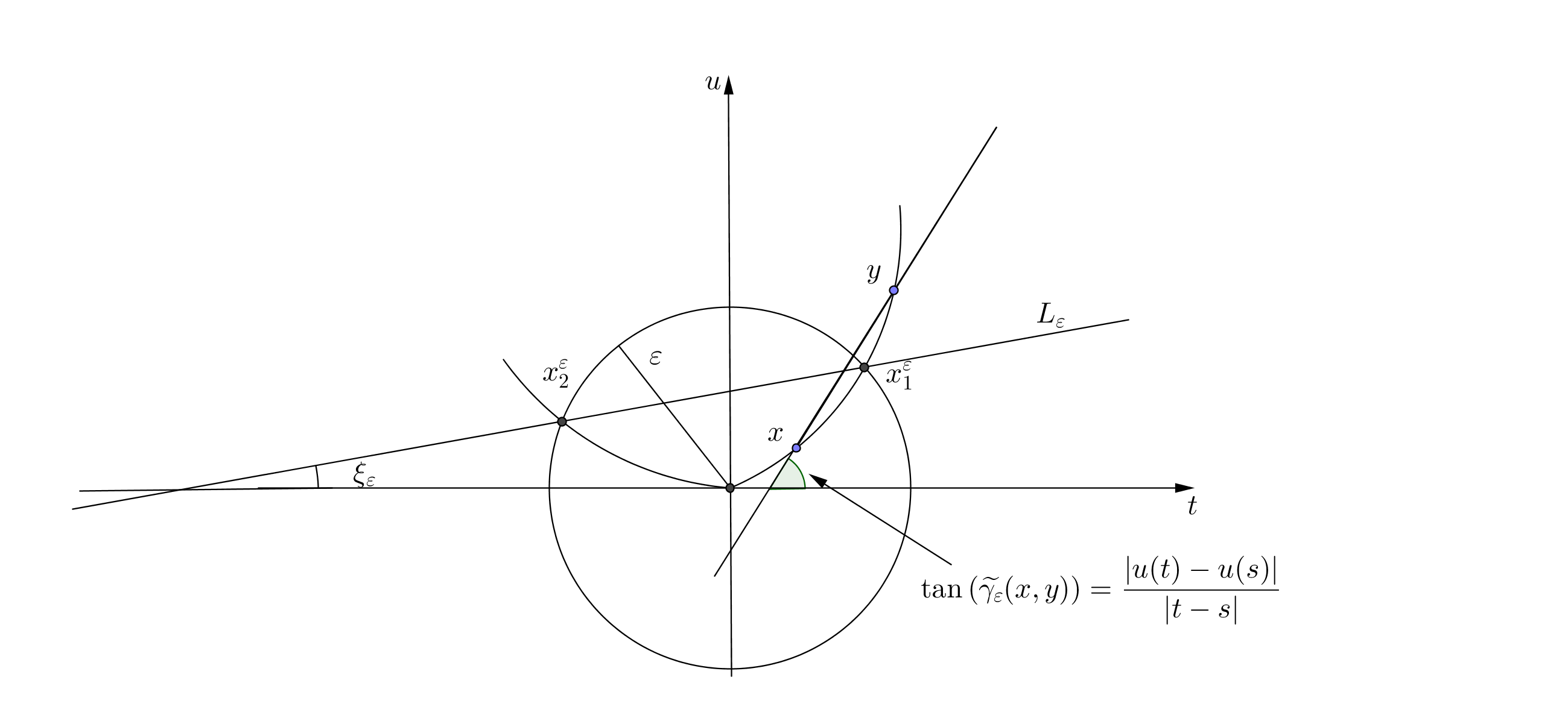
Figure 3.

Since $u(t_{2}^{\varepsilon})\lesssim\varepsilon^{1+\beta}$, and $t^{2}_{\varepsilon}\lesssim\varepsilon$, we obtain

$$\xi_{\varepsilon}\sim\tan\xi_{\varepsilon}\lesssim\frac{\varepsilon^{1+\beta}}{\varepsilon}=\varepsilon^{\beta},$$

proving (4.8). This concludes the proof of (4.6). ∎

We pass now to the main result of this section.

Theorem 4.4.

Every minimizer of (4.1) is $C^{1,1}$. Moreover, for every $Q_{0}$ and every $Q\leq Q_{0}$, the $C^{1,1}$ character of $\partial E$ depends only on $Q_{0}$, the Lipschitz character of $\partial E$ and $\|f\|_{L^{p}(\partial E)}$.

Proof.

Let $E$ be a minimizer of (4.1), $x_{0}\in\partial E$ be fixed and let $\varepsilon\leq\varepsilon_{0}$. With the above notation in force, we begin by observing that using $E_{\varepsilon}$ as a competitor, by minimality of $E$ for (4.1), we have

$$Q^{2}\Delta\mathcal{I}_{0}\geq\Delta P-\Lambda\Delta V.$$ (4.9)

We are thus going to estimate $\Delta\mathcal{I}_{0}$, $\Delta P$ and $\Delta V$ in terms of $\varepsilon$ and $\gamma_{\varepsilon}$. This will give us a quantitative decay estimate for $\gamma_{\varepsilon}$. This in turn, in light of (4.10) below and Lemma 4.2, will provide the desired regularity of $E$.

Step 1 (Volume estimate): In this first step, we prove that

$$\Delta V\sim\varepsilon^{2}\gamma_{\varepsilon}\,.$$ (4.10)

By construction, we have $\Delta V=|E|-|E_{\varepsilon}|=|E\cap H_{\varepsilon}^{+}|$. By convexity, we first have that the triangle with vertices $x_{0},x_{1}^{\varepsilon},x_{2}^{\varepsilon}$ is contained inside $E\cap H_{\varepsilon}^{+}$. By convexity again, letting ${\bar{x}_{1}}^{\varepsilon}$ be the point of $\partial B_{\varepsilon}(x_{0})$ diametrically opposed to $x_{1}^{\varepsilon}$ (and similarly for ${\bar{x}_{2}}^{\varepsilon}$), we get that $E\cap H_{\varepsilon}^{+}$ is contained in the union of the triangles of vertices $x_{2}^{\varepsilon},x_{1}^{\varepsilon},{\bar{x}_{1}}^{\varepsilon}$ and $x_{1}^{\varepsilon},x_{1}^{\varepsilon},{\bar{x}_{2}}^{\varepsilon}$ (see Figure 4).

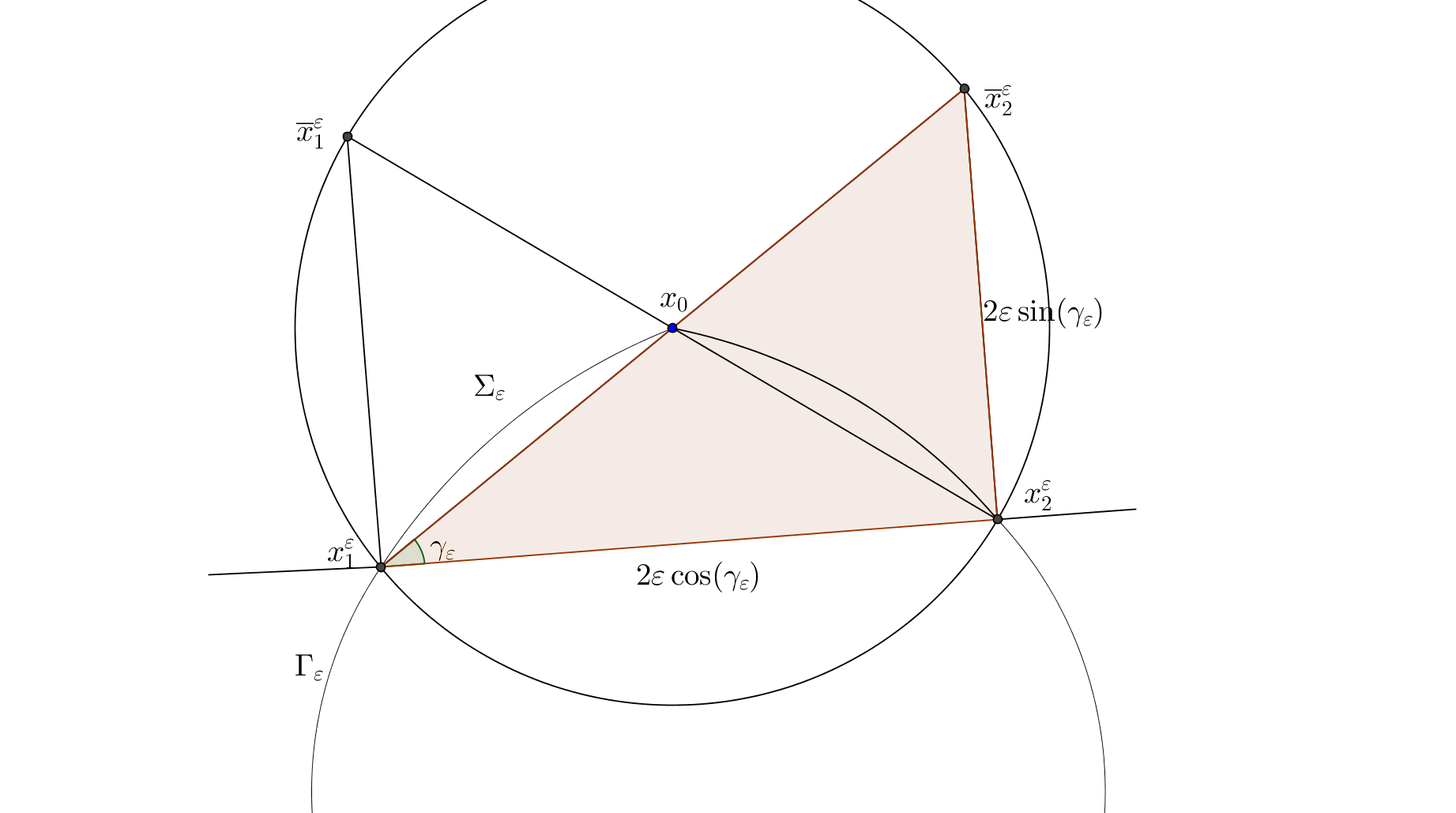
Figure 4. $\Delta V$ is contained in the union of the triangles of vertices $x_{1}^{\varepsilon},x_{2}^{\varepsilon},{\bar{x}_{1}}^{\varepsilon}$ and $x_{1}^{\varepsilon},x_{2}^{\varepsilon},{\bar{x}_{2}}^{\varepsilon}$.

Therefore, we obtain

$$\Delta V\sim\ \varepsilon^{2}\cos\gamma_{\varepsilon}\sin\gamma_{\varepsilon}\sim\varepsilon^{2}\gamma_{\varepsilon}.$$

Step 2 (Perimeter estimate): Since the triangle with vertices $x_{0},x_{1}^{\varepsilon},x_{2}^{\varepsilon}$ is contained inside $E\cap H_{\varepsilon}^{+}$, it holds

$$\Delta P=P(E)-P(E_{\varepsilon})\geq 2\varepsilon\left(1-\cos\gamma_{\varepsilon}\right)\gtrsim\varepsilon\gamma_{\varepsilon}^{2}.$$ (4.11)

Step 3 (Non-local energy estimate): We now estimate $\Delta\mathcal{I}_{0}$. Since $\mu_{\varepsilon}$ is a competitor for $\mathcal{I}_{0}(E_{\varepsilon})$, recalling that $\Pi$ is the identity outside $\Sigma_{\varepsilon}$, we have

$$\Delta\mathcal{I}_{0} =\mathcal{I}_{0}(E_{\varepsilon})-\mathcal{I}_{0}(E)$$

$$\leq\int_{\partial E_{\varepsilon}\times\partial E_{\varepsilon}}f_{\varepsilon}(x)f_{\varepsilon}(y)\log\left(\frac{1}{|x-y|}\right)-\int_{\partial E\times\partial E}f(x)f(y)\log\left(\frac{1}{|x-y|}\right)$$

$$=\int_{\partial E\times\partial E}f(x)f(y)\log\left(\frac{1}{|\Pi(x)-\Pi(y)|}\right)-\int_{\partial E\times\partial E}f(x)f(y)\log\left(\frac{1}{|x-y|}\right)$$

$$=\int_{\partial E\times\partial E}f(x)f(y)\log\left(\frac{|x-y|}{|\Pi(x)-\Pi(y)|}\right).$$

Since for $x,y\in\Sigma_{\varepsilon}^{c}$, $|\Pi(x)-\Pi(y)|=|x-y|$,

$$\Delta\mathcal{I}_{0} \leq\int_{{\Sigma_{3\varepsilon}}\times{\Sigma_{3\varepsilon}}}f(x)f(y)\log\left(\frac{|x-y|}{|\Pi(x)-\Pi(y)|}\right)$$

$$+2\int_{\Sigma_{\varepsilon}}\int_{\Gamma_{\varepsilon}}f(x)f(y)\log\left(\frac{|x-y|}{|\Pi(x)-y|}\right)$$

$$=:I_{1}+2I_{2}.$$

We first estimate $I_{1}$:

$$I_{1} =\int_{{\Sigma_{3\varepsilon}}\times{\Sigma_{3\varepsilon}}}f(x)f(y)\log\left(1+\frac{|x-y|-|\Pi(x)-\Pi(y)|}{|\Pi(x)-\Pi(y)|}\right)$$

$$\leq\int_{{\Sigma_{3\varepsilon}}\times{\Sigma_{3\varepsilon}}}f(x)f(y)\frac{|x-y|-|\Pi(x)-\Pi(y)|}{|\Pi(x)-\Pi(y)|}.$$

Since for any $x,y\in{\Sigma_{3\varepsilon}}$ we have (with equality if $x,y\in\Sigma_{\varepsilon}$),

$$\cos(\gamma_{\varepsilon}(x,y))|x-y|\leq|\Pi(x)-\Pi(y)|,$$

we get

$$I_{1}\leq\int_{{\Sigma_{3\varepsilon}}\times{\Sigma_{3\varepsilon}}}f(x)f(y)\left(\frac{1}{\cos(\gamma_{\varepsilon}(x,y))}-1\right)\lesssim\int_{{\Sigma_{3\varepsilon}}\times{\Sigma_{3\varepsilon}}}\gamma_{\varepsilon}^{2}(x,y)f(x)f(y).$$ (4.12)

Using then Hölder’s inequality (recall that $f\in L^{p}(\partial E)$ for some $p>2$) to get

$$\int_{{\Sigma_{3\varepsilon}}}f\leq\left(\int_{{\Sigma_{3\varepsilon}}}f^{p}\right)^{1/p}\mathcal{H}^{1}({\Sigma_{3\varepsilon}})^{\frac{p-1}{p}}\lesssim\varepsilon^{\frac{p-1}{p}},$$ (4.13)

and $\gamma_{\varepsilon}(x,y)\lesssim 1$, we obtain

$$I_{1}\lesssim\varepsilon^{2\frac{p-1}{p}}.$$ (4.14)

We can now estimate $I_{2}$:

$$I_{2} =\int_{\Sigma_{\varepsilon}}\int_{\Gamma_{\varepsilon}}f(x)f(y)\log\left(1+\left(\frac{|x-y|-|\Pi(x)-y|}{|\Pi(x)-y|}\right)\right)$$

$$\leq\int_{\Sigma_{\varepsilon}}\int_{\Gamma_{\varepsilon}}f(x)f(y)\left(\frac{|x-y|-|\Pi(x)-y|}{|\Pi(x)-y|}\right).$$

Denote by $z$ the projection of $\Pi(x)$ on the line containing $x$ and $y$. Then, since the projection is a $1$-Lipschitz function, it holds $|z-y|\leq|\Pi(x)-y|$. Thus,

$$|x-y|-|y-\Pi(x)|=|x-z|+|z-y|-|y-\Pi(x)|\leq|x-z|.$$

Arguing as in Step 1, we get $|x-\Pi(x)|\leq|\overline{x}_{2}^{\varepsilon}-x_{2}^{\varepsilon}|\lesssim\varepsilon\gamma_{\varepsilon}$. Furthermore, the angle $\widehat{z\Pi(x)x}$ equals $\gamma_{\varepsilon}(x,y)$ (see Figure 5), so that

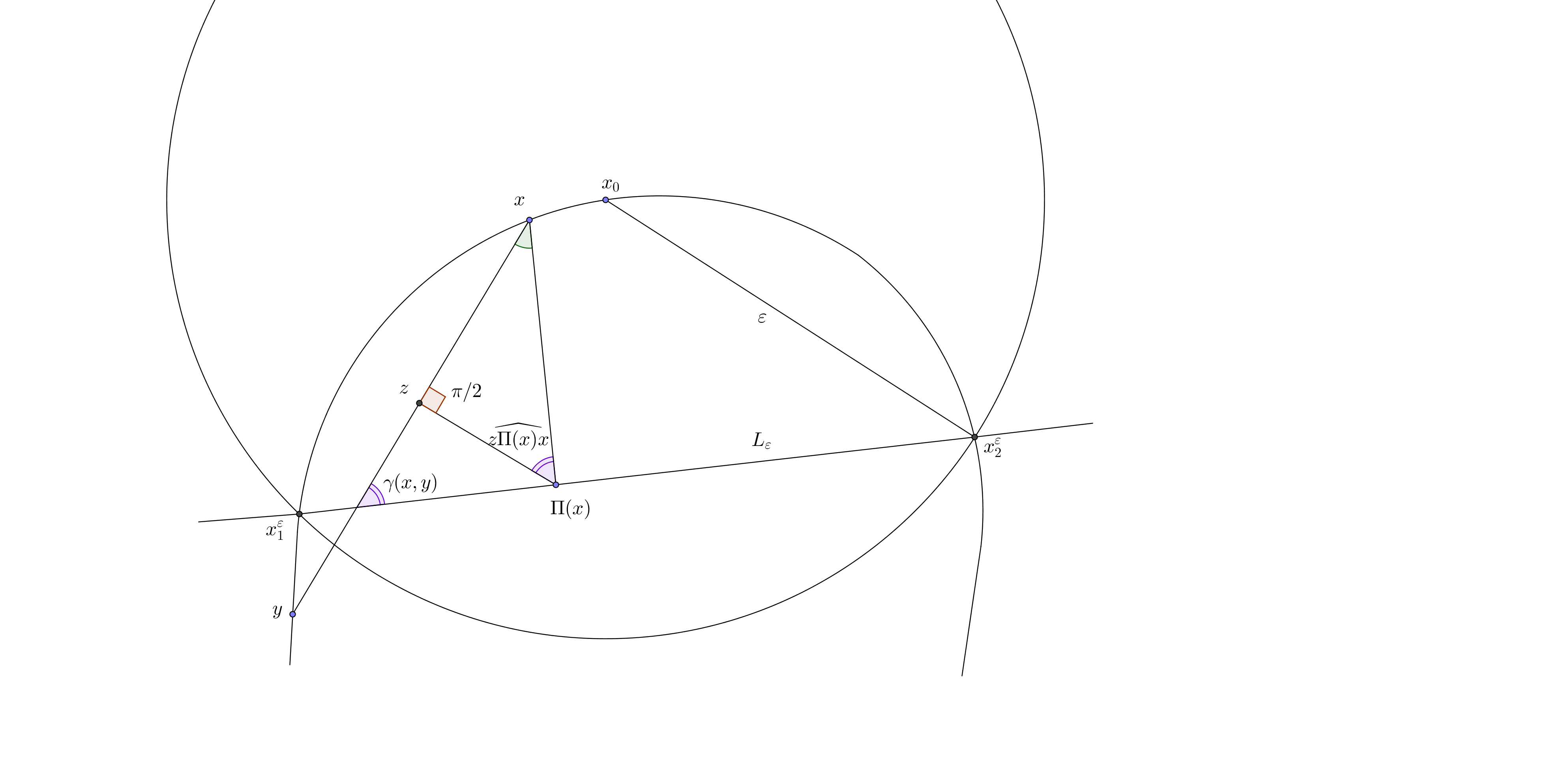
Figure 5. The angle $\widehat{z\Pi(x)x}$ equals $\gamma(x,y)$.

$$|x-y|-|y-\Pi(x)|\leq|x-z|=|x-\Pi(x)|\sin(\gamma_{\varepsilon}(x,y))\lesssim\varepsilon\gamma_{\varepsilon}\gamma_{\varepsilon}(x,y).$$

On the other hand, since $|y-x|\geq 2\varepsilon$ (indeed $|x-x_{0}|\leq\varepsilon$ and $|y-x_{0}|\geq 3\varepsilon$), we have

$$|y-\Pi(x)|\geq|y-x|-|x-\Pi(x)|\gtrsim|y-x|-\varepsilon\gtrsim|y-x|.$$

Therefore,

$$I_{2}\lesssim\varepsilon\gamma_{\varepsilon}\int_{\Sigma_{\varepsilon}}\int_{\Gamma_{\varepsilon}}\frac{f(x)f(y)\gamma_{\varepsilon}(x,y)}{|y-x|}.$$ (4.15)

There exists $M>0$ which depends only on the Lipschitz character of $\partial E$ such that for $x\in\Sigma_{\varepsilon}$ and $y\in\Gamma_{\varepsilon}\cap B_{M}(x_{0})$,

$$|y-x|\geq\min_{i=1,2}|y-{x}_{i}^{\varepsilon}|.$$

Let $\Gamma_{\varepsilon}^{N}:=\Gamma_{\varepsilon}\cap B_{M}(x_{0})$ and $\Gamma_{\varepsilon}^{F}:=\Gamma_{\varepsilon}\cap B^{c}_{M}(x_{0})$. We then have

$$I_{2} \lesssim\varepsilon\gamma_{\varepsilon}\left(\int_{\Sigma_{\varepsilon}\times\Gamma_{\varepsilon}^{N}}\frac{f(x)f(y)\gamma_{\varepsilon}(x,y)}{\min_{i}|y-{x}_{i}^{\varepsilon}|}+\int_{\Sigma_{\varepsilon}\times\Gamma_{\varepsilon}^{F}}f(x)f(y)\gamma_{\varepsilon}(x,y)\right)$$

$$=:I_{2}^{N}+I_{2}^{F}.$$

We begin by estimating $I_{2}^{F}$. Since $\gamma_{\varepsilon}(x,y)\lesssim 1$, using Hölder’s inequality we find

$$I_{2}^{F} \lesssim\varepsilon\gamma_{\varepsilon}\left(\int_{\Gamma_{\varepsilon}}f\right)\left(\int_{\Sigma_{\varepsilon}}f\right)$$ (4.16)

$$\leq\varepsilon\gamma_{\varepsilon}\|f\|_{L^{p}}\mathcal{H}^{1}(\Gamma_{\varepsilon})^{1-\frac{1}{p}}\|f\|_{L^{p}}\mathcal{H}^{1}(\Sigma_{\varepsilon})^{1-\frac{1}{p}}$$

$$\lesssim\varepsilon\gamma_{\varepsilon}\mathcal{H}^{1}(\Sigma_{\varepsilon})^{1-\frac{1}{p}}$$

$$\lesssim\varepsilon^{2-\frac{1}{p}}\gamma_{\varepsilon}.$$

We can now estimate $I_{2}^{N}$. Recall that

$$I_{2}^{N}:=\varepsilon\gamma_{\varepsilon}\int_{\Sigma_{\varepsilon}\times\Gamma_{\varepsilon}^{N}}\frac{f(x)f(y)\gamma_{\varepsilon}(x,y)}{\min_{i}|y-{x}_{i}^{\varepsilon}|}.$$ (4.17)

As before, we use $\gamma_{\varepsilon}(x,y)\lesssim 1$ together with Hölder’s inequality applied twice to get

$$\int_{\Sigma_{\varepsilon}\times\Gamma_{\varepsilon}^{N}}\frac{f(x)f(y)\gamma_{\varepsilon}(x,y)}{\min_{i}|y-{x}_{i}^{\varepsilon}|}\lesssim\varepsilon^{1-1/p}\left(\int_{\Gamma_{\varepsilon}^{N}}\frac{1}{\min_{i}|y-{x}_{i}^{\varepsilon}|^{p/(p-1)}}\right)^{(p-1)/p}.$$

Since $E$ is convex, its boundary can be locally parametrized by Lipschitz functions so that, if $M$ is small enough (depending only on the Lipschitz regularity of $\partial E$), then for $y\in\Gamma_{\varepsilon}^{N}$, $\min_{i}\ell(y,\tilde{x}_{i}^{\varepsilon})\sim\min_{i}|y-\tilde{x}_{i}^{\varepsilon}|$ (where $\ell(x,y)$ denotes the geodesic distance on $\partial E$). From this we get

$$\int_{\Gamma_{\varepsilon}^{N}}\frac{1}{\min_{i}|y-{x}_{i}^{\varepsilon}|^{p/(p-1)}}\lesssim\varepsilon^{-1/(p-1)}.$$

From this we conclude that

$$I_{2}^{N}\lesssim\gamma_{\varepsilon}\varepsilon^{2-\frac{2}{p}}.$$ (4.18)

Step 4 ($C^{1,\beta}$ regularity): We now prove that $E$ has boundary of class $C^{1,\beta}$. To this aim, we can assume that $\Delta V\ll\Delta P$. Indeed, if $\Delta V\gtrsim\Delta P$, thanks to (4.10) and (4.11), we would get $\gamma_{\varepsilon}\lesssim\varepsilon$ and thus $\Delta V\lesssim\varepsilon^{3}$, which by Lemma 4.2 would already ensure the $C^{1,1}$ regularity of $\partial E$. Using (4.9), (4.11), (4.14), (4.16) and (4.18), we get

$$Q^{2}(\varepsilon^{1-\frac{2}{p}}+\gamma_{\varepsilon}(\varepsilon^{1-\frac{1}{p}}+\varepsilon^{1-\frac{2}{p}}))\gtrsim\gamma_{\varepsilon}^{2}.$$ (4.19)

Now since $\varepsilon^{1-\frac{1}{p}}\lesssim\varepsilon^{1-\frac{2}{p}}$, this reduces further to

$$Q^{2}(\varepsilon^{1-\frac{2}{p}}+\gamma_{\varepsilon}\varepsilon^{1-\frac{2}{p}})\gtrsim\gamma_{\varepsilon}^{2}.$$ (4.20)

We can now distinguish two cases. Either $Q^{2}\varepsilon^{2(\frac{1}{2}-\frac{1}{p})}\gtrsim\gamma_{\varepsilon}^{2}$ and then $\gamma_{\varepsilon}\lesssim Q\varepsilon^{(\frac{1}{2}-\frac{1}{p})}$ or $Q^{2}\gamma_{\varepsilon}\varepsilon^{1-\frac{2}{p}}\gtrsim\gamma_{\varepsilon}^{2}$ and then $\gamma_{\varepsilon}\lesssim Q^{2}\varepsilon^{1-\frac{2}{p}}$. Thus in both cases, since $p>2$, we find $\gamma_{\varepsilon}\lesssim Q\varepsilon^{\beta}$ for some $\beta>0$ and we can conclude, by means of (4.10) and Lemma 4.2, that $\partial E$ is $C^{1,\beta}$.

Step 5 ($C^{1,1}$ regularity): Thanks to Lemma 3.6, we get that $f\in L^{\infty}$ with $\|f\|_{L^{\infty}}$ depending only on the Lipschitz character of $\partial E$ and on $\|f\|_{L^{p}}$. Using this new information, we can improve (4.14), (4.16) and (4.18) to

$$I_{1}\lesssim\varepsilon^{2},\quad I_{2}^{F}\lesssim\gamma_{\varepsilon}\varepsilon^{2},\quad\textrm{and}\quad I_{2}^{N}\lesssim\gamma_{\varepsilon}\varepsilon^{2}|\log\varepsilon|.$$ (4.21)

Arguing as in Step 4, we find $\gamma_{\varepsilon}\lesssim Q\varepsilon^{1/2}$ and thus $\partial E$ is of class $C^{1,1/2}$. In order to get higher regularity, we need to get a better estimate on $\gamma_{\varepsilon}(x,y)$.

Going back to (4.12) and using (4.6) with $\beta=1/2$, we find the improved estimate

$$I_{1}\lesssim\varepsilon^{3}.$$ (4.22)

If we also use (4.6) in (4.17), we obtain

$$I_{2}^{N} \lesssim\varepsilon\gamma_{\varepsilon}\int_{\Sigma_{\varepsilon}\times\Gamma^{N}_{\varepsilon}}\frac{\varepsilon^{1/2}+|x-y|^{1/2}}{\min_{i}|y-\tilde{x}_{i}^{\varepsilon}|}$$

$$\lesssim\varepsilon\gamma_{\varepsilon}\int_{\Sigma_{\varepsilon}\times\Gamma^{N}_{\varepsilon}}\frac{\varepsilon^{1/2}+\min_{i}\{|x-\tilde{x}_{i}^{\varepsilon}|^{1/2}+|y-\tilde{x}_{i}^{\varepsilon}|^{1/2}\}}{\min_{i}|y-\tilde{x}_{i}^{\varepsilon}|}$$

$$\lesssim\varepsilon\gamma_{\varepsilon}\int_{\Sigma_{\varepsilon}\times\Gamma^{N}_{\varepsilon}}\frac{\varepsilon^{1/2}+\min_{i}|y-\tilde{x}_{i}^{\varepsilon}|^{1/2}}{\min_{i}|y-\tilde{x}_{i}^{\varepsilon}|}$$

$$\lesssim\varepsilon^{2}\gamma_{\varepsilon}\int_{\Gamma^{N}_{\varepsilon}}\frac{\varepsilon^{1/2}}{\min_{i}|y-\tilde{x}_{i}^{\varepsilon}|}+\frac{1}{\min_{i}|y-\tilde{x}_{i}^{\varepsilon}|^{1/2}}$$

$$\lesssim\varepsilon^{2}\gamma_{\varepsilon}(\varepsilon^{1/2}|\log\varepsilon|+1)\lesssim\varepsilon^{2}\gamma_{\varepsilon}.$$

As in the beginning of Step 4, we can assume that $\Delta V\ll\Delta P$, so that by (4.9) and (4.11) we have $Q^{2}\Delta\mathcal{I}_{0}\gtrsim\Delta P\gtrsim\varepsilon\gamma_{\varepsilon}^{2}$. By the previous estimate for $I_{2}^{N}$, (4.22) and the second inequality in (4.21) we eventually get

$$Q^{2}\varepsilon^{2}\gamma_{\varepsilon}\sim Q^{2}(\varepsilon^{3}+\varepsilon^{2}\gamma_{\varepsilon})\gtrsim\varepsilon\gamma_{\varepsilon}^{2},$$

which leads to $\gamma_{\varepsilon}\lesssim Q^{2}\varepsilon$. By using again Lemma 4.2, the proof is concluded. ∎

5. Minimality of the ball for $N=2$ and $Q$ small

We now use the regularity result obtained in Section 4 to prove that for small charges, the only minimizers of $\mathcal{F}_{Q,0}$ in dimension two are balls.

Theorem 5.1.

Let $N=2$ and $\alpha=0$. There exists $Q_{0}>0$ such that for $Q<Q_{0}$, up to translations, the only minimizer of (1.1) is the ball.

Proof.

Let $E_{Q}$ be a minimizer of $\mathcal{F}_{Q,0}$ and let $B$ be a ball of measure one. By minimality of $E_{Q}$, we have

$$P(E_{Q})-P(B)\leq Q^{2}\left(\mathcal{I}_{0}(B)-\mathcal{I}_{0}(E_{Q})\right)\leq Q^{2}\left(\mathcal{I}_{0}(B)+|\mathcal{I}_{0}(E_{Q})|\right).$$ (5.1)

By Lemma 4.1 the diameter of $E_{Q}$ is uniformly bounded and so is $|\mathcal{I}_{0}(E_{Q})|$. Using the quantitative isoperimetric inequality (see [8]), we infer

$$|E_{Q}\Delta B|^{2}\lesssim P(E_{Q})-P(B)\leq Q^{2}\left(\mathcal{I}_{0}(B)+|\mathcal{I}_{0}(E_{Q})|\right).$$

This implies that $E_{Q}$ converges to $B$ in $L^{1}$ as $Q\to 0$. From the convexity of $E_{Q}$, this implies the convergence also in the Hausdorff metric. Since the sets $E_{Q}$ are all uniformly bounded and of fixed volume, they are uniformly Lipschitz. Theorem 4.4 then implies that $\partial E_{Q}$ are $C^{1,1}-$regular sets with $C^{1,1}$ norm uniformly bounded. Therefore, thanks to the Arzelà-Ascoli’s Theorem, we can write

$$\partial E_{Q}=\left\{(1+\varphi_{Q}(x))x:\,x\in\partial B\right\},$$

with $\|\varphi_{Q}\|_{C^{1,\beta}}$ converging to $0$ as $Q\to 0$ for every $\beta<1$. From Lemma 3.6 we infer that the optimal measures $\mu_{Q}$ for $E_{Q}$ are uniformly $C^{0,\beta}$ and in particular are uniformly bounded. Using now [11, Proposition 6.3], we get that for small enough $Q$,

$$\|\mu_{Q}\|_{L^{\infty}}^{2}\left(P(E_{Q})-P(B)\right)\gtrsim\mathcal{I}_{0}(B)-\mathcal{I}_{0}(E_{Q})$$

Putting this into (5.1), we then obtain

$$P(E_{Q})-P(B)\lesssim Q^{2}(P(E_{Q})-P(B))$$

from which we deduce that for $Q$ small enough, $P(E_{Q})=P(B)$. Since, up to translations, the ball is the unique solution of the isoperimetric problem, this implies $E_{Q}=B$. ∎

6. Asymptotic behavior as $Q\to+\infty$

In this section we characterize the limit shape of (suitably rescaled) minimizers of $\mathcal{F}_{Q,\alpha}$, with $\alpha\in[0,1]$, as the charge $Q$ tends to $+\infty$. For this, we fix a sequence $Q_{n}\to+\infty$.

6.1. The case $\alpha\in[0,1)$

For $n\in\mathbb{N}$, we let $V_{n}:=Q_{n}^{-\frac{2N(N-1)}{1+(N-1)\alpha}}$ (so that $V_{n}\to 0$ as $n\to+\infty$) and

$$\mathcal{A}_{n,\alpha} := \left\{E\subset\mathbb{R}^{N}\ \text{convex body,}\ |E|=V_{n}\right\},$$

$$\widehat{\mathcal{F}}_{n,\alpha}(E) := V_{n}^{-\frac{N-2}{N-1}}P(E)+\mathcal{I}_{\alpha}(E)\qquad\textrm{ for }E\in\mathcal{A}_{n,\alpha}.$$

It is straightforward to check that if $E$ is a minimizer of (1.1), then the rescaled set

$$\widehat{E}:=Q_{n}^{-\frac{2(N-1)}{1+(N-1)\alpha}}\,E$$

is a minimizer of $\widehat{\mathcal{F}}_{n,\alpha}$ in the class $\mathcal{A}_{n,\alpha}$.

We begin with a compactness result for a sequence of sets of equibounded energy.

Proposition 6.1.

Let $\alpha\in[0,1)$ and let $E_{n}\in\mathcal{A}_{n,\alpha}$ be such that

$$\sup_{n}\widehat{\mathcal{F}}_{n,\alpha}(E_{n})<+\infty.$$

Then, up to extracting a subsequence and up to rigid motions, the sets $E_{n}$ converge in the Hausdorff topology to the segment $[0,L]\times\{0\}^{N-1}$, for some $L\in(0,+\infty)$.

Proof.

The bound on $\mathcal{I}_{\alpha}(E_{n})$ directly implies with (2.2) (or (2.3) in the case $\alpha=0$) that the diameter of $E_{n}$ is uniformly bounded from below.

Let us show that the diameter of $E_{n}$ is also uniformly bounded from above. Arguing as in Theorem 2.3, let $\mathcal{R}_{n}=\prod_{i=1}^{N}[0,\lambda_{i}^{n}]$ be the parallelepipeds given by Lemma 2.2, and assume without loss of generality that $\lambda_{1}^{n}\geq\lambda_{2}^{n}\geq\dots\geq\lambda_{N}^{n}$. In the case $\alpha>0$, (2.1) directly gives the bound while for $\alpha=0$, we get using (2.1) and (2.3), that $|\mathcal{I}_{0}(\mathcal{R}_{n})|$ is uniformly bounded, from which the bound on the diameter follows, using once again (2.1). Moreover, from (2.2) and (2.3), we obtain that $\lambda_{i}^{n}\sim V_{n}^{\frac{1}{N-1}}$ (where the constants depend on $\widehat{\mathcal{F}}_{n,\alpha}(E_{n})$), for $i=2,\dots,N$. The convex bodies $E_{n}$ are therefore compact in the Hausdorff topology and any limit set is a non-trivial segment of length $L\in(0,+\infty)$. ∎

In the proof of the $\Gamma-$convergence result we will use the following result.

Lemma 6.2.

Let $0<\gamma<\beta$ with $\beta\geq 1$, $V>0$ and $L>0$, then

$$\min\left\{\int_{0}^{L}f^{\gamma}\ :\ \int_{0}^{L}f^{\beta}=V,\ f\textrm{ concave and }f\geq 0\right\}=\frac{(\beta+1)^{\gamma/\beta}}{\gamma+1}L^{1-\frac{\gamma}{\beta}}V^{\gamma/\beta}.$$ (6.1)

Proof.

For $L,V>0$, let

$$M(L,V):=\min\left\{\int_{0}^{L}f^{\gamma}\ :\ \int_{0}^{L}f^{\beta}=V,\ f\textrm{ concave and }f\geq 0\right\}.$$

Let us now prove (6.1). By scaling, we can assume that $L=V=1$. Thanks to the concavity and positivity constraints, existence of a minimizer for (6.1) follows. Let $f$ be such a minimizer. Let us prove that we can assume that $f$ is non-increasing. Notice first that by definition, it holds

$$M(1,1)=\int_{0}^{1}f^{\gamma}.$$

Up to a rearrangement, we can assume that $f$ is symmetric around the point $1/2$, so that $f$ is non-increasing in $[1/2,1]$ and

$$\int_{1/2}^{1}f^{\gamma}=\frac{1}{2}M(1,1)=M(1/2,1/2).$$

Letting finally for $x\in[0,1]$, $\hat{f}(x):=f(\frac{1}{2}(x+\frac{1}{2}))$, we have that $\hat{f}$ is non-increasing, admissible for (6.1) and

$$\int_{0}^{1}\hat{f}^{\gamma}=2\int_{1/2}^{1}f^{\gamma}=M(1,1),$$

so that $\hat{f}$ is also a minimizer for (6.1).
Assume now that $f$ is not affine in $(0,1)$. Then there is $\overline{x}>0$ such that for all $0<x\leq\overline{x}$

$$f(x)>f(0)-(f(0)-f(1))x.$$

Let $\tilde{f}:=\lambda-(\lambda-f(1))x$ with $\lambda>f(0)$ chosen so that

$$\int_{0}^{1}f^{\beta-1}\tilde{f}=\int_{0}^{1}f^{\beta}.$$ (6.2)

Now, let $g:=\tilde{f}-f$. Since $f+g=\tilde{f}$ is concave, for every $0\leq t\leq 1$, $f+tg$ is a concave function. For $\delta\in\mathbb{R}$, let $f_{t,\delta}:=f+t(g+\delta(1-x))$. Let finally $\delta_{t}$ be such that

$$\int_{0}^{1}f_{t,\delta_{t}}^{\beta}=\int_{0}^{1}f^{\beta}.$$

Thanks to (6.2) and since $\beta\geq 1$, $|\delta_{t}|=O(t)$. Since $f_{t,\delta_{t}}$ is concave, by the minimality of $f$ we get

$$\int_{0}^{1}f_{t,\delta_{t}}^{\gamma}-\int_{0}^{1}f^{\gamma}\geq 0.$$

Dividing by $t$ and taking the limit as $t$ goes to zero, we obtain

$$\int_{0}^{1}f^{\gamma-1}g\geq 0.$$

Let $z\in(0,1)$ be the unique point such that $\tilde{f}(z)=f(z)$ (so that $\tilde{f}(x)>f(x)$ for $x<z$ and $\tilde{f}(x)<f(x)$ for $x>z$). We then have,

$$0 \leq\int_{0}^{1}f^{\beta-1}\frac{\tilde{f}-f}{f^{\beta-\gamma}}$$

$$=\int_{0}^{z}f^{\beta-1}\frac{\tilde{f}-f}{f^{\beta-\gamma}}+\int_{z}^{1}f^{\beta-1}\frac{\tilde{f}-f}{f^{\beta-\gamma}}$$

$$<\frac{1}{f^{\beta-\gamma}(z)}\left(\int_{0}^{z}f^{\beta-1}(\tilde{f}-f)+\int_{z}^{1}f^{\beta-1}(\tilde{f}-f)\right)$$

$$=\frac{1}{f^{\beta-\gamma}(z)}\int_{0}^{1}f^{\beta-1}(\tilde{f}-f),$$

which contradicts (6.2).

We are left to study the case when $f$ is linear. Assume that $f(1)>0$ and let

$$\delta:=\frac{\int_{0}^{1}f^{\beta-1}}{\int_{0}^{1}xf^{\beta-1}}>1,$$

so that in particular, $\int_{0}^{1}f^{\beta-1}(1-\delta x)=0$. Up to adjusting the volume as in the previous case, for $t>0$ small enough, $f+t(1-\delta x)$ is admissible. From this, arguing as above, we find that

$$\int_{0}^{1}f^{\gamma-1}(1-\delta x)\geq 0.$$

By splitting the integral around the point $\bar{z}=\delta^{-1}\in(0,1)$ and proceeding as above, we get again a contradiction. As a consequence, we obtain that $f(x)=\lambda(1-x)$, with $\lambda=(\beta+1)^{1/\beta}$ so that the volume constraint is satisfied. This concludes the proof of (6.1). ∎

We now prove the following $\Gamma-$convergence result.

Theorem 6.3.

For $\alpha\in[0,1)$, the functionals $\widehat{\mathcal{F}}_{n,\alpha}$ $\Gamma$–converge in the Hausdorff topology, as $n\to+\infty$, to the functional

$$\widehat{\mathcal{F}}_{\alpha}(E):=\begin{cases}C_{N}\,L^{\frac{1}{N-1}}+\dfrac{\mathcal{I}_{\alpha}([0,1])}{L^{\alpha}}&\textrm{if }E\simeq[0,L]\times\{0\}^{N-1}\textrm{ and }\alpha>0\\ \\ C_{N}\,L^{\frac{1}{N-1}}+\mathcal{I}_{0}([0,1])-\log L&\textrm{if }E\simeq[0,L]\times\{0\}^{N-1}\textrm{ and }\alpha=0\\ \\ +\infty&\textrm{otherwise,}\end{cases}$$

where $E\simeq F$ means that $E=F$ up to a rigid motion, and $C_{N}:=\omega_{N-1}^{1/(N-1)}N^{(N-2)/(N-1)}$ with $\omega_{N}$ the volume of the ball of radius one in $\mathbb{R}^{N}$ (so that for $N=2$ we have $C_{2}=2$).

Proof.

By Proposition 6.1 we know that the $\Gamma$-limit is $+\infty$ on the sets which are not segments.

Let us first prove the $\Gamma$-limsup inequality. Given $L\in(0,+\infty)$, we are going to construct $E_{n}$ symmetric with respect to the hyperplane $\{0\}\times\mathbb{R}^{N-1}$. For $t\in[0,L/2]$, we let $r(t):=\left(\frac{NV_{n}}{\omega_{N-1}L}\right)^{1/(N-1)}\left(1-\frac{2t}{L}\right)$ and then

$$E_{n}\cap\left(\mathbb{R}^{+}\times\mathbb{R}^{N-1}\right):=\left\{\left(t,B_{r(t)}^{N-1}\right)\ :t\in[0,L/2]\right\},$$

where $B_{r(t)}^{N-1}$ is the ball of radius $r(t)$ in $\mathbb{R}^{N-1}$. With this definition, $|E_{n}|=V_{n}$, so that $E_{n}\in\mathcal{A}_{n,\alpha}$. We then compute

$$P(E_{n}) =2\int_{0}^{L/2}\mathcal{H}^{N-2}(\mathbb{S}^{N-2})r(t)^{N-2}\sqrt{1+|r^{\prime}|^{2}}$$

$$=2(N-1)\,\omega_{N-1}\left(\frac{NV_{n}}{\omega_{N-1}L}\right)^{\frac{N-2}{N-1}}\int_{0}^{L/2}\left(1-\frac{2t}{L}\right)^{N-2}\left(1+\frac{c_{N}}{L^{2}}\left(\frac{V_{n}}{L}\right)^{\frac{2}{N-1}}\right)^{1/2}$$

$$=C_{N}V_{n}^{\frac{N-2}{N-1}}L^{\frac{1}{N-1}}+o\left(V_{n}^{\frac{N-2}{N-1}}\right).$$

Letting $\mu_{\alpha}$ be the optimal measure for $\mathcal{I}_{\alpha}([-L/2,L/2])$, we then have

$$\widehat{\mathcal{F}}_{n,\alpha}(E_{n})\leq C_{N}L^{\frac{1}{N-1}}+\mathcal{I}_{\alpha}([0,L])+o(1),$$

which gives the $\Gamma$-limsup inequality.

We now turn to the the $\Gamma$-liminf inequality. Let $E_{n}\in\mathcal{A}_{n,\alpha}$ be such that $E_{n}\to[0,L]\times\{0\}^{N-1}$ in the Hausdorff topology. Since $\mathcal{I}_{\alpha}$ is continuous under Hausdorff convergence, it is enough to prove that

$$\liminf_{n\to+\infty}V_{n}^{-\frac{N-2}{N-1}}\,P(E_{n})\geq C_{N}\,L^{\frac{1}{N-1}}.$$ (6.3)

Let $L_{n}:=\textup{diam}(E_{n})$. By Hausdorff convergence, we have that $L_{n}\to L$. Moreover, up to a rotation and a translation, we can assume that $[0,L_{n}]\times\{0\}^{N-1}\subset E_{n}$. For $N=2$, we directly obtain $P(E_{n})\geq 2L_{n}$ which gives (6.3). We thus assume from now on that $N\geq 3$. Let $\widetilde{E}_{n}$ be the set obtained from $E_{n}$ after a Schwarz symmetrization around the axis $\mathbb{R}\times\{0\}^{N-1}$. By Brunn’s principle [3], $\widetilde{E}_{n}$ is still a convex set with $P(E_{n})\geq P(\widetilde{E}_{n})$ and $|E_{n}|=|\widetilde{E}_{n}|$. We thus have that

$$\widetilde{E}_{n}=\bigcup_{t\in[0,L_{n}]}\{t\}\times B_{r(t)}^{N-1}$$

for an appropriate function $r(t)$, and, by Fubini’s Theorem,

$$\int_{0}^{L_{N}}r(t)^{N-1}=\frac{V_{n}}{\omega_{N-1}}.$$

By the Coarea Formula [2, Theorem 2.93], we then get

$$P(\widetilde{E}_{n})\geq\mathcal{H}^{N-2}(\mathbb{S}^{N-2})\int_{0}^{L_{n}}r(t)^{N-2}\sqrt{1+|r^{\prime}(t)|^{2}}\geq\mathcal{H}^{N-2}(\mathbb{S}^{N-2})\int_{0}^{L_{n}}r(t)^{N-2}.$$

Applying then Lemma 6.2 with $\gamma=N-2$ and $\beta=N-1$, we obtain (6.3). ∎

Remark 6.4.

For $\alpha\in[0,1)$ and $N\geq 2$, it is easy to optimize $\widehat{F}_{\alpha}$ in $L$ and obtain the values $L_{N,\alpha}$ given in Theorem 1.4.

From Proposition 6.1, Theorem 6.3 and the uniqueness of the minimizers for $\widehat{F}_{\alpha}$, we directly obtain the following asymptotic result for minimizers of (1.1).

Corollary 6.5.

Let $\alpha\in[0,1)$ and $N\geq 2$. Then, up to rescalings and rigid motions, every sequence $E_{n}$ of minimizers of (1.1) converges in the Hausdorff topology to $[0,L_{N,\alpha}]\times\{0\}^{N-1}$.

6.2. The case $N=2,\,3$ and $\alpha=1$

In the case $\alpha\geq 1$, the energy $\mathcal{I}_{\alpha}$ is infinite on segments and thus a $\Gamma-$limit of the same type as the one obtained in Theorem 6.3 cannot be expected. Nevertheless in the Coulombic case $N=3$, $\alpha=1$ we can use a dual formulation of the non-local part of the energy to obtain the $\Gamma-$limit. As a by-product, we can also treat the case $N=2$, $\alpha=1$.

For $N=2,3$ and $n\in\mathbb{N}$, we let

$$\mathcal{A}_{n,1} := \left\{E\subset\mathbb{R}^{3}\ \text{convex body,}\ |E|=Q_{n}^{-2(N-1)}(\log Q_{n})^{-(N-1)}\right\}\,,$$

$$\widehat{\mathcal{F}}_{n,1}(E) := Q_{n}^{2(N-2)}(\log Q_{n})^{N-2}\,P(E)+\frac{\mathcal{I}_{1}(E)}{\log Q_{n}},\qquad\textrm{for }E\in\mathcal{A}_{n,1}\,.$$

As before, if $E$ is a minimizer of (1.1), then the rescaled set

$$\widehat{E}:=Q_{n}^{-\frac{2(N-1)}{N}}(\log Q_{n})^{-\frac{(N-1)}{N}}\,E$$

is a minimizer of $\widehat{\mathcal{F}}_{n,1}$ in $\mathcal{A}_{n,1}$.

Let $C_{\varepsilon}:=[0,1]\times B_{\varepsilon}\subset\mathbb{R}^{3}$ be a narrow cylinder of radius $\varepsilon>0$ (where $B_{\varepsilon}$ denotes a two-dimensional ball of radius $\varepsilon$). We begin by proving the following estimate on $\mathcal{I}_{1}(C_{\varepsilon})$:

Proposition 6.6.

It holds that

$$\lim_{\varepsilon\to 0}\frac{\mathcal{I}_{1}(C_{\varepsilon})}{|\log\varepsilon|}=2\,.$$ (6.4)

As a consequence, for every $L>0$,

$$\lim_{\varepsilon\to 0}\frac{\mathcal{I}_{1}([0,L]\times B_{\varepsilon})}{|\log\varepsilon|}=\frac{2}{L}\,.$$ (6.5)

Proof.

The equality in (6.4) is well-known (see for instance [22]). We include here a proof for the reader’s convenience.

To show that

$$\lim_{\varepsilon\to 0}|\log\varepsilon|^{-1}\mathcal{I}_{1}(C_{\varepsilon})\leq 2,$$

we use $\mu_{\varepsilon}:=\frac{1}{\pi\varepsilon^{2}}\chi_{C_{\varepsilon}}$ as a test measure in the definition of $\mathcal{I}_{1}(C_{\varepsilon})$. Then, noting that for every $y\in C_{\varepsilon}$,

$$\int_{C_{\varepsilon}+y}\frac{dz}{|z|}\leq\int_{[-1/2,1/2]\times B_{\varepsilon}}\frac{dz}{|z|},$$

we obtain

$$\mathcal{I}_{1}(C_{\varepsilon}) \leq\frac{1}{\pi^{2}\varepsilon^{4}}\int_{C_{\varepsilon}\times C_{\varepsilon}}\frac{dxdy}{|x-y|}=\frac{1}{\pi^{2}\varepsilon^{4}}\int_{C_{\varepsilon}}\left(\int_{C_{\varepsilon}+y}\frac{dz}{|z|}\right)dy$$

$$\leq\frac{1}{\pi\varepsilon^{2}}\int_{-1/2}^{1/2}\int_{B_{\varepsilon}}\frac{1}{(z_{1}^{2}+|(z_{2},z_{3})|^{2})^{1/2}}=\frac{4}{\varepsilon^{2}}\int_{0}^{1/2}\int_{0}^{\varepsilon}\frac{r}{(z_{1}^{2}+r^{2})^{1/2}}$$

$$=\frac{4}{\varepsilon^{2}}\int_{0}^{1/2}\sqrt{z_{1}^{2}+\varepsilon^{2}}-z_{1}$$

$$=\frac{4}{\varepsilon^{2}}\left(\frac{1}{8}\sqrt{1+4\varepsilon^{2}}-\frac{1}{8}+\frac{\varepsilon^{2}}{2}\log\left(\frac{1}{2\varepsilon}+\sqrt{1+\frac{1}{4\varepsilon^{2}}}\right)\right)$$

$$=2|\log\varepsilon|+o(|\log\varepsilon|).$$

In order to show the opposite inequality, we recall the following definition of capacity of a set $E$:

$${\rm Cap}(E):=\min\left\{\int_{\mathbb{R}^{3}}|\nabla\phi|^{2}\ :\ \chi_{E}\leq\phi,\phi\in H^{1}_{0}(\mathbb{R}^{3})\right\}$$

Then , if $E$ is compact, we have [20, 11]

$$\mathcal{I}_{1}(E)=\frac{4\pi}{{\rm Cap}(E)}.$$

Thus (6.4) will be proved once we show that

$${\rm Cap}(C_{\varepsilon})|\log\varepsilon|\leq 2\pi+o(1).$$ (6.6)

For this, let $\lambda>0$ and $\mu>0$ to be fixed later and let

$$f_{\lambda}(x^{\prime}):=\begin{cases}1&\textrm{for }|x^{\prime}|\leq\varepsilon\\ 1-\dfrac{\log(|x^{\prime}|/\varepsilon)}{\log(\lambda/\varepsilon)}&\textrm{for }\varepsilon\leq|x^{\prime}|\leq\lambda\\ 0&\textrm{for }|x^{\prime}|\geq\lambda\end{cases}$$

and

$$\rho_{\mu}(z):=\begin{cases}0&\textrm{for }z\leq-\mu\\ \dfrac{z+\mu}{\mu}&\textrm{for }-\mu\leq z\leq 0\\ 1&\textrm{for }0\leq z\leq 1\\ 1-\dfrac{z-1}{\mu}&\textrm{for }1\leq z\leq 1+\mu\\ 0&\textrm{for }z\geq 1+\mu.\\ \end{cases}$$

We finally let $\phi(x^{\prime},z):=f_{\lambda}(x^{\prime})\rho_{\mu}(z)$. Since $\rho_{\mu},f_{\lambda}\leq 1$ and $|\rho_{\mu}^{\prime}|\leq\mu^{-1}$, by definition of ${\rm Cap}(C_{\varepsilon})$, we have

$${\rm Cap}(C_{\varepsilon}) \leq\int_{0}^{1}\frac{2\pi}{\log(\lambda/\varepsilon)^{2}}\int_{\varepsilon}^{\lambda}\frac{1}{r}+C\left(\frac{\mu}{\log(\lambda/\varepsilon)}+\frac{\lambda^{2}}{\mu}\right)$$

$$\leq\frac{2\pi}{\log(\lambda/\varepsilon)}+C\left(\frac{\mu}{\log(\lambda/\varepsilon)}+\frac{\lambda^{2}}{\mu}\right).$$

We now choose $\lambda:=|\log\varepsilon|^{-1}\gg\varepsilon$ and $\mu:=|\log\lambda|^{-1}=(\log|\log\varepsilon|)^{-1}$ so that $\log(\lambda/\varepsilon)=|\log\varepsilon|+\log|\log\varepsilon|$, $\mu\to 0$ and $\mu\gg\lambda$ so that

$$\frac{\mu}{\log(\lambda/\varepsilon)}+\frac{\lambda^{2}}{\mu}=o(|\log\varepsilon|^{-1})$$

and we find (6.6).
The equality in (6.5) then follows by scaling. ∎

As a simple corollary we get the two dimensional result

Corollary 6.7.

$$\lim_{\varepsilon\to 0}\frac{\mathcal{I}_{1}([0,1]\times[0,\varepsilon])}{|\log\varepsilon|}=2\,.$$ (6.7)

Proof.

The upper bound is obtained as above by testing with $\mu_{\varepsilon}:=\varepsilon^{-1}\chi_{[0,1]\times[0,\varepsilon]}$. By identifying $[0,1]\times[0,\varepsilon]$ with $[0,1]\times[0,\varepsilon]\times\{0\}\subset C_{\varepsilon}$ we get that $\mathcal{I}_{1}([0,1]\times[0,\varepsilon])\geq\mathcal{I}_{1}(C_{\varepsilon})$. This gives together with (6.4) the corresponding lower bound. ∎

We can now prove a compactness result analogous to Proposition 6.1.

Proposition 6.8.

Let $E_{n}\in\mathcal{A}_{n,1}$ be such that $\sup_{n}\widehat{\mathcal{F}}_{n,1}(E_{n})<+\infty$. Then, up to extracting a subsequence and up to rigid motions, the sets $E_{n}$ converge in the Hausdorff topology to a segment $[0,L]\times\{0\}^{N}$, for some $L\in(0,+\infty)$.

Proof.

We argue as in the proof of Proposition 6.1. Since the case $N=2$ is easier, we focus on $N=3$. Let $\mathcal{R}_{n}=\prod_{i=1}^{3}[0,\lambda_{i,n}]$ be given by Lemma 2.2 and let us assume without loss of generality that $i\mapsto\lambda_{i,n}$ is decreasing. Then (2.1) applied with $V=Q_{n}^{-4}(\log Q_{n})^{-2}$, directly yields an upper bound on $\lambda_{1,n}$ (and thus on $\textup{diam}(E_{n})$).

We now show that the diameter of $E_{n}$ is also uniformly bounded from below. Unfortunately, (2.2) does not give the right bound and we need to refine it using (6.4). As in Proposition 6.1, the energy bound $\mathcal{I}_{1}(E_{n})\lesssim\log Q_{n}$, directly implies that

$$\lambda_{1,n}\gtrsim\frac{1}{\log Q_{n}}\,,$$

from which, using (2.1) and $\prod_{i=1}^{3}\lambda_{i,n}\sim Q_{n}^{-4}(\log Q_{n})^{-2}$, we get

$$\lambda_{2,n}\lesssim Q_{n}^{-2}\,.$$

In particular, it follows that

$$\frac{\lambda_{2,n}}{\lambda_{1,n}}\lesssim\frac{\log Q_{n}}{Q_{n}^{2}}\,.$$

By Proposition 6.6, letting $\varepsilon_{n}:=Q_{n}^{-2}\log Q_{n}$ we get

$$\lambda_{1,n}\log Q_{n} \gtrsim \lambda_{1,n}\mathcal{I}_{1}(E_{n})\sim\lambda_{1,n}\mathcal{I}_{1}\left(\mathcal{R}_{n}\right)$$

$$= \mathcal{I}_{1}\left(\prod_{i=1}^{3}\left[0,\frac{\lambda_{i,n}}{\lambda_{1,n}}\right]\right)\gtrsim\mathcal{I}_{1}\left(C_{\varepsilon_{n}}\right)$$

$$\sim |\log\varepsilon_{n}|\sim\log Q_{n}\,,$$

which implies

$$\lambda_{1,n}\gtrsim 1\,,$$

and gives a lower bound on the diameter of $E_{n}$.

Arguing as in the proof of (2.2), we then get

$$\lambda_{3,n}\leq\lambda_{2,n}\lesssim Q_{n}^{-2}(\log Q_{n})^{-1}\,.$$ (6.8)

It follows that the sets $E_{n}$ are compact in the Hausdorff topology, and any limit set is a segment of length $L\in(0,+\infty)$. ∎

Arguing as in Theorem 6.3, we obtain the following result.

Theorem 6.9.

The functionals $\widehat{\mathcal{F}}_{n,1}$, $\Gamma$–converge in the Hausdorff topology, to the functional

$$\widehat{\mathcal{F}}_{1}(E):=\begin{cases}C_{N}\,L^{\frac{1}{N-1}}+\dfrac{4}{L}&\textrm{if }E\simeq[0,L]\times\{0\}^{N-1}\\ +\infty&\textrm{otherwise,}\end{cases}$$

where $C_{N}$ is defined as in Theorem 6.3.

Proof.

Since the case $N=2$ is easier, we focus on $N=3$. The compactness and lower bound for the perimeter are obtained exactly as in Theorem 6.3. For the upper bound, for $L>0$ and $n\in\mathbb{N}$, we define $E_{n}$ as in the proof of Theorem 6.3, by first letting $V_{n}:=Q_{n}^{-4}(\log Q_{n})^{-2}$ (recall that $N=3$) and then for $t\in[0,L/2]$, $r(t):=\left(\frac{3V_{n}}{\pi L}\right)^{1/2}\left(1-\frac{2t}{L}\right)$ and

$$E_{n}\cap\left(\mathbb{R}^{+}\times\mathbb{R}^{2}\right):=\bigcup_{t\in[0,\frac{L}{2}]}\{t\}\times B_{r(t)}^{2}$$

where $B_{r(t)}^{2}$ is the ball of radius $r(t)$ in $\mathbb{R}^{2}$.

As in the proof of Theorem 6.3, we have

$$\lim_{n\to+\infty}Q_{n}^{2}\log Q_{n}\,P(E_{n})=C_{3}\,L^{\frac{1}{2}}.$$

Let $\mu_{n}$ be the optimal measure for $\mathcal{I}_{1}(E_{n})$, and let $\varepsilon_{n}:=\left(\frac{3V_{n}}{\pi L}\right)^{1/2}$. For $L>\delta>0$, $[-\frac{L-\delta}{2},\frac{L-\delta}{2}]\times B_{\varepsilon_{n}}^{2}\subset E_{n}$ so that by (6.5),

$$\mathcal{I}_{1}(E_{n})\leq\mathcal{I}_{1}\left(\left[-\frac{L-\delta}{2},\frac{L-\delta}{2}\right]\times B_{\varepsilon_{n}}^{2}\right)=\frac{|\log V_{n}|}{(L-\delta)}+o(|\log V_{n}|).$$

Recalling that $|\log V_{n}|=4|\log Q_{n}|+o(|\log Q_{n}|)$, we then get

$$\varlimsup_{n\to+\infty}\frac{\mathcal{I}_{1}(E_{n})}{\log(Q_{n})}\leq\frac{4}{L-\delta}.$$

Letting $\delta\to 0^{+}$, we obtain the upper bound.

We are left to prove the lower bound for the non-local part of the energy. Let $E_{n}$ be be a sequence of convex sets such that $E_{n}\to[0,L]\times\{0\}^{2}$ and such that $|E_{n}|=Q_{n}^{-4}(\log Q_{n})^{-2}$. We can assume that $\sup_{n}\widehat{\mathcal{F}}_{n,1}(E_{n})<+\infty$, since otherwise there is nothing to prove. Let $\delta>0$. Up to a rotation and a translation, we can assume that $[0,L-\delta]\times\{0\}^{2}\subset E_{n}\subset[0,L+\delta]\times\mathbb{R}^{2}$ for $n$ large enough. Let now $x^{1}=(x^{1}_{1},x^{1}_{2},x^{1}_{3})$ be such that

$$|(x^{1}_{2},x^{1}_{3})|=\max_{x\in E_{n}}|(x_{2},x_{3})|.$$

Up to a rotation of axis $\mathbb{R}\times\{0\}^{2}$, we can assume that $x^{1}=(a,\ell^{n}_{1},0)$ for some $\ell^{n}_{1}\geq 0$. Let finally $x^{2}$ be such that

$$|x^{2}\cdot e_{3}|=\max_{x\in E_{n}}|x\cdot e_{3}|$$

so that $x^{2}=(b,c,\ell^{n}_{2})$ with $\ell^{n}_{2}\leq\ell^{n}_{1}$. Since by definition $E_{n}\subset[0,L+\delta]\times[-\ell^{n}_{1},\ell^{n}_{1}]\times[-\ell^{n}_{2},\ell^{n}_{2}]$, we have $Q_{n}^{-4}(\log Q_{n})^{-2}=|E_{n}|\lesssim\ell^{n}_{1}\ell^{n}_{2}(L+\delta)$. On the other hand, by convexity, the tetrahedron $T$ with vertices $0$, $x_{1}$, $x_{2}$ and $(L-\delta,0,0)$ is contained in $E_{n}$. We thus have $|E_{n}|\geq|T|$. Since

$$|T|=\frac{1}{8}|\det(x^{1},x^{2},(L-\delta,0,0))|=\frac{1}{8}(L-\delta)\ell^{n}_{1}\ell^{n}_{2},$$

we also have $Q_{n}^{-4}(\log Q_{n})^{-2}\gtrsim\ell^{n}_{1}\ell^{n}_{2}(L-\delta)$. Arguing as in the proof of (2.2), we get from the energy bound, $(L-\delta)\ell_{1}^{n}\lesssim Q_{n}^{-2}(\log Q_{n})^{-1}$, and thus

$$\ell^{n}_{1}\ell^{n}_{2}\gtrsim\frac{1}{(L-\delta)Q_{n}^{4}(\log Q_{n})^{2}}.$$

From this we get $\ell^{n}_{1}\sim\ell^{n}_{2}\sim Q_{n}^{-2}(\log Q_{n})^{-1}$, where the constants involved might depend on $L$. We therefore have $E_{n}\subset[0,L+\delta]\times B_{CQ_{n}^{-2}(\log Q_{n})^{-1}}$ for $C$ large enough. From this we infer that

$$\liminf_{n\to+\infty}\frac{\mathcal{I}_{1}(E_{n})}{\log Q_{n}} \geq\liminf_{n\to+\infty}\frac{\mathcal{I}_{1}([0,L+\delta]\times B_{CQ_{n}^{-2}(\log Q_{n})^{-1}})}{\log Q_{n}}$$

$$\geq 2\liminf_{n\to+\infty}\frac{\mathcal{I}_{1}([0,L+\delta]\times B_{CQ_{n}^{-2}(\log Q_{n})^{-1}})}{\log(CQ_{n}^{-2}(\log Q_{n})^{-1})}$$

$$\geq 4(L+\delta)^{-1},$$

where the last inequality follows from (6.5). Letting $\delta\to 0$, we conclude the proof. ∎

Remark 6.10.

As before, optimizing $\widehat{\mathcal{F}}_{1}$ with respect to $L$, one easily obtains the values of $L_{N,1}$ given in Theorem 1.4.

Remark 6.11.

By analogy with results obtained in the setting of minimal Riesz energy point configurations [12, 21], we believe that for every $N\geq 2$, $\alpha>1$ and $L>0$, (6.5) can be generalized to

$$\lim_{\varepsilon\to 0}\frac{\mathcal{I}_{\alpha}([0,L]\times[0,\varepsilon]^{N-1})}{\varepsilon^{1-\alpha}}=\frac{C_{\alpha}}{L^{\alpha}},$$ (6.9)

for some constant $C_{\alpha}$ depending only on $\alpha$. This result would permit one to extend Theorem 6.9 beyond $\alpha=1$. Let us point out that showing that the right-hand side of (6.9) is bigger than the left-hand side can be easily obtained by plugging in the uniform measure as a test measure. However, we are not able to prove the reverse inequality.

References

- [1] H. W. Alt and L. A. Caffarelli. Existence and regularity for a minimum problem with free boundary. J. Reine Angew. Math., 325:105–144, 1981.
- [2] L. Ambrosio, N. Fusco, and D. Pallara. Functions of bounded variation and free discontinuity problems. Oxford Mathematical Monographs. Oxford University Press, New York, 2000.
- [3] H. Brunn. Über Ovale und Eiflächen. Dissertation, München, 1887.
- [4] G. Crasta, I. Fragalà and F. Gazzola. On a long-standing conjecture by Pólya-Szegö and related topics. Z. Angew. Math. Phys., 56(5):763–782, 2005.
- [5] B.E.J. Dahlberg. Estimates of harmonic measure. Arch. Rational Mech. Anal., 65(3):275–288, 1977.
- [6] L. Esposito and N. Fusco. A remark on a free interface problem with volume constraint. J. Convex Anal., 18(2):417–426, 2011.
- [7] M.A. Fontelos and A. Friedman. Symmetry-breaking bifurcations of charged drops. Arch. Ration. Mech. Anal., 172(2):267–294, 2004.
- [8] N. Fusco, F. Maggi and A. Pratelli. The sharp quantitative isoperimetric inequality. Ann. of Math. (2), 168(3):941–980, 2008.
- [9] J.B. Garnett and D.E. Marshall. Harmonic measure, volume 2 of New Mathematical Monographs. Cambridge University Press, Cambridge, 2008.
- [10] M. Goldman and M. Novaga. Volume-constrained minimizers for the prescribed curvature problem in periodic media. Calc. Var. Partial Differential Equations, 44(3-4):297–318, 2012.
- [11] M. Goldman, M. Novaga, and B. Ruffini. Existence and stability for a non-local isoperimetric model of charged liquid drops. Arch. Ration. Mech. Anal., 217(1):1–36, 2015.
- [12] D.P. Hardin and E.B. Saff, Minimal Riesz energy point configurations for rectifiable -dimensional manifolds. Adv. Math., 193(1):174–204, 2005.
- [13] D.S. Jerison. A Minkowski problem for electrostatic capacity. Acta Math., 176, no. 1, 1–47, 1996.
- [14] D.S. Jerison and C.E. Kenig. Boundary behavior of harmonic functions in nontangentially accessible domains. Adv. in Math., 46(1):80–147, 1982.
- [15] F. John. Extremum problems with inequalities as subsidiary conditions. In Traces and emergence of nonlinear programming, pages 198–215. Birkhäuser, Basel, 2014.
- [16] C.E. Kenig and T. Toro. Harmonic measure on locally flat domains. Duke Math. J., 87(3):509–551, 1997.
- [17] C.E. Kenig and T. Toro. Free boundary regularity for harmonic measures and Poisson kernels. Ann. of Math. (2), 150(2):369–454, 1999.
- [18] J. Lamboley, A. Novruzi and M. Pierre. Regularity and singularities of optimal convex shapes in the plane. Arch. Ration. Mech. Anal., 205(1):311–343, 2012.
- [19] J. Lamboley, A. Novruzi and M. Pierre. Estimates of First and Second Order Shape Derivatives in Nonsmooth Multidimensional Domains and Applications. to appear on J. Func. Analysis.
- [20] N. S. Landkof. Foundations of modern potential theory. Springer-Verlag, New York-Heidelberg, 1972.
- [21] A. Martínez-Finkelshtein, V. Maymeskul, E.A. Rakhmanov and E.B. Saff. Asymptotics for minimal discrete Riesz energy on curves in . Canad. J. Math., 56(3):529–552, 2004.
- [22] J.C. Maxwell. On the Electrical Capacity of a long narrow Cylinder, and of a Disk of sensible Thickness. Proc. London Math. Soc., s1-9(1):94–102, 1877.
- [23] C. B. Muratov and M. Novaga. On well-posedness of variational models of charged drops. Proc. Roy. Soc. Lond. A, 472(2187):20150808, 2016.
- [24] C. B. Muratov, M. Novaga and B. Ruffini. On equilibrium shapes of charged flat drops. to appear on Comm. Pure Appl. Math..
- [25] M. Novaga, B. Ruffini. Brunn-Minkowski inequality for the 1-Riesz capacity and level set convexity for the 1/2-Laplacian. J. Convex Anal. 22 (2015), no. 4, 1125–1134.
- [26] C. Pommerenke. Boundary behaviour of conformal maps, volume 299 of Grundlehren der Mathematischen Wissenschaften. Springer-Verlag, Berlin, 1992.
- [27] Lord Rayleigh. On the equilibrium of liquid conducting masses charged with electricity. Phil. Mag., 14:184–186, 1882.
- [28] E.B. Saff and V. Totik. Logarithmic potentials with external fields, volume 316 of Grundlehren der Mathematischen Wissenschaften. Springer-Verlag, Berlin, 1997.
- [29] G. Taylor. Disintegration of Water Drops in an Electric Field. Proc. Roy. Soc. Lond. A, 280:383–397, 1964.
- [30] S.E. Warschawski and G.E. Schober. On conformal mapping of certain classes of Jordan domains. Arch. Ration. Mech. Anal., 22(3):201–209, 1966.
- [31] J. Zeleny. Instability of electricfied liquid surfaces. Phys. Rev., 10:1–6, 1917.